Remote Sensing-Driven Pacific Oyster (Crassostrea gigas) Growth Modeling to Inform Offshore Aquaculture Site Selection

Introduction

Marine aquaculture (mariculture) now accounts for more than half of the world’s total seafood production (FAO, 2018). It is responsible for the overall increase in production observed over recent decades, and is expected to continue to bridge the gap between the ever-growing demand for seafood and supply by capture fisheries, which have been stagnant since the 1980s (FAO, 2018). Whereas nearly all mariculture currently takes place in the nearshore environment, the combination of increased demand for seafood, and environmental impacts, overcrowding and conflicting uses in the near-coastal zone has resulted in increasing interest in moving mariculture further offshore (Kapetsky et al., 2013). At the same time, technical advances, including in offshore submerged structures and multi-use platforms, render offshore mariculture increasingly feasible (Buck and Langan, 2017).

French shellfish production has taken place in the intertidal zone for over a century, and now occupies much of the suitable area (Goulletquer and Le Moine, 2002). Moving production further offshore, in this case beyond the intertidal area, has been considered for several commercial species in France as a means to expand and improve production, beginning with scallops (Buestel et al., 1982) and mussels (Prou and Goulletquer, 2002) in the 1980s, and eventually offshore oyster cultivation (Goulletquer and Le Moine, 2002). Results from experimental offshore oyster cultivation have been promising, generally characterized by faster growth compared with that in the intertidal zone and yielding a product of good quality (e.g., Mille et al., 2008; Glize and Guissé, 2009; Glize et al., 2010; Louis, 2010). Although offshore cultivation is still not commonplace, due largely to administrative barriers (Barillé et al., submitted), it continues to be of interest to producers who seek to optimize production and an alternative to the overcrowded intertidal zone.

Aquaculture is not necessarily feasible everywhere, however, and appropriate site selection for new mariculture farms is key to their success and sustainability. Several socioeconomic (e.g., existing tourism, military, or fishing uses) and environmental (e.g., existing protected areas, adequate ranges of temperature, and other parameters) constraints and influences need to be considered as part of spatial multicriteria evaluation and marine spatial planning endeavors (Falconer et al., 2019). Several recent studies have thusly aimed to determine the potential for various mariculture subsectors at the global scale using such criteria, and at identifying “hot spots” of potential production at the country level (e.g., Kapetsky et al., 2013; Gentry et al., 2017; Oyinlola et al., 2018). Other studies have placed aquaculture site selection within the context of use conflicts and potential environmental impacts at the regional scale (e.g., Falconer, 2013; Brigolin et al., 2017; Depellegrin et al., 2017; Gimpel et al., 2018; Barillé et al., forthcoming). The biological growth potential for a given species is another key factor for site selection and is expected to vary spatially (Barillé et al., forthcoming), likely at even finer, local scales. Spatially-explicit methods are therefore essential to assess farmed species’ growth potential across areas of interest, and to thereby inform site selection in the offshore as well as in the nearshore environment.

Satellite remote sensing is increasingly well-suited for mapping the biological potential of various aquaculture subsectors at the local scale, given recent improvements to spatial, temporal, and spectral resolutions of sensors. Shellfish growth is governed by environmental parameters, including inorganic particulate matter and phytoplankton concentrations in the water column, proxies for which can now be mapped by the European Space Agency (ESA) Sentinel-3 Ocean and Land Color Imager (OLCI) at a 300 m scale, with satellite overpasses for a given location occurring every two days or less. This extends the ESA Medium Resolution Imaging Spectrometer (MERIS) legacy from 2002 to 2012 of the same spatial resolution and 2–3-day overpass frequency. Other images are available at a higher spatial, but lower temporal resolution (e.g., Sentinel-2 MultiSpectral Instrument (MSI); 20–60 m every five days for most coastal locations), or vice versa [e.g., NASA Moderate Resolution Imaging Spectroradiometer (MODIS); 1km every day], with other trade-offs in terms of spectral and/or radiometric resolutions. Water temperature is also critical to shellfish growth, survival, and reproduction. Frequent measurements, via sea surface temperature, are also possible using satellite thermal infrared data, from sensors such as the ESA Sentinel-3 Sea and Land Surface Temperature Radiometer (SLSTR; near-daily revisit at 1 km spatial resolution) and the NOAA Advanced Very High Resolution Radiometer (AVHRR; daily revisit at 1 km spatial resolution). The use of remote sensing time series to drive ecophysiological modeling of shellfish growth, including the use of Dynamic Energy Budget (DEB) theory, has been demonstrated for several species and sites, for both aquaculture and environmental applications (e.g., Thomas et al., 2011, 2016; Brigolin et al., 2017; Porporato et al., 2019), but with coarser-resolution data. Satellite imagery has more often been used to generally constrain areas that fall within known tolerance ranges of farmed species and rate suitability in this way (e.g., Radiarta and Saitoh, 2009; Kapetsky et al., 2013; Aura et al., 2016; Snyder et al., 2017).

The current work makes use of a nine-year archive of MERIS and AVHRR time series remote sensing products along with experimental in situ oyster growth measurements to demonstrate the feasibility and benefit of such an approach at higher resolutions within a shellfish farming context. We thereby respond to real and current interest by existing oyster producers in Bourgneuf Bay, France, who are considering offshore production as a possible response to overcrowding in the intertidal zone and related issues. Calibration and validation of satellite-derived chlorophyll-a (Chl-a), total suspended matter (TSM), and sea surface temperature (SST) products, used to drive ecophysiological growth modeling, is followed by the calibration and validation of the Pacific oyster DEB model itself. Several industry-relevant production scenarios and performance indicators have been elaborated from the oyster growth time series results, selected with input from producers and industry professionals to provide realistic insight into how offshore production can be expected to compare to existing intertidal production. These are mapped for Bourgneuf Bay, for each full year for which all satellite data products were available (2003–2011), and spatial patterns, contrasting potential new sites, and interannual variation in these growth indicators are explored with respect to the feasibility and site selection of future offshore Pacific oyster farms.

Materials and Methods

Study Site

Bourgneuf Bay, located on the French Atlantic coast in the Pays de la Loire region (Figure 1), is a 340 km² macrotidal embayment (maximal tidal range of 6 m during spring tides and 2 m during neap tides). It is open to the Atlantic Ocean to the northwest, and largely enclosed by the mainland and the Noirmoutier island otherwise, except for a 800 m-wide channel separating the two. Strong spatial gradients in the turbidity of the water column have been observed, with highly turbid conditions [TSM typically > 10 g m^–3, and up to more than an order of magnitude higher (Gernez et al., 2017)] in parts of the intertidal zone related to tidal- and wind-driven resuspension of surface sediment at shallower water depths, and relatively clear conditions offshore (Gernez et al., 2014). A predominant intertidal-offshore gradient similar to that of turbidity also exists for Chl-a concentration, related to the contribution of microphytobenthos resuspension at shallow depths (Hernández Fariñas et al., 2017), as well as nutrient loading in the nearshore environment via river discharge and overland runoff, and subsequent dilution and progressive uptake by phytoplankton toward the offshore environment. Chl-a concentration in Bourgneuf Bay has been reported to span several orders of magnitude, and typically ranges from 0.1 mg m^–3 to occasionally > 5 mg m^–3 offshore (data from the French Observation and Monitoring program for Phytoplankton and Hydrology in coastal waters database (REPHY, 2017); Bois de la Chaise large sampling site) to ∼1–30 mg m^–3 across the intertidal zone (Barillé-Boyer et al., 1997; Dutertre et al., 2009; Gernez et al., 2017). From northeast to southwest within the intertidal zone, La Coupelasse (site 1, Figure 1) is on average five times more turbid and comprises an overall smaller sediment grain size (Dutertre et al., 2009; Gernez et al., 2014), as well as a higher concentration of particulate inorganic matter (PIM) than Graisselous (site 2, Figure 1; Méléder et al., 2005). Chl-a concentration also tends to be two to four times higher at La Coupelasse than at Graisselous (Dutertre et al., 2009). Superimposed on the general patterns of turbidity and productivity are the effects of currents, bathymetry, and sediment type within the bay.

FIGURE 1

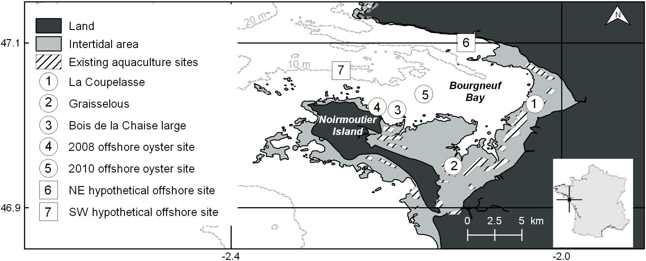
Figure 1. The study site, Bourgneuf Bay, on the French Atlantic coast (indicated in subset). Intertidal (light gray) and offshore (white) zones, in addition to the locations of current aquaculture farms in the intertidal zone and in situ water and experimental oyster sampling sites are indicated.

There are currently 283 mainly small oyster farms occupying leases over approximately 10% of the 100 km² intertidal zone, producing Pacific oysters (Crassostrea gigas) in approximately three-year growth cycles for sale in the local market (Guillotreau et al., 2018). Expanding production to the offshore environment has been of interest to Bourgneuf Bay farmers for some time now, as there is no more room to expand in the intertidal zone. Furthermore, successful offshore experiments in the nearby Marennes-Olérons Bay in the 1990s (Mille et al., 2008) and in Bourgneuf Bay since the late 2000s (Glize and Guissé, 2009; Glize et al., 2010; Louis, 2010) suggest enhanced growth conditions in the offshore environment. Offshore production is seen as a means to increase and diversify production and to shorten the overall production cycle duration within the bay. It is also thought to have the potential to decrease the density of production in the over-crowded intertidal zone, thereby decreasing the probability of disease and related mortality (Pernet et al., 2018).

Satellite Data and Processing

All environmental variables, namely SST, TSM concentration, and Chl-a concentration, were derived from satellite observations. Although more recent satellite data are now available, for example from Sentinel-2 MSI, Sentinel-3 OLCI, and Landsat 8 Operational Land Imager sensors, these are only available for later periods (i.e., from 2015 and 2013 respectively), and as such do not coincide with our earlier in situ data (described in detail below) needed for algorithm validation. MERIS and AVHRR data from 2003 to 2011 were therefore used here. For SST retrieval, the operational non-linear split-window algorithm (Brewin et al., 2017) was applied to data from the US National Oceanic and Atmospheric Administration (NOAA) AVHRR daytime and nighttime scenes with a 1 km spatial resolution. Data from the ESA MERIS have been widely used for the retrieval of optical water quality parameters, including Chl-a as a proxy for phytoplankton concentration and TSM, in a variety of inland and coastal settings (e.g., Matthews, 2011; Odermatt et al., 2012; Blondeau-Patissier et al., 2014; Mouw et al., 2015; Palmer et al., 2015). Nevertheless, there exist no globally-validated retrieval algorithms for the optically dynamic and near-coast environment studied here. Therefore, we investigated full resolution and swath (FRS; spatial resolution 300 m) MERIS data, processed using the Calimnos processing chain, which is designed to dynamically resolve optical water quality parameters in a variety of optically complex inland waters (Simis et al., 2018). Version 1.21 of the processing chain was applied to the 1934 level 1 (L1b) FRS images including our site from the period 2003–2011, and comprised Polymer atmospheric correction with a mineral absorption model, the removal of flagged invalid and suspect pixels, and the application of Chl-a and TSM retrieval algorithms to obtain L2 products.

The MERIS Chl-a and TSM products available through Calimnos and tuned to lake optical properties according to the water types described by Spyrakos et al. (2018) were not found to adequately match the concentrations measured in situ at our site, but several had robust linear relationships with the in situ data. We therefore recalibrated these algorithms for Bourgneuf Bay to improve confidence in the results and applied the recalibrated algorithms to the full time series of interest. The overall best performing algorithms for the detection of water column constituents including both offshore and intertidal matchups (highest coefficient of determination, R², for model fit) were OC2 (O’Reilly et al., 2000) for Chl-a retrieval, which is a fourth-order polynomial relationship between the ratio of the MERIS band centered at 490 nm to that centered at 560 nm and Chl-a, and the Binding et al. (2010) algorithm for TSM, which uses the MERIS band centered at 754 nm in semi-analytical inverse modeling. Recalibration and validation of Chl-a and TSM retrieval algorithms was carried out by splitting our in situ data set into two groups at random; one (70%) to determine the tuning coefficients (i.e., recalibration) and the other (30%) to assess how accurately the tuned algorithm retrieved the absolute concentrations (i.e., validation), in terms of mean bias and absolute and relative root mean square error (RMSE):

$$\text{Bias}=\frac{1}{n}\sum _1^n(M-O)$$

$$\text{RMSE}=\sqrt{\frac{\sum {}_1{}^n(M-O)^2}{n}}$$

$$\mathrm{Rel}.\mathrm{RMSE}(\%)=\text{RMSE}/(\max (O)-\text{min}\left(O\right))\times \mathrm{\hspace{0.33em}100},$$

where M refers to the model-predicted value, O refers to the observed, or in situ-measured value, and n to the number of validation matchups. The original SST retrieval algorithm calibration was similarly validated, but without splitting the matchup dataset into calibration and validation subsets for recalibration.

The archive in situ datasets used to recalibrate and validate the satellite products used in this work comprised measurements made at three locations across the bay; the northern La Coupelasse (47.026 N; -2.032 E) and the southern Graisselous (46.951 N; -2.132 E) sites in the intertidal zone, and Bois de la Chaise large (47.042 N; -2.061 E), located offshore near Noirmoutier island (Figure 1). Multi-parameter water quality probes (YSI 6600) were attached to oyster racks at a height of approximately 0.6 m from the bottom for a duration of two years (2005–2006) at La Coupelasse and Graisselous. These were cleaned manually of biofouling every two months, and turbidity and fluorescence sensors were cleaned with an automatic brush system every 15 min. Hourly measurements of temperature, Chl-a fluorescence, and turbidity, as well as salinity were recorded, and fluorescence and turbidity converted to Chl-a and TSM concentration respectively using field-calibrated relationships obtained and provided in Dutertre et al. (2009). Approximately bi-weekly samples acquired from Bois de la Chaise large for Chl-a quantification by monochromatic spectrophotometry and in situ temperature measurements collected from the surface layer (0–1 m depth) beginning in March 2007 were used here (REPHY, 2017). For all three sites, same-day matchup data were selected from within a 3 h window of the corresponding MERIS overpass, with the closest hour to overpass chosen in the case of the hourly probe data, and comprise the value obtained from the MERIS pixel coinciding with the given in situ sampling location. The total number of matchup points for each parameter and per site, which span all seasons of multiple years, are provided in Table 1.

TABLE 1

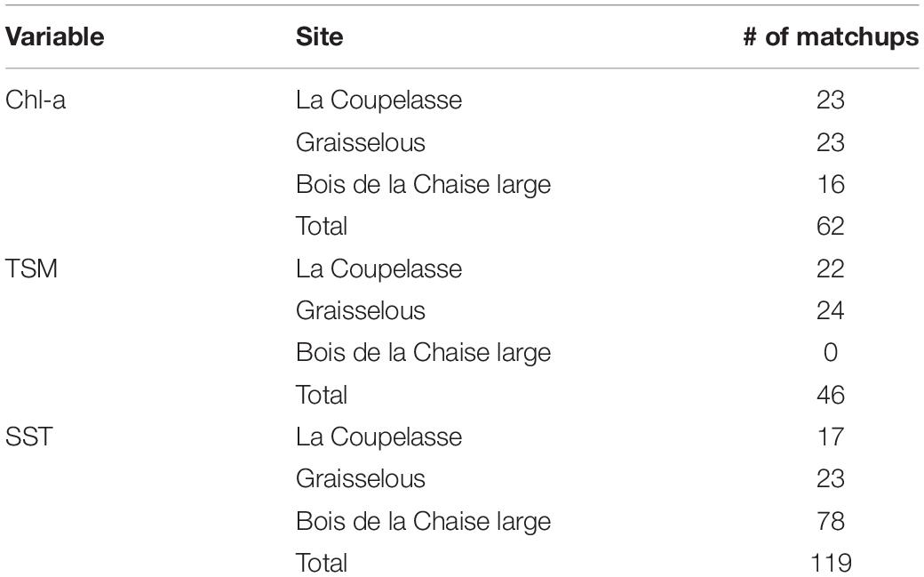
Table 1. Total and per site numbers of in situ-satellite retrieval matchups for each of the variables used as input into DEB modeling.

Following recalibration and validation using daily matchups, all Earth Observation-derived data were processed at and provided by Plymouth Marine Laboratory, and aggregated to L3 ten-day averages from 2003 to 2011 to create the full-year, regular time series data to run the DEB model, given irregular overpass frequency (2–3 days) and gaps from cloud cover in the original data.

Pacific Oyster Dynamic Energy Budget (DEB) Model

DEB theory was used here to model the growth of Pacific oyster. This is a generic (i.e., non-species specific) approach to mechanistically model the uptake and flow of energy through, and eventual growth and reproduction of an organism, based on its environmental conditions (Kooijman, 2010; Sousa et al., 2010). DEB models have been adapted and published for a broad range of species¹.

The DEB model equations and parameters applied here for Pacific oyster are detailed in Thomas et al. (2016), building on previous work by Bernard et al. (2011) and Pouvreau et al. (2006). Essentially, food availability (mainly phytoplankton and resuspended microphytobenthos, represented here using satellite image-derived Chl-a) and water temperature (using satellite image-derived SST in this well-mixed water column) interactively and variably influence rates of ingestion, assimilation, storage, and metabolism, resulting in energy for growth and/or reproduction depending on reserves and additional conditions being met (Figure 2; Thomas et al., 2016). In coastal areas, highly turbid conditions can also have a substantial impact on clearance rate, food consumption, and ingestion (Barillé et al., 1997; Gernez et al., 2014, 2017), subsequently limiting growth. Thomas et al. (2016) have included the effect of high turbidity in Pacific oyster DEB modeling through the inclusion of PIM, which we have also done here (represented using satellite image-derived TSM). The degree to which the ingestion rate is influenced by food availability and TSM in the current work is modeled using calibrated ingestion half-saturation coefficients, X_k and X_ky respectively; all other equations and parameters are those reported in Thomas et al. (2016, S1). Model output is dry flesh mass (DFM; g) and shell length (L; cm) at the same spatial and temporal resolutions as the MERIS input data (i.e., 300 m and every ten days here). To compare with in situ measurements of oyster morphology and to transform into the industry-relevant indicators described below, L was converted to total weight (TW; g) using the biometric relationship found between measurements of the two variables from the extensive Réseau d’observations conchylicoles database (RESCO; Fleury et al., 2018; Equation 1). Flesh weight (FW; g) was likewise calculated from DFM, using the relationship obtained between RESCO measurements from Bourgneuf Bay specifically (n = 2943, R² = 0.83; 2008–2017) (Equation 2).

$$\mathrm{TW}=0.076\times \mathrm{L}{}^3(1)$$

$$\mathrm{FW}=3.99\times \mathrm{DFM}+0.97(2)$$

FIGURE 2

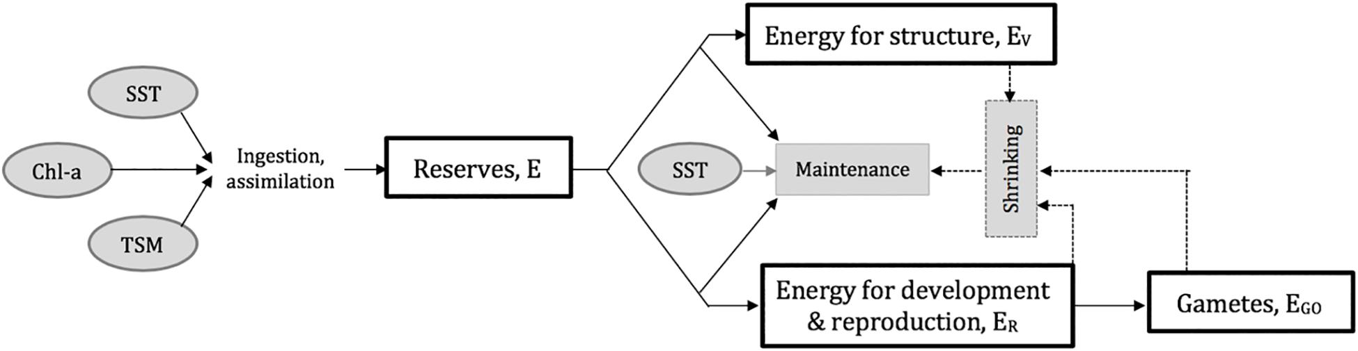
Figure 2. Schematic of the Dynamic Energy Budget (DEB) modified and parameterized from Thomas et al. (2016).

For calibration and validation of the ingestion half saturation coefficients (X_k and X_ky; see above), the DEB model was initialized with oyster measurements made at the beginning of in situ experiments carried out by the Syndicat Mixte pour le Développement de l’Aquaculture et de la Pêche en Pays de la Loire (SMIDAP), a regional association supporting shellfish farmers and fishers, over the course of two growing seasons (2008; 2010) (Glize and Guissé, 2009; Glize et al., 2010; Louis, 2010). The model was run for the specific date range of the in situ measurements for the years in question. The 2010 measurements (May 6 through October 17) were used in the iterative optimization-based calibration, as more data were available and over a longer period for this year. The 2008 measurements and corresponding date range (May 20 through August 14) were then used to independently validate model output with calibration results applied. The model was run for an immersion time of 100% for the offshore site (i.e., constant immersion) and of 75% for the intertidal zone (i.e., under water 75% of the time on average), as calculated by Thomas et al. (2016).

Resulting total oyster weight was extracted for the locations and dates coinciding with the in situ measurements, and model-predicted values were evaluated through regression against measured in situ values. Ingestion half-saturation coefficients were selected in the calibration process as the combination of X_k and X_ky that maximized the coefficient of determination (i.e., R²). Model performance was validated through the mean bias and absolute and relative RMSE. This was carried out for adult and spat life stages separately, given morphological differences between them that may affect ingestion efficiency, and for offshore and intertidal sites, to obtain the ingestion half-saturation coefficients to be used to model the growth of each under various production cycle scenarios.

Pacific Oyster Production Cycle Scenarios and Growth Performance Indicators

Pacific oyster production is typically divided into three stages. The first is pre-growing, whereby spat, often weighing less than 1 g, are grown out to a certain size range (on the order of 10–20 g) for resale, or are then thinned out to allow for sufficient space to continue to grow on the same farm. Here, spat of the industrial size scale T6/T8, corresponding to a total weight of 0.5 g, grown out to size T20/T25, or 14 g total weight, are considered. Although this can take place in marine water or in nurseries, only the former is considered here. From this stage, adults are grown-out to final market size, which ranges from a minimum of 30 g (caliber 5 in France; Table 2) to upward of 150 g (caliber 0 in France; Table 2; Gosling, 2003). Finally, for a short period (several weeks to months) following grow-out, many producers undertake finishing or fattening, which aims to increase the quality index, essentially the fleshiness of the oyster (i.e., ratio of flesh weight to total weight), rather than the total weight, starting with an already market-weight product (i.e., ≥30 g). In France, defined quality index thresholds correspond to certain classes: Normales, Fines, and Spéciales, with Fines obtaining higher market prices than Normales, and Spéciales obtaining higher market prices than Fines (AFNOR, 1985; Gosling, 2003).

TABLE 2

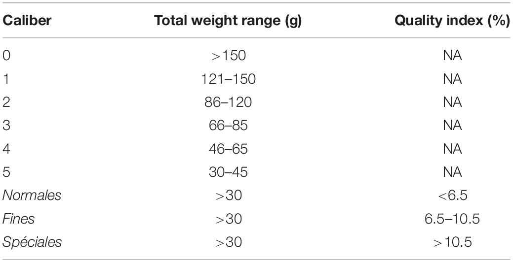
Table 2. Total Pacific oyster weight ranges and quality indices corresponding to French market calibers and classes (AFNOR, 1985; Gosling, 2003).

Validated half-saturation coefficients were used in DEB modeling of the scenarios described in Table 3, and resulting oyster growth curves were transformed into the associated industry-relevant growth performance indicators (Figure 3). In addition to the initial oyster sizes and scenario dates (Table 3), which were chosen in consultation with regional oyster producers and professionals, indicators were also elaborated based on producer and professional input and feedback. These include the time required to reach a target marketable size for both spat (sale to another farm) and adults (sale to market for consumption); total weight achieved by a particular date (here, the main December market corresponding to the traditional peak of oyster consumption for Christmas and New Year celebrations (Buestel et al., 2009), is selected for demonstration); quality index after targeted finishing periods; and the number and timing of spawning events. The latter could be seen as either favorable (i.e., for including or optimizing spat settling and collection as a complementary economic avenue within a grower’s production) or unfavorable (i.e., resulting in additional biofouling as spat settle on cages or other equipment, and (at least temporarily) reducing the quality index of the animal) to production and operations, depending on a particular grower’s specialization and objectives. Overall, our goal was to provide a suite of industry-relevant indicators of which locations would be best suited for oyster farming, and this for various stages and considerations of production.

TABLE 3

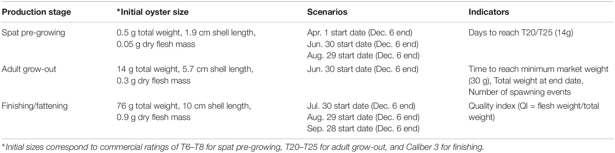
Table 3. Scenarios and indicators for different production cycle stages (spat; adult grow-out; finishing/fattening) processed from Pacific oyster DEB growth modeling.

FIGURE 3

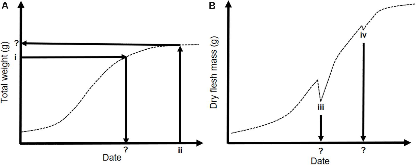
Figure 3. Conceptual schematics of the types of growth performance indicators developed in consultation with oyster growers and professionals and extracted from our modeled growth time series maps. (A) Total oyster weight as a function of time throughout the growing season. (i) Represents the date a target weight is achieved as the parameter of interest, e.g., minimum market weight (30 g). (ii) Takes a given date of interest as the starting point (e.g., early December, in time for the main French oyster market), and looks at what total weight is achieved by this date. (B) Dry flesh mass (DFM) over time throughout the growing season; sharp decreases in DFM indicate spawning events. (iii) and (iv) Indicate the timing of these spawning events, and can also be summed to determine the number of spawning events at a given site in a given year.

Oyster growth curves were generated for each MERIS pixel and for each year of input data (2003–2011). The indicators described above were mapped for each year, and the interannual means and standard deviations were then calculated and mapped, with a single-iteration 3 × 3 pixel median filter applied. By using this multi-year approach, we reduced the chance of unintentionally only mapping an uncharacteristic year (i.e., substantially more or less productive or turbid than usual; much higher or lower temperatures) and thereby capture more typically representative conditions across Bourgneuf Bay. This also allowed us to explicitly consider the interannual variability in the indicators, which is of interest to the farmers, as they seek to optimize production, reducing unnecessary inputs and losses, and therefore seek consistent (akin to more reliable) and stable conditions in addition to higher growth potential.

Demonstration of Offshore and Intertidal Farm Site Comparison

Two hypothetical lease sites were considered; one situated in the northeast and the other in the southwest, near the mouth of the bay (Figure 1). The sites were selected in order to appraise the diversity of growth conditions in the offshore area, the northeastern site being located in more turbid and Chl-a-rich waters than the southeastern site. Each comprised a five-by-five-pixel region of interest, corresponding to approximately 2.25 km² and similar in size to some of the existing leases in the intertidal zone (Figure 1). Descriptive statistics were then extracted and visualized for each hypothetical offshore farm and for the existing intertidal leases for comparison, for each selected growth indicator. Following testing for normality (Shapiro–Wilk) and equal variance, the annual means of each indicator were also compared between sites through parametric one-way ANOVA, or using the Kruskall–Wallis one-way ANOVA by ranks when either normality (Shapiro–Wilk) or equal variance testing failed, with post hoc Tukey tests for pairwise comparison. In all cases, an α = 0.05 was selected for significance.

Results

Satellite Input Data Calibration, Validation, and Mapping

Results from the empirical recalibration and validation of Chl-a (OC2) and TSM (Binding et al., 2010) retrieval algorithms, and the validation of the original SST (operational NOAA AVHRR) calibration, can be found in Figure 4. For Chl-a and TSM, retrievals using the original algorithm parameterization showed either a strong linear over- or underestimation (Figures 4A,C), and linear recalibration (n = 44 and 32 respectively) was therefore performed (Figures 4B,D), improving retrievals of the three parameters, with only slight positive mean bias in the satellite retrievals for each (Chl-a = 0.74 mg m^–3, n = 18; TSM = 2.6 g m^–3, n = 14). The original SST calibration (n = 119) was found to sufficiently reproduce in situ measurements from the three sites (Figure 4E), and was therefore applied as-is to the nine-year time series.

FIGURE 4

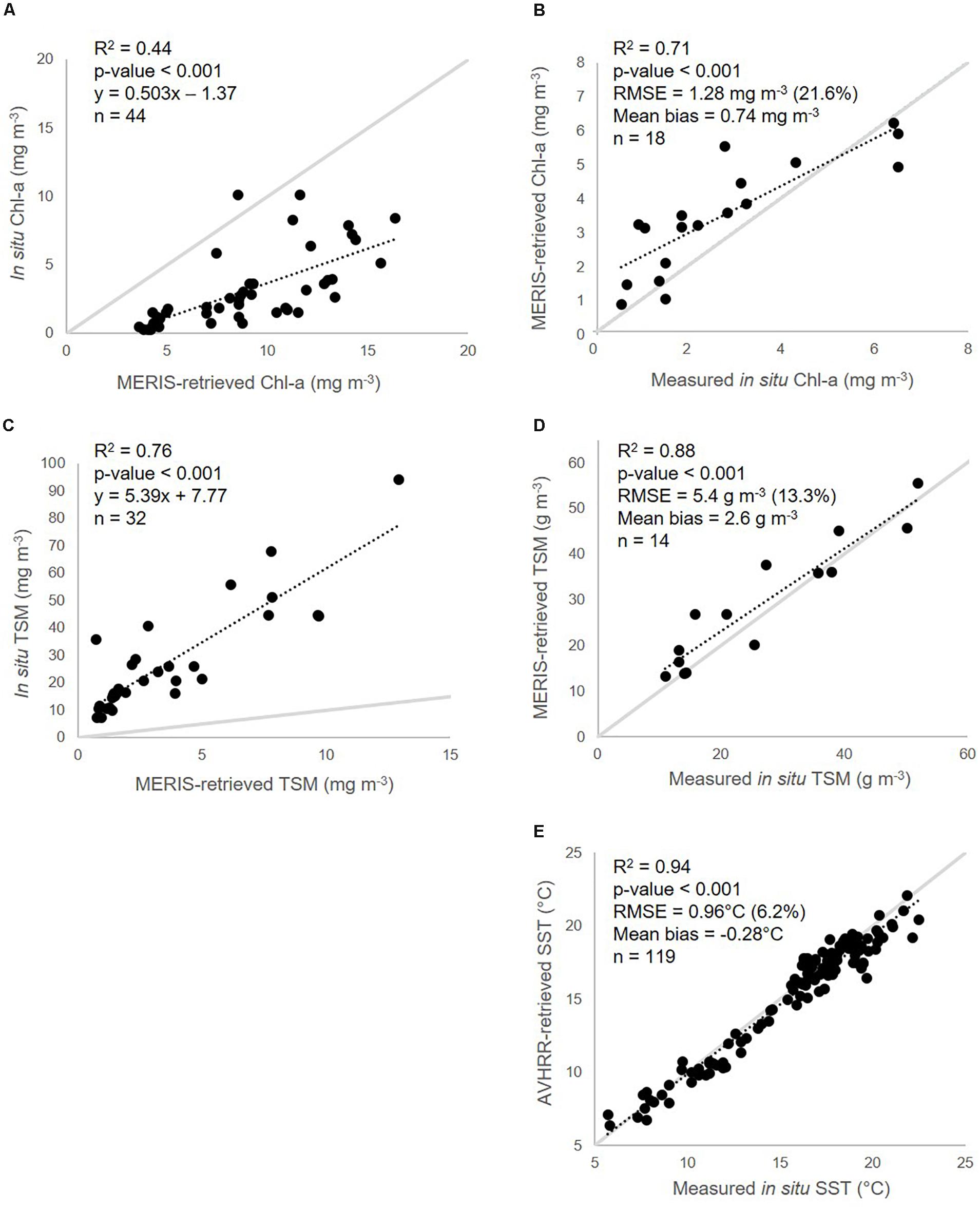
Figure 4. Recalibration (A,C) and validation (B,D) of MERIS OC2 Chl-a (A,B) and Binding et al. (2010) TSM (C,D) retrieval algorithms, and validation of original SST (E) retrieval algorithm calibration, used to drive the DEB model, with corresponding in situ data from Bourgneuf Bay (Figure 1).

Maps of the interannual mean and standard deviation of the three parameters (Figure 5) highlight the general spatial patterns observed and their interannual variability across Bourgneuf Bay. As expected, both Chl-a (Figures 5a,b) and TSM (Figures 5c,d) are higher on average and more variable in the intertidal and adjacent areas than further offshore at greater water depths, with both the absolute concentration range and variability of the latter being much greater. Likewise, higher average SST (Figure 5e) is found in the nearshore areas, with higher variability in the central bay (Figure 5f).

FIGURE 5

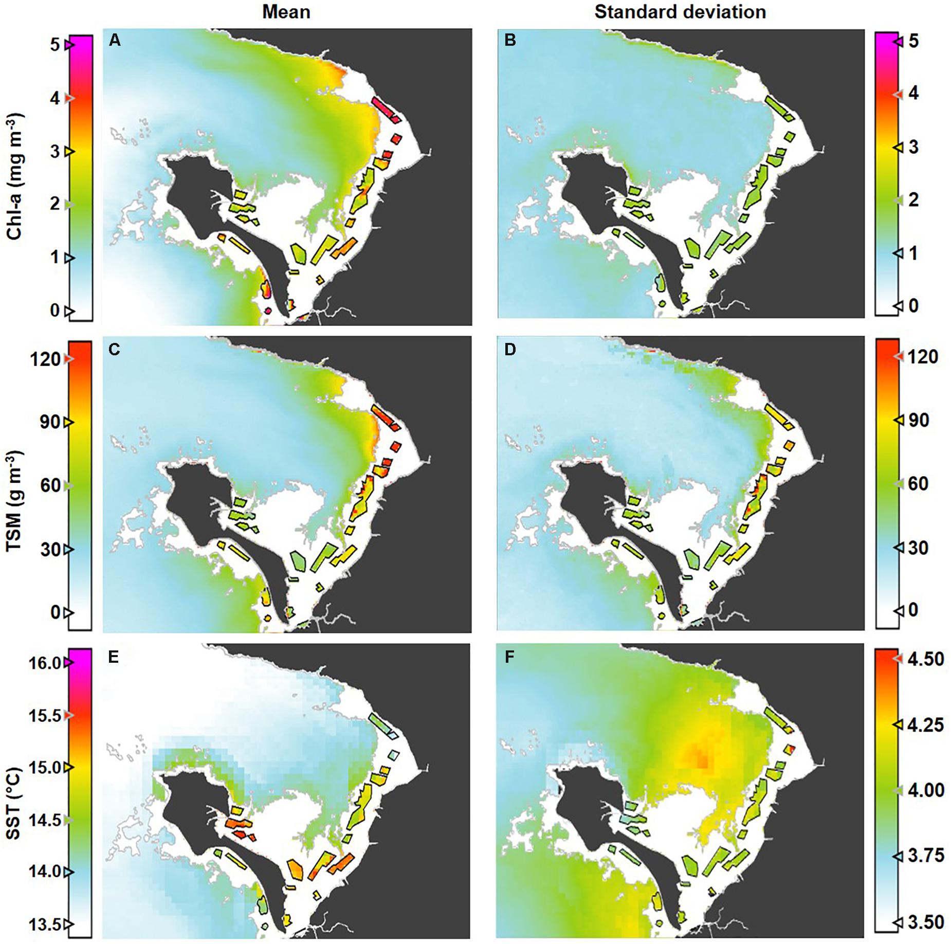
Figure 5. Maps of interannual mean (left) and standard deviation (right) for input products across the full nine-year time series; (A,B) Chl-a, (C,D) TSM, and (E,F) SST. In the intertidal zone, the Chl-a, TSM, and SST mean and standard deviation are shown within the farming sites only (i.e., unmapped for the white area).

DEB Model Calibration and Validation

A good fit was found between DEB-modeled spat and adult oyster total weight growth and weights measured in situ throughout the growing season following calibration of the ingestion half saturation coefficients, X_k and X_ky (Figure 6 and Table 4). Modeled spat (0.5–13.45 g) and adult (20.9–47.1 g) total weight corresponded to a RMSE of 1.30 g (13.4%) and 4.34 g (17.4%) and mean biases of 0.55 and -3.37 g respectively, compared with measured in situ values. In both in situ measurements and modeled values (in both 2010 and 2008), we see higher weight gain offshore compared with the same amount of time in the intertidal zone. This is most notable for 2010, for which in situ measurements were taken over a longer period than in 2008 (May 1 through October 17 versus May 20 through August 14), thereby allowing growth to heavier weights to be achieved. Even spat grown from an initial weight of < 1 g were able to reach market weight offshore by mid-September (Figure 6A) in 2010, although this was slightly underestimated by the MERIS-DEB-modeled results. Note that initial measurements (i.e., from May 1, 2010 and May 20, 2008) were used in model initialization for calibration and validation respectively, and therefore were not included in matchup statistics or graphing.

FIGURE 6

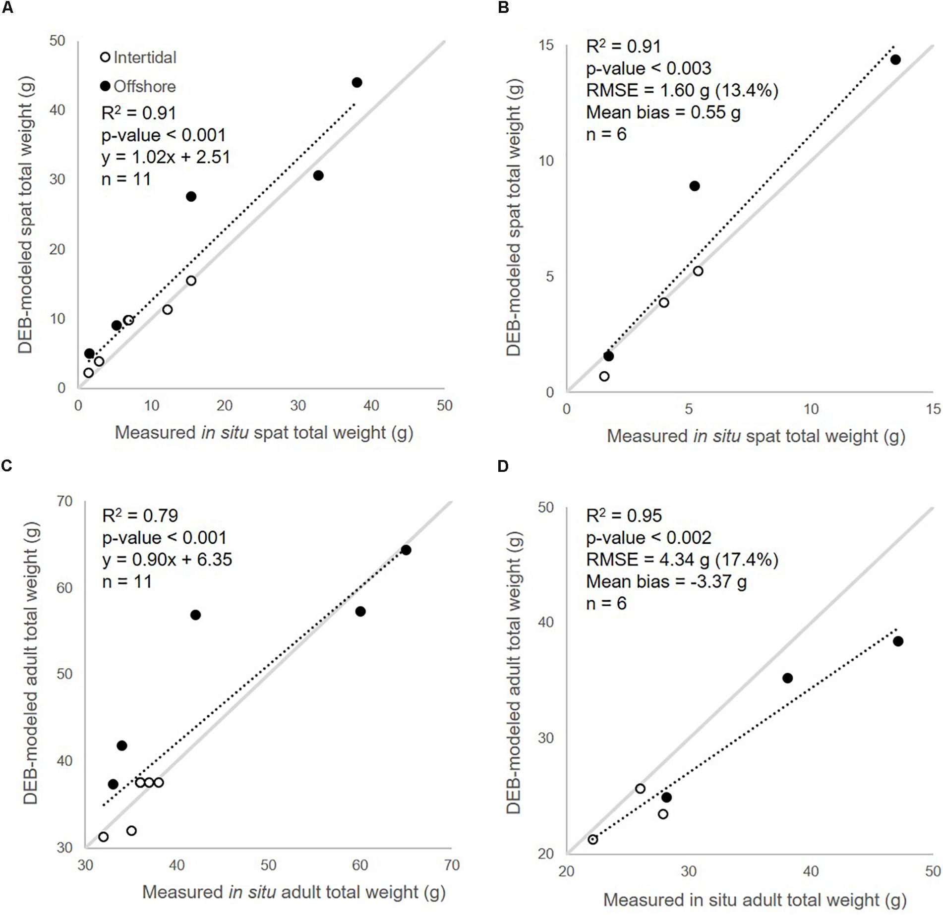
Figure 6. Calibration of DEB-modeled (A) spat and (C) adult growth using corresponding 2010 in situ data from intertidal and offshore zones; validation for spat (B) and adult (D) growth modeled with calibrated coefficients using in situ data from 2008 (see Figure 1 for sampling locations).

TABLE 4

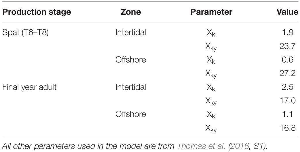
Table 4. Calibrated half-saturation coefficients (X_k, X_ky) used in MERIS-driven DEB modeling of Pacific oyster spat and adult growth, and applied to all nine modeled years.

Growth Indicator Mapping

The Pacific oyster production scenarios and growth indicators detailed in Table 3 were modeled for each of the nine full years of satellite image input data. For each scenario, the resulting interannual mean and standard deviation are mapped in Figures 7, 8 respectively. Mapping trends across the nine indicators and three production cycles suggest generally enhanced growth in the northeastern offshore segment of the bay across all indicators, higher than in the intertidal zone where production is currently practiced and higher than in the southwestern offshore segment (Figure 7).

FIGURE 7

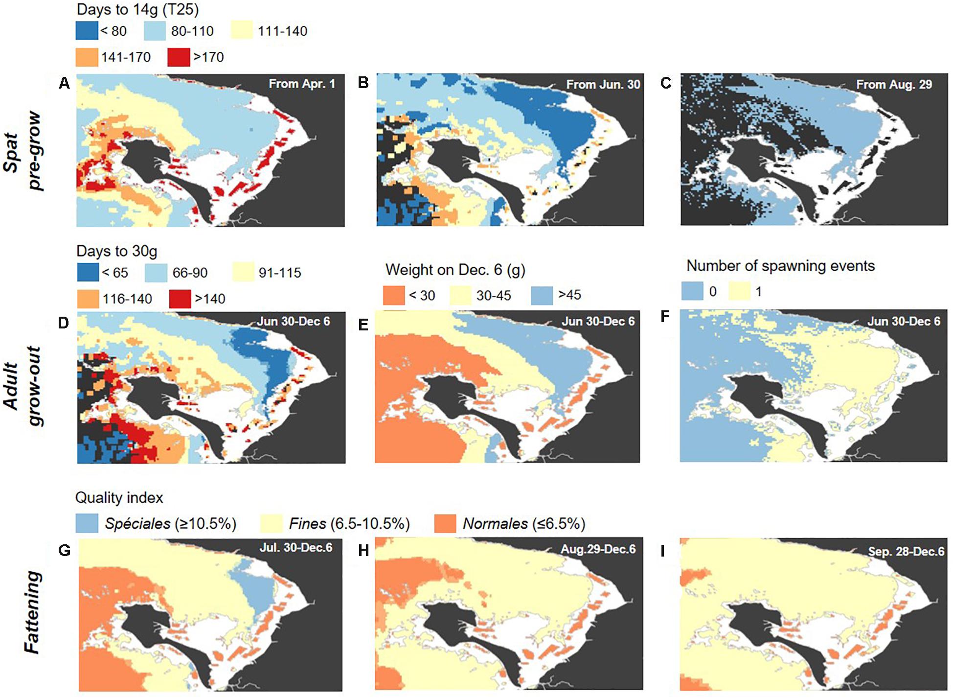
Figure 7. Maps of the nine-year interannual means for the scenarios and growth indicators detailed in Table 3, for the spat pre-growing phase (A–C), from an initial T6–T8 (0.5 g) size, adult grow-out phase (D–F), from an initial T25 (14 g) size, and final fattening phase (G–I), from an initial Caliber 3 Normale size (76 g; QI = 6%). Note that dark gray water areas in a-d correspond to areas where the target weight (i.e., 14 g for spat and 30 g for adults) was not achieved by the end of the growing season.

FIGURE 8

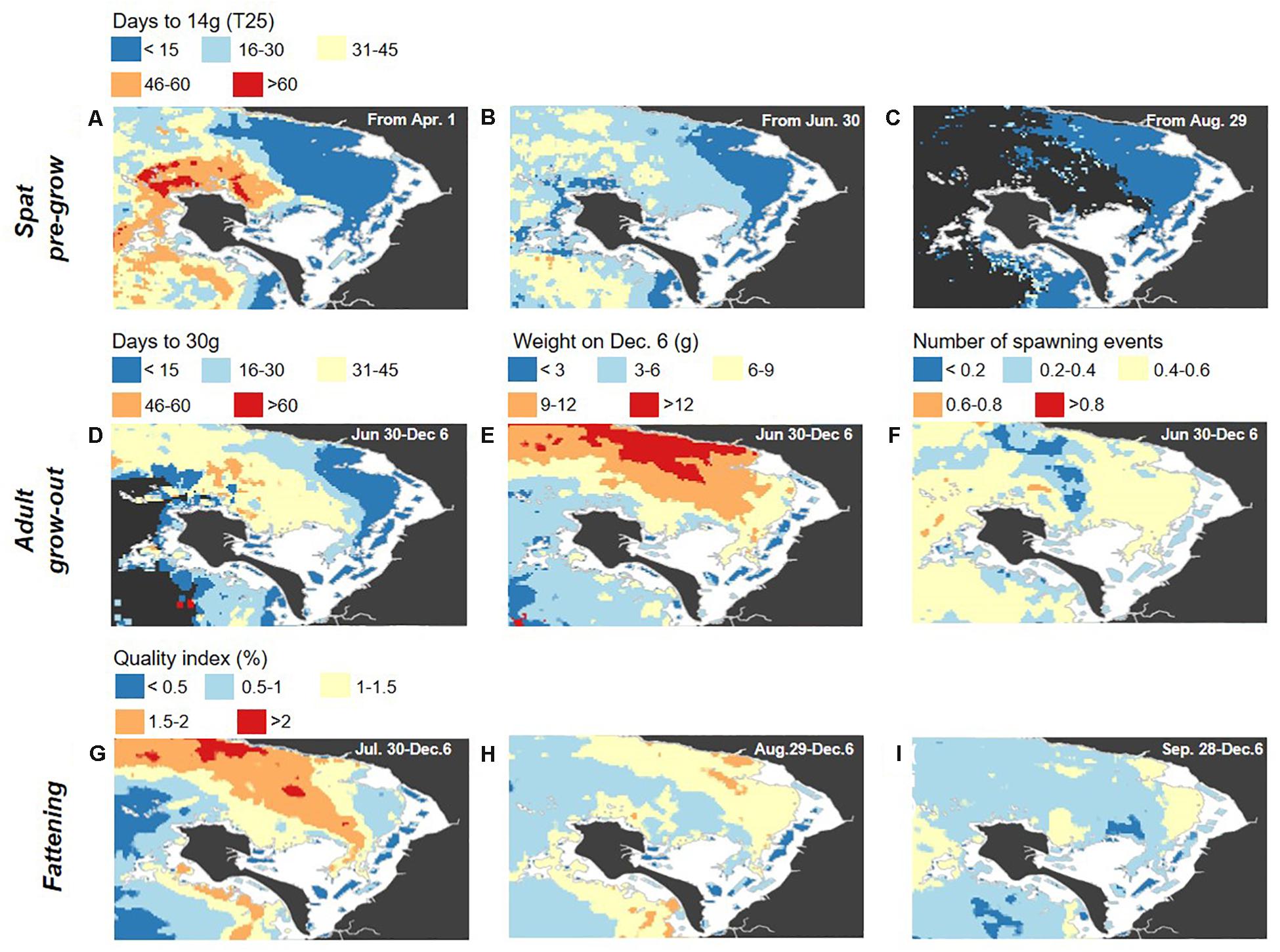
Figure 8. Maps of the nine-year interannual standard deviations for the scenarios and growth indicators detailed in Table 3, for the spat pre-growing phase (A–C), from an initial T6–T8 (0.5 g) size, adult grow-out phase (D–F), from an initial T25 (14 g) size, and final fattening phase (G–I), from an initial Caliber 3 Normale size (76 g; QI = 6%). These correspond to the means presented in Figure 7. Note that dark gray water areas in (A–D) correspond to areas where the target weight (i.e., 14 g for spat and 30 g for adults) was not achieved by the end of the growing season.

For the spat pre-growing phase, industry size T6–T8 spat (initial total weight of 0.5 g) were put in place at staggered start times (April 1, June 30, and August 29) and highlight that, in the northeastern offshore segment of the bay, it would be possible to begin this phase at later dates than in the southwestern offshore and intertidal areas, as late as the end of August (Figure 7C), and still achieve the target size (T20–T25; 14 g) for sale in under 2 months. Indeed, in the intertidal area, pre-growing must begin in the spring to achieve the target weight gain of a T20–T25 spat by October, over 6 months later. In the southwestern offshore segment, it must begin by early summer at the latest (i.e., June 30; Figure 7B), to reach the target weight within 6 months, by late November/early December.

For adult grow-out, a single time frame was considered (June 30 through December 6), but three different growth indicators were of interest. First, the time to reach the minimum market size for consumption (30 g; Figure 7D) as well as the total weight by early December (Figure 7E) were jointly assessed as they are of primary interest for the industry. Although minimum market weight was able to be reached for a few, dispersed areas in the intertidal zone for an average year, this took until the end of the growing season considered here (i.e., early December, after 160 days), which was also the case for the southwestern offshore segment (Figure 7D). Instead, 30 g (i.e., minimum market weight) is achieved by mid-August to early October on average on the northeastern offshore segment (Figure 7D). Total weight by early December, for the initial conditions and dates considered here, tends to remain on the order of 15–25 g (Figure 7E) for the southwestern offshore area and the existing intertidal farms, and oysters would require another season before marketable. In contrast, total weight by the end of the season for the northwestern offshore segment is on average greater than 45 g for some areas (i.e., Caliber 4 oysters; Table 2 and Figure 7E). Certain offshore areas, notably the eastern and central portion of the bay, are associated with slightly more spawning activity on average (Figure 7F), which could indicate areas to avoid or to target for farm placement, depending on whether spat collection is foreseen as part of a given production cycle.

The quality index and classification according to French standards (Normales, Fines, or Spéciales) for sale to the main French market in early December that was achieved by starting at three different dates, from large Caliber 3 (76 g) Normales oysters (QI = 6%) was considered for a final fattening phase (Figures 7G–I). Throughout most of the intertidal area, only Normales classification was achieved on average (orange in Figures 7G–I), whereas at least Fines was possible throughout much of the offshore area (pale yellow in Figures 7G–I). An early start to fattening (late July/early August) resulted in Spéciales classification over a large part of the offshore area (blue in Figure 7G).

Intertidal and Offshore Farm Site Comparison

Modeled growth indicators were compared statistically for the two potential offshore farm sites located in contrasting conditions, one in the northeastern segment of the bay, the other in the southwestern segment, with average values across existing farms in the intertidal zone (Figure 9). Although these hypothetical sites were chosen here to simplify the demonstration of our approach, such a comparison could be made for any selected site, and these findings are expected to extend beyond the hypothetical new farm sites considered here, with similar findings mapped across larger areas in Figures 7, 8.

FIGURE 9

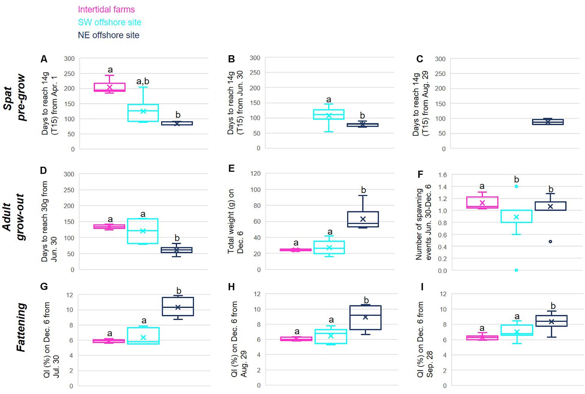
Figure 9. Comparison of interannual indicator values for two hypothetical offshore sites (see Figure 1) (dark blue (NE) and turquoise (SW)) and existing intertidal farms (pink) for the scenarios and growth indicators detailed in Table 3, for the spat pre-growing phase (A–C), from an initial T6–T8 (0.5 g) size, adult grow-out phase (D–F), from an initial T25 (14 g) size, and final fattening phase (G–I), from an initial Calibre 3 Normale size (76 g; QI = 6%). Different letters above boxes are associated with statistically different groups (Kruskall–Wallis one-way ANOVA on ranks and Tukey test p < 0.05). Note that missing boxes associated with given sites (B,C) correspond to the target weight not being achieved for that site within the defined time range.

It is clear that although enhanced growth is expected in the offshore environment, as already observed in in situ experimental data for single point locations (Figure 6) and in mapped interannual average indicator values (Figure 7), this is highly variable across the approximately 240 km² of the offshore area considered. Notably, we consistently see faster growth and higher quality products at the northeastern site (Figure 9; dark blue box), with the southwestern site (Figure 9; turquoise box) most often either statistically indistinguishable (KW and Tukey test p < 0.005) from growth on the existing intertidal farms (Figure 9; magenta), or falling in between the NE and intertidal sites. Exceptions are the number of days for spat to reach 14 g from the second start date, June 30, where this is reached for the SW site, but not in the intertidal zone (Figure 9B), and the slightly higher average number of spawning events per year observed in the intertidal zone, with the two offshore sites statistically indifferent (Figure 9F).

Discussion

DEB Input and Output Validation: General Findings and Limitations

Due to the empirical calibration of Chl-a and TSM algorithms, these are only considered to be valid for Bourgneuf Bay without wider validation, and specifically for the conditions encountered in the in situ matchup dataset. This remains an important consideration here, and in the use of calibrated satellite products for water quality parameter retrieval generally. Ongoing work on automatized algorithm selection based on satellite-observed optical characteristics promises a robust solution to this issue through the provision of more globally-valid products (e.g., work of Spyrakos et al., 2018; Neil et al., 2019 for lakes), but was not yet adapted for the optical conditions of our site for use in this work. Similar validation, and possibly calibration, of satellite products would also be required in future work at other sites until a more automated approach is available, and limits the spatial range over which results can be expected to be valid. Given the range of conditions and temporal coverage (i.e., interseasonal and interannual; spanning all seasons of several years, as well as multiple sites within the bay comprised of contrasting conditions) of the in situ matchup dataset, such local calibration was possible in the current work and the resulting satellite products are expected to adequately represent the conditions for the area and time period of interest for the current modeling application.

For both DEB modeling results and input parameter validation, single-point measurements taken in situ are compared with satellite pixel data integrating the signal of 0.09 km², which is a well-known source of error inherent to the methodology. In addition, whereas same-day matchups were used to calibrate and validate the input products, in the DEB modeling, daily images were aggregated to ten-day mean products to reduce gaps and noise in the data. Modeled oyster growth extracted for matchup validation are then the ten-day modeled periods within which the given in situ measurements were taken, and represent an additional, temporal source of uncertainty. More recent satellite image data, for example from the ESA Sentinel-2 MultiSpectral Instrument and Sentinel-3 Ocean and Land Color Imager, improve upon the spatial and temporal resolutions respectively of the data used here and the availability and use of such higher resolution data will offer potential new insights and directions for future work. It is also worth noting that although the oyster growing season typically begins in March and ends in December, in situ data were only available from May through August (2008) and October (2010), which corresponds to the period of most and most rapid growth in the year. Nonetheless, growth dynamics were found to be well-captured here using the coupled MERIS-DEB results. Following the calibration of the half-saturation coefficients (X_k, X_ky), modeled results were found to robustly capture oyster growth over time, for spat as well as for adults, and for both intertidal and offshore sites alike. The differences in the half-saturation coefficients resulting for the two life stages may be explained by developmental differences in their gills and labial palp morphologies affecting their respective ingestion efficiencies (Dutertre et al., 2007, 2017). With regard to site differences, food quality (and phytoplankton composition in particular) is recognized to be key to bivalve nutrition (Picoche et al., 2014). Differences in the composition of phytoplankton communities between the intertidal and offshore sectors could therefore explain the differences in X_k, which were higher in the intertidal sector for both spat and adult oysters. The high Chl-a concentrations measured in the intertidal zone may therefore be associated with phytoplankton or resuspended microphytobenthos of poorer food quality, in addition to the negative impact of the higher turbidity on oysters’ filtering ability.

Given the investigative and experimental nature of offshore oyster cultivation in this area, in situ data for model calibration and validation are limited to only the two periods presented here (2008 and 2010), each with only one intertidal and one offshore site. These are, however, expected to represent the main component of variability in the input parameters, and therefore in oyster growth, within the bay overall. As for the satellite input data, however, empirical DEB model calibration using this local in situ data means that application of this model and similar methods at other sites would require recalibration with data from the given site. As offshore shellfish production remains quite experimental in nature and is not common either commercially or experimentally, such data are very seldom available and may present a barrier to carrying out similar future work elsewhere. Monaco et al. (2019) observed the inability to transfer DEB parameterization of the Mediterranean mussel (Mytilus galloprovincialis) validated at a native site to a South African site and suggested unaccounted environmental variables and phenotypic plasticity as underlying this observation. Proposed alternatives to address the issue related to the former explanation are by adapting the ingestion half-saturation coefficients as a function of the given phytoplankton density (Alunno-Bruscia et al., 2011) or the ratio of Chl-a to TSM (Thomas and Bacher, 2018), providing a means to apply such work across larger spatial scales without needing to manually recalibrate the half-saturation coefficients.

Spatial Trends in Growth Parameters to Inform Site Selection

In all of the mapped oyster growth indicators (Figure 7) and their interannual variability (Figure 8), variability across the bay is clearly observed, including between farmed intertidal sites and the offshore environment, as well as across the offshore environment itself. Although oyster growth clearly has high potential offshore, improving greatly upon the intertidal status quo in some areas, this is not spatially uniform. Instead, this is highly variable, and there are large areas of the offshore environment where production is expected to not be even as good as in the intertidal area where farming currently takes place, in addition to the areas where higher growth would be expected. Generally, there is a consistent spatial gradient, with greater growth potential in the northeast offshore segment of the bay and less in the southwest offshore segment, found to be comparable or sometimes even less favorable than in the intertidal zone. This highlights the value of using spatialized data in such an approach, as the finding from in situ data alone that growth is higher offshore is limited spatially and may be misleading when proceeding to either future experimental work or commercial operations offshore, depending on where in the bay they are located. For example, locating a new cage or farm where the 2010 experimental cage was located (Figure 1) would not result in the most optimal growth possible within the bay, and locating it further west (e.g., just north of Noirmoutier island) would result in even more limited growth (Figure 7). The results from the current work then guide more optimal offshore cage or long-line placement as a result of their spatially-explicit nature.

The overall spatial structure in the resulting mapped indicators is, expectedly, due to the variability observed in satellite image input parameters, Chl-a, TSM, and SST, which underlie oyster growth. The very high TSM concentrations in the intertidal zone are at levels that substantially limit oyster growth in this area (Gernez et al., 2014). TSM concentrations gradually become lower and reach sub-impacting levels offshore, but Chl-a also decreases toward the offshore environment in a similar fashion. The spatial patterns in both TSM and Chl-a are expected to be related to benthic resuspension only possible at shallower depths, with water column Chl-a concentrations comprising phytoplankton and resuspended microphytobenthos (Hernández Fariñas et al., 2017), as well as current and water circulation patterns. Concentrations of both in the offshore waters are higher in the northeastern segment of the bay, but the yearly average TSM seems to be low enough to not hinder growth. In the southwestern segment, however, where TSM concentrations are lower, Chl-a concentration is also too low to support accelerated growth compared with the intertidal zone. At the temperatures observed for Bourgneuf Bay, higher SST is generally expected to promote oyster growth, and there is a more linear gradient from near- to offshore compared with Chl-a or TSM, with overall warmer temperatures in shallower waters. Multiple spawning events (Figure 7F) are also associated with these generally warmer shallower areas (Figure 5E) and with areas with higher SST variability (Figure 5F), likely due to the required 18°C spawning threshold being met or exceeded more frequently (Barillé et al., 2011). Additionally, outside of the intertidal zone, oysters are immersed in the water full-time (i.e., 100% immersion), whereas the average immersion time for intertidal zone farms is only 75% (Thomas et al., 2016, Suppl. Info). This means that on average oysters are able to ingest food 25% less of the time in the intertidal zone compared with offshore. In preliminary sensitivity analyses carried out ahead of this work, the variability of immersion time was also found to significantly affect resulting oyster growth, and to play a role in the higher growth observed offshore.

For spat, the consistently faster growth observed in the northeastern offshore segment over the different timeframes tested suggests that pre-growing multiple batches of spat within the same year may be possible there. For example, starting pre-growing in early April, as in Figure 7A, the target 14 g is achieved within approximately 90 days, corresponding to late June, potentially allowing for a second or even third pre-growth cycle for those farmers choosing to specialize in spat production for resale or to stock other concessions within their own production. Likewise, the later start of a single offshore pre-growth cycle may be chosen to better fit within a farmer’s overall production, which may include other phases, or to better coincide with sale or thinning (i.e., when oyster densities are reduced to allow continued growth on the same farm) dates of interest. Comparatively, to achieve the target spat weight (14 g) over the full time period (eight months) considered here, spat cultivation would need to begin in the spring in the intertidal zone, or early summer at the latest in the southwestern offshore segment (Figures 7A–C), and only one cycle per year would be possible.

Alternatively, rapid adult oyster growth offshore (Figures 7D,E) may allow producers to purchase pre-grown spat, specialize in the offshore adult production stage, and either move adults to a fattening pond within their own operation or sell to a fattening-specialized grower, keeping this part of their production cycle to within a single year. Overall, in moving either adult or spat production offshore, approximately a full year of the total production cycle can be saved, reducing this from approximately three to two years. Producers may also consider areas with higher spawning potential (in the central-eastern and intertidal areas of the bay; Figure 7F) as either favorable, in cases where spat capture is targeted as part of their overall production and therefore desirable, or unfavorable, where capture is not intended and rather leads to issues of biofouling, requiring added maintenance, and decreased quality index, at least temporarily.

Fattening may also be possible offshore, in the northeastern segment of Bourgneuf Bay (Figures 7G–I), allowing Fines, if not Spéciales, classification, and removing the need for a separate fattening facility (ponds, typically located inshore and with high concentrations of phytoplankton). Although interannual variability was found to be slightly higher at the northeastern offshore hypothetical site considered here than elsewhere in the bay (Figures 8, 9G–I), it is still relatively low, such that at least Fines and possibly Spéciales class oysters could be expected from year to year, compared with consistently Normales in the intertidal zone. However, attaining the higher Spéciales classification was found to only be possible by beginning fattening in the summer months, suggesting that flesh weight gain during the late summer/early fall months can be critical in natural waters under the scenarios considered. All options are to be considered by producers in terms of the cost-benefit balance of moving offshore for their given situation, for any production stage of interest, and with particular consideration for risks, infrastructure and technical investment, and additional (or less) labor that would be required of them (Buck and Langan, 2017).

Adaptability of Growth Indicators and Production Scenarios

Given the nature of the DEB model outputs driven by remote sensing data, mapped and at regular time steps, oyster growth can be transformed to provide meaningful information to producers or other decision-makers or professionals, and targeted to their specific cases and interests. A suite of indicators was selected here to demonstrate the broad range of indicator types possible to easily adapt to a particular production specialization of interest. For example, Bourgneuf Bay oysters are sold for consumption primarily within the local market, with peak sales and therefore target peak production, occurring in December, in association with the French tradition of eating oysters at Christmas and New Year celebrations (Buestel et al., 2009). An additional summer market was indicated as being of secondary interest in France, and may be the primary domestic market in other oyster-producing countries. Although not demonstrated here, a similar exercise could be undertaken targeting, for example, starting production in spring and assessing adult oyster weight achieved in July, or another date deemed to be of interest for a particular site. Likewise, whereas minimum weight for the French market (30 g) was considered here, a range of different production targets could be considered, in terms of product size and weight, notably considering the different market calibers (Table 2), where the most popular size is typically considered to be Caliber 3 (ranging from 66 to 85 g total weight). Several examples, for spat, adult, and finishing stages have been demonstrated in a mapping and statistical application here, but weight thresholds and timings can easily be adjusted to correspond to specific calibers or other targets.

Likewise, various scenario combinations could be considered, including different start dates and moving oysters between offshore and intertidal concessions at different stages. The start and end dates considered are part of model initialization and can be modified to correspond to a particular scenario of interest. Faster growth is observed for both spat and adults in the northeastern offshore segment compared with the intertidal zone, and other noted benefits include reduced mortality from viral disease (Pernet et al., 2018). However, it is generally considered unfavorable to complete an entire production cycle (i.e., spat through market size) offshore. This is due to observed physiological effects (e.g., underdeveloped adductor muscles; relatively weak or malformed shell) and parasite damage, such as from the shell-boring worm, Polydora sp. (e.g., Glize et al., 2010), associated with constant immersion, and the negative impact on the marketability of the resulting product. Given the various possible offshore and intertidal production cycle stage combinations (e.g., beginning with pre-growing in the intertidal zone, then moving offshore for grow-out or finishing or vice versa), and this imperative to choose which production cycle stage would best be moved offshore, potential time savings and other gains generated by completing different stages within the full production cycle offshore versus in the intertidal zone can be assessed and compared. Again, the farmer can then determine if such gains are worth the various investments that would be required in moving part of their production offshore and optimize which phases take place where (i.e., offshore or in the intertidal zone).

Additional Considerations for Site Selection and Future Directions

An important consideration that is beyond the scope of the current work is the effect of stocking density and carrying capacity on growth potential (Smaal and Van Duren, 2019). Trophic interactions and population dynamics are not considered here, and carrying capacity is known to be a limitation to production within the bay (Le Grel and Le Bihan, 2009). Indeed, the current modeling is based on a calibration where quite dense oyster cultivation takes place in the intertidal zone, where more than 5,000 tons of Pacific oyster are harvested per year (Agreste, 2015), but no cultivation takes place offshore (i.e., the current results relate to a single cage with no additional cultivation in the vicinity, as per the experimental data used for DEB calibration and validation). This can be expected to have an impact on modeled results, favorably biasing offshore growth potential. Were stocking density to increase offshore, through adding concessions there, growth potential could reasonably be expected to decline as carrying capacity is met or especially if it is exceeded. Furthermore, the addition of more farms to the bay could be expected to impact the overall carrying capacity at the bay level, and adding farms offshore may also negatively affect existing cultivation in the intertidal zone. Offshore leases could be offset by requiring that an equivalent lease be ceded in the intertidal zone (Le Bihan and Le Grel, 2008). As a next step, the inclusion of carrying capacity assessments (e.g., Filgueira et al., 2015) to inform farm and stocking density would be invaluable. Likewise, the environmental impacts of shellfish farms, via their enrichment of surface sediment organic matter, have been modeled using spatialized data elsewhere (Brigolin et al., 2017), and should be considered in offshore site selection for Bourgneuf Bay in terms of overall sustainability.

The value of using remote sensing data has been demonstrated here for modeling growth potential, and its use could be extended to coupling with other models to inform shellfish aquaculture [e.g., scope for growth (e.g., Barillé et al., 2011), the R package for AquaCulture (RAC; Baldan et al., 2018), ShellSim (Ferreira et al., 2008; Hawkins et al., 2013), Farm Aquaculture Resource Model models (FARM; Ferreira et al., 2007)]. DEB modeling, like several of these alternative or complementary models, is generic, simulates the entire life cycle of species, and elsewhere has been parameterized for a variety of species, including several of interest from an aquaculture perspective and in Bourgneuf Bay in particular. These include blue mussel (Thomas et al., 2011) and great scallop (Gourault et al., 2019). Given in situ data for the location and species of interest, other potential opportunities for farmers could be similarly assessed and compared, and included in broader feasibility and economic analyses.

Whereas the use of satellite remote sensing only allows the retrospective consideration of conditions at potential or current aquaculture sites, coastal zones and shellfish are known to be sensitive to the effects of climate change (Thomas et al., 2016, 2018; FAO, 2018). A similar approach as presented here could also make use of spatialized data from ecological models, such as the Finite Volume Coastal Ocean Model (FVCOM; Cowles, 2008) or the Proudman Oceanographic Laboratory Coastal Ocean Modeling System (POLCOMS; Holt and James, 2001) coupled with the European Regional Seas Ecosystem Model ERSEM (Baretta et al., 1995; Butenschön et al., 2016), to consider present-day as well as various future climate change scenarios to more fully plan for these potential effects in choosing and developing new aquaculture sites (e.g., Palmer et al., 2019). Such data often provide fuller spatial and temporal coverage than satellite observations, since issues like cloud cover do not apply. Like satellite data, such data are associated with their own inherent error and uncertainty and with trade-offs in terms of their spatial resolutions and coverage (i.e., POLCOMS-ERSEM spans all of the western North Atlantic and Mediterranean, but at a 0.1° spatial resolution; Ciavatta et al., 2016).

In addition to the growth potential, assessed here, which is crucial and underlies the potential success of a given operation at a given location, such results should eventually be combined with other environmental, technical, and socioeconomic considerations (Longdill et al., 2008; Brigolin et al., 2017). Barillé et al. (forthcoming) have assessed a suite of these for offshore Pacific oyster cultivation at the regional scale within which Bourgneuf Bay is located, and note in particular that bathymetry, as well as distance to and harbor capacity entail real constraints to which locations the small-scale producers of Bourgneuf could consider in terms of what upgrades to materials, boats, and then boat licenses would be required should certain ranges be exceeded (i.e., bathymetry ranging from 5 to 10 m for cages and from 10 to 20 m for longlines, and within 5 nm of a harbor with sufficient capacity). Certain other environmental and socioeconomic factors were likewise found to impose constraints as to where aquaculture would be feasible (e.g., areas where protected habitat or fishing areas are found, of seabed mining, sand deposits, or commercial traffic channels). Others were considered in terms of their favorable or unfavorable impact, but were not considered preclusive to oyster cultivation (i.e., presence of underwater pipes or cables, militarized zones, current rates and benthic substrate type) in resulting suitability indices. Whereas physical conditions (e.g., wave height, swell) will substantially limit which sites are suitable in more exposed open ocean sites (Buck and Langan, 2017), for the relatively sheltered conditions within Bourgneuf Bay, even offshore, this is not expected to be a major issue. Barillé et al. (forthcoming) also considered DEB-modeled oyster growth, but using reduced resolution input products more relevant to the regional-scale analysis they undertook, and therefore at a much coarser scale than is demonstrated here. The combination of a GIS-based spatial multi-criteria evaluation with the oyster growth indicator mapping at a finer spatial scale relevant to site selection at the bay scale, as demonstrated here, will be invaluable next step in moving Pacific oyster production offshore in Bourgneuf Bay.

Conclusion

Here, medium-resolution satellite data were coupled with ecophysiological DEB modeling to demonstrate the feasibility, but also the high degree of spatial variability of offshore Pacific oyster growth potential in Bourgneuf Bay, France, where cultivation currently takes place in the intertidal zone with little to no room for further expansion. Both satellite (MERIS and AVHRR)-derived input products, Chl-a, TSM, and SST, and DEB modeled outputs were successfully validated with coinciding in situ measurements, and mapped across existing farm sites in the intertidal zone and the full offshore extent of the bay. The use of DEB modeling allowed us to integrate the non-linear effects of Chl-a, TSM, and SST throughout the production cycle. Mapped oyster growth at regular time intervals was then transformed into a suite of industry-relevant indicators established in consultation with oyster producers and professionals, and tailored to different production stages; spat pre-growing, adult grow-out, and fattening. Across all indicators, a large area of the northeast offshore segment of the bay was found to be characterized by particularly enhanced growth potential, suggesting the potential to reduce the current total production cycle duration by up to a full year, whereas the southwest offshore segment was found to perform similarly to or less well than existing intertidal farms. Such spatially-explicit data are crucial as part of site selection, to be included with other environmental and socioeconomic considerations, with as much as a threefold difference in growth potential revealed across the ∼200 km² of the offshore Bourgneuf Bay.

Data Availability Statement

The datasets generated for this study are available on request to the corresponding author.

Author Contributions

SP, PG, and LB designed the study. SS, PM, PG, and LB contributed to the data collection. SP, SS, and YT contributed to the data analysis. SP, PG, YT, SS, and LB contributed to the data interpretation. SP wrote the manuscript. All authors contributed to the writing and revision, and gave their approval to the final version of the manuscript.

Conflict of Interest

The authors declare that the research was conducted in the absence of any commercial or financial relationships that could be construed as a potential conflict of interest.

Funding

This work was part of the EU H2020 project Tools for Assessment and Planning of Aquaculture Sustainability (TAPAS), funded by the EU H2020 Research and Innovation Program under Grant Agreement No. 678396.

Acknowledgments

Financial support from the project Tools for Assessment and Planning of Aquaculture Sustainability (TAPAS; http://tapas-h2020.eu/), funded by the EU H2020 Research and Innovation Program under Grant Agreement No. 678396, is gratefully acknowledged. We thank the oyster producers Florence Buzin and Richard Chaigneau (Benth’Ostrea), and David Lecossois (L’huîtrière de Vendée), as well as Laurent Champeau, director of the Shellfish Production Regional Committee of Marennes-Oléron for insightful discussions. The Région Pays de la Loire is acknowledged for funding the SMIDAP, which collected oyster growth data, as are ESA/Copernicus and NOAA for providing satellite imagery.

Footnotes

1. ^ https://www.bio.vu.nl/thb/deb/deblab/add_my_pet/

References

AFNOR (1985). Norme Française Huîtres Creuses. Dénomination et Classification (Paris: AFNOR), 45–56.

Google Scholar

Agreste (2015). Recensement de la Conchyliculture 2012. Available at http://agreste.agriculture.gouv.fr/IMG/pdf/R7215A01.pdf (accessed December 18, 2019).

Google Scholar

Alunno-Bruscia, M., Bourlès, Y., Maurer, D., Robert, S., Mazurié, J., Gangnery, A., et al. (2011). A single bio-energetics growth and reproduction model for the oyster Crassostrea gigas in six Atlantic ecosystems. J. Sea Res. 66, 340–348. doi: 10.1016/j.seares.2011.07.008

CrossRef Full Text | Google Scholar

Aura, C. M., Saitoh, S. I., Liu, Y., Hirawake, T., Baba, K., and Yoshida, T. (2016). Implications of marine environment change on Japanese scallop (Mizuhopecten yessoensis) aquaculture suitability: a comparative study in Funka and Mutsu Bays, Japan. Aquacult. Res. 47, 2164–2182. doi: 10.1111/are.12670

CrossRef Full Text | Google Scholar

Baldan, D., Porporato, E. M. D., Pastres, R., and Brigolin, D. (2018). An R package for simulating growth and organic wastage in aquaculture farms in response to environmental conditions and husbandry practices. PLoS One 13:e0195732. doi: 10.1371/journal.pone.0195732

PubMed Abstract | CrossRef Full Text | Google Scholar

Baretta, J. W., Ebenhöh, W., and Ruardij, P. (1995). The European regional seas ecosystem model, a complex marine ecosystem model. Netherl. J. Sea Res. 33, 233–246. doi: 10.1016/0077-7579(95)90047-0

CrossRef Full Text | Google Scholar

Barillé, L., Héral, M., and Barillé-Boyer, A.-L. (1997). Modélisation de l’écophysiologie de l’huître Crassostrea gigas dans un environnement estuarien. Aquat. Living Res. 10, 31–48. doi: 10.1051/alr:1997004

CrossRef Full Text | Google Scholar

Barillé, L., Le Bris, A., Goulletquer, P., Thomas, Y., Glize, P., Kane, F., et al. (forthcoming). Biological, socio-economic, and administrative opportunities and challenges to moving aquaculture offshore for small French oyster-farming companies.

Google Scholar

Barillé, L., Lerouxel, A., Dutertre, M., Haure, J., Barillé, A. L., Pouvreau, S., et al. (2011). Growth of the Pacific oyster (Crassostrea gigas) in a high-turbidity environment: comparison of model simulations based on scope for growth and dynamic energy budgets. J. Sea Res. 66, 392–402. doi: 10.1016/j.seares.2011.07.004

CrossRef Full Text | Google Scholar

Barillé-Boyer, A. L., Haure, J., and Baud, J. P. (1997). L’ostréiculture en Baie de Bourgneuf. Relation Entre la Croissance des huîtres Crassostrea gigas et le Milieu Naturel: Synthèse de 1986 à 1995. IFREMER Rep. DRV/RA/RST/97–16. Paris: IFREMER.

Google Scholar

Bernard, I., de Kermoysan, G., and Pouvreau, S. (2011). Effect of phytoplankton and temperature on the reproduction of the Pacific oyster Crassostrea gigas: investigation through DEB theory. J. Sea Res. 66, 349–360. doi: 10.1016/j.seares.2011.07.009

CrossRef Full Text | Google Scholar

Binding, C. E., Jerome, J. H., Bukata, R. P., and Booty, W. G. (2010). Suspended particulate matter in Lake Erie derived from MODIS aquatic colour imagery. Int. J. Remote Sens. 31, 5239–5255. doi: 10.1080/01431160903302973

CrossRef Full Text | Google Scholar

Blondeau-Patissier, D., Gower, J. F., Dekker, A. G., Phinn, S. R., and Brando, V. E. (2014). A review of ocean color remote sensing methods and statistical techniques for the detection, mapping and analysis of phytoplankton blooms in coastal and open oceans. Prog. Oceanogr. 123, 123–144. doi: 10.1016/j.pocean.2013.12.008

CrossRef Full Text | Google Scholar

Brewin, R. J. W., de Mora, L., Billson, O., Jackson, T., Russell, P., Brewin, T. G., et al. (2017). Evaluating operational AVHRR sea surface temperature data at the coastline using surfers. Estuar. Coast. Shelf Sci. 196, 276–289. doi: 10.1016/j.ecss.2017.07.011

CrossRef Full Text | Google Scholar

Brigolin, D., Porporato, E. M. D., Prioli, G., and Pastres, R. (2017). Making space for shellfish farming along the Adriatic coast. ICES J. Mar. Sci. 74, 1540–1551. doi: 10.1093/icesjms/fsx018

CrossRef Full Text | Google Scholar

Buck, B. H., and Langan, R. (2017). Aquaculture Perspective of Multi-Use Sites in the Open Ocean. Berlin: SpringerOpen.

Google Scholar

Buestel, D., Gérard, A., and Morize, E. (1982). Elevage de naissains de pectinidés: description des filières flottantes de préélevage. La Pêche Maritime 1247, 83–87.

Google Scholar

Buestel, D., Ropert, M., Prou, J., and Goulletquer, P. (2009). History, status, and future of oyster culture in France. J. Shellfish Res. 28, 813–821.

Google Scholar

Butenschön, M., Clark, J., Aldridge, J. N., Allen, J. I., Artioli, Y., Blackford, J., et al. (2016). ERSEM 15.06: a generic model for marine biogeochemistry and the ecosystem dynamics of the lower trophic levels. Geosci. Model Dev. 9, 1293–1339. doi: 10.5194/gmd-9-1293-2016

CrossRef Full Text | Google Scholar

Ciavatta, S., Kay, S., Saux-Picart, S., Butenschön, M., and Allen, J. I. (2016). Decadal reanalysis of biogeochemical indicators and fluxes in the North West European shelf-sea ecosystem. J. Geophys. Res. Oceans 121, 1824–1845. doi: 10.1002/2015jc011496

CrossRef Full Text | Google Scholar

Cowles, G. W. (2008). Parallelization of the FVCOM coastal ocean model. Int. J. High Perform. Comput. Appl. 22, 177–193. doi: 10.1177/1094342007083804

CrossRef Full Text | Google Scholar

Depellegrin, D., Menegon, S., Farella, G., Ghezzo, M., Gissi, E., Sarretta, A., et al. (2017). Multi-objective spatial tools to inform maritime spatial planning in the Adriatic Sea. Sci. Total Environ. 609, 1627–1639. doi: 10.1016/j.scitotenv.2017.07.264

PubMed Abstract | CrossRef Full Text | Google Scholar

Dutertre, M., Barillé, L., Haure, J., and Cognie, B. (2007). Functional responses associated with pallial organ variations in the Pacific oyster Crassostrea gigas (Thunberg, 1793). J. Exp. Mar. Biol. Ecol. 352, 139–151. doi: 10.1016/j.jembe.2007.07.016

CrossRef Full Text | Google Scholar

Dutertre, M., Beninger, P. G., Barillé, L., Papin, M., Rosa, P., Barillé, A. L., et al. (2009). Temperature and seston quantity and quality effects on field reproduction of farmed oysters, Crassostrea gigas, in Bourgneuf Bay, France. Aquat. Living Resour. 22, 319–329. doi: 10.1051/alr/2009042

CrossRef Full Text | Google Scholar

Dutertre, M., Ernande, B., Haure, J., and Barillé, L. (2017). Spatial and temporal adjustments in gill and palp size in the oyster Crassostrea gigas. J. Mollus. Stud. 83, 11–18. doi: 10.1093/mollus/eyw025

CrossRef Full Text | Google Scholar

Falconer, L. (2013). Spatial Modelling and GIS-Based Decision Support Tools to Evaluate the Suitability of Sustainable Aquaculture Development in Large Catchments. Doctoral dissertation, University of Stirling, Stirling.

Google Scholar

Falconer, L., Middelboe, A. L., Kaas, H., Ross, L. G., and Telfer, T. C. (2019). Use of geographic information systems for aquaculture and recommendations for development of spatial tools. Rev. Aquacult. doi: 10.1111/raq.12345

CrossRef Full Text | Google Scholar

FAO (2018). The State of World Fisheries and Aquaculture 2018 - Meeting the Sustainable Development Goals. Rome: FAO.

Google Scholar

Ferreira, J. G., Hawkins, A. J. S., and Bricker, S. B. (2007). Management of productivity, environmental effects and profitability of shellfish aquaculture—the farm aquaculture resource management (FARM) model. Aquaculture 264, 160–174. doi: 10.1016/j.aquaculture.2006.12.017

CrossRef Full Text | Google Scholar

Ferreira, J. G., Hawkins, A. J. S., Monteiro, P., Moore, H., Service, M., Pascoe, P. L., et al. (2008). Integrated assessment of ecosystem-scale carrying capacity in shellfish growing areas. Aquaculture 275, 138–151. doi: 10.1016/j.aquaculture.2007.12.018

CrossRef Full Text | Google Scholar

Filgueira, R., Comeau, L. A., Guyondet, T., McKindsey, C. W., and Byron, C. J. (2015). Modelling Carrying Capacity of Bivalve Aquaculture: A Review of Definitions and Methods. Encyclopedia of Sustainability Science and Technology. New York, NY: Springer.

Google Scholar

Fleury, E., Normand, J., Lamoureux, A., Bouget, J.-F., Lupo, C., Cochennec-Laureau, N., et al. (2018). RESCO REMORA Database: National monitoring Network of Mortality and Growth Rates of the Sentinel Oyster Crassostrea gigas. France: SEANOE.

Google Scholar

Gentry, R. R., Froehlich, H. E., Grimm, D., Kareiva, P., Parke, M., Rust, M., et al. (2017). Mapping the global potential for marine aquaculture. Nat. Ecol. Evol. 1, 1317–1324. doi: 10.1038/s41559-017-0257-9

PubMed Abstract | CrossRef Full Text | Google Scholar

Gernez, P., Barillé, L., Lerouxel, A., Mazeran, C., Lucas, A., and Doxaran, D. (2014). Remote sensing of suspended particulate matter in turbid oyster-farming ecosystems. J. Geophys. Res. Oceans 119, 7277–7294. doi: 10.1002/2014jc010055

CrossRef Full Text | Google Scholar

Gernez, P., Doxaran, D., and Barillé, L. (2017). Shellfish aquaculture from space: potential of Sentinel2 to monitor tide-driven changes in turbidity, chlorophyll concentration and oyster physiological response at the scale of an oyster farm. Front. Mar. Sci. 4:137. doi: 10.3389/fmars.2017.00137

CrossRef Full Text | Google Scholar

Gimpel, A., Stelzenmüller, V., Töpsch, S., Galparsoro, I., Gubbins, M., Miller, D., et al. (2018). A GIS-based tool for an integrated assessment of spatial planning trade-offs with aquaculture. Sci. Total Environ. 627, 1644–1655. doi: 10.1016/j.scitotenv.2018.01.133

PubMed Abstract | CrossRef Full Text | Google Scholar

Glize, P., and Guissé, S.-N. (2009). Approche Zootechnique de L’élevage Conchylicole au Large en Baie de Bourgneuf: Essais Préliminaires. France: SMIDAP.

Google Scholar

Glize, P., Tetard, X., and Dreux, D. (2010). Elevage Conchylicole au Large en Baie de Bourgneuf: Approche Zootechnique et Cartographique. France: SMIDAP.

Google Scholar

Gosling, E. M. (2003). Bivalve Molluscs. Hoboken, NJ: Blackwell Publishing.

Google Scholar

Goulletquer, P., and Le Moine, O. (2002). Shellfish farming and coastal zone management (CZM) in the Marennes-Oléron Bay and the charentais sounds (Charente-Maritime, France): a review of recent developments. Aquacult. Int. 10, 507–525.

Google Scholar

Gourault, M., Lavaud, R., Leynaert, A., Pecquerie, L., Paulet, Y. M., and Pouvreau, S. (2019). New insights into the reproductive cycle of two great scallop populations in brittany (France) using a DEB modelling approach. J. Sea Res. 143, 207–221. doi: 10.1016/j.seares.2018.09.020

CrossRef Full Text | Google Scholar

Guillotreau, P., Le Bihan, V., and Pardo, S. (2018). “Mass mortality of farmed oysters in France: bad responses and good results,” in Global Change in Marine Systems, Integrating Societal and Governing Responses, eds P. Guillotreau, A. Bundy, and R. I. Perry (Abingdon: Routledge), 54–64. doi: 10.4324/9781315163765-4

CrossRef Full Text | Google Scholar

Hawkins, A. J. S., Pascoe, P. L., Parry, H., Brinsley, M., Black, K. D., McGonigle, C., et al. (2013). Shellsim: a generic model of growth and environmental effects validated across contrasting habitats in bivalve shellfish. J. Shellfish Res. 32, 237–253. doi: 10.2983/035.032.0201

CrossRef Full Text | Google Scholar

Hernández Fariñas, T., Ribeiro, L., Soudant, D., Belin, C., Bacher, C., Lampert, L., et al. (2017). Contribution of benthic microalgae to the temporal variation in phytoplankton assemblages in a macrotidal system. J. Phycol. 53, 1020–1034. doi: 10.1111/jpy.12564

PubMed Abstract | CrossRef Full Text | Google Scholar

Holt, J. T., and James, I. D. (2001). An s coordinate density evolving model of the northwest European continental shelf: 1. Model description and density structure. J. Geophys. Res. Oceans 106, 14015–14034. doi: 10.1029/2000jc000304

CrossRef Full Text | Google Scholar

Kapetsky, J. M., Aguilar-Manjarrez, J., and Jenness, J. (2013). A global assessment of potential for offshore mariculture development from a spatial perspective. Paper presented FAO Fisheries and Aquaculture Technical Paper No. 549, Rome.

Google Scholar

Kooijman, S. A. L. M. (2010). Dynamic Energy Budget Theory for Metabolic Organisation. Cambridge: Cambridge University Press.

Google Scholar

Le Bihan, V., and Le Grel, L. (2008). Quels Impacts Socioéconomiques du Développement des Techniques d’élevage des Huîtres en eau Profonde ? AGLIA – Observatoire des Pêches et des Cultures Marines du Golfe de Gascogne. Rochefort: Université de Nantes.

Google Scholar

Le Grel, L., and Le Bihan, V. (2009). Oyster farming and externalities: the experience of the Bay of Bourgneuf. Aquacult. Econ. Manag. 13, 112–123. doi: 10.1080/13657300902881690

CrossRef Full Text | Google Scholar

Longdill, P. C., Healy, T. R., and Black, K. P. (2008). An integrated GIS approach for sustainable aquaculture management area site selection. Ocean Coast. Manage. 51, 612–624. doi: 10.1016/j.ocecoaman.2008.06.010

CrossRef Full Text | Google Scholar

Louis, R. (2010). Elevage Conchylicole au Large en Baie de Bourgneuf: Potentialité de Diversification. Ph.D. thesis, Agrocampus Ouest, Rennes.

Google Scholar

Matthews, M. W. (2011). A current review of empirical procedures of remote sensing in inland and near-coastal transitional waters. Int. J. Remote Sens. 32, 6855–6899. doi: 10.1080/01431161.2010.512947

CrossRef Full Text | Google Scholar

Méléder, V., Barillé, L., Rincé, Y., Morançais, M., Rosa, P., and Gaudin, P. (2005). Spatio-temporal changes in microphytobenthos structure analysed by pigment composition in a macrotidal flat (Bourgneuf Bay, France). Mar. Ecol. Prog. Ser. 297, 83–99. doi: 10.3354/meps297083

CrossRef Full Text | Google Scholar

Mille, D., Oudot, G., Dubillot, E., and Geay, A. (2008). Étude de Faisabilité de L’élevage D’huîtres en eau Profonde Dans la Baie de la Malconche. Prise de Terdoux: CREAA.

Google Scholar

Monaco, C. J., Porporato, E. M., Lathlean, J. A., Tagliarolo, M., Sarà, G., and McQuaid, C. D. (2019). Predicting the performance of cosmopolitan species: dynamic energy budget model skill drops across large spatial scales. Mar. Biol. 166:14.

Google Scholar

Mouw, C. B., Greb, S., Aurin, D., DiGiacomo, P. M., Lee, Z., Twardowski, M., et al. (2015). Aquatic color radiometry remote sensing of coastal and inland waters: challenges and recommendations for future satellite missions. Remote Sens. Environ. 160, 15–30. doi: 10.1016/j.rse.2015.02.001

CrossRef Full Text | Google Scholar

Neil, C., Spyrakos, E., Hunter, P. D., and Tyler, A. N. (2019). A global approach for chlorophyll-a retrieval across optically complex inland waters based on optical water types. Remote Sens. Environ. 229, 159–178. doi: 10.1016/j.rse.2019.04.027

CrossRef Full Text | Google Scholar

Odermatt, D., Gitelson, A., Brando, V. E., and Schaepman, M. (2012). Review of constituent retrieval in optically deep and complex waters from satellite imagery. Remote Sens. Environ. 118, 116–126. doi: 10.1016/j.rse.2011.11.013

CrossRef Full Text | Google Scholar

O’Reilly, J. E., Maritorena, S., Siegel, D. A., O’Brien, M. C., Toole, D., Mitchell, B. G., et al. (2000). Ocean Color Chlorophyll a Algorithms for SeaWiFS, OC2, and OC4: Version 4.

Google Scholar

Oyinlola, M. A., Reygondeau, G., Wabnitz, C. C., Troell, M., and Cheung, W. W. (2018). Global estimation of areas with suitable environmental conditions for mariculture species. PLoS One 13:e0191086. doi: 10.1371/journal.pone.0191086

PubMed Abstract | CrossRef Full Text | Google Scholar

Palmer, S., Barillé, L., Gernez, P., Ciavatta, S., Evers-King, H., Kay, S., et al. (2019). Earth Observation and Model-Derived Aquaculture Indicators Report. TAPAS project Deliverable 6.6 report, 65. doi: 10.5281/zenodo.3581506

CrossRef Full Text | Google Scholar

Palmer, S. C. J., Kutser, T., and Hunter, P. D. (2015). Remote sensing of inland waters: challenges, progress and future directions. Remote Sens. Environ. 157, 1–8. doi: 10.1016/j.rse.2014.09.021

CrossRef Full Text | Google Scholar

Pernet, F., Fuhrmann, M., Petton, B., Mazurié, J., Bouget, J.-F., Fleury, E., et al. (2018). Determination of risk factors for herpesvirus in oysters using a broad-scale spatial epidemiological framework. Sci. Rep. 8:10869. doi: 10.1038/s41598-018-29238-4

PubMed Abstract | CrossRef Full Text | Google Scholar

Picoche, C., Le Gendre, R., Flye-Sainte-Marie, J., Françoise, S., Maheux, F., Simon, B., et al. (2014). Towards the determination of mytilus edulis food preferences using the dynamic energy budget (DEB) theory. PLoS One 9:e109796. doi: 10.1371/journal.pone.0109796

PubMed Abstract | CrossRef Full Text | Google Scholar

Porporato, E. M., Pastres, R., and Brigolin, D. (2019). Site suitability for finfish marine aquaculture in the central Mediterranean Sea. Front. Mar. Sci. 6:772.

Google Scholar

Pouvreau, S., Bourles, Y., Lefebvre, S., Gangnery, A., and Alunno-Bruscia, M. (2006). Application of a dynamic energy budget model to the Pacific oyster, Crassostrea gigas, reared under various environmental conditions. J. Sea Res. 56, 156–167. doi: 10.1016/j.seares.2006.03.007

CrossRef Full Text | Google Scholar

Prou, J., and Goulletquer, P. (2002). The French Mussel Industry: Present Status and Perspectives. First international Mussel Forum. Charlottetown: Aquaculture Canada.

Google Scholar

Radiarta, I. N., and Saitoh, S. I. (2009). Biophysical models for Japanese scallop, Mizuhopecten yessoensis, aquaculture site selection in Funka Bay, Hokkaido, Japan, using remotely sensed data and geographic information system. Aquacult. Int. 17:403. doi: 10.1007/s10499-008-9212-8

CrossRef Full Text | Google Scholar

REPHY (2017). REPHY Dataset - French Observation and Monitoring Program for Phytoplankton and Hydrology in Coastal Waters. 1987-2016 Metropolitan Data. Paris: IFREMER.

Google Scholar

Simis, S., Stelzer, K., and Müller, D. (2018). Copernicus Global Land Operations “Cryosphere and Water” “CGLOPS-2” Framework Service Contract N° 199496 (JRC): Lake waters 300m and 1km products. Version 1.2.0.

Google Scholar

Smaal, A. C., Van Duren, L. A. (2019). “Bivalve aquaculture carrying capacity: concepts and assessment tools,” in Goods and Services of Marine Bivalves, eds A. C. Smaal, J. G. Ferreira, J. Grant, J. K. Petersen, and Ø. Strand (Cham: Springer), 451–483.

Google Scholar

Snyder, J., Boss, E., Weatherbee, R., Thomas, A. C., Brady, D., and Newell, C. (2017). Oyster aquaculture site selection using Landsat 8-Derived Sea surface temperature, turbidity, and chlorophyll a. Front. Mar. Sci. 4:190. doi: 10.3389/fmars.2017.00190

CrossRef Full Text | Google Scholar

Sousa, T., Domingos, T., Poggiale, J. C., and Kooijman, S. A. L. M. (2010). Dynamic energy budget theory restores coherence in biology. Philos. Trans. R. Soc. B 365, 3413–3428. doi: 10.1098/rstb.2010.0166

PubMed Abstract | CrossRef Full Text | Google Scholar

Spyrakos, E., O’Donnell, R., Hunter, P. D., Miller, C., Scott, M., Simis, S. G., et al. (2018). Optical types of inland and coastal waters. Limnol. Oceanogr. 63, 846–870. doi: 10.1364/AO.55.002312

PubMed Abstract | CrossRef Full Text | Google Scholar

Thomas, Y., and Bacher, C. (2018). Assessing the sensitivity of bivalve populations to global warming using an individual-based modelling approach. Glob. Change Biol. 24, 4581–4597. doi: 10.1111/gcb.14402

PubMed Abstract | CrossRef Full Text | Google Scholar

Thomas, Y., Cassou, C., Gernez, P., and Pouvreau, S. (2018). Oysters as sentinels of climate variability and climate change in coastal ecosystems. Environ. Res. Lett. 13:104009. doi: 10.1088/1748-9326/aae254

CrossRef Full Text | Google Scholar

Thomas, Y., Mazurié, J., Alunno-Bruscia, M., Bacher, C., Bouget, J. F., Gohin, F., et al. (2011). Modelling spatio-temporal variability of Mytilus edulis (L.) growth by forcing a dynamic energy budget model with satellite-derived environmental data. J. Sea Res. 66, 308–317. doi: 10.1016/j.seares.2011.04.015

CrossRef Full Text | Google Scholar

Thomas, Y., Pouvreau, S., Alunno-Bruscia, M., Barillé, L., Gohin, F., Bryère, P., et al. (2016). Global change and climate-driven invasion of the Pacific oyster (Crassostrea gigas) along European coasts: a bioenergetics modelling approach. J. Biogeogr. 43, 568–579. doi: 10.1111/jbi.12665

CrossRef Full Text | Google Scholar