Phytoplankton Phenology in the North Atlantic: Insights From Profiling Float Measurements

Introduction

Seasonal cycles in phytoplankton productivity and biomass vary significantly across the global ocean, especially in high latitude regions where strong seasonal variability occurs in environmental conditions (Yoder and Kennelly, 2003; Longhurst, 2007). Organic carbon produced by phytoplankton photosynthesis is a major source of the energy supporting the marine food web as well as an important part of the global carbon cycle (Takahashi et al., 2009). Studies of phytoplankton seasonal timing or phenology, therefore, have been a major focus in oceanography and ecology. The sub-polar North Atlantic region has been of particular interest because of the massive phytoplankton biomass increase (bloom) that occurs there each winter into spring (Obata et al., 1996; Dale et al., 1999; Siegel et al., 2002). A commonly used identifier for the period when phytoplankton blooms develop is the phytoplankton accumulation rate (r) becoming positive, when the specific division rate (μ) exceeds the specific loss rate (l, r = μ− l > 0) (Behrenfeld, 2010).

Historically the North Atlantic spring bloom was explained with the “Critical Depth Hypothesis,” which includes the original “Critical Photosynthesis Hypothesis” and the modified “Critical Division Rate Hypothesis” (Gran and Braarud, 1935; Sverdrup, 1953; Smetacek and Passow, 1990). Both hypotheses assumed, for simplicity and field data limitations, that l is a constant and independent of μ, and as a result the bloom initiation was viewed as a “bottom-up” process, focusing on limiting factors (light) for μ rather than factors influencing l (e.g., grazing, mortality). A modified version of “Critical Division Rate Hypothesis” was established later as the “Critical Turbulence Hypothesis,” which used a definition of “active mixed layer” instead of a temperature/density-based mixed layer depth (Huisman et al., 1999; Taylor and Ferrari, 2011b). Based on satellite observations, Behrenfeld (2010) suggested that in the North Atlantic phytoplankton biomass accumulation starts in early winter before the mixed layer starts shoaling when one calculates biomass accumulation from the rate of change in the vertically integrated phytoplankton population that begins to rise prior to increases in surface phytoplankton concentration. These findings led to the “Dilution–Recoupling Hypothesis” (Behrenfeld, 2010). Furthermore, studies have also shown the impacts of meso/sub-mesoscale physics on the phytoplankton bloom (e.g., Taylor and Ferrari, 2011a; Mahadevan et al., 2012; Mahadevan, 2016; Lacour et al., 2017; Rumyantseva et al., 2019).

Beyond the studies on the spring bloom, efforts have also been made to address annual phytoplankton dynamics (e.g., Evans and Parslow, 1985; Chiswell et al., 2015). In the past decade, advances in satellite remote sensing techniques made it possible to perform long-term monitoring of phytoplankton dynamics, greatly extending our knowledge of the annual phytoplankton phenology (e.g., Behrenfeld, 2010; Behrenfeld et al., 2013; Behrenfeld and Boss, 2018). For example, with satellite remote sensing data and the Biogeochemical Element Cycling–Community Climate System Model (BEC-CCSM), the “Dilution–Recoupling Hypothesis” was further developed as the “Disturbance and Recovery Hypothesis (DRH)” (Behrenfeld and Boss, 2013, 2018; Behrenfeld et al., 2013) in the context of the phytoplankton annual cycles.

In the case of the subpolar and temperate North Atlantic, according to DRH, the mechanism behind the annual phytoplankton dynamics can be explained as follows (Behrenfeld et al., 2019). During late spring or early summer, loss rates l begin catching up with division rate μ, due to enhanced grazing in the stratified shallow mixed layer. When μ approaches its annual maximum, μ and l move toward near-equilibrium (r = μ− l ≈ 0) and phytoplankton biomass stabilizes or starts to decrease (r = μ− l < 0) (equilibrium phase). From late summer into autumn, the mixed layer starts deepening and the light-level decreases, causing decreases in both μ and r (depletion phase, but a fall bloom could happen due to increased nutrient supply and/or dilution effect from the deepening mixed layer). In the winter despite the deep mixed layer, low light-level and low phytoplankton division rate (μ), phytoplankton biomass (r) starts to accumulate (bloom is initiated) because the deep mixing reduces the encounter rate between phytoplankton and grazers and therefore reduces l (dilution phase). In the following spring, with the shoaling mixed layer and increasing light level, μ increases and stays ahead of l, which maintains positive r and continues phytoplankton biomass accumulation (accumulation phase). The accumulation phase is often associated with a rapid increase in surface phytoplankton biomass, the phenomenon that led to the traditional interpretation of spring bloom timing.

With “state-of-the-art” satellite remote sensing approaches, the upper ocean (e.g., euphotic layer, or mixed layer) is often treated as a single box so that the phytoplankton dynamics in this box can be derived from satellite remote sensing measurements at the ocean surface. Recent developments in autonomous ocean sensor platforms (e.g., gliders, Argo profiling floats) provide an important complementary approach to satellite remote sensing for high-resolution (e.g., higher sampling frequency, vertical profiling capability) observation and regions with high solar zenith angles or obscured by clouds. Bio-optical measurements on Argo profiling floats have been utilized for the North Atlantic in recent years. For example, Boss and Behrenfeld (2010) used the data from an Argo float between 48° N to 52° N, and a more recent study from Mignot et al. (2018) averaged the data from 7 floats between 52° N to 65° N to form one climatological dataset. Both studies showed phytoplankton biomass accumulation in the winter before the spring bloom for the vertically integrated phytoplankton population. However, the earlier Argo-based studies in this area focused on the northern region and lacked information regarding north-south variations and the vertical structure of phytoplankton dynamics within in the region.

New float observations allow us to build-on and extend previous studies of phytoplankton seasonal phenology in the western North Atlantic. In 2016 and 2017, 12 Argo floats were deployed during the North Atlantic Aerosols and Marine Ecosystems Study (NAAMES)¹ funded by the National Aeronautics and Space Administration (NASA) (Behrenfeld et al., 2019), thereby providing an unique opportunity to study the phytoplankton dynamics and to further test the DRH along a north-south transect from 40° N to 60° N. In this study, the research area was divided into four sub-regions and climatologies of phytoplankton carbon (C_phyto), division rate (μ), loss rate (l), and specific accumulation rate (r) for each sub-region were derived using bio-optical measurements on Argo floats from 2016 to 2018. The Argo-derived mixed layer phytoplankton phenology was also compared to estimates from satellite remote sensing observations and a model simulation. Furthermore, the vertical distribution of phytoplankton carbon production was studied with the Argo data.

Materials and Methods

Float Data

Fluorescence-based chlorophyll-a concentration (Chl), phytoplankton carbon biomass (C_phyto), salinity (S), temperature (T), and pressure (P) data used for phytoplankton metrics calculation were obtained from 12 biogeochemical Argo profiling floats deployed during the NAAMES expeditions (Figure 1). Chl was calibrated against discrete samples and corrected for non-photochemical quenching. C_phyto was calculated from the float-measured backscattering (following the conversion of Graff et al., 2015 and assuming a spectrally varying power-law exponent of particulate backscattering of −0.78 when extrapolating from 700 nm, see the Supplementary Material for details). The float data and documentation for detailed processing protocols are available at: http://misclab.umeoce.maine.edu/floats/. The depth resolution was ∼2 m in the upper 500 m and ∼4 m from 500 m to 1000 m, and the profiling frequency for each float varied from 1 to 5 days. For each float, if multiple profiles were obtained in 1 day, only the data from the profile at dawn were used for that day. In this work, the float data were binned into 5-day time bins corresponding to the lowest profiling frequency.

FIGURE 1

Figure 1. Trajectories of 12 profiling floats deployed during NAAMES expeditions with the initial float deployment locations denoted by filled circles. The bar chart (right bottom) indicates float deployment durations. The float data is available at: http://misclab.umeoce.maine.edu/floats/.

Phytoplankton specific division rate, μ (d^–1), for the mixed layer was calculated as (Behrenfeld et al., 2005):

$\mu =\frac{2\cdot Chl/C_{phyto}\cdot (1-{\text{exp}}^{-3I_g})}{0.022+(0.045-0.022)\cdot {\text{exp}}^{-3I_g}}(1)$

where Chl and C_phyto were the mixed layer mean Chlorophyll-a concentration (mg m^–3) and the mixed layer phytoplankton carbon biomass (mg m^–3), respectively, and I_g was the daily mixed layer median light level (mol photons m^–2 h^–1), which was given by:

$I_g=I_0\cdot ex{p}^{-k_{490}\cdot MLD/2}(2)$

Mixed layer depth (MLD) (m) was defined by a density offset from the value at 10 m using a threshold of 0.03 kg m^–3 (de Boyer Montégut, 2004), where the density profile is computed using float-measured temperature (T) and salinity (S). A satellite product (Modis-Aqua, as described in section “Satellite Data”) for surface Photosynthetically Active Radiation (PAR_surf) was used to compute I₀ due to the fact that high-quality float-measured PAR was not available. The diffuse attenuation coefficient at 490 nm (k₄₉₀, m^–1) used in Eq. 2 was calculated from float-measured mixed layer Chlorophyll-a concentration (Morel and Maritorena, 2001):

$k_{490}=0.0166+0.07242\cdot Ch{l}^{0.68955}(3)$

As pointed out by previous studies, the Chl/C_phyto ratio may vary seasonally due to community variations (Cetinić et al., 2015; Schallenberg et al., 2019), therefore it should be noted that the empirical relationships used to derive μ from Chl/C_phyto may not hold for all seasons and regions.

Mixed layer phytoplankton specific net accumulation rate, r (d^–1), was calculated from temporal changes in C_phyto between two time points (Behrenfeld et al., 2013):

$r=\frac{1}{\mathrm{\Delta }t}\cdot ln\left(\sum C_{phyto,t1}/\sum C_{phyto,t0}\right)\mathrm{when}\mathrm{MLD}\mathrm{is}\mathrm{deepening}\mathrm{and}>\mathit{Z}(0.415)(4)$

$r=\frac{1}{\mathrm{\Delta }t}\cdot ln\left(C_{phyto,t1}/C_{phyto,t0}\right)\mathrm{when}\mathrm{MLD}\mathrm{is}\mathrm{shoaling}\mathrm{or}<\mathit{Z}(0.415)(5)$

where ΣC_phyto and C_phyto were the mixed layer phytoplankton carbon vertical inventory (mol C m^–2) and concentration (mol C m^–3), respectively. The isolume depth Z(0.415) (m) was defined as the depth below which light is insufficient for photosynthesis (I = 0.415 mol photon m^–2 d^–1) (Letelier et al., 2004; Boss and Behrenfeld, 2010). Eq. 4 accounted for the scenario when mixed layer deepening dilutes the phytoplankton population with phytoplankton-free water from below. Because they were based on net biomass changes, r values calculated from Eqs. 4 and 5 account for both biological processes and physical transport. r is designed such that winter-time dilution by entrainment of waters from below the mixed layer is not interpreted as a biological loss.

Satellite Data

Satellite-based (MODIS-Aqua) estimates of surface phytoplankton carbon biomass, phytoplankton specific division rate, MLD, and surface PAR from 2015 to 2018 were obtained from the Oregon State University Ocean Productivity Website.² The satellite products were compiled using the Carbon-based Productivity Model (CbPM, Behrenfeld et al., 2005; Westberry et al., 2008), with a spatial resolution of 0.167° by 0.167° and a temporal resolution of 8 days. Satellite-estimated μ and C_phyto data were used directly in this analysis, while the mixed layer r values were calculated from C_phyto with Eqs. 4 and 5. It should be noted that MLD could not be directly measured by satellites, and the satellite-based CbPM model uses MLD data from the HYbrid Coordinate Ocean Model.³

Eddy-Resolving Ocean Model Output

The eddy-resolving ocean physical-biogeochemical model output from Harrison et al. (2018) was used for our analysis. The model simulation was conducted using the ocean component of the Community Earth System Model version 1 (CESM1, Hurrell et al., 2013), with a spatial resolution of 0.1°. The CESM ocean physics component, known as the Parallel Ocean Program (POP v2, Smith et al., 2010), was coupled with the Biogeochemical Elemental Cycle (BEC) model (Moore et al., 2013). Harrison et al. (2018) documented in detail the procedures used for the physical and biogeochemical model initialization, forcing, spin-up, and model integration, which was deemed by the authors sufficient to examine the effect of mesoscale eddies on seasonal phytoplankton dynamics and large-scale biogeographical patterns relative to a lower resolution control simulation. We used the final year of the 5-year, fully coupled (prognostic physics and biogeochemistry) from the CESM eddy resolving simulation for comparison with the float and satellite data.

The simulated biogeochemical tracers, including phytoplankton, are advected and mixed by the POP prognostic physics and affected by biogeochemical source and sink terms. The model output includes the carbon fixation rate, carbon biomass (total carbon), and chlorophyll for small phytoplankton, diatom, and diazotroph functional groups, as well as the loss from aggregation, mortality, and grazing. Phytoplankton division rates are determined from temperature, light, and nutrient (N, P, Fe, and for diatoms additionally Si) levels following standard model equations and functional forms (Moore et al., 2013). Loss processes from the surface layer include zooplankton grazing, mortality, and downward physical transport associated with advection and turbulent mixing. The model tracks a single zooplankton group that grazes differentially on the functional groups; diatoms are treated as a larger size class generating enhanced vertical export via zooplankton grazing and aggregation. The phytoplankton growth, mortality, and grazing parameters also differ across the functional groups and were chosen to encourage elevated diatom fraction under bloom conditions because of decoupling of diatom growth and grazing under appropriate light and nutrient conditions. More details on the BEC model equations included in the Supplementary Material.

The model mixed layer r (d^–1) was calculated from temporal changes in the simulated total carbon biomass between two 5-day averages using Eqs. 4 and 5, and model mixed layer μ and l (both in d^–1) were calculated as the ratios of total carbon fixation and total carbon loss to total phytoplankton carbon, respectively.

$\mathrm{\mu }=\frac{TotalCarbonFixation}{TotalCarbon}(6)$

$l=\frac{TotalCarbonLoss}{TotalCarbon}(7)$

where the total carbon fixation and total carbon were sums of carbon fixation and carbon biomass for small phytoplankton, diatom, and diazotroph, and total carbon loss included the grazing and mortality terms, and for diatoms the aggregation term, of the above-mentioned three functional groups.

The biogeochemical model admittedly has weaknesses and by construction must abstract many aspects of a complex plankton ecosystem. However, the level of detail in the simulation of trophic interactions is in line with other basin to globe ocean biogeochemical models (Hashioka et al., 2013). Over most of the year and in particular during bloom periods, phytoplankton losses tend to be dominated in the model by zooplankton grazing, reflecting the seasonal ramp up of zooplankton biomass and reduced grazing limitation term at high prey concentrations. The phytoplankton mortality term contributes to a smaller background loss throughout the year and is comparable to the low grazing losses during the winter deep convection periods. The simulated patterns of phytoplankton-zooplankton seasonal phenology and grazing losses are qualitatively similar to reported dynamics from limited process studies, but we lack sufficient direct information from field studies to constrain grazing patterns at basin and seasonal scales. In previous studies with a coarse-resolution simulation of the CESM model, Behrenfeld et al. (2013) demonstrated that the model formulation of net phytoplankton growth and loss exhibited considerable success in capturing the seasonal phenology in the North Atlantic as found in satellite observations, providing some confidence in the model grazing formulation. The simulation dynamics (phytoplankton growth, grazing, and other loss processes) also are broadly consistent with the underlying mechanisms of the DRH (Behrenfeld et al., 2013), thus motivating the comparison of the high-resolution simulation to the Argo float data.

The model outputs used in this work should be viewed as a statistical representation of the system and are not expected to exactly match in situ observations because: (1) the model used “Normal Year” forcing which does not match synoptic atmosphere forcing events of a particular year or include inter-annual variability; and (2) the eddy resolving model has its own turbulent dynamics that do not match the specific ocean eddy field encountered during the field observations. Although the model may not correspond to the exact phytoplankton phenology shown by the Argo and satellite observations, it does provide an internally consistent framework and is thus a useful reference for comparison. The identification of when and where the model deviates from observed patterns in phytoplankton bloom dynamics and seasonal phenology also offers a basis for prioritizing future model development and refinement efforts.

Construction of Regional, Climatological Patterns in Bloom Phenology

Based on geographic locations and data availability of the float measurements, the study area was divided into four geographic regions (D1-D4, see Figure 1). Seasonal climatologies for the float data were created for each parameter with the following number of Argo profiles by region: 249 for D1, 635 for D2, 381 for D3, and 259 for D4. A monthly climatology of r profiles was also created with Argo float data for each region to study the vertical distribution of phytoplankton carbon net production and loss. For the satellite and model data, climatologies were based on the mean values of each region, which provide a better statistical representation given the substantial mesoscale variability within the D1–D4 regions because: (1) the float measurements were not evenly distributed (spatially or temporally); and (2) there were significantly less satellite data available if we only chose the satellite data along the float trajectories. Averaging over the regional boxes was also required for the model output because, by construct, details of the eddy-resolving fields did not match the actual situation along the observed float trajectories given the use of climatological forcing and the model internally generated turbulent field.

Criteria Used to Identify Disturbance Recovery Hypothesis (DRH) Phases

We identify the time periods for the four disturbance recovery hypothesis (DRH) phases using three parameters: (1) the time rate of change in MLD (dMLD/dt), which indicates whether the mixed layer is deepening or shoaling; (2) the time rate of change in normalized C_phyto (1/C_phyto^∗d C_phyto/dt), which indicates the change of mixed layer phytoplankton concentration, and (3) r, which indicates specific net phytoplankton accumulation rate according to Eq. 4 [when mixed layer is deepening and MLD > Z(0.415)] and Eq. 5 [when mixed layer is shoaling or MLD < Z(0.415), in this case r equals 1/C_phyto^∗d C_phyto/dt].

The criteria used to identify the characteristics of each DRH phase are listed in Table 1. For the equilibrium phase (phase A) beginning in late spring or summer, the mixed layer was shallow and stable (dMLD/dt ≈ 0) and relatively high μ was balanced by enhanced grazing or other loss mechanisms (l) in the stratified shallow mixed layer. Therefore, both 1/C_phyto^∗d C_phyto/dt and r moved toward near-equilibrium (near zero), and they were mostly identical. For the depletion phase (phase B) in late summer to autumn, the mixed layer started deepening (dMLD/dt > 0), μ decreased due to lower light levels, and phytoplankton concentration started decreasing (1/C_phyto^∗d C_phyto/dt < 0). Meanwhile, as l also decreased (due to dilution effect), the mixed layer biomass r could be negative or near-zero (depending on whether μ or l decreased faster). As the mixed layer continued deepening, phase C in the late autumn or winter was mainly controlled by the dilution effect, when phytoplankton concentrations were stable or decreasing (1/C_phyto^∗d C_phyto/dt < 0 or ≈ 0) but the integrated mixed layer biomass increased (r > 0). In the following spring (phase D), a shoaling mixed layer (dMLD/dt < 0) and increasing light level caused μ to exceed l, which led to an increase in phytoplankton concentration and an acceleration in the biomass accumulation rate (1/C_phyto^∗d C_phyto/dt = r > 0).

TABLE 1

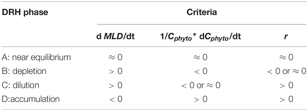
Table 1. Summary of the criteria used to identify the phytoplankton seasonal phenology characteristics described by the Disturbance Recovery Hypothesis (DRH) based on temporal variations of mixed layer depth MLD (entrainment versus shoaling), mixed layer phytoplankton biomass C_phyto, and specific net phytoplankton accumulation rate r from Eq. 4 and 5.

An analysis based on the relationship between dμ/dt and r in the context of DRH (based on Eq. 8 in Behrenfeld and Boss, 2018) was also included in the Supplementary Material.

Results and Discussion

Observed/Modeled Spatial-Temporal Variability in Surface Photosynthetically Active Radiation (PAR_surf) and Mixed Layer Depth (MLD)

Surface Photosynthetically Active Radiation (PAR_surf) and mixed layer depth (MLD) are two important environmental parameters essential for characterizing phytoplankton growth and biomass accumulation. As shown by the satellite data, surface PAR for phytoplankton growth increased from the north to south (Figures 2A, 3A, 4A, 5A), with the PAR_surf seasonal maximum (from 1.5 to 2 mol photon m^–2 h^–1) around May to July (late spring/summer) and the minimum (from 0 to 0.3 mol photon m^–2 h^–1) in January. Only the northernmost D1 region had near-zero PAR_surf in January. The PAR_surf from CESM (estimated as a constant fraction of solar short-wave heat flux) showed similar trends with slightly lower light level in the spring and summer months. For all four regions, MLD from all three approaches started deepening and shoaling around September and March, respectively (Figures 2B, 3B, 4B, 5B). The northernmost D1 region had the deepest winter MLD at about 500 m, while the winter MLD for other regions were around 200 to 300 m. For most of the year the isolume depth (below which light is insufficient for photosynthesis) Z(0.415) was shallower than MLD except for June to September when they were similar. Z(0.415) values increased from north to south as PAR_surf increased.

FIGURE 2

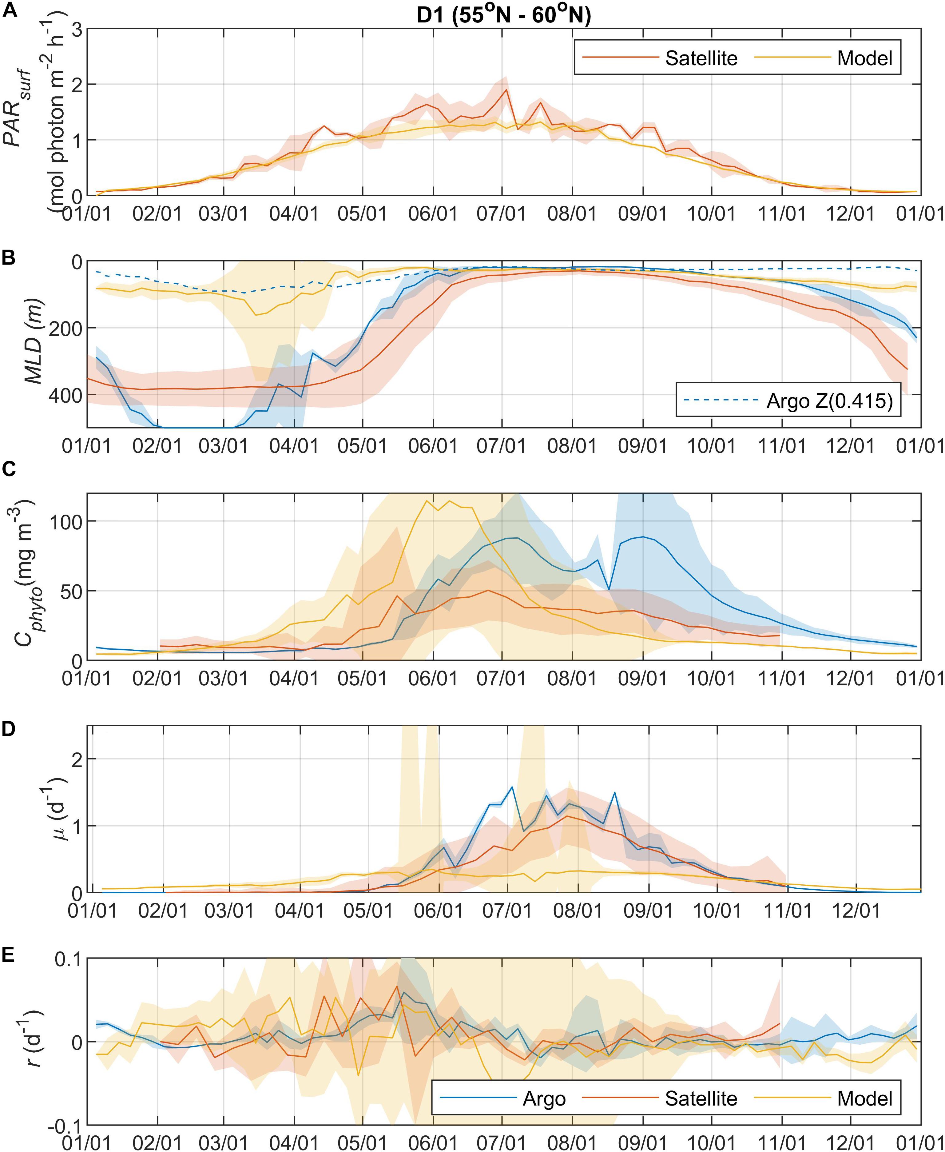
Figure 2. Seasonal climatologies of (A) surface photosynthetically active radiation (PAR_surf), (B) mixed layer depth (MLD, m), (C) mixed layer phytoplankton carbon biomass (C_phyto, mg m^–3), (D) mixed layer phytoplankton specific division rate (μ, d^–1), and (E) mixed layer phytoplankton net accumulation rate (r, d^–1) from Argo floats, satellite, and model simulation (blue: Argo, red: satellite, yellow: model) for region D1 (see map in Figure 1 for region boundaries). Note that the MLD used in satellite algorithm came from HYCOM. The lighter shadings represent one standard deviation. The dashed blue line in panel b represents the isolume depth Z(0.415) derived from Argo measurements (see section “Float Data” for details).

FIGURE 3

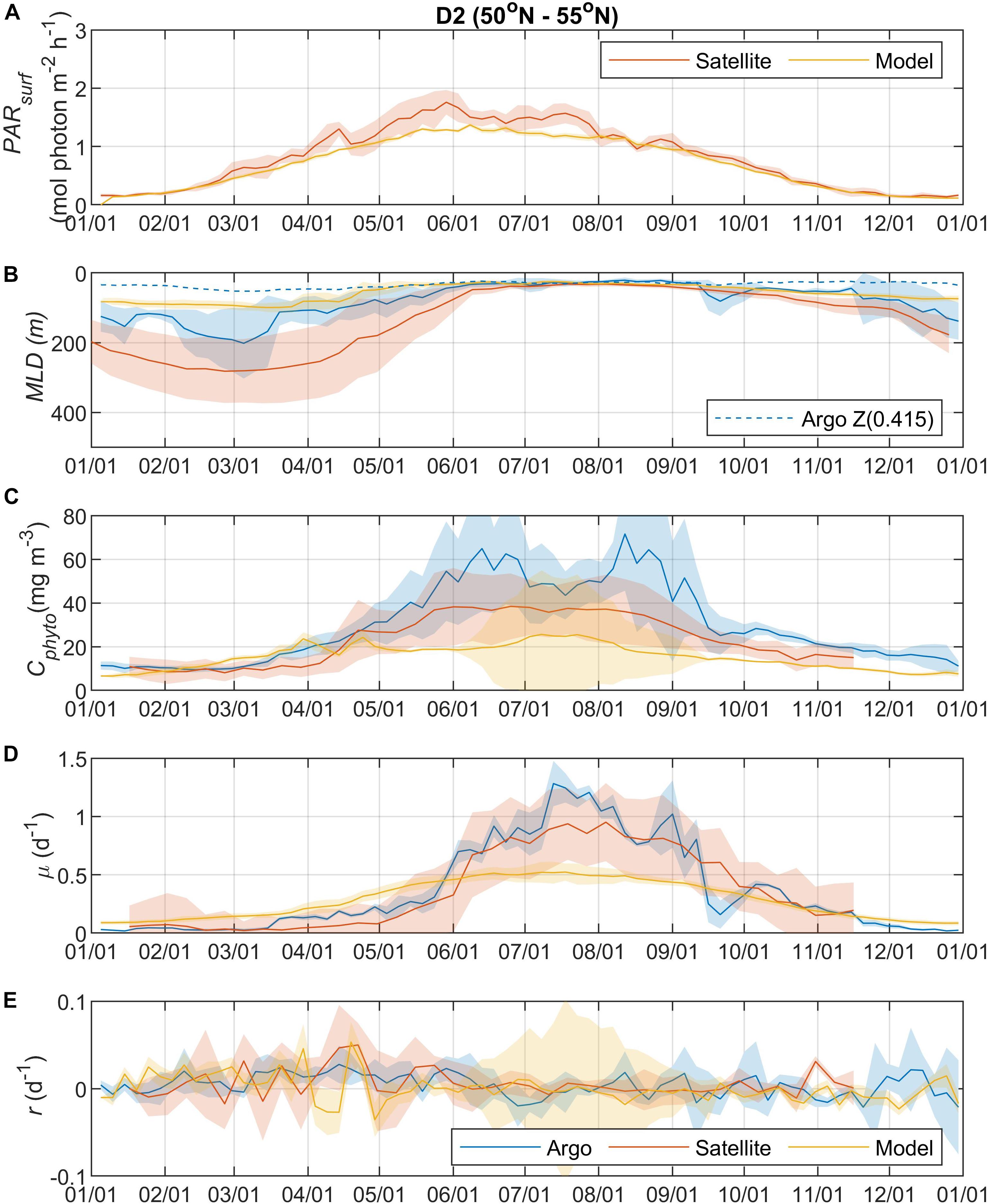
Figure 3. Seasonal climatologies of (A) PAR_surf, (B) MLD, (C) C_phyto, (D) μ, and (E) r from Argo floats, satellite, and model simulation for region D2. See the caption of Figure 2 for details.

FIGURE 4

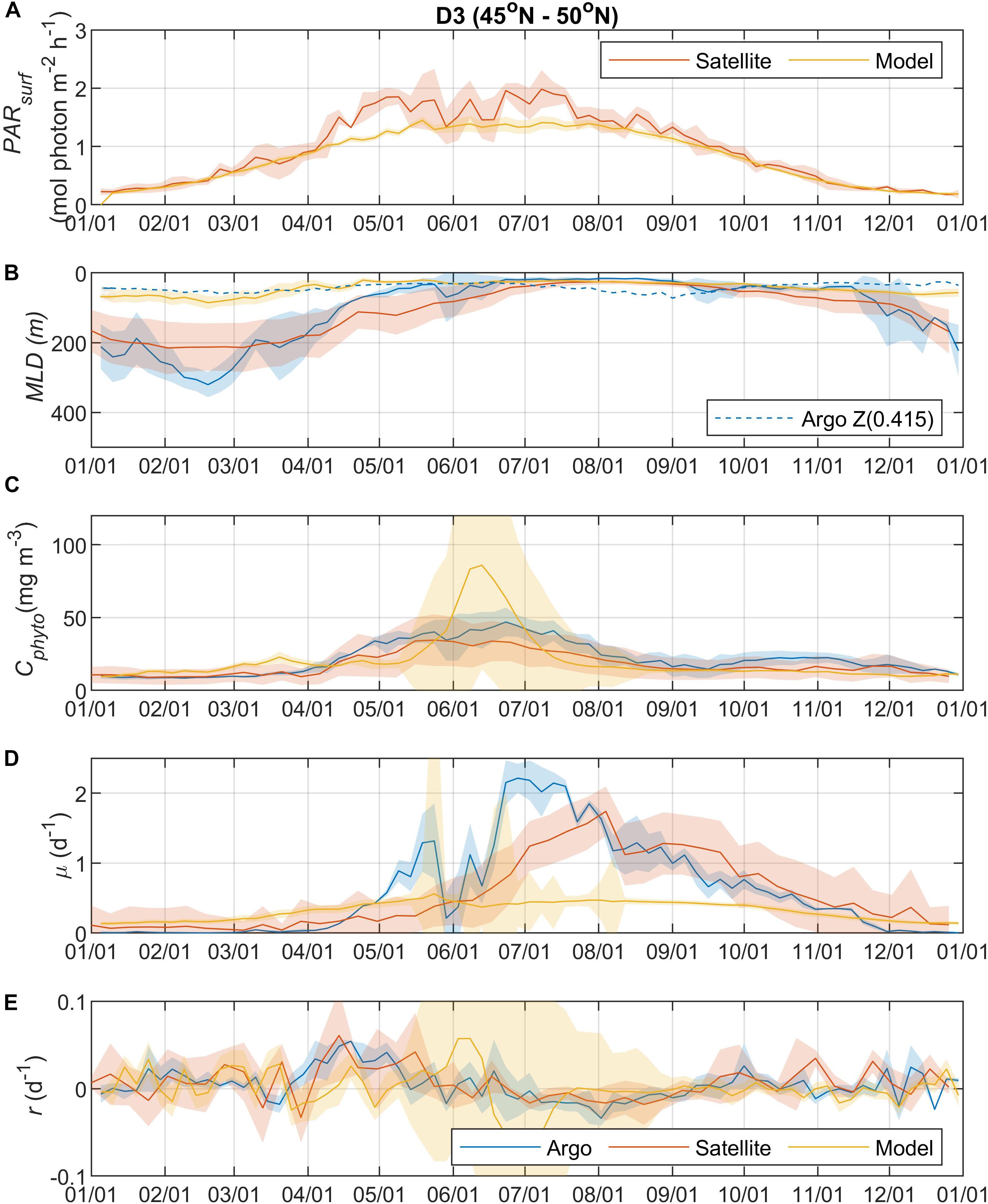
Figure 4. Seasonal climatologies of (A) PAR_surf, (B) MLD, (C) C_phyto, (D) μ, and (E) r from Argo floats, satellite, and model simulation for region D3. See the caption of Figure 2 for details.

FIGURE 5

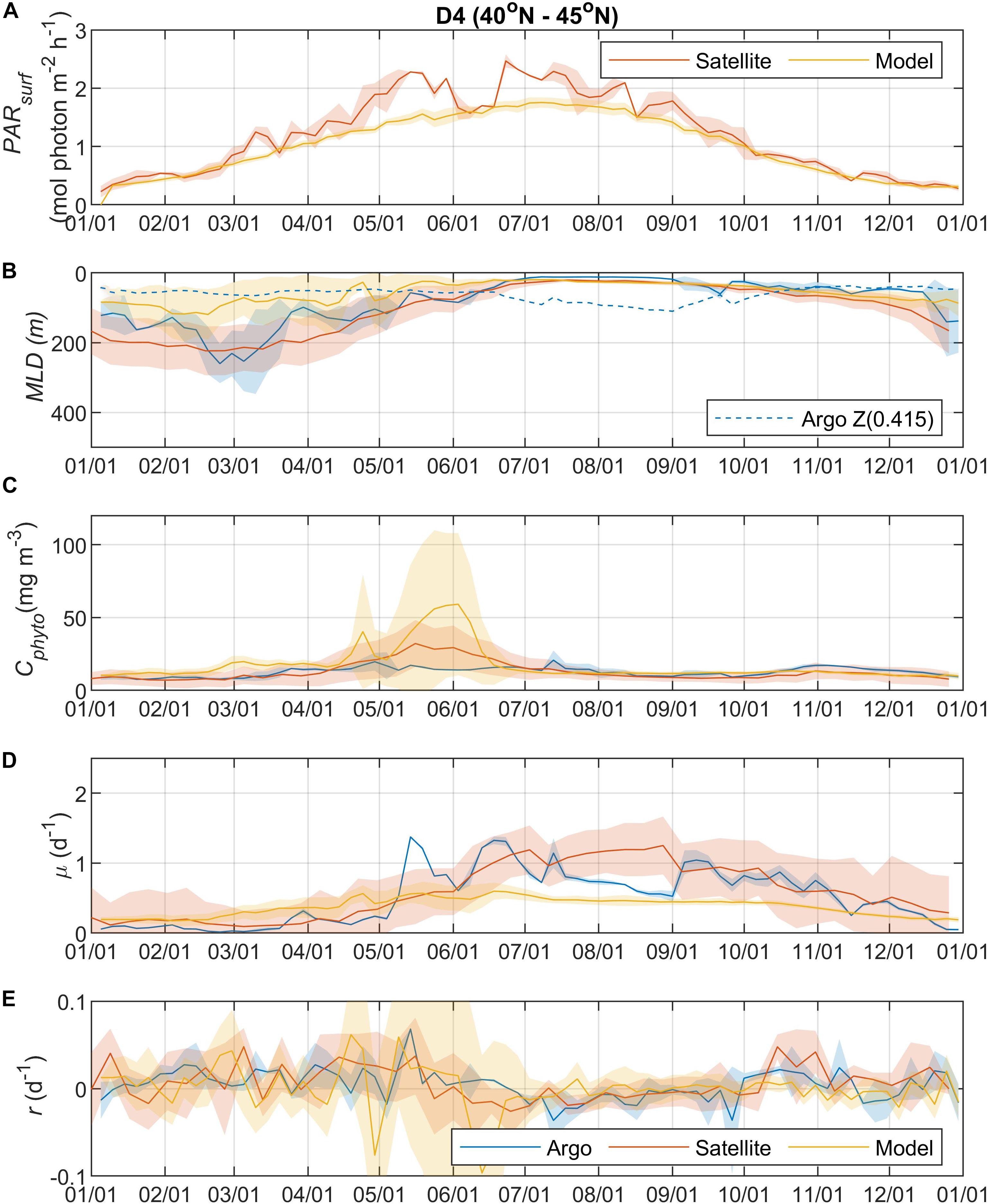
Figure 5. Seasonal climatologies of (A) PAR_surf, (B) MLD, (C) C_phyto, (D) μ, and (E) r from Argo floats, satellite, and model simulation for region D4. See the caption of Figure 2 for details.

The MLD from all three approaches (float, satellite, and model) had similar seasonal patterns and geographic trends, although values from CESM were significantly shallower in the winter. From the perspective of the DRH, the general similarity in the timing of entrainment versus detrainment suggests that all three approaches are capable of capturing the proposed effect of dilution on decoupling production and loss terms, though with weaker magnitude in the model. Model MLD discrepancies in this region have been identified previously and are not unexpected given the complex, regional pattern of deep and shallow winter MLD linked to the positions of the Gulf Stream/North Atlantic Drift and Labrador Current, air-sea fluxes, lateral advection and turbulent mixing, and boundary layer dynamics (Moore et al., 2013; Harrison et al., 2018).

Observed/Modeled Spatial-Temporal Variability in Phytoplankton Carbon Biomass (C_phyto), Growth Rate (μ) and Carbon Accumulation Rate (r)

The overall magnitude of year-round mixed layer C_phyto decreased from the north to the south (Figures 2C, 3C, 4C, 5C, also see Figure 6), with the peak occurring in the summer for the northern regions (D1 and D2) and late spring for the southern regions (D3 and D4). Winter biomass (the inoculum for the spring bloom) made a greater contribution to annual biomass in the southern regions, as the summer/spring C_phyto decreased from north to south while winter C_phyto increased from north to south. As indicated by the standard deviation (light shadings), spatial variations also decreased from north to south, indicating that the northern regions were more dynamic than the southern regions (Glover et al., 2018). In general, the overall magnitude of year-round mixed layer μ increased as latitude decreased and PAR_surf increased (Figures 2D, 3D, 4D, 5D). The peak of μ from the Argo float data occurred earlier at lower latitudes than further north (around August to September for the northernmost region D1, and July for the southernmost region D4), which could be attributed to surface nutrient limitation (Garcia et al., 2013) in the southern regions (surface nutrient depletion in the summer “throttled” phytoplankton growth despite the improved light condition). Similar to μ, the peak in r occurred earlier and with higher positive winter values at lower latitudes (Figures 2E, 3E, 4E, 5E). It should be noted that in several cases both satellite and Argo float data had zero or near-zero chlorophyll readings in the winter (that could due to sensitivity of the optical sensors) while the float backscatter sensors still detected positive signals (that could be from non-phytoplankton contributions, or the uncertainties of the algorithm used to calculated C_phyto from backscattering), which led to positive r values (indicating biomass accumulation) with corresponding μ values being zero or near zero (indicating no growth).

FIGURE 6

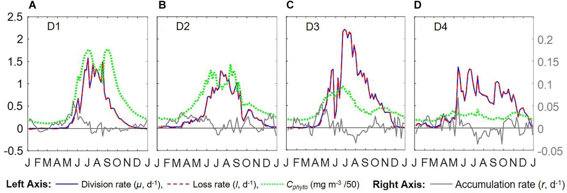
Figure 6. Seasonal climatologies of C_phyto, μ, l, and r from Argo floats for all 4 regions (panels (A–D) represent regions D1–D4). Unit for μ, l, and r is d^–1.

Comparisons Between Argo, Satellite Remote Sensing, and Model Results

Overall, the Argo float-derived C_phyto, μ, and r were very comparable (in both seasonality and magnitude) with the satellite-derived counterparts. For C_phyto, the Argo and satellite results showed good agreement except for the northernmost D1 region with higher float C_phyto. The μ values from Argo floats and satellite observations had similar temporal trends and magnitudes, with the Argo floats indicating higher μ (than satellite) from May to August for all 4 regions and the satellite-derived μ showing higher values (than Argo float) from August to October for the southern regions D3 and D4. r derived from Argo measurements agreed well with the satellite remote sensing observations. The small discrepancies between satellite and Argo approaches for C_phyto, μ, and r were most likely due to differences between Argo and satellite spatial and temporal coverage (see section “Construction of Regional, Climatological Patterns in Bloom Phenology”).

The comparison results between the CESM model simulation and Argo/satellite approaches were more complicated. The model did capture most of the seasonal variations in C_phyto, but with significant difference in magnitude during the periods when C_phyto was high (e.g., modeled early summer C_phyto was lager in D1, D3, and D4 than the Argo/satellite results, but smaller in D2). Because the modeled C_phyto had similar temporal trends to the Argo/satellite results in all four regions, the modeled r (derived from modeled C_phyto) did reproduce most aspects of the seasonal phenology shown by the Argo/satellite approaches, such as weak (but positive) biomass accumulation in the winter, increased biomass accumulation rate in the spring, near-equilibrium (r ≈ 0) in late summer or fall, and the depletion phase after that. The largest discrepancy between model and Argo/satellite results was in the division rate μ. The modeled μ were similar in all four regions with values between 0.1 and 0.5 d^–1 and peak values in the summer, which were different from the Argo and satellite results. Such differences in the magnitude of C_phyto and the trend/magnitude of μ could be attributed to potential model biases in the formulation of phytoplankton growth and loss terms and/or the different physical forcing used in the model, or systematic differences due to the productivity models used in the Argo/Satellite approaches. The attribution of causes of the model biases identified here could result from various model physical and biogeochemical deficiencies that are beyond the scope of the current study, which is focused primarily on float data. The identified model biases will be investigated in future studies that focus in more detail on the simulation dynamics.

Mixed Layer Phytoplankton Phenology Based on Argo Observations

Overall, the year-round variations of μ, r, l, and C_phyto for all four regions from the Argo data (Figure 6) were very similar to Figure 5f from Behrenfeld and Boss (2018) for the DRH scenario. Our analysis of seasonal variations in phytoplankton phenology starts from the pre-bloom conditions in late fall and winter. Despite the low light level (PAR_surf), decreasing μ, and deepening MLD, positive r (phytoplankton biomass accumulation rate, gray lines in Figures 6A–D) started to appear around November for all four regions. Furthermore, the magnitude of positive r was larger in the southern regions (40° N – 55° N, D2 – D4) than in the northern region (55° N –60° N). These findings complement previous Argo observations in the northern region above 48° N (Boss and Behrenfeld, 2010; Mignot et al., 2018). Overall, the observed winter phytoplankton biomass accumulation in November and December was consistent with the disturbance recovery hypothesis (DRH), which states that deep winter mixing is important for the North Atlantic bloom initiation as it reduces the encounter rate between phytoplankton and grazers (“top-down” process).

From January to March, the Argo observations showed low signals of μ (zero or small positive values, blue lines in Figures 6A–D), which could suggest either (1) such a signal was too weak to be captured by Argo measurements or (2) μ was derived from bio-optical parameters and empirical relationships rather than direct measurements, and such relationships may not hold for all seasons and regions. Positive r values were observed in winter by the Argo measurements in all four regions. For the D1 region, a significant positive r signal was found in early January that subsequently decreased to near-zero until March. For regions D2 to D4, r stayed positive throughout this period but fluctuated significantly in magnitude. Such fluctuating patterns indicated that phytoplankton dynamics in late winter/early spring could be the combined result of periodic reductions in grazing (“top-down” process) due to deepening MLD and periodic increases in phytoplankton growth (increasing μ, “bottom-up” process) from improved light conditions (increasing PAR_surf and MLD shoaling with episodic stratification events). Thus, the Argo float data may be consistent, on different time and space-scales, with the disturbance recovery hypothesis over seasonal time-scales as well as other bloom hypotheses, such as the critical turbulence hypothesis that highlights the importance during the late winter/early spring transition of brief, episodic boundary layer shoaling for decoupling of division and grazing rates (Fischer et al., 2014).

From March to June, MLD shoaled rapidly and surface light increased continually. μ continued to increase throughout this period in all four regions, while r fluctuated between positive and negative values. Such coupling/decoupling patterns of μ and r indicated the interplay of “bottom-up” (increase in phytoplankton growth due to improved environmental conditions) and “top-down” (increase in grazing due to the shoaling MLD) controls of phytoplankton dynamics, consistent with patterns described by DRH.

After May/June, r started dropping as the mixed layer continued shoaling and stratification increased, with values approaching zero despite the continuously increasing μ. Such decoupling of μ and r also supports the DRH in which near-equilibrium conditions prevail over the stratified summer period, when μ and l are in approximate balance. After August, both μ and r decreased as the mixed layer deepened and light levels decreased. This “depletion phase” (r < 0) is a result of lags in the relationship between phytoplankton loss rates and division rates (Behrenfeld and Boss, 2018).

With the criteria listed in Table 1, we identified the DRH phases for each region based on the Argo float data, with the results presented in Figure 7 as color-coded, shaded bars for each identified phase (periods that did not meet all three criteria were left blank). The four different DRH phases could be identified in all four regions along the north-south transect. The summer near-equilibrium phase (phase A) arrived earlier for the lower latitude regions and, for most cases, values of 1/C_phyto^∗d C_phyto/dt and r fluctuated between positive and negative rather than staying around zero for the whole phase. All regions except D1 had a period with positive r (fall bloom) during the fall depletion phase (phase B), which could be the result of some weak dilution effect or enhanced nutrient supply from deep mixing. For the northern regions (D1, D2), the spring accumulation phase (phase D) was longer and contributed more to the annual biomass accumulation, while in the southern regions (D3, D4) the accumulation phase was shorter and the biomass accumulation during the dilution phase (phase C) contributed more to the annual biomass accumulation.

FIGURE 7

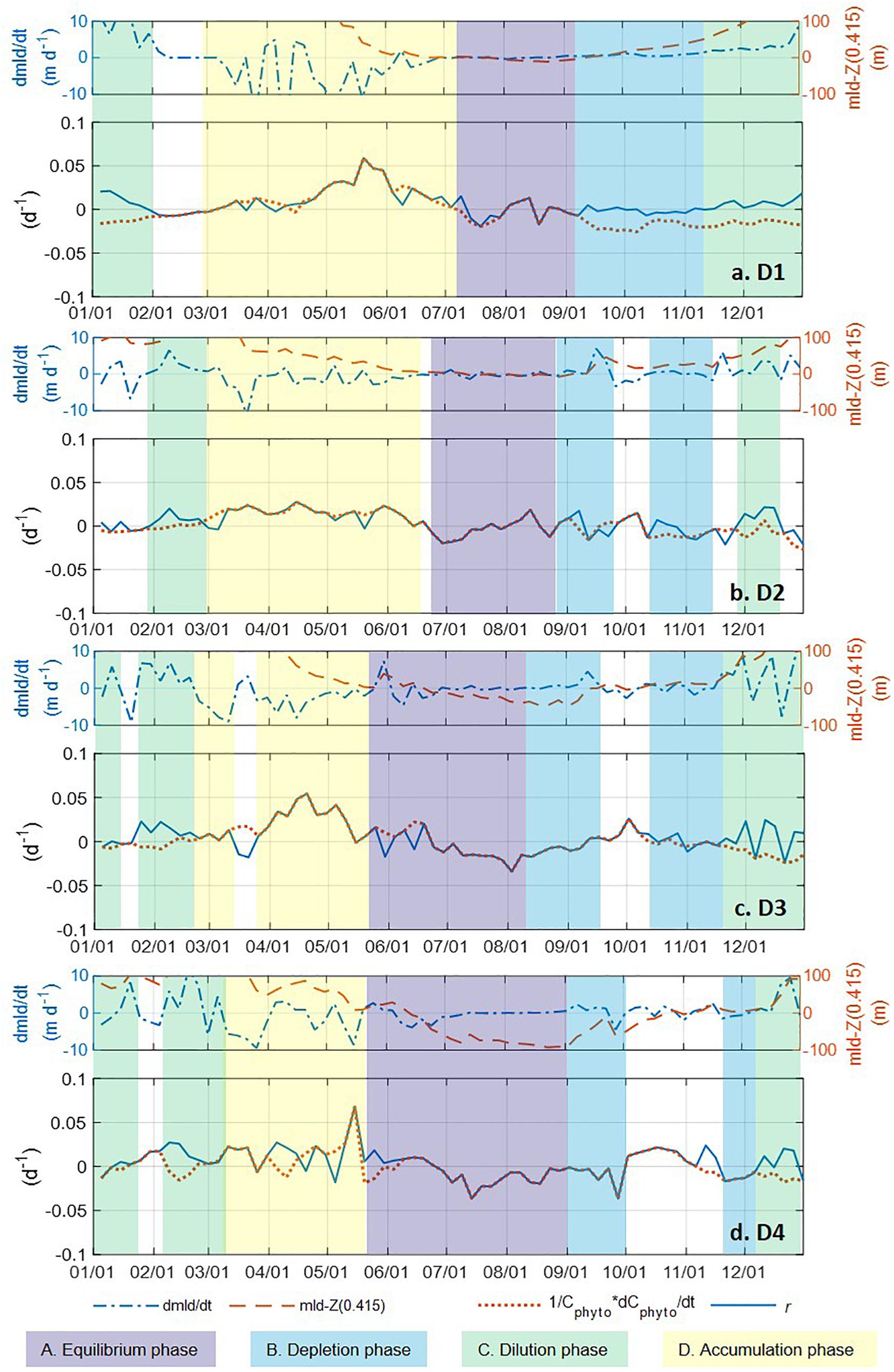
Figure 7. The time rate of change in MLD (d MLD/dt, blue dash-dotted line), difference between MLD and Z(0.415) (red dashed line), time rate of change in normalized C_phyto (1/C_phyto*d C_phyto/dt, red dotted line), and phytoplankton net accumulation rate r (blue solid line) in the mixed layer from biogeochemical Argo float measurements (panels A–D represent regions D1–D4). A five-point moving mean was applied to all three parameters. The color shadings represent the four phases of the seasonal phytoplankton biomass dynamics described by the “Disturbance and Recovery Hypothesis (DRH)”. Periods with phytoplankton phenology that did not have all the characteristics matching any DRH phase were left blank, without any color shading.

Implications From Vertical Distribution of Phytoplankton Carbon Production

Previous studies (e.g., Lacour et al., 2017, 2019) have shown that vertical distributions of Chl and b_bp did not always tightly track the density-based MLD. In this study, although the Chl and C_phyto (derived from b_bp) profiles were mostly consistent with the MLD and/or Z(0.415) isolume depth, mismatches were also observed (especially during the winter-spring transition period, Supplementary Figures S5, S6). Therefore, for such periods the estimations of r from the sum of biomass over the density-based MLD or isolume depth can be biased, and the depth profile of r would provide a better metric. We used Argo-derived monthly depth profiles of specific net phytoplankton accumulation rates r from the northernmost D1 region (Figure 8C), as an example, to explore the vertical structures of phytoplankton carbon production within and below the density-based mixed layer, as well as to investigate controls on the North Atlantic phytoplankton bloom.

FIGURE 8

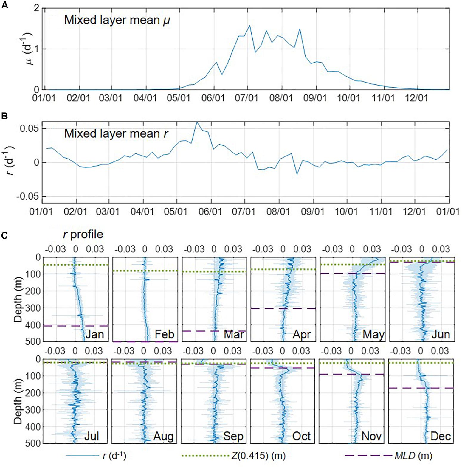
Figure 8. (A,B) Seasonal climatologies of mixed layer mean μ, and r for region D1. (C) Monthly climatologies of specific net phytoplankton accumulation rates (r) profiles derived from Argo profiling floats (standard deviation indicated with the shading) in. The green dotted line and purple dash line indicated isolume depth Z(0.415) and mixed layer depth (MLD), respectively.

One of the key characteristics of the DRH is that winter biomass accumulation will occur from the dilution effect (deep mixing reduced loss rate), which has been found by some Argo-based studies (e.g., Boss and Behrenfeld, 2010; Mignot et al., 2014). However, the recent glider-based study by Rumyantseva et al. (2019) did not show any significant biomass accumulation from December to the end of January. Our Argo float observations clearly showed biomass accumulation averaged over the mixed layer (positive r, Figure 8B) during the winter period in November, December, and January, when the mixed layer continued deepening and division rate μ was very low or near zero (Figure 8A). The vertical profiles of r derived from the float observations for these 3 months showed substantial depth variations, with negative or near zero r in the upper part of the mixed layer and higher and positive r in the lower part of the mixed layer and just below the mixed layer (Figure 8C). During the late-fall and winter period, mixed layer deepening (entrainment) acts to transport biomass downward into the eroding seasonal thermocline depth zone that previously had very low biomass because of respiration over the summer. Surface biomass concentration may remain flat, but the downward physical transport and build-up of biomass at depth causes positive r for the vertically integrated phytoplankton population.

Some previous Argo/glider based studies (e.g., Lacour et al., 2017; Rumyantseva et al., 2019) found that ephemeral shallow mixing due to horizontal density gradients and relaxation of atmospheric forcing may trigger the phytoplankton bloom during the winter/spring transition (February and March) [see also Fischer et al. (2014) for summary of other observational and modeling bloom dynamics studies]. In our case, the mixed layer mean r was slightly negative (Figure 8B), showing no biomass accumulation in February. Specifically, r in the upper part of the mixed layer was slightly higher than in January (the division rate μ could increase due to higher light level, but the signal might be too weak to show in Figure 8A) but still around zero, the r values in the deeper part of the mixed layer (200 – 500 m) decreased, and positive r was only found between 350 to 500 m (Figure 8C). In March the biomass accumulation rate (r) increased significantly within the mixed layer, especially in the well-lit layer above Z(0.415) (Figure 8C), resulting in the increase of mixed layer mean r (Figure 8B). Although the float μ signals (Figure 8A) were still weak, increased Chl-a was observed in the upper part of the mixed layer (Supplementary Figure S5), which could indicate elevated division rate in the upper part of the mixed layer and that ephemeral shallow mixing may be involved to some extent. Overall the increased biomass accumulation rate in March was most likely due to the acceleration in division rate.

From March to the end of May as mixed layer μ increased (Figure 8A), the biomass accumulation rate (r) increased significantly at all depths within the mixed layer, especially in the well-lit upper part of the mixed layer, and was near zero or slightly negative below the mixed layer (Figure 8C). During this period of time, the biomass accumulation rate within the mixed layer decreased with depth, indicating that deceleration in division rate (i.e., due to decreased light) was likely a major control of the biomass accumulation. Surface warming could also lead to enhanced division rates, μ, in nutrient replete conditions. In June, mixed layer μ continued to increase (Figure 8A) while mixed layer r started to decrease (Figure 8B). Vertically, values of r in the upper part of the mixed layer were still higher than the lower part of the mixed layer (Figure 8C). Such decoupling of mixed layer μ and r could be due to enhanced losses in the stratified shallow MLD as zooplankton biomass catches up with phytoplankton biomass (Behrenfeld et al., 2013). These effects caused r to continue to decrease in July and August while μ remained relatively stable, which led to an “equilibrium phase” in the mixed layer (mean r in the mixed layer close to zero) and below the mixed layer (r fluctuating between positive and negative). After August, the decreasing μ indicated the start of the “depletion phase”. In September, mixed layer r reached its lowest value for the year, while r values below the mixed layer were positive and higher than those in August. From October to December, the mixed layer continued deepening and r in the mixed layer increased during these 3 months, with lower values in the surface and higher values at the lower part of the mixed layer, which was consistent with DRH (deep mixing promoted biomass accumulation rate in the winter by reducing grazing). Biomass accumulation rate also increased below the mixed layer, indicating carbon export into the deep ocean.

Summary

In this work, we used results from biogeochemical Argo float measurements to analyze seasonal phytoplankton phenology of the western temperate and sub-polar North Atlantic along a north-south transect (40° N to 60° N). Our results are broadly consistent with the general framework of the Disturbance Recovery Hypothesis (DRH) over the seasonal time-scale, where slight imbalances between division (μ) and loss (l) govern seasonal phytoplankton dynamics. All four phases described by DRH could be identified from Argo float-based phytoplankton metrics. The annual phytoplankton biomass (C_phyto) decreased significantly from north to the south, with the C_phyto peak appearing earlier in the year in the southern region than in the northern region. As for the phytoplankton specific carbon accumulation rate (r), positive values (indicating biomass accumulation) were found in all four regions during the winter (November to January) due to the decoupling of division rate (μ) and loss rate (l), which was most likely due to the dilution effect of deep mixing that reduced the encounter rate of phytoplankton and zooplankton. From north to south, the winter biomass accumulation period became more important for the annual biomass accumulation, as indicated by both C_phyto and r. The float results of phytoplankton phenology in the mixed layer were comparable to the ocean color satellite remote sensing observations. An eddy-resolving model simulation reproduced most of the bloom characteristics shown by Argo and satellite, despite the differences in the physical forcing/turbulent dynamics and potential model biases. The Argo float data provide an important, complementary approach to satellite remote sensing for high-resolution observation and regions with high solar zenith angles or obscured by clouds. Furthermore, the depth profiling capacity of Argo floats provided information on the vertical distribution of phytoplankton carbon production. As in situ measurement techniques like biogeochemical Argo floats and ship-board underway measurements continue to improve and field observations of phytoplankton phenology increase, it will be possible to verify satellite- and model-based estimates of phytoplankton dynamics to gain further insight into factors that control phytoplankton blooms in different marine biogeographic regimes.

Data Availability Statement

The float data is available at: http://misclab.umeoce.maine.edu/floats/, as well as http://biogeochemical-argo.org/. The satellite data is available at: http://www.science.oregonstate.edu/ocean.productivity/index.php. The outputs from CESM simulation are available on request to the corresponding author.

Author Contributions

BY, RE, MB, and SD designed the experiments and analyzed the data. EB and NH were in charge of Argo float deployments and raw data processing. ML preformed the CESM model simulation. BY and SD prepared the manuscript with contributions from all co-authors.

Funding

Support for this work came from the National Aeronautics and Space Administration (NASA) as part of the North Atlantic Aerosol and Marine Ecosystems Study (NAAMES, grants NNX15AF30G, 80NSSC18K0018, and NNX15AE67G). The CESM project was supported by the National Science Foundation and the Office of Science (BER) of the United States Department of Energy. Computing resources were provided by the Climate Simulation Laboratory at NCAR’s Computational and Information Systems Laboratory (CISL), sponsored by the National Science Foundation and other agencies. This research was enabled by CISL compute and storage resources.

Conflict of Interest

The authors declare that the research was conducted in the absence of any commercial or financial relationships that could be construed as a potential conflict of interest.

The reviewer CN declared a past co-authorship, with one of the authors ML to the handling Editor.

Acknowledgments

The authors gratefully acknowledge the efforts of all the science party and crew during the NAAMES campaigns.

Supplementary Material

The Supplementary Material for this article can be found online at: https://www.frontiersin.org/articles/10.3389/fmars.2020.00139/full#supplementary-material

Footnotes

1. ^ https://naames.larc.nasa.gov/
2. ^ http://orca.science.oregonstate.edu/1080.by.2160.8day.hdf.cbpm2.m.php
3. ^ http://sites.science.oregonstate.edu/ocean.productivity/1080.by.2160.monthly.inputData.php

References

Behrenfeld, M. J. (2010). Abandoning sverdrup’s critical depth hypothesis on phytoplankton blooms. Ecology 91, 977–989. doi: 10.1890/09-1207.1

PubMed Abstract | CrossRef Full Text | Google Scholar

Behrenfeld, M. J., Boss, E., Siegel, D. A., and Shea, D. M. (2005). Carbon-based ocean productivity and phytoplankton physiology from space. Global Biogeochem. Cycles 19:GB1006. doi: 10.1029/2004GB002299

CrossRef Full Text | Google Scholar

Behrenfeld, M. J., and Boss, E. S. (2013). Resurrecting the ecological underpinnings of ocean plankton blooms. Ann. Rev. Mar. Sci. 6, 167–194. doi: 10.1146/annurev-marine-052913-021325

PubMed Abstract | CrossRef Full Text | Google Scholar

Behrenfeld, M. J., and Boss, E. S. (2018). Student’s tutorial on bloom hypotheses in the context of phytoplankton annual cycles. Glob. Chang. Biol. 24, 55–77. doi: 10.1111/gcb.13858

PubMed Abstract | CrossRef Full Text | Google Scholar

Behrenfeld, M. J., Doney, S. C., Lima, I., Boss, E. S., and Siegel, D. A. (2013). Annual cycles of ecological disturbance and recovery underlying the subarctic Atlantic spring plankton bloom. Global Biogeochem. Cycles 27, 526–540. doi: 10.1002/gbc.20050

CrossRef Full Text | Google Scholar

Behrenfeld, M. J., Moore, R. H., Hostetler, C. A., Graff, J., Gaube, P., Russell, L. M., et al. (2019). The north atlantic aerosol and marine ecosystem study (NAAMES): science motive and mission overview. Front. Mar. Sci. 6:122. doi: 10.3389/fmars.2019.00122

CrossRef Full Text | Google Scholar

Boss, E., and Behrenfeld, M. (2010). In situ evaluation of the initiation of the North Atlantic phytoplankton bloom. Geophys. Res. Lett. 37:L18603. doi: 10.1029/2010GL044174

CrossRef Full Text | Google Scholar

Cetinić, I., Perry, M. J., D’Asaro, E., Briggs, N., Poulton, N., Sieracki, M. E., et al. (2015). A simple optical index shows spatial and temporal heterogeneity in phytoplankton community composition during the 2008 North Atlantic Bloom Experiment. Biogeosciences 12, 2179–2194. doi: 10.5194/bg-12-2179-2015

CrossRef Full Text | Google Scholar

Chiswell, S. M., Calil, P. H. R., and Boyd, P. W. (2015). Spring blooms and annual cycles of phytoplankton: a unified perspective. J. Plankton Res. 37, 500–508. doi: 10.1093/plankt/fbv021

CrossRef Full Text | Google Scholar

Dale, T., Rey, F., and Heimdal, B. R. (1999). Seasonal development of phytoplankton at a high latitude oceanic site. Sarsia 84, 419–435. doi: 10.1080/00364827.1999.10807347

CrossRef Full Text | Google Scholar

de Boyer Montégut, C. (2004). Mixed layer depth over the global ocean: an examination of profile data and a profile-based climatology. J. Geophys. Res. 109:C12003. doi: 10.1029/2004JC002378

CrossRef Full Text | Google Scholar

Evans, G. T., and Parslow, J. S. (1985). A model of annual plankton cycles. Deep Sea Res. Part B. Oceanogr. Lit. Rev. 3, 327–347. doi: 10.1016/0198-0254(85)92902-4

CrossRef Full Text | Google Scholar

Fischer, A., Moberg, E., Alexander, H., Brownlee, E., Hunter-Cevera, K., Pitz, K., et al. (2014). Sixty Years of Sverdrup: a retrospective of progress in the study of phytoplankton blooms. Oceanography 27, 222–235. doi: 10.5670/oceanog.2014.26

CrossRef Full Text | Google Scholar

Garcia, H. E., Locarnini, R. A., Boyer, T. P., Antonov, J. I., Baranova, O. K., Zweng, M. M., et al. (2013). World Ocean Atlas 2013, Volume 4: dissolved Inorganic Nutrients (phosphate, nitrate, silicate). Noaa Atlas Nesdis 76:25. doi: 10.1182/blood-2011-06-357442

PubMed Abstract | CrossRef Full Text | Google Scholar

Glover, D. M., Doney, S. C., Oestreich, W. K., and Tullo, A. W. (2018). Geostatistical analysis of mesoscale spatial variability and error in seawifs and modis/aqua global ocean color data. J. Geophys. Res. Ocean. 123, 22–39. doi: 10.1002/2017JC013023

CrossRef Full Text | Google Scholar

Graff, J. R., Westberry, T. K., Milligan, A. J., Brown, M. B., Dall’Olmo, G., van Dongen-Vogels, V., et al. (2015). Analytical phytoplankton carbon measurements spanning diverse ecosystems. Deep. Res. Part I Oceanogr. Res. Pap. 102, 16–25. doi: 10.1016/j.dsr.2015.04.006

CrossRef Full Text | Google Scholar

Gran, H. H., and Braarud, T. (1935). A quantitative study of the phytoplankton in the bay of fundy and the gulf of maine (including observations on hydrography, chemistry and turbidity). J. Biol. Board Canada 1, 279–467. doi: 10.1139/f35-012

CrossRef Full Text | Google Scholar

Harrison, C. S., Long, M. C., Lovenduski, N. S., and Moore, J. K. (2018). mesoscale effects on carbon export: a global perspective. Global Biogeochem. Cycles 32, 680–703. doi: 10.1002/2017GB005751

CrossRef Full Text | Google Scholar

Hashioka, T., Vogt, M., Yamanaka, Y., Le Quéré, C., Buitenhuis, E. T., Aita, M. N., et al. (2013). Phytoplankton competition during the spring bloom in four plankton functional type models. Biogeosciences 10, 6833–6850. doi: 10.5194/bg-10-6833-2013

CrossRef Full Text | Google Scholar

Huisman, J., Van Oostveen, P., and Weissing, F. J. (1999). Critical depth and critical turbulence: two different mechanisms for the development of phytoplankton blooms. Limnol. Oceanogr. 44, 1781–1787. doi: 10.4319/lo.1999.44.7.1781

CrossRef Full Text | Google Scholar

Hurrell, J. W., Holland, M. M., Gent, P. R., Ghan, S., Kay, J. E., Kushner, P. J., et al. (2013). The community earth system model: a framework for collaborative research. Bull. Am. Meteorol. Soc. 94, 1339–1360. doi: 10.1175/BAMS-D-12-00121.1

CrossRef Full Text | Google Scholar

Lacour, L., Ardyna, M., Stec, K. F., Claustre, H., Prieur, L., Poteau, A., et al. (2017). Unexpected winter phytoplankton blooms in the North Atlantic subpolar gyre. Nat. Geosci. 10, 836–839. doi: 10.1038/NGEO3035

CrossRef Full Text | Google Scholar

Lacour, L., Briggs, N., Claustre, H., Ardyna, M., and Dall’Olmo, G. (2019). The intraseasonal dynamics of the mixed layer pump in the subpolar north atlantic ocean: a biogeochemical-argo float approach. Global Biogeochem. Cycles 33, 266–281. doi: 10.1029/2018GB005997

CrossRef Full Text | Google Scholar

Letelier, R. M., Karl, D. M., Abbott, M. R., and Bidigare, R. R. (2004). Light driven seasonal patterns of chlorophyll and nitrate in the lower euphotic zone of the North Pacific Subtropical Gyre. Limnol. Oceanogr. 49, 508–519. doi: 10.4319/lo.2004.49.2.0508

CrossRef Full Text | Google Scholar

Longhurst, A. R. (2007). “Toward an ecological geography of the sea,” in Ecological Geography of the Sea (San Diego: Academic Press), 1–17.

Google Scholar

Mahadevan, A. (2016). The impact of submesoscale physics on primary productivity of plankton. Ann. Rev. Mar. Sci. 8, 161–184. doi: 10.1146/annurev-marine-010814-015912

PubMed Abstract | CrossRef Full Text | Google Scholar

Mahadevan, A., D’Asaro, E., Lee, C., and Perry, M. J. (2012). Eddy-driven stratification initiates North Atlantic spring phytoplankton blooms. Science 337, 54–58. doi: 10.1126/science.1218740

PubMed Abstract | CrossRef Full Text | Google Scholar

Mignot, A., Claustre, H., Uitz, J., Poteau, A., D’Ortenzio, F., and Xing, X. (2014). Understanding the seasonal dynamics of phytoplankton biomass and the deep chlorophyll maximum in oligotrophic environments: a Bio-Argo float investigation. Global Biogeochem. Cycles 28, 856–876. doi: 10.1002/2013GB004781

CrossRef Full Text | Google Scholar

Mignot, A., Ferrari, R., and Claustre, H. (2018). Floats with bio-optical sensors reveal what processes trigger the North Atlantic bloom. Nat. Commun. 9, 190. doi: 10.1038/s41467-017-02143-6

PubMed Abstract | CrossRef Full Text | Google Scholar

Moore, J. K., Lindsay, K., Doney, S. C., Long, M. C., and Misumi, K. (2013). Marine ecosystem dynamics and biogeochemical cycling in the community earth system model [CESM1(BGC)]: comparison of the 1990s with the 2090s under the RCP4.5 and RCP8.5 Scenarios. J. Clim. 26, 9291–9312. doi: 10.1175/JCLI-D-12-00566.1

CrossRef Full Text | Google Scholar

Morel, A., and Maritorena, S. (2001). Bio-optical properties of oceanic waters: a reappraisal. J. Geophys. Res. Ocean. 106, 7163–7180. doi: 10.1029/2000JC000319

CrossRef Full Text | Google Scholar

Obata, A., Ishizaka, J., and Endoh, M. (1996). Global verification of critical depth theory for phytoplankton bloom with climatological in situ temperature and satellite ocean color data. J. Geophys. Res. C Ocean 101, 20657–20667. doi: 10.1029/96JC01734

CrossRef Full Text | Google Scholar

Rumyantseva, A., Henson, S., Martin, A., Thompson, A. F., Damerell, G. M., Kaiser, J., et al. (2019). Phytoplankton spring bloom initiation: the impact of atmospheric forcing and light in the temperate North Atlantic Ocean. Prog. Oceanogr. 178:102202. doi: 10.1016/j.pocean.2019.102202

CrossRef Full Text | Google Scholar

Schallenberg, C., Harley, J. W., Jansen, P., Davies, D. M., and Trull, T. W. (2019). Multi-Year observations of fluorescence and backscatter at the Southern Ocean Time Series (SOTS) shed light on two distinct seasonal bio-optical regimes. Front. Mar. Sci. 6:595. doi: 10.3389/fmars.2019.00595

CrossRef Full Text | Google Scholar

Siegel, D. A., Doney, S. C., and Yoder, J. A. (2002). The North Atlantic spring phytoplankton bloom and Sverdrup’s critical depth hypothesis. Science 296, 730–733. doi: 10.1126/science.1069174

PubMed Abstract | CrossRef Full Text | Google Scholar

Smetacek, V., and Passow, U. (1990). Spring bloom initiation and Sverdrup’s critical-depth model. Limnol. Oceanogr. 35, 228–234. doi: 10.4319/lo.1990.35.1.0228

CrossRef Full Text | Google Scholar

Smith, R., Jones, P., Briegleb, B., Bryan, F., Danabasoglu, G., Dennis, J., et al. (2010). “The parallel ocean program (POP) reference manual,”in Ocean Component Of The Community Climate System Model (CCSM). Los Alamos, NM: Los Alamos National Laboratory.

Google Scholar

Sverdrup, H. U. (1953). On conditions for the vernal blooming of phytoplankton. J. Cons. Int. Explor. Mer. 18, 287–295. doi: 10.1093/icesjms/18.3.287

CrossRef Full Text | Google Scholar

Takahashi, T., Sutherland, S. C., Wanninkhof, R., Sweeney, C., Feely, R. A., Chipman, D. W., et al. (2009). Climatological mean and decadal change in surface ocean pCO2, and net sea-air CO2flux over the global oceans. Deep. Res. Part II Top. Stud. Oceanogr. 56, 554–577. doi: 10.1016/j.dsr2.2008.12.009

CrossRef Full Text | Google Scholar

Taylor, J. R., and Ferrari, R. (2011a). Ocean fronts trigger high latitude phytoplankton blooms. Geophys. Res. Lett. 38:L23601. doi: 10.1029/2011GL049312

CrossRef Full Text | Google Scholar

Taylor, J. R., and Ferrari, R. (2011b). Shutdown of turbulent convection as a new criterion for the onset of spring phytoplankton blooms. Limnol. Oceanogr. 56, 2293–2307. doi: 10.4319/lo.2011.56.6.2293

CrossRef Full Text | Google Scholar

Westberry, T., Behrenfeld, M. J., Siegel, D. A., and Boss, E. (2008). Carbon-based primary productivity modeling with vertically resolved photoacclimation. Global Biogeochem. Cycles 22:GB2024. doi: 10.1029/2007GB003078

CrossRef Full Text | Google Scholar

Yoder, J. A., and Kennelly, M. A. (2003). Seasonal and ENSO variability in global ocean phytoplankton chlorophyll derived from 4 years of SeaWiFS measurements. Global Biogeochem. Cycles 17:1112. doi: 10.1029/2002gb001942

CrossRef Full Text | Google Scholar