Hydrodynamics of a Rising Oil Droplet With Bacterial Extracellular Polymeric Substance (EPS) Streamers Using a Microfluidic Microcosm

White, Andrew R.; Jalali, Maryam; Sheng, Jian

doi:10.3389/fmars.2020.00294

ORIGINAL RESEARCH article

Front. Mar. Sci., 06 May 2020
Sec. Marine Ecosystem Ecology
Volume 7 - 2020 | https://doi.org/10.3389/fmars.2020.00294

Hydrodynamics of a Rising Oil Droplet With Bacterial Extracellular Polymeric Substance (EPS) Streamers Using a Microfluidic Microcosm

Andrew R. White

Maryam Jalali

Jian Sheng^*

Department of Engineering, Texas A&M University-Corpus Christi, Corpus Christi, TX, United States

During the Deepwater Horizon oil spill, the unprecedented injection of millions of liters of chemical dispersant at the wellhead generated large quantities of submillimeter oil droplets that became entrained in a deep sea plume. The unexpected generation of these droplets has resulted in many studies in the last decade aiming to understand their transport and fate during and after the spill. Complicating matters, the plume coincided with a microbial bloom, and in addition to ocean dynamics these droplets were subjected to biological processes such as biodegradation and microbial aggregation. A lack of field observations and laboratory experiments using relevant conditions has left our understanding of these biotic processes and the role they played in the fate of the oil droplets poorly constrained. Furthermore, while biodegradation has been incorporated into drop transport models using available data, the effects of microbial aggregation involving extracellular polymeric substances (EPS) on their transport has seldom been incorporated into modeling efforts particularly due to our lack knowledge of these processes. We use a microfluidic platform to observe bacterial suspensions interacting with a single ~200 μm oil drop in conditions relevant to the drop rising through the microbial bloom. We observe the development of individual, invisible bacterial EPS threads extending from the drop surface which can capture additional passing bacteria and form bacteria-EPS aggregates. Using high speed imaging, we make high resolution flow measurements both with and without EPS threads present and analyze the momentum balance to elucidate the hydrodynamic impact of these filaments. Surprisingly, these thin individual EPS filaments alter significantly the pressure field around the drop and increase the drag, which would drastically reduce the drop's rising velocity in the water column. We demonstrate that this mechanism which plausibly occurred in the deep sea plume would have major impacts on both the drop and bacteria transport during and after the Deepwater Horizon oil spill.

Introduction

The Deepwater Horizon (DWH) oil spill was a unique disaster. Other underwater well blowouts have occurred, such as the Ixtoc I spill in 1979–1980 which released three million barrels of oil at a depth of 50 m over 290 days (Jernelöv and Lindén, 1981). However the DWH blowout occurred 1,500 m below the sea surface, released nearly five million barrels of oil (Camilli et al., 2012; Mcnutt et al., 2012; Reddy et al., 2012), and involved an unprecedented injection of 2.9 million liters of chemical dispersant directly at the wellhead (Lehr et al., 2010). The introduction of dispersant caused a reduction in oil-water interfacial tensions by several orders of magnitude, generating additional submillimeter oil droplets that would not have been possible without dispersant (Zhao et al., 2014). In fact, laboratory experiments suggest droplets only several microns in diameter may have been possible in the DWH spill (Gopalan and Katz, 2010). Without dispersant, drop sizes during the DWH would have been limited to several mm to cm-scale (Zhao et al., 2014), similar to drop sizes observed from natural oil seeps in the Gulf of Mexico (Römer et al., 2019).

These submillimeter oil droplets, consisting of sparingly soluble hydrocarbons such as n-alkanes, became entrained in a deep-sea plume with other dissolved hydrocarbons between depths of 900 and 1,300 m (Camilli et al., 2010; Reddy et al., 2012; Spier et al., 2013; Valentine et al., 2014; Wade et al., 2016). The transport of these droplets and their ultimate fate have been the subject of numerous studies in the decade since the DWH spill (Paris et al., 2012; North et al., 2015; Socolofsky et al., 2015; Joye et al., 2016; French-Mccay et al., 2019; Perlin et al., 2020). To complicate matters, the deep-sea plume coincided spatially and temporally with a microbial bloom (Camilli et al., 2010; Hazen et al., 2010; Joye et al., 2011; Kessler et al., 2011; Mason et al., 2012; Redmond and Valentine, 2012; Valentine et al., 2012; Dubinsky et al., 2013; Kleindienst et al., 2016; Yang et al., 2016), suggesting the droplets would be subjected to biodegradation as well as other biotic processes such as marine oil snow sedimentation and flocculent accumulation (MOSSFA) (Daly et al., 2016), where sticky planktonic secretions (extracellular polymeric substances or EPS; Alldredge and Silver, 1988; Gutierrez et al., 2013; Quigg et al., 2016) facilitate aggregation with microbes, other debris, and oil (Marine Oil Snow or MOS; Passow et al., 2012; Ziervogel et al., 2012; Fu et al., 2014; Passow, 2016), which can become neutrally or even negatively buoyant and settle to the sea floor.

Incorporating these biological processes in far-field droplet transport modeling is difficult particularly due to the insufficient field or laboratory observations in relevant conditions. Direct measurements of biodegradation rates in the water column during the DWH oil spill are unavailable, and the available hydrocarbon oxidation data leaves many inferences of biodegradation rates poorly constrained (Kostka et al., 2020). Laboratory experiments have provided preliminary estimates of n-alkane degradation rates. For example, in experiments using seawater from Logy Bay collected at 8 m depth and weathered European crude oil with 1:15 dispersant to oil ratio (approximate ratio during the DWH response), alkane half-lives were <7 d at either 0.1 or 15 MPa (Prince et al., 2016). In (Hu et al., 2017), experiments using seawater sampled from 1,100 to 1,200 m in the Mississippi Canyon containing median 10 μm droplets of Macondo surrogate crude oil (2 ppm) and 1:100 dispersant:oil ratio indicated alkane half-lives of 6–8 d but with an initial lag period of 5–10 d, although these measurements were not performed at elevated pressure. Droplet transport models rely on these studies to estimate changing droplet volumes due to biodegradation among other processes, and incorporating biodegradation can have a drastic impact on results (North et al., 2015).

Even less understood is the role of microbe-mediated oil-containing aggregates, i.e., marine oil snow (MOS), on the transport of these droplets. Despite many laboratory experiments and some field observations near surface oil slicks during the DWH spill, significant knowledge gaps exist (Brakstad et al., 2018). Specifically, there is a lack of observations of microbe-mediated aggregation with oil droplets in relevant hydrodynamic environments. A major barrier is to simultaneously track and image both oil droplets (e.g., >100 μm in diameter) and bacteria (e.g., ~1 μm in size) near their vicinities over a sufficiently long time period to allow aggregation to occur (e.g., days or weeks) as well as over a long distance traveled by a rising submillimeter oil droplet during this timeframe (e.g., a fresh 100 μm droplet in 4°C seawater can rise 100 m in about 3 d). Recently, we used microfluidics to provide the first means to observe a submillimeter oil droplet in relevant hydrodynamic environments (White et al., 2019). Briefly, a single oil droplet was pinned in place in a ~10 mm wide microchannel while maintaining a mobile oil-water interface with an oleophobic contact angle to the top and bottom channel walls that are spaced 100 μm apart. The stationary drop was subjected to a flow containing a microbial or other particulate suspension, analogous to the inverse case of the droplet rising through an otherwise quiescent suspension. With the capability of additionally controlling the biological and chemical environment, this “ecology-on-a-chip” platform has the potential to make the most relevant laboratory measurements yet of a droplet rising through a microbial bloom. In particular, we have observed for the first time bacterial aggregates forming directly on the sheared oil-water interface, with the morphology and timescale varying drastically between three bacterial isolates (White et al., 2019).

In this paper, we detail the hydrodynamic impacts of the initiation of a bacteria-mediated aggregate on an oil droplet. Specifically, we observe EPS threads, which is composed of proteins, carbohydrates, lipids, DNA, and other materials secreted by bacteria (Alldredge and Silver, 1988), anchored on the trailing side of the droplet and extending downstream (White et al., 2020). These threads are reminiscent of “streamers” recently observed in other laminar flows using microfluidics (Rusconi et al., 2010). Generally these streamers form either by an established bacterial film that recruits passing suspended bacteria (Rusconi et al., 2010; Marty et al., 2012; Valiei et al., 2012; Drescher et al., 2013; Zarabadi et al., 2017), or by a pre-formed floc from upstream which encounters a surface (Hassanpourfard et al., 2015). In the case of streamers forming on rectangular and circular pillars in a model porous geometry, it has been demonstrated that streamers initiate as small viscous filaments with sparsely attached bacteria that extrude downstream from the trailing edge of the pillars (Marty et al., 2012; Valiei et al., 2012; Das and Kumar, 2014; Scheidweiler et al., 2019). Here we observe the early initiation of transient EPS threads attached to the trailing side of the liquid droplet and extending downstream. The threads contain sparsely attached bacteria and can capture additional bacteria passing by as they encounter the filament. The flow field around the drop is measured by tracking the position of the bacteria in high speed imaging. Surprisingly, these practically invisible and <1 μm in diameter EPS threads containing sparse bacteria significantly alter the hydrodynamics and would have substantial impacts on the rising velocity and transport of a droplet in the water column.

Materials and Methods

Experiment Setup and Procedure

We performed kernel experiments using the ecology-on-a-chip setup described in detail in (White et al., 2019). A schematic of the setup is shown in Figure 1. Experiments began by sterilizing all components of the setup by autoclaving at 121°C for 30 min. Components that could not be autoclaved (e.g., the microfluidic channel) were washed with 70% ethanol for 20 min and placed under UV illumination for at least 60 min. The system was then carefully assembled on the stage of an inverted microscope (Nikon Ti-E). The system consisted of a 125 ml flask (reservoir in Figure 1) which was initially filled with 50 ml of sterile 8 g/L nutrient broth (Difco, BD catalog no. 234000) dissolved in deionized (DI) water. All the tubing (Tygon and PEEK), two peristaltic pumps (Figure 1), and the microfluidic channel (Figure 1) were then filled with the broth from the reservoir, with ~30 ml of broth remaining in the reservoir and 20 ml distributed throughout the flow circuit.

FIGURE 1

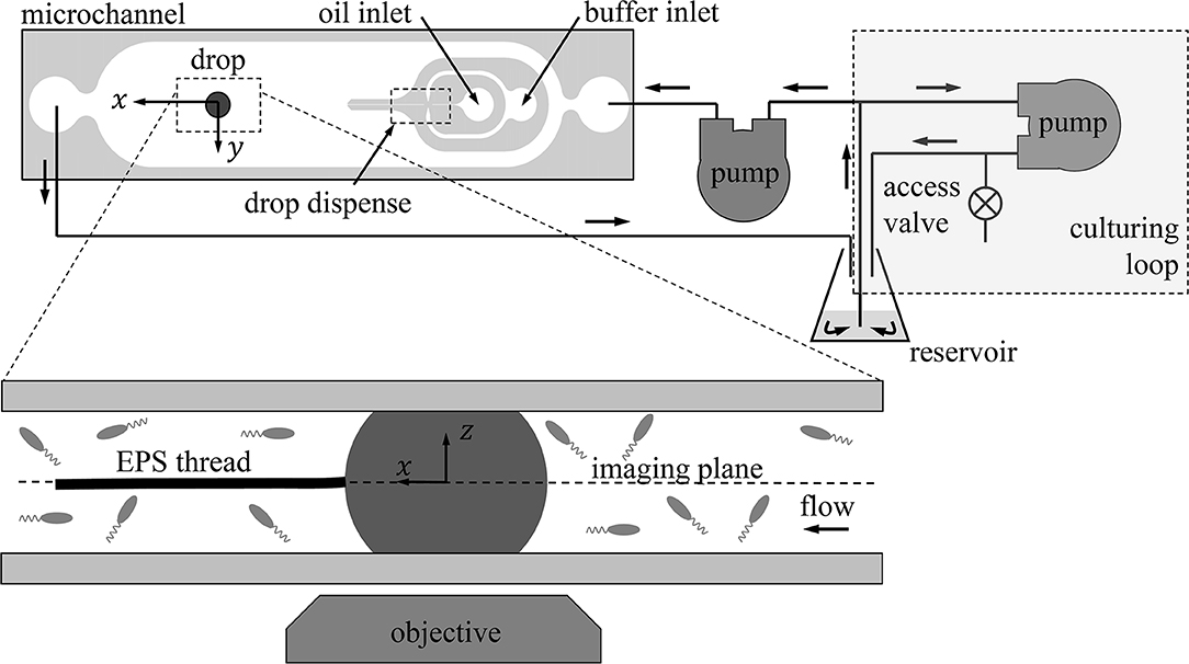
Figure 1. The experimental setup. At the top is the fluidics circuit consisting of the culturing loop (top right) where Pseudomonas sp. are cultured in situ and the observation loop that includes the microchannel (top left). The drop is generated in the flow focusing region indicated by “drop dispense.” The bulk of the bacteria suspension is contained in the reservoir (125 ml flask) during the experiment. A vertical cross section of the channel containing the pinned oil droplet is shown in detail at the bottom of the figure.

The flow circuit consisted of two loops as shown in Figure 1. Liquid drawn from the reservoir approached a T-junction, where liquid could either be rerouted back to the reservoir or sent toward the microfluidic channel for observation. When the peristaltic pump leading to the microfluidic channel (Figure 1) is off, this path is closed and the flow is restricted to the “culturing loop” (boxed-in region in Figure 1).

The microfluidic channel was fabricated using poly(dimethylsiloxane) (PDMS) (Dow Corning) (White et al., 2019) with a 10:1 ratio of PDMS and crosslinking agent. The PDMS channel and a clean glass microscope slide were exposed to air plasma (Harrick) for 1.5 min, and then the channel was bonded to the glass slide. The channel was then functionalized with a hydrophilic polyelectrolyte multilayer (PEM) deposited using a layer-by-layer technique (Bauer et al., 2010). Shortly after bonding, while the PDMS and glass were still plasma-activated, the channel was filled with 10 μM poly(allylamine hydrochloride) (PAH) (Sigma) in 0.1 M NaCl for 5 min. The channel was then rinsed with 0.5 M NaCl followed by filling with 10 μM poly(sodium 4-styrenesulfonate) (PSS) (Sigma) in 0.1 mM NaCl for 5 min. This procedure of alternating layers of PAH and PSS was continued until 4 PAH-PSS layers were formed. Additional details including a schematic of this process are found in (White et al., 2019). The channel was then rinsed with DI water and sterilized with 70% ethanol for the experiment.

A drop of oil (Macondo surrogate) was generated inside the microfluidic channel using a simple flow focusing junction (“drop dispense” in Figure 1). Oil was carefully introduced to the junction using a 1 ml glass syringe (Hamilton) and syringe pump (New Era Pump Systems) while a second syringe pump delivered sterile aqueous buffer to the junction to produce the drop. Once a drop was generated at this junction, the two syringe pumps were turned off and the drop traveled to the observation area of the channel shown in Figure 1 via flow generated by the peristaltic pump leading to the channel. Once in position, the peristaltic pump was also turned off such that the drop remained stationary. The diameter of the drop in this paper was 240 μm once in the observation area of the channel.

In tandem with setting up the experiment on the microscope, Pseudomonas sp. (ATCC 27259) (Vangnai and Klein, 1974) was cultured separately in 8 g/L nutrient broth on a rotary shaker at 120 rpm and room temperature. Pseudomonas sp. is an alkane degrader and also a motile bacterium. The culture was grown until saturation, which occurred after about 4 days and the optical density at 600 nm was OD₆₀₀>1. After the drop was generated as described above and the peristaltic pump leading to the channel was turned off, effectively closing off that loop, the system was inoculated via the access valve (Figure 1) with 100 μl of the Pseudomonas sp. culture grown outside of the system. The inoculated broth could then continuously recirculate in the culturing loop in Figure 1.

The system was left overnight which served three purposes. First, overnight the drop penetrated the PEM and became pinned, i.e., the contact area of the drop was fixed at both the PDMS and glass surfaces of the channel, but the oil-aqueous interface was freely mobile and the oleophobic contact angle between the drop and the channel walls was preserved. Second, by visually inspecting the microfluidic channel the next day, the sterility of the microfluidic channel was verified. Third, the Pseudomonas sp. in the culturing loop would grow to the target OD₆₀₀ = 0.4 desired for the experiment overnight.

After the culture reached the desired growth in the culturing loop, the peristaltic pump leading to the microchannel as shown in Figure 1 was turned on, allowing the culture to begin encountering the drop. The incoming velocity of the suspension in the microfluidic channel was 2.2 mm/s. A 20X S Plan Fluor ELWD objective (NA 0.45, depth of field ~5 μm) and differential interference contrast (DIC) imaging were used for imaging the drop with the inverted microscope. Images were recorded at 1,000 fps using a 1k ×1k CMOS high speed camera (IDT NR4) for 1 s periods spaced 10 min apart. The moment the first bacteria encountered the drop was considered t = 0, and thus high speed imaging sequences were taken at 10, 20, 30, etc. min after the first exposure to bacteria.

Flow Measurements

The high speed images are used to obtain flow measurements using micro-particle image velocimetry (μPIV)-assisted particle tracking velocimetry (PTV) (Evans et al., 2016) using the bacteria as flow tracers. Two quantities provide justification for using the bacteria as flow tracers. First, the Peclet numbers $P e = D_{d} D / | | \overset{⇀}{u} | |$ , where $| | \overset{⇀}{u} | |$ is the velocity magnitude and $D$ is the effective diffusivity of the bacteria including swimming, are Pe≫1, indicating that bacteria swimming does not significantly influence bacteria transport. Here $D = 2.26 \times 1 0^{- 9}$ m²/s with mean bacterial swimming speed of 22 μm/s (White et al., 2020). Second, the Stokes numbers $S t k = 2 / 9 (ρ_{b} / ρ_{f}) {(d_{b} / D_{d})}^{2} R e_{D}$ , where ρ_b and d_b are the bacteria density (~1.1 g/cm³) and characteristic size of the bacteria (~2 μm), are on the order of 10⁻⁵, indicating the bacteria will follow the streamlines. The measurement area was 720 × 720 pixels, and the depth of field (DOF) is ~5 μm so the flow measurements are averaged over this 5 μm thick slice of the flow. The DOF is approximated by $D O F = λ \sqrt{n^{2} - N A^{2}} / N A^{2}$ where λ is the light wavelength (~400–700 nm), n is the medium's index of refraction (~1.34), and NA is the numerical aperture (0.45) (Shillaber, 1944).

The microscope was focused in the center of the 100 μm thick channel. In a given imaging sequence captured at 1,000 fps for 1 s, every two consecutive images underwent a conventional cross-correlation PIV analysis (Roth and Katz, 2001). In a given image the bacteria locations are determined, and with the assistance of the PIV analysis their positions in the next image are found. Therefore, for each bacterium in each frame, a velocity vector is determined based on its position in the previous frame. Approximately 1,000 bacteria cells were identified per frame, providing about 1 × 10⁶ velocity vectors per high speed image period. The flow was averaged over the 1 s period and mapped onto a 4 pixel or 2.7 μm grid using a Taylor expansion scheme (Evans et al., 2016).

Conservation of Momentum

The pinned droplet has a diameter D_d and is subjected to a flow with incoming velocity U_f, density ρ_f and dynamic viscosity μ_f as shown in Figure 2A. The x-direction is in the positive flow direction. Assuming the flow is steady, the differential form of the balance of momentum is

\begin{array}{l} ρ_{f} (\overset{⇀}{u} \cdot \overset{⇀}{\nabla}) \overset{⇀}{u} = \overset{⇀}{\nabla} p + μ_{f} \overset{⇀}{\nabla} \cdot \overset{⇀}{\nabla} \overset{⇀}{u} & (1) \end{array}

where $\overset{⇀}{u}$ is flow velocity vector, $\overset{⇀}{\nabla}$ is the gradient operator, and p = P−ρ_fgh is a modified pressure (hereafter called simply pressure) i.e., static (P) minus hydrostatic (ρ_fgh) pressure where g is gravitational acceleration and h is depth. For analysis, the velocities are scaled by U_f, the lengths are scaled by D_d, and pressure is scaled by μ_fU_f/D_d. Using this scaling, the x- and y-component, respectively, of the differential form of the momentum balance is

\begin{array}{l} R e_{D} (u_{x}^{*} \frac{\partial u_{x}^{*}}{\partial x^{*}} + u_{y}^{*} \frac{\partial u_{x}^{*}}{\partial y^{*}}) = - \frac{\partial p^{*}}{\partial x^{*}} + (\frac{\partial^{2} u_{x}^{*}}{\partial {x^{*}}^{2}} + \frac{\partial^{2} u_{x}^{*}}{\partial {y^{*}}^{2}}), \\ R e_{D} (u_{x}^{*} \frac{\partial u_{y}^{*}}{\partial x^{*}} + u_{y}^{*} \frac{\partial u_{y}^{*}}{\partial y^{*}}) = - \frac{\partial p^{*}}{\partial y^{*}} + (\frac{\partial^{2} u_{y}^{*}}{\partial {x^{*}}^{2}} + \frac{\partial^{2} u_{y}^{*}}{\partial {y^{*}}^{2}}) & (2) \end{array}

where $u_{x}^{*}$ and $u_{y}^{*}$ are the x- and y-components of the velocity, and Re_D = ρ_fU_fD_d/μ_f is the Reynolds number. The superscript “^*” indicates a non-dimensionalized parameter. In both rows, the left-hand side contains the advection terms, and on the right-hand side is the pressure gradient followed by the viscous stresses. Using flow measurements from the previous section to obtain $u_{x}^{*}$ and $u_{y}^{*}$ , each term in both rows of Eq. (2) can be determined directly, including the x- and y-components of the pressure gradient. The derivatives of u^* and v^* are calculated using second order central or forward/backward finite differences. The pressure gradient, if properly integrated, can yield the pressure p, which we will see in the Results section is a crucial part of the force balance on the droplet. In the next section, we describe how the drag force on the drop is estimated.

FIGURE 2

Figure 2. (A) shows a schematic depicting the stationary drop (gray circle) with diameter D_d, density ρ_f and dynamic viscosity μ_d, subjected to a flow with upstream velocity U_f, density ρ_f, and dynamic viscosity μ_f. In (B) a control region ABCD is drawn around the drop where the positive x-direction is in the flow direction.

Control Volume Analysis

A control volume analysis is used to estimate the drag force on the pinned droplet. In this analysis, the droplet pinned between the two walls of the microfluidic channel is assumed to be a cylinder in a 2D flow. A control region ABCD as shown in Figure 2B is drawn around the droplet, and the control volume is taken as the area between the ABCD box and the droplet surface extending infinitely into and out of the page. The unit normal vector n points outside the control volume as shown in Figure 2B. With this geometry in mind, the integral form of the x-momentum balance is

\begin{array}{l} \int_{A B C D} [R e_{D} (\overset{⇀}{n} \cdot {\overset{⇀}{u}}^{*}) u_{x}^{*} + n_{x} p^{*} - \overset{⇀}{n} \cdot \overset{⇀}{\overset{⇀}{τ}} \cdot {\overset{⇀}{e}}_{x}] d S^{*} \\ + F_{d}^{*} = 0, & (3) \end{array}

where $F_{d}^{*} = F_{d} / μ U_{f}$ is the dimensionless drag force per length or viscous drag coefficient, ${\overset{⇀}{\overset{⇀}{τ}}}^{*} = {\overset{⇀}{\nabla}}^{*} {\overset{⇀}{u}}^{*} + {({\overset{⇀}{\nabla}}^{*} {\overset{⇀}{u}}^{*})}^{T}$ is the dimensionless stress tensor, and S^* is the perimeter ABCD. Evaluating each term in Eq. (3) besides $F_{d}^{*}$ yields the following form:

\begin{array}{l} F_{d}^{*} = \int_{A, C} [R e_{D} (u_{x, A}^{* 2} - u_{x, C}^{* 2}) + (p_{A}^{*} - p_{C}^{*}) - (τ_{x x, A}^{*} - τ_{x x, C}^{*})] d y^{*} \\ + \dots \int_{B, D} [R e_{D} (u_{y, D}^{*} u_{x, D}^{*} - u_{y, B}^{*} u_{x, B}^{*}) - (τ_{y x, D}^{*} - τ_{y x, B}^{*})] d x^{*} . & (4) \end{array}

In Eq. (4), the stresses are defined in terms of the x- and y-components of velocity as $τ_{x x}^{*} = 2 \partial u_{x}^{*} / \partial x^{*}$ and $τ_{y x}^{*} = \partial u_{x}^{*} / \partial y^{*} + \partial u_{y}^{*} / \partial x^{*}$ . The subscripts A, B, C, and D indicate velocity, pressure or stress profiles over those respective boundaries. Thus, each term can be evaluated using the experimental flow measurements directly except for $p_{A}^{*}$ and $p_{C}^{*}$ .

Since the pressure gradients are known using Eq. (2), these gradients can be integrated over the region ABCD to estimate the pressure over boundaries A and B. Integration is performed using first order forward/backward finite differences. Beginning at a corner of the control volume, the pressure gradient field is integrated both clockwise and counterclockwise over ABCD. The resulting pressure profiles for both integration directions are averaged to produce $p_{A}^{*}$ and $p_{C}^{*}$ . Combined with the flow measurements $u_{x}^{*}$ and $u_{y}^{*}$ , and calculated $τ_{x y}^{*}$ and $τ_{x x}^{*}$ , the drag force per length $F_{d}^{*}$ is calculated.

Results and Discussion

EPS Aggregations and the Hydrodynamic Impacts

In Figure 3 the measured flow field around the stationary droplet prior to any bacterial attachment (20 min after first bacterial encounter) is presented as a series of contour plots. Figure 3A shows the u^* and v^* components of the velocity field. Due to the symmetry of the flow field, we plot v^* on the left half and u^* on the right half of Figure 3A separated by the vertical black line through y^* = 0. Similarly, the viscous shear ( $τ_{x y}^{*}$ ) and normal ( $τ_{x x}^{*}$ ) stresses are shown in Figure 3B, and the two components of the pressure gradient ∂p^*/∂y^* and ∂p^*/∂x^* are shown in Figure 3C. The pressure gradient fields are calculated using Eq. (2). The flow field shown in Figure 3 is expected of Stokes flow (Re_D < 0.5), which has symmetry both left and right as well as top to bottom in the streamwise direction.

FIGURE 3

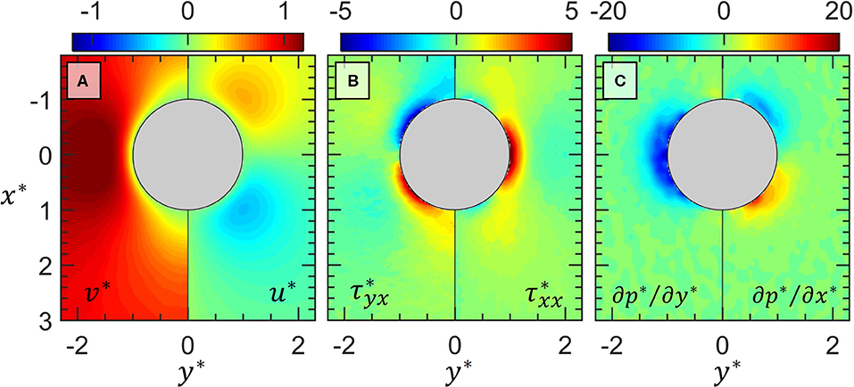
Figure 3. The measured flow field around the oil drop (gray circle) prior to attachment of any bacteria. In (A) the y-component (left half) and x-component (right half) of velocity is shown. In (B) the shear (left half) and normal (right half) viscous stresses are shown. In (C) the y-component (left half) and x-component of the pressure gradients are shown. All quantities are normalized as described in the text. The magnitudes correspond to the respective color bar above each plot.

At first glance, raw images from a high speed image sequence captured 50 min after the first bacterial encounter (Figure 4) do not appear to show any obvious aggregates or presence of EPS filaments. A video of the sequence of images shown in Figure 4 is available in the (Video S1). In Figure 4A, a cropped image 44 ms into the 1 s imaging period appears to show only single distributed bacteria freely flowing past the drop (dark semi-circle in Figure 4), or in some cases clusters of 2-3 bacteria can be identified. In Figure 4A we have pointed out one particular cluster of ~3 bacteria (red arrow). A dotted black line is plotted on top of the image representing a streamline passing through this cluster at this instant in Figure 4A. This streamline is determined from the measured mean flow field over the entire 1 s imaging period. In Figure 4B, 100 ms later, the same cluster is spotted in a new position along the same streamline as expected.

FIGURE 4

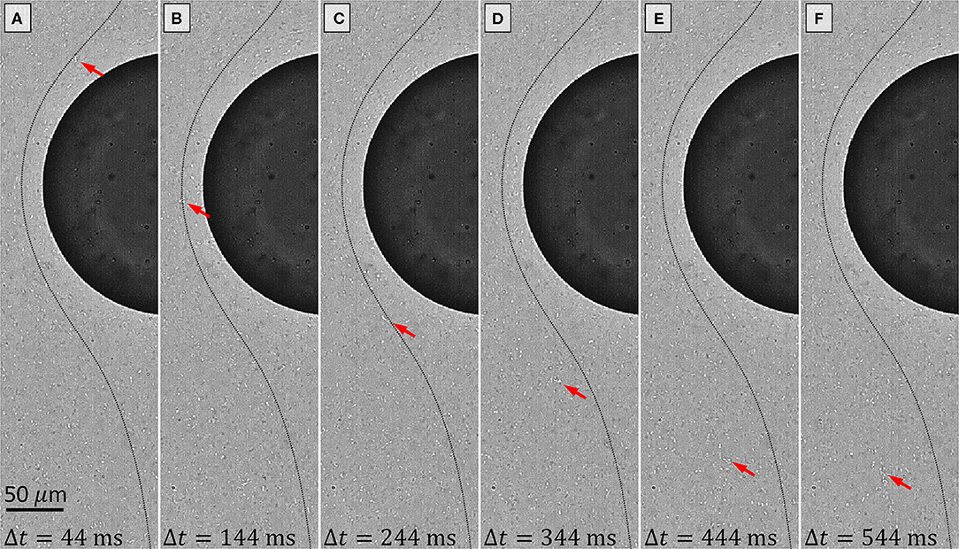
Figure 4. Raw images of a high speed imaging sequence captured 50 min after the first bacteria encounter are shown. The time step for each image during the 1 s imaging sequence is shown at the bottom, and 100 ms separates each image. A video of this sequence is provided in the Video S1. In (A) a cluster of ~3 bacteria is indicated by the red arrow. The thin dotted black line is a streamline of the mean flow passing through the current position of the indicated cluster. In (B) the cluster has traveled along the streamline. In (C) the cluster encounters a transparent EPS filament (confirmed in Video S1). In (D–F) the cluster has now deviated from the streamline and is trapped in the EPS filament.

However, in Figure 4C, the cluster appears to run into an invisible obstacle, which is confirmed by viewing Video S1. As other bacteria seem to flow past freely, this cluster stalls for a moment, and 100 ms later the cluster drifts away from its streamline in Figure 4D. In fact, this cluster has encountered an EPS filament, anchored on the drop surface. Since the depth of field in these images is ~5 μm, and bacteria (1–3 μm) seemingly flow past the same location as the trapped cluster without getting trapped themselves, this suggests the EPS thread is quite thin and localized, perhaps being in the vicinity of 1 μm in diameter or smaller. We stress that we do not directly measure the filament diameter, but rather infer its diameter based on the DOF and the observation that not all bacteria within this DOF encounter the filament. Furthermore, we note that in subsequent drag calculations, the filament diameter is not included in the control volume analysis and has no direct impact on our calculations.

In Figure 4E, the same cluster has traveled along the EPS filament a little further downstream. It is unclear if the bacteria cluster is moving through the EPS material in the filament, or if the EPS material itself is moving or deforming, or if both could be happening simultaneously. Another 100 ms later in Figure 4F, the bacteria cluster has remained in approximately the same location. In the latter half of this imaging sequence (Video S1), the bacterial cluster can be seen traveling further downstream and out of frame.

Figure 4 highlights two important things. First, these early EPS filaments and the attached bacteria are quite transient, with EPS filaments forming and detaching, and bacteria attaching and subsequently moving downstream along the filament. Second, this demonstrates that preformed EPS threads without attached bacteria and attached to a liquid drop are capable of capturing bacteria as they pass by, and in this case this appears to be the primary mode of aggregation in comparison to the mode that bacteria attached to the drop transfer to the EPS filament (Das and Kumar, 2014). The origins of the preformed EPS threads are more difficult to determine. In one scenario, it is plausible that bacteria that are attached to the drop surface are responsible for secreting EPS that is extruded downstream due to flow shear similar to observations by other researchers (Marty et al., 2012; Valiei et al., 2012; Das and Kumar, 2014; Scheidweiler et al., 2019).

The consequences of these apparently short-lived EPS threads and their attached bacteria are twofold. First, the trapped bacteria effectively “hitch a ride” on the tails of the droplet, affecting the transport of the bacteria. In the water column, one can imagine bacteria stowing away on a rising oil droplet, traveling many meters or perhaps kilometers away from its origin. This would have major implications on marine ecology, influencing microbial distribution and the food web in the water column (Kiørboe et al., 2002). Second, the EPS filament and attached bacteria manipulate the flow around the drop. Figure 5 depicts the mean flow field around the drop 50 min after first bacterial encounter, the same imaging period shown in Figure 4. In Figures 5A,D, the v^*and u^* fields are clearly disturbed by the presence of EPS filaments present behind the drop. The presence of these threads is even more apparent in the $τ_{x y}^{*}$ and $τ_{x x}^{*}$ (Figures 5B,E), and ∂p^*/∂y^* and ∂p^*/∂x^* (Figures 5C,F) fields. In fact, the ∂p^*/∂x^* field seems to be particularly capable of indicating the positions of otherwise invisible EPS filaments and attached bacteria. In Figure 5F, ~4 distinct EPS threads are distinguished by the steep increase in the pressure gradient. The filament on which the bacteria cluster in Figure 4 become trapped has the most pronounced signal on the left trailing side of the drop. It is important to note that we are presenting the mean flow field here, and it is apparent in Figure 4 that attached bacteria and bacteria clusters are not necessarily stationary even over the 1 s imaging period.

FIGURE 5

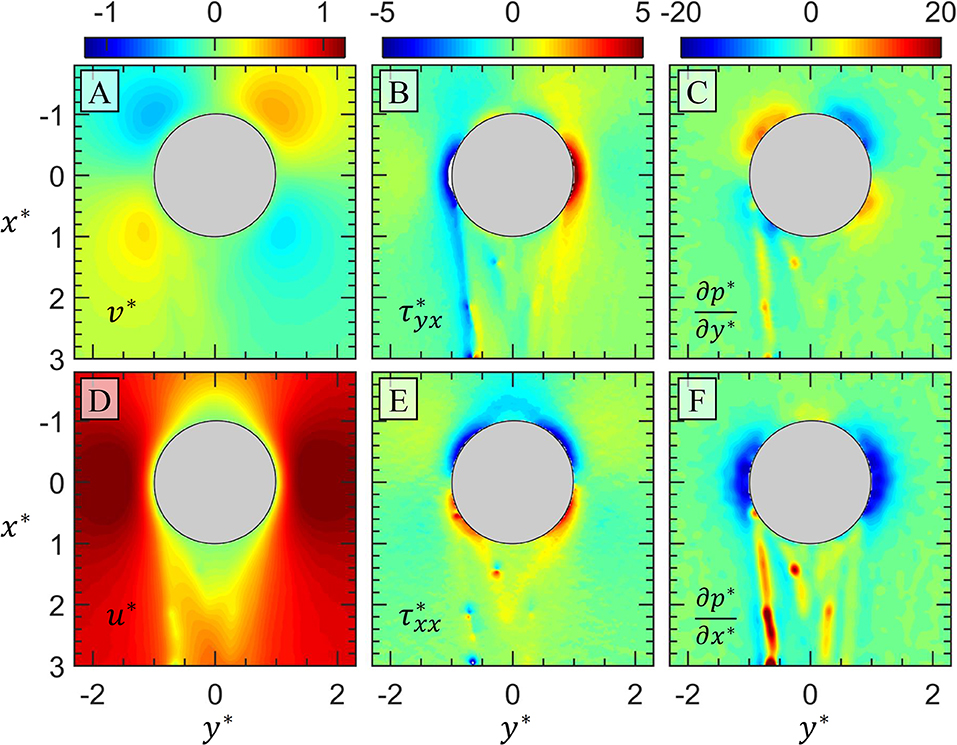
Figure 5. The measured flow field around the oil drop (gray circle) after bacterial streamers have developed on the trailing half of the drop 50 min after the first bacteria encounter (Figure 4). In (A) the y-component and (D) x-component of velocity is shown. In (B) the shear and (E) normal viscous stresses are shown. In (C) the y-component and (F) x-component of the pressure gradients are shown. All quantities are normalized as described in the text. The magnitudes correspond to the respective color bar above each column of plots.

It is reasonable to wonder if the disrupted flow around the drop in Figure 5, and the apparently reduced velocity behind the drop shown in Figures 5A,D compared to the same drop without attached bacteria (Figure 3), could enhance bacteria transport to the drop surface due to bacteria motility. That is, will the mobile bacteria swim fast enough relative to the decreased flow that attachment is increased in Figures 4, 5 vs. Figure 3? To answer this question, we plot the Peclet numbers, $P e = D_{d} D / | | \overset{⇀}{u} | |$ , where $| | \overset{⇀}{u} | |$ is the velocity magnitude and $D$ is the effective diffusivity of the bacteria including swimming. We estimate $D$ to be 2.26 × 10⁻⁹ m²/s by separately tracking bacteria trajectories in quiescent medium [Supplemental Materials of (White et al., 2020)]. Contours of Pe(x^*, y^*) when no attached bacteria are present (Figure 3) are plotted in Figure 6A. Pe is largely greater than one aside from very close to the drop surface. In Figure 6B, Pe(x^*, y^*) is plotted at the instant 50 min after the first bacterial encounter (Figures 4, 5). The Peclet numbers are reduced directly behind the drop in Figure 6B (larger green region on the trailing side of the drop) which is a direct consequence of the reduced velocity (Figures 5A,D). This lowering of the Pe is highlighted in Figure 6C where Pe from Figures 6A,B along y^* = 0 are plotted. Still, Peclet numbers are largely Pe > 1, and thus flow advection is the dominant transport mechanism for the bacteria and swimming is not expected to have a significant effect on bacteria transport outside of 1-2 bacteria lengths away from the drop surface. Additionally, this provides justification for the use of the suspended bacteria as flow tracers for the purposes of flow measurements (in addition to the low Stokes numbers as described in the Materials and Methods).

FIGURE 6

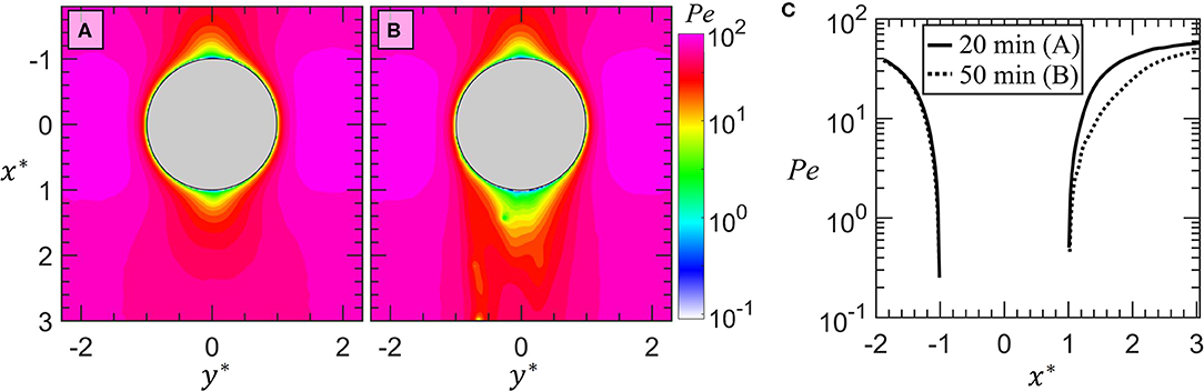
Figure 6. In (A), Peclet numbers are shown for the drop prior to attachment of bacteria at the same instance depicted in Figure 3. In (B), Peclet numbers are shown for the same drop after bacterial streams have developed on the trailing half of the drop at the same instance depicted in Figure 5. The color contours are on a log scale with magnitudes corresponding to the color bar. In (C) a semilog plot of the Peclet numbers along y^* = 0 (i.e. through the center of the drop) is shown without attached bacteria (A at 20 min) and with streamers (B at 50 min).

Returning to the hydrodynamic impacts of an EPS filament, we plot the ∂p^*/∂x^* field with streamlines overlaid (black lines) for 50 min after first bacterial encounter (Figure 7A) and 70 min after first bacteria encounter (Figure 7B). The ∂p^*/∂x^* field is plotted due to its ability to highlight the presence of the invisible EPS filaments. In Figure 7A, the EPS filament discussed in Figure 4 is indicated by the red arrow. It is clear from this plot that the streamlines cross the EPS filaments, a result that is necessary due to the elastic nature of the filaments (Autrusson et al., 2011). This will have significant hydrodynamic consequences. In Figure 7B, after 20 min have elapsed since Figure 7A, the EPS filament indicated in Figure 7A has disappeared while two remain in similar positions as two EPS filaments in Figure 7A. Now in Figure 7C, the streamlines from Figure 7B (black lines) are plotted on top of the streamlines from Figure 7A (red lines) to highlight the differences between them. Specifically, on the left half of the downstream side of the drop, it is clear that the presence of the indicated filament in Figure 7A “pushed” the streamlines in the negative y-direction. This demonstrates that a single EPS filament can cause a significant deviation in the streamlines. This widening of the streamlines due to the presence of an EPS filament effectively increases the hydrodynamic profile of the drop, which indicates an increase in “form drag” (in contrast to drag due to increased friction).

FIGURE 7

Figure 7. In (A) contours of ∂p*/∂x* for the drop at 50 min (Figure 5F) is plotted with streamlines overlaid. In (B) contours of ∂p*/∂x* around the same drop at 70 min is shown with streamlines overlaid and originating at the same x-coordinates as (A). A streamer indicated by the red arrow in (A) has detached in (B). In (C) the streamlines from (B) (black lines) are plotted on top of the streamlines from (A) (red lines) to show the deviation in streamlines caused by the streamer indicated by the red arrow in (A).

The ultimate hydrodynamic impact of these attached EPS filaments is elucidated though an analysis of the momentum balance in the system using Eq. (4). Here, the drag force is the addition of the contribution of five terms: the x-momentum difference across surfaces A and C, $R e_{D} (u_{x, A}^{* 2} - u_{x, C}^{* 2})$ ; the x-momentum difference across surfaces D and B, $R e_{D} (u_{y, D}^{*} u_{x, D}^{*} - u_{y, B}^{*} u_{x, B}^{*})$ ; the pressure difference across surfaces A and C, $(p_{A}^{*} - p_{C}^{*})$ ; the viscous normal stress difference across surfaces C and A, $(τ_{x x, C}^{*} - τ_{x x, A}^{*})$ ; and the viscous shear stress difference across surfaces B and D, $(τ_{y x, D}^{*} - τ_{y x, B}^{*})$ . Note the negative signs in front of the viscous terms in Eq. (4) have been distributed here. We designate each of these terms as pieces of the total momentum budget, and by analyzing these five contributions we can further analyze how the presence of these EPS threads and attached bacteria are impacting the hydrodynamics.

Figures 8B–F plots these five terms from Eq. (4) for the drop 20, 50, and 70 min after the first bacterial encounter. The area under the curve of each plot adds up to the total drag force on the drop (note that we plot $(τ_{y x, D}^{*} - τ_{y x, B}^{*})$ and $(τ_{x x, C}^{*} - τ_{x x, A}^{*})$ , i.e., the negative signs in front of the viscous terms in Eq. (4) have been distributed through those terms). In Figures 8B,C, we see minimal differences when comparing the drop without attached aggregates (20 min) and with attached aggregates (50 and 70 min). In Figure 8E, we see clear differences between the three snapshots of the drop. The curve taken at 50 min after the first bacterial encounter has a pronounced peak at x^* = −0.3 caused by the EPS filament indicated in Figure 7A as well as the smaller filament to its right. Another smaller peak at x^* = 0.25 is caused by the EPS filament on the right side of the drop in Figure 7A. At 70 min, and the two EPS filaments identifiable in Figure 7B cause similar sized peaks in Figure 8E. However, it is important to take note of the magnitude of the vertical axis in Figure 8E; the $R e_{D} (u_{x, A}^{* 2} - u_{x, C}^{* 2})$ does not contribute as much to the drag as the viscous stresses, $τ_{x x}^{*}$ (Figure 8F) and $τ_{x y}^{*}$ (Figure 8C), and the pressure p^* (Figure 8D). The magnitudes of these terms are an order of magnitude greater than the other two terms. Furthermore, the pressure difference in Figure 8D is the term most significantly affected by the presence of the EPS filaments.

FIGURE 8

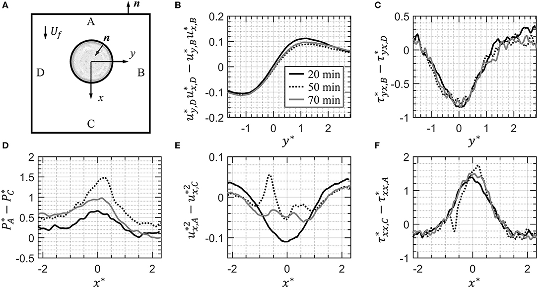
Figure 8. In (A) the control region ABCD is shown again for convenience. In (B–F) the terms from Eq. (4) contributing to the drag force on the drop are plotted for the drop prior to attached bacteria (20 min, Figure 3), after attachment of several streamers on the trailing half of the drop (50 min, Figure 5), and after one streamer present at 50 min has detached (70 min, Figure 7B). The area under the curve in each plot is added together to determine the drag at each instant in time according to Eq. (4).

In Table 1, the magnitudes of the individual terms in Eq. (4) (i.e., area under the curves in Figure 8) are tabulated for the drop 20 min after the first bacterial encounter (i.e., no attached EPS filaments or aggregates), 50 min after the first exposure (i.e., with several EPS filaments), and 70 min (i.e., one less filament than at 50 min as shown in Figure 7). As seen graphically in Figure 8, this table shows that the pressure term is the most affected by the presence of the EPS filaments, more than doubling from 20 to 50 min, and then decreasing some at 70 min after the filament highlighted in Figure 7 has detached. This is corroborated by the observation of the EPS filaments significantly deviating the streamlines, and indication of the hydrodynamic profile of the drop becoming larger. As a result, the drag increase is due to “form drag” as mentioned earlier, i.e., the drag is increased primarily due to the modulation of the pressure field around the drop.

TABLE 1

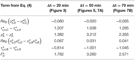
Table 1. Magnitudes of terms in the momentum balance Eq. (4) and the viscous drag coefficients $F_{d}^{*}$ for the drop 20, 50, and 70 min after the first encounter with bacteria.

The sum of each term gives the viscous drag coefficient $F_{d}^{*}$ shown in the bottom row of Table 1 which allows us to quantify the impact of the EPS filaments and attached bacteria on the drag force experienced by the drop. The drag coefficient increases by 85% from the instant at 20 min (no filaments) to 50 min (several filaments). In Figure 7C, we showed that the detachment of a single EPS filament produced a noticeable deviation in the streamlines, and this resulted in a 27% reduction in the drag coefficient from 50 min (Figure 7A) to 70 min (Figure 7B). However, the drag coefficient at 70 min is still 46% greater than the drag coefficient for the clean drop at 20 min.

It should be noted here that the EPS filaments extend outside the image frame, and so the full effect of the filaments on the flow field and the drag cannot be realized. In fact, this suggests that the drag measurements reported here are likely conservative, and if the entire manipulated flow field were captured the apparent drag increase may be increased further. Furthermore, we have only to this point captured these flow fields in the early stages of the EPS filament generation. On the one hand, this importantly shows that the EPS filaments, and as a consequence the drag coefficients, are rather transient in the early period of initial bacteria attachment to the drop. However, in (White et al., 2019) we showed that bacteria can form quite robust aggregates and streamers on an oil drop by three bacterial isolates and six natural assemblages using ecology-on-a-chip microcosm platform, and it is reasonable to expect drastic increases in drag when these larger aggregates develop.

Deviations From the DWH Environment

It is clear that these EPS filaments and their attached bacteria can have a significant impact on the drag of the drop, and ultimately we are interested in knowing how this will impact the transport and fate of the oil droplet in the water column after encountering a microbial bloom, and also how this may in turn affect the microbial community. However, we must stress that caution be taken when interpreting the results in the context of the DWH spill. These laboratory experiments have several deviations from the real environment during the DWH oil spill:

1) We use a bacterial isolate [Psuedomonas sp. (ATCC 27259)], albeit an alkane degrader isolated from a marine environment (Vangnai and Klein, 1974). A community of bacteria, and in particular a community representative of the initial deep sea plume including Oceanospirillales, Colwellia, and Cycloclasticus (Hazen et al., 2010; Mason et al., 2012) would provide more relevant results in future work;

2) The aqueous phase contains ample nutrients and these nutrients are not presentative of those leading to the microbial bloom in the DWH deep sea plume;

3) The cell density is estimated to be ~10⁸ cells/ml, which is quite high but allows us to produce high resolution flow measurements. In the deep sea plume, reported cell densities were as high as 1,540,000 cells/ml (Kleindienst et al., 2016), and in localized areas they were perhaps more dense.

4) The measurements were made at room temperature and pressure;

5) The drop is not a sphere but rather more of a disc with 100 μm thickness, 240 μm diameter, and a curved edge with an oleophobic contact angle with the microchannel top and bottom walls.

Therefore, it is important to consider the results presented here in the context of these caveats. For example, in the real environment, time scales for developing bacterial aggregates, as well as the morphology and ultimate hydrodynamic impacts of the aggregates, could be quite different. Nonetheless, we have demonstrated a very important mechanism and its plausible impacts on the drag of a rising oil droplet through a dense microbial bloom that has seldom been considered when predicting the fate of submillimeter oil droplets during the DWH spill. Incorporating these bacteria-mediated EPS filaments, which can grow into large aggregates, into oil droplet transport models could drastically affect our understanding of the distribution and fate of these oil droplets and their impact on the microbial community.

Conclusions

In this paper we used an ecology-on-a-chip platform (White et al., 2019) to demonstrate the significant hydrodynamic impacts that nearly invisible EPS threads can have on an emulated droplet rising through a bacterial suspension. Instead of observing a droplet rising through the suspension, we have flowed a bacterial suspension past a pinned droplet while periodically recording high speed images used for flow measurements. These threads were observable only by either identifying bacteria and bacteria clusters trapped in the threads (Figure 4) or by using anomalies in the flow measurements (Figure 5). In fact, we observed a bacteria cluster, which initially follows a mean flow streamline, become captured by an EPS thread (Video S1).

These EPS threads have two major consequences. First, the bacteria can hitch a ride on these threads and significantly alter their transport in the water column. Although the threads are initially transient and detach frequently in the time period over which we made our measurements, over time a more stable and robust aggregate or streamer can form (White et al., 2019), allowing the bacterial stowaways to travel much greater distances, potentially greatly affecting their distribution in the water column. Second, these threads immediately and significantly perturb the flow field around the drop, affecting the hydrodynamics and drag experienced by the drop.

By performing a control volume analysis around the drop, the conservation of momentum provided more insight into how the EPS threads affected the drag. Specifically, it was found that modulations in the pressure field were the primary contributor to increasing drag on the drop (Table 1), caused by the threads widening the streamlines (Figure 7C). These threads, though estimated to be about 1 μm thick or smaller, appear to be effective at deviating the streamlines. Comparing a clean drop without any EPS threads or attached bacteria to the same drop after about four EPS threads appear to be attached, the viscous drag coefficient increased by 85%. To demonstrate the impact of a single EPS thread, when one thread had detached from the drop (Figures 7A,B), the drag coefficient decreased by 27%.

There are several caveats to keep in mind when considering these results in the context of the real open ocean as described in the Results and Discussion: the bacteria community, the aqueous phase composition, the temperature and pressure, and the shape of the drop are not the same as the real conditions. However, it is plausible to expect similar EPS threads and bacterial aggregates to form on a real drop rising through a microbial bloom in the water column, and hydrodynamic impacts would be analogous to those quantified in these microfluidic experiments.

With this in mind, we can put an 85% drag coefficient increase on a spherical drop in perspective. Assuming Stokes flow (Re_D < 0.5), the rising velocity of a spherical droplet is inversely proportional to the drag coefficient (i.e., C_d = 24/Re_D). Therefore, an 85% increase in the drag coefficient corresponds to a 46% reduction in the rising velocity. We can alternatively put an 85% drag increase in the perspective of biodegradation, where it is common in modeling studies to assume the drop volume decreases with time according to available biodegradation half-life data (North et al., 2015). Since the drop diameter is also inversely proportional to the drag coefficient, to achieve an 85% increase in the drag coefficient would require a 46% reduction in the drop diameter, or about a 10% reduction in the drop volume. Thus, the hydrodynamic impact of several EPS threads (Figure 5) attached to a rising droplet is roughly on the same order of magnitude as a 10% reduction in the drop's volume.

While more work needs to be done with more ecologically relevant conditions (bacteria, temperature, and pressure, aqueous phase), the mechanism investigated in this paper and the measurable impacts on the hydrodynamics and the drag experienced by the drop are significant and will drastically affect drop transport and fate predicted by current modeling efforts.

Data Availability Statement

Data are publicly available through the Gulf of Mexico Research Initiative Information & Data Cooperative (GRIIDC) at https://data.gulfresearchinitiative.org (doi: 10.7266/N7N58JTF, doi: 10.7266/N7BV7F6V).

Author Contributions

AW and JS designed research and analyzed data. AW, MJ, and JS performed research. AW and MJ contributed new tools. All authors wrote the paper.

Funding

This research was partially supported by the grants from the Gulf of Mexico Research Initiative (GoMRI) SA18-17/UTA17-001449 and SA15-19/UTA16-000545 and a grant from ExxonMobile under grant no. A4006200. Microfabrication equipment is partially supported from ONR under grant no. W911NF-17-1-0371.

Conflict of Interest

The authors declare that the research was conducted in the absence of any commercial or financial relationships that could be construed as a potential conflict of interest.

Supplementary Material

The Supplementary Material for this article can be found online at: https://www.frontiersin.org/articles/10.3389/fmars.2020.00294/full#supplementary-material

Video S1. A 700 ms segment of the high speed image sequence captured 50 min after the first bacterial encounter is shown. The playback is at 1/100 real speed. The oil drop (black half circle) has a radius of 120 μm. White dots in the video are suspended bacteria. Initially a cluster of ~3 bacteria are circled in red. A black dotted line represents the mean flow streamline passing through this bacteria cluster in the initial frame. As the video plays, the cluster can be seen following the streamline until suddenly encountering an EPS thread on the trailing side of the drop. The cluster then deviates from the streamline, following the path of the EPS thread. The bacteria become momentarily trapped in the thread, and toward the end of the clip they again begin to drift downstream along the thread out of the frame.

References

Alldredge, A. L., and Silver, M. W. (1988). Characteristics, dynamics, and significance of marine snow. Prog. Oceanogr. 20, 41–82. doi: 10.1016/0079-6611(88)90053-5

ORIGINAL RESEARCH article

Hydrodynamics of a Rising Oil Droplet With Bacterial Extracellular Polymeric Substance (EPS) Streamers Using a Microfluidic Microcosm

Introduction

Materials and Methods

Experiment Setup and Procedure

Flow Measurements

Conservation of Momentum

Control Volume Analysis

Results and Discussion

EPS Aggregations and the Hydrodynamic Impacts

Deviations From the DWH Environment

Conclusions

Data Availability Statement

Author Contributions

Funding

Conflict of Interest

Supplementary Material

References

This article is part of the Research Topic

People also looked at