Estimating Nitrogen Runoff From Agriculture to Coastal Zones by a Rapid GIS and Remote Sensing-Based Method for a Case Study From the Irrigation District Río Mayo, Gulf of California, México

Introduction

Increased nutrient concentrations due to fertilizer runoff from agricultural areas is one of the main ecological problems for costal zones (Páez-Osuna et al., 2017). The increase in nutrients has had multiple consequences on marine ecosystems, such as harmful algal blooms, zones of hypoxia or anoxia, and loss of biodiversity (Breitburg et al., 2018). This is a global problem that has been documented for various seas, including the Baltic Sea, the China Sea coast, as well as the Mississippi delta and its influence on the Gulf of Mexico (Raymond et al., 2012; Breitburg et al., 2018).

Estimating fertilizer runoff from agricultural areas is usually a complex exercise, since it involves a large number of sampling sites distributed over a large area with different terrain characteristics, which can range from inaccessible mountainous areas to coastal plains (He and DeMarchi, 2014; Hofmeister et al., 2016; López-Vicente et al., 2016). As a result, certain areas are left unsampled. In addition, the temporality of planting, that is, the agricultural cycles and, in some cases, the modification of the hydrological basin by new channels and drains (Rhoads et al., 2016), should also be taken into account. Nevertheless, estimating the runoff of agricultural compounds toward both continental and marine bodies of water is essential to understand their potential effects (Davidson et al., 2014; Breitburg et al., 2018).

Some research has shown the advantages of remote sensing (RS) and Geographic Information Systems (GIS) to estimate nitrogen input in the coastal zones. Sun et al. (2016) used GIS to upscale and visualize total nitrogen runoff losses from field to regional scales. They also characterized significant spatiotemporal variation characteristics during rice seasons, which were positively related to fertilizing rates and precipitation. Mouri et al. (2010) used Landsat images and multivariate analysis to survey the load of total nitrogen in stream water in the Nagara River Basin. Chang (2008) showed the capacities of GIS analysis to study processes that occurred in the past. He examined spatial patterns of eight parameters of water quality – including total nitrogen – in the period 1993–2002 and concluded that spatial analysis of watershed data at different scales is useful in identifying the fundamental spatiotemporal distribution of water quality. In a more recent work, Mainali and Chang (2018) analyzed the seasonal trends of water quality parameters, including total nitrogen, in the Han River Basin (HRB) of South Korea using the Mann–Kendall test. They explored the effects of anthropogenic (land cover and population) and natural (topography and soil) factors using Moran’s Eigenvector-based spatial filtering regressions at four different spatial scales. All these examples show advantages of using GIS and RS to estimate nitrogen input coming from agricultural and urban areas in particular water bodies.

In the northwestern area of the Gulf of California, there is extensive use of chemicals in fertilizer, particularly nitrogen based. Studies show that the observed average of 250 kg/ha, although recommended by both agricultural organizations and the Instituto Nacional de Investigaciones Forestales (SAGARPA, 2015), are actually excessive (Beman et al., 2005; Harrison et al., 2005; Christensen et al., 2006; Armenta-Bojórquez et al., 2012). Therefore, it can be safely assumed that large amounts of fertilizers are swept toward the coastal zones, increasing the input of nutrients.

Sonora is one of the main agricultural and fishing states in Mexico, distinguished for both its coastline on the Gulf of California as well as its mountainous areas. Sonora is one of the main states within Mexico facing the problem of agricultural runoff. It is among the top producers of grains and vegetables, grown mostly in the coastal valleys. The valleys have an extensive network of drainage canals for irrigation and wells for groundwater extraction in districts like Río Mayo, El Yaqui, or Guaymas (Pedroza-González and Hinojosa-Cuéllar, 2014). The runoff flows directly into the Gulf of California and its beaches.

While it has been estimated that the agricultural areas of Sonora and Sinaloa only contribute with (∼0.6% of the nitrogen input to the Gulf of California (Páez-Osuna et al., 2017), it also has been reported that this effect can occur at local and medium scale and that these agricultural areas are one of the main vectors of pollution (pesticides, fertilizers, etc.) of the marine systems surrounding the Gulf of California (Beman et al., 2005; Montes et al., 2012).

The objective of our research was to study the amount of agricultural nitrogen fertilizer entering the coastal ecosystem of the Gulf of California. For this purpose, we used the agricultural parcels as a study case in the irrigation district of Río Mayo (Sonora estate, Mexico) to generate a rapid GIS and remote sensing-based methodology.

Materials and Methods

Study Zone

The irrigation district of Río Mayo is located in the southern part of Sonora (Figure 1). It has an average annual precipitation of 388 mm and an average annual temperature of 21.4°C (Pulido Madrigal, 2016). Its operation started in 1863 when the first canal was built, which extracted water from the Río Mayo (Lorenzana-Durán, 2004). This district covers part of the municipalities of Navajoa, Etchojoa, and Huatabampo and is currently made up of 16 modules, with a capacity of ∼1,386 × 10⁶ m³ of water, which feed a channel network of ∼1,250 km in length (Mayo, 2016). The main agricultural production is made during two cultivation periods, spring–summer and autumn–winter.

FIGURE 1

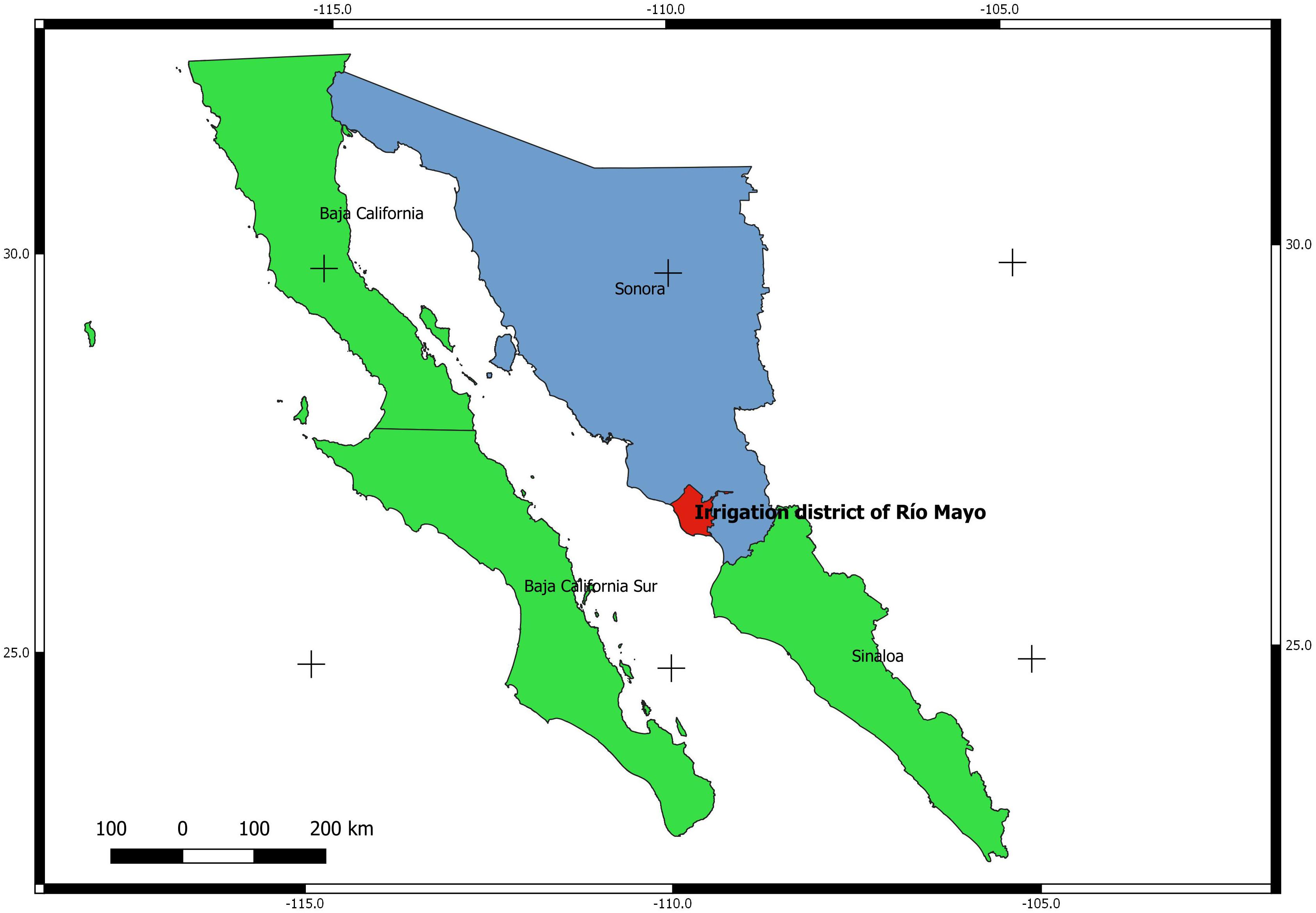
Figure 1. Study zone Irrigation District of Río Mayo, located in the southwest of Sonora and draining directly to the Gulf of California.

According to Conagua (2017), wheat was the main crop, with more than 73% of the total area for the autumn–winter 2015–2016 cycle in the irrigation district, while for the spring–summer cultivation cycle, the main crops were corn and safflower. For the studied area, the use of nitrogen ranges between 150 and 400 kg/ha for the cultivation of wheat, with an average of 250 kg/ha (Matson et al., 1998; Harrison and Matson, 2003; Beman et al., 2005; Harrison et al., 2005; Armenta-Bojórquez et al., 2012).

Overall Research Design

The methodology implemented in this manuscript is shown in Figure 2. We separated the methodology into the following parts: hydrological characterization (blue), land cover classification (green), selection and validation of the image (orange), estimation of the total of nitrogen runoff to the coastal zone (red and purple), and confirmation of determination using MODIS K_d(490) estimated values for zones around the entry point. These parts are explained in the following sections.

FIGURE 2

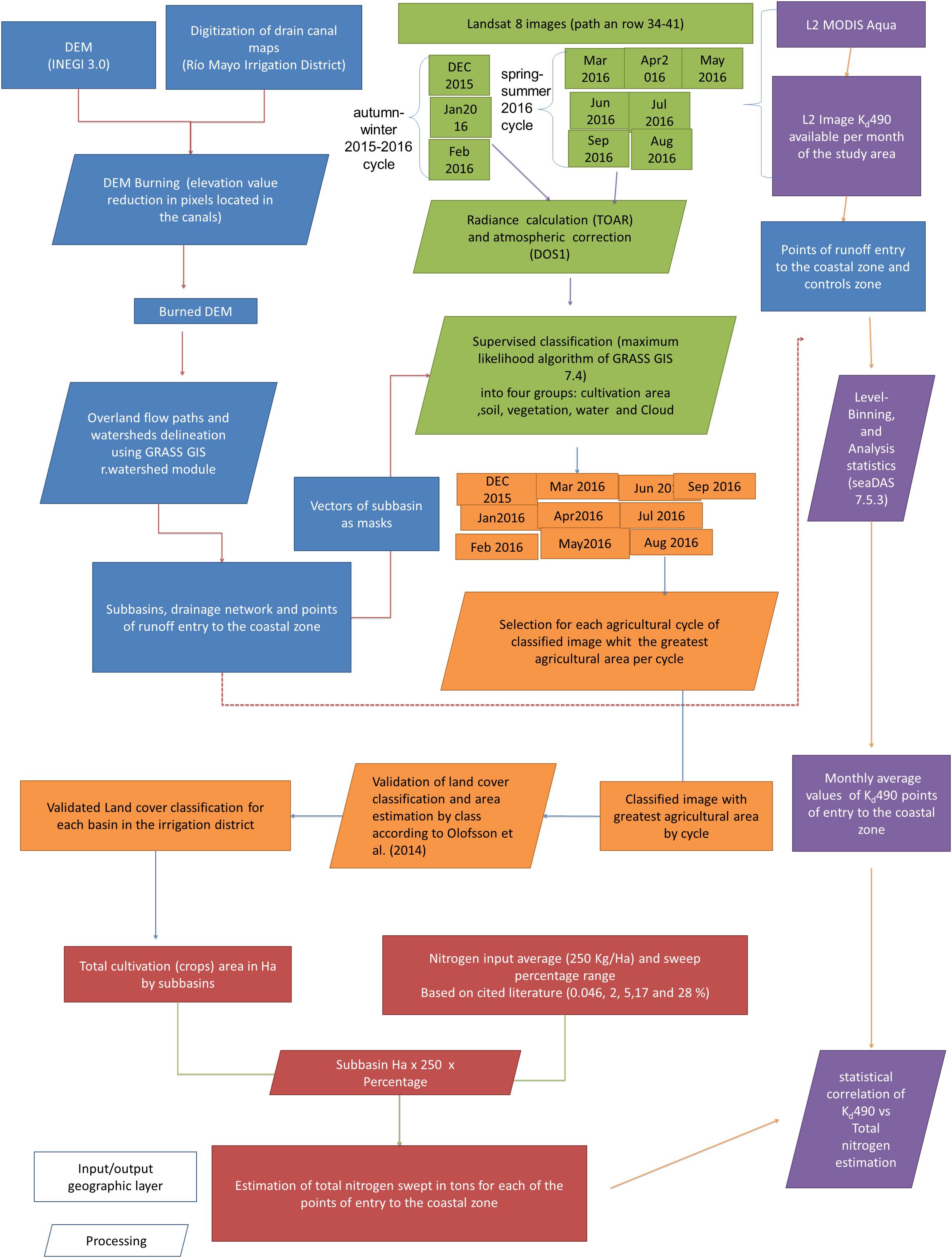
Figure 2. Methodology flowchart for estimating nitrogen runoff from crops to the coastal zones.

Hydrological Analysis

Allocation of Runoff Marine Entry Points

In order to determine the marine runoff entry points, the hydrological connectivity, and the sub-basins, we used the elevation model Contínuo de Elevaciones Mexicano 3.0 at 15 m, obtained from INEGI (2017). This model was adjusted (“burned,” i.e., reducing the elevation value in the pixels) in the parts corresponding to the canal maps digitized from the irrigation district page (Mayo, 2016) to make sure that the drainage network obtained by the model matched the actual channel network. This process was done using the software QGIS 2.18.16 (QGIS Development Team, 2018). To model the course followed by the runoff in each of the agricultural areas, we used the r.watershed module of the GRASS GIS 7.4 software with a limit parameter (flow accumulation threshold value) of 500 cells. For the watersheds, a threshold of 1,000 cells was used. These thresholds were selected to obtain the drainage network, as well as the watersheds formed for each of these networks within the study area.

Precipitation Patterns Analysis

The periods and volume of precipitation measured at the stations located in the area of study were obtained from the database of the National Climatological Observatory of Mexico’s National Meteorological Service (SMN, 2018) and from data of climatological activity between 2015 and 2016 from the INIFAP (2018).

Land Cover Classification to Detect Planted Areas

To determine the total planted agricultural area, the classification must represent the maximum agricultural area per cycle; in this case, the maximums corresponded to the months of February, 2016 and September, 2016. Therefore, previously made classifications cannot be used, since the agricultural area can change in each season. For this reason, we used Landsat 8 images path and row (34–41). Landsat images are open access and offer enough resolution for the land cover determination without needing to compose an image for study zones. The selected images corresponded to the two agricultural cycles: autumn–winter 2015–2016 and spring–summer 2016 (one per month). The Supplementary Appendix shows the images that were used. The digital level values of all the images were converted to Top of Atmosphere Radiance (TOAR). We used the Dark Object Subtraction (DOS1) method in QGIS 2.18 to correct for atmospheric effects.

In order to obtain the total planted area per season, as well as its geographical location, we used supervised classification (maximum likelihood algorithm of GRASS GIS 7.4), and each image was categorized into four groups: cultivation area (all the parcels that are photosynthetic active), soil (land or parcel that has no use or vegetation), vegetation (mangle, bushes, or surrounding trees), and water (shrimp farms, estuaries, coastal lagoons), while for the image that corresponds to the autumn–winter cycle, due to a small area with clouds close to 5% of the studied zone, we added a fifth class (cloud). As a result of the classification, we obtained the plots belonging to a basin and its drainage outlet.

Validation of Land Cover Classification

We used the method proposed by Olofsson et al. (2014) to validate the classification for the entire irrigation district of the Río Mayo, as well as for each of the determined sub-basins. This method includes calculating the sample size and assigning it in the categories of coverage types, based on the best result of five hypothetical assignments. Olofsson et al. (2014) suggest using Cochran’s (Cochran, 1997) formula to calculate sample size (η):

$$\mathrm{\eta }\approx {\left(\frac{W_i{\text{S}}_i}{\text{S}(\stackrel{\mathrm{\wedge }}{O)}}\right)}^2(1)$$

where $\text{S}(\stackrel{\mathrm{\wedge }}{O)}$ is the standard error of the estimated overall accuracy that we would like to achieve, W_i is the mapped proportion of area of class i, and S_i is the standard deviation of stratum i, calculated according to Cochran’s formula (1977) as:

$$S_i=\sqrt{U_i(1-U_i)}(2)$$

where U_i is the user’s accuracy of class i (the proportion of the area mapped as class I that has reference class I: cultivation area S(Û_ca), soil S(Û_s), vegetation S(Û_v), water S(Û_w), and cloud S(Û_c). We used an SS(Ô) of 0.015 for the sample size calculation.

To determine sample allocation to strata, Olofsson et al. (2014) suggest allocating a sample size of 50–100 for each change strata, using the variance estimator for user’s accuracy $\widehat{V}$[$\widehat{V}\left(\widehat{U_i}\right)$, Equation 3] to decide the sample size needed to achieve certain standard errors for the assumed estimated user’s accuracy for that class.

$$\widehat{V}\left(\widehat{U_i}\right)=\widehat{U_i}(1-\widehat{U_i})/n_i-1)(3)$$

where n_i is the sample size allocated to class i. Olofsson et al. (2014) indicate that n–r sample units remain after a sample size of r units has been allocated to the rare class strata. They suggest allocating the sample size of n–r proportionally to the area of each remaining stratum. As a next step, they point out that the anticipated estimated variances can be computed (based on the sample size allocation) for user’s and overall accuracy and area using following Equations (3)–(5).

$$\widehat{V}\left(\widehat{O}\right)=\sum _{1=1}^q{W}_i^2\widehat{U_i}(1-\widehat{U_i})/n_i-1)(4)$$

where $\widehat{V}\left(\widehat{O}\right)$ is the estimated variance for overall accuracy.

$$S({\widehat{P}}_{.k})=\sqrt{\sum \frac{W{\widehat{P}}_{ik}-{\widehat{P}}_{ik}^2}{ni-1}}(5)$$

where $S({\widehat{P}}_{.k})$ is the standard error of the proportion of area mapped as class k.

In particular, five possible “allocations” were constructed for each watershed, with an average of 613 samples, distributed in four classes for the month of February. For the month of September, averages of 790 samples were allocated in the five classes.

Determination of Reference Data

After having selected the best sample allocation to strata, the reference data to validate the classification was obtained by the following procedure. A visual inspection of each of the sample units was performed to assign the reference land cover type using the true color composite of the used Landsat images, together with corresponding Google Earth^TM imagery. For February, the reference data had a month of difference and 2 months difference for September. This was based on the availability of Google imagery. A random allocation of the points defined as n_i was performed using QGis 2.18.

Estimating Accuracy, Area, and Confidence Intervals of Plated Areas

We used the method proposed by Olofsson et al. (2014) to estimate accuracy, area, and confidence intervals for each category. We calculated the area estimation error (${\widehat{P}}_{.k}$, Equation 6) and the pixel precision using the confusion matrix (Supplementary Appendix) relative to the confidence intervals using the following equations [$S\left({\widehat{A}}_n\right)$ and ${\widehat{A}}_n$, Equations 7 and 8].

$${\widehat{P}}_{.k}=\sum _{i=1}^q{W}_i\frac{n_{iK}}{n_i}(6)$$

$$S({\widehat{A}}_n)=S({\widehat{P}}_{.k})x\times A_{tot}{A}_{\text{tot}}xz(7)$$

$${\widehat{A}}_n={\widehat{P}}_{.k}x\times A_{tot}{A}_{\text{tot}}(8)$$

where $S({\widehat{A}}_n)$ is the error for the estimated area, z = 1.96 is the confidence interval at 95%, and A_totA_tot is the total of pixels, while ${\widehat{A}}_n$ is the estimated area for the class n.

This procedure was followed for both the total area of the study basin and for each of the sub-basins previously determined, using a confidence interval of 95%.

Estimation of Amount of Nitrogen Used for Main Crops in the Area of Study

The volume of nitrogen from runoff was obtained by multiplying the cultivated area by the average of nitrogen reported (250 kg/ha) and by the percentage of nitrogen in the runoff water according to the values of Riley et al. (2001). In addition, Mexican official recommendations and sowing manuals (SAGARPA, 2015) were used to obtain doses of nitrogen used for the main crops of the area during the periods studied.

Analysis of the Diffuse Attenuation Coefficient K_d(490) Concentration Around the Coastal Entry Points

Satellite images of the diffuse attenuation coefficient at 490 nm K_d(490) L2 OCI were obtained for the two crop cycles from the Moderate Resolution Imaging Spectroradiometer (MODIS-AQUA) from the Ocean Color Data Browser (NASA, 2019b). To obtain the monthly average with a 1 km resolution pixel and to extract the data and for the composed monthly average K_d(490) image for each of the coastal entry points of nutrients previously determined and two control zones (areas where there are no agricultural plots nearby), we used the L2-binnig module of the software seaDAS version 7.5.3 (NASA, 2019a). Each sampling had an area of 19.6 km². This information was used to confirm the amount of nitrogen runoff received by the marine coastal zones through the entry points.

Validation of the Nitrogen Estimation Method

To validate the proposed method to estimate nitrogen inputs in the marine zone, a statistical correlation between the estimated values of nitrogen runoff for each basin and the satellite K_d(490) values around its corresponding outlet point (marine entry point) was performed in R. For this end, we used the 2% nitrogen concentration values.

Results

Hydrological Analysis

The obtained drainage lines, the basins, and the estimated nutrient entry points along the coastal zone and the coastal lagoons are shown in Figure 3. Eight basins were obtained within the irrigation district (shown in Figure 3 with different colors). They allowed a determination of which agricultural parcels drain to the same area. The entry points allow allocation of the affected coastal zone and the coastal lagoons. The results indicate that there are some direct entry points to the Gulf of California, while others are located between mangrove areas and the lagoon of Yavaros and Tóbari.

FIGURE 3

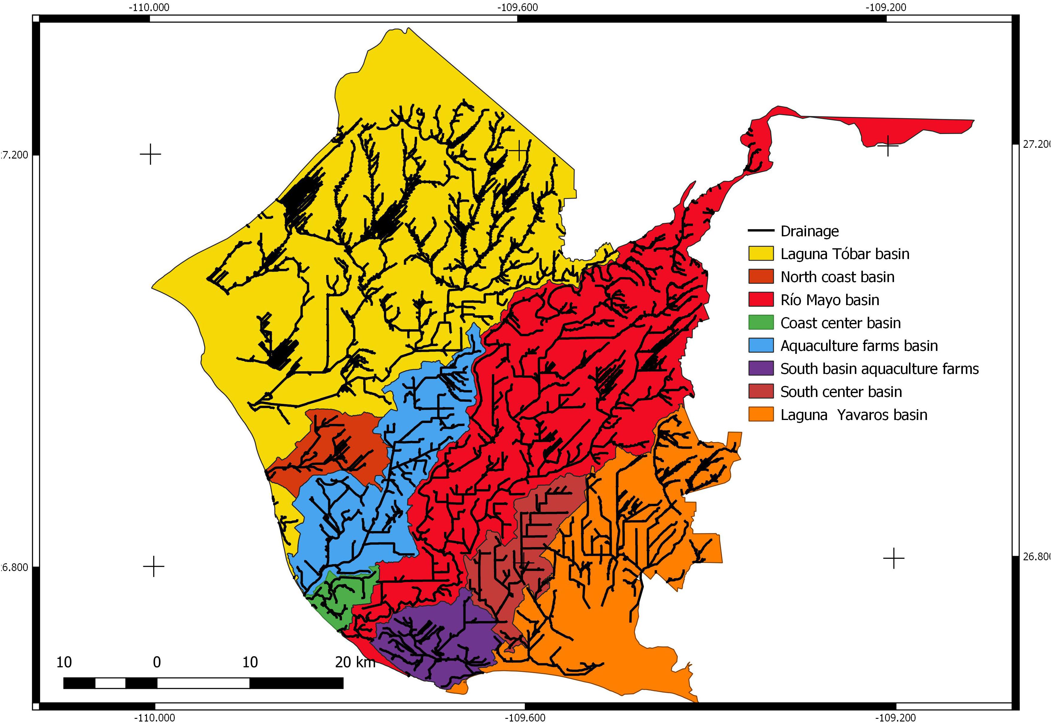
Figure 3. Drainage lines calculated in black along with the main points of entry of nutrients, superimposed with the eight hydrological basins determined for the region of the Irrigation District of the Río Mayo. On the upper right corner, a Landsat 543 band combination is shown.

The results for the two agricultural cycles indicate that rainfall was scarce, and that even during the rainy seasons, there was no total monthly rainfall >130 mm (Figure 4) nor maximum daily rainfall >35 mm. Thus, it can be stated that the relative contribution of precipitation during these two agricultural periods was of low importance regarding the runoff of nutrients into the coastal zone, which depends mainly on the water from the Adolfo Ruiz Cortines dam, together with the various extraction wells used for irrigation.

FIGURE 4

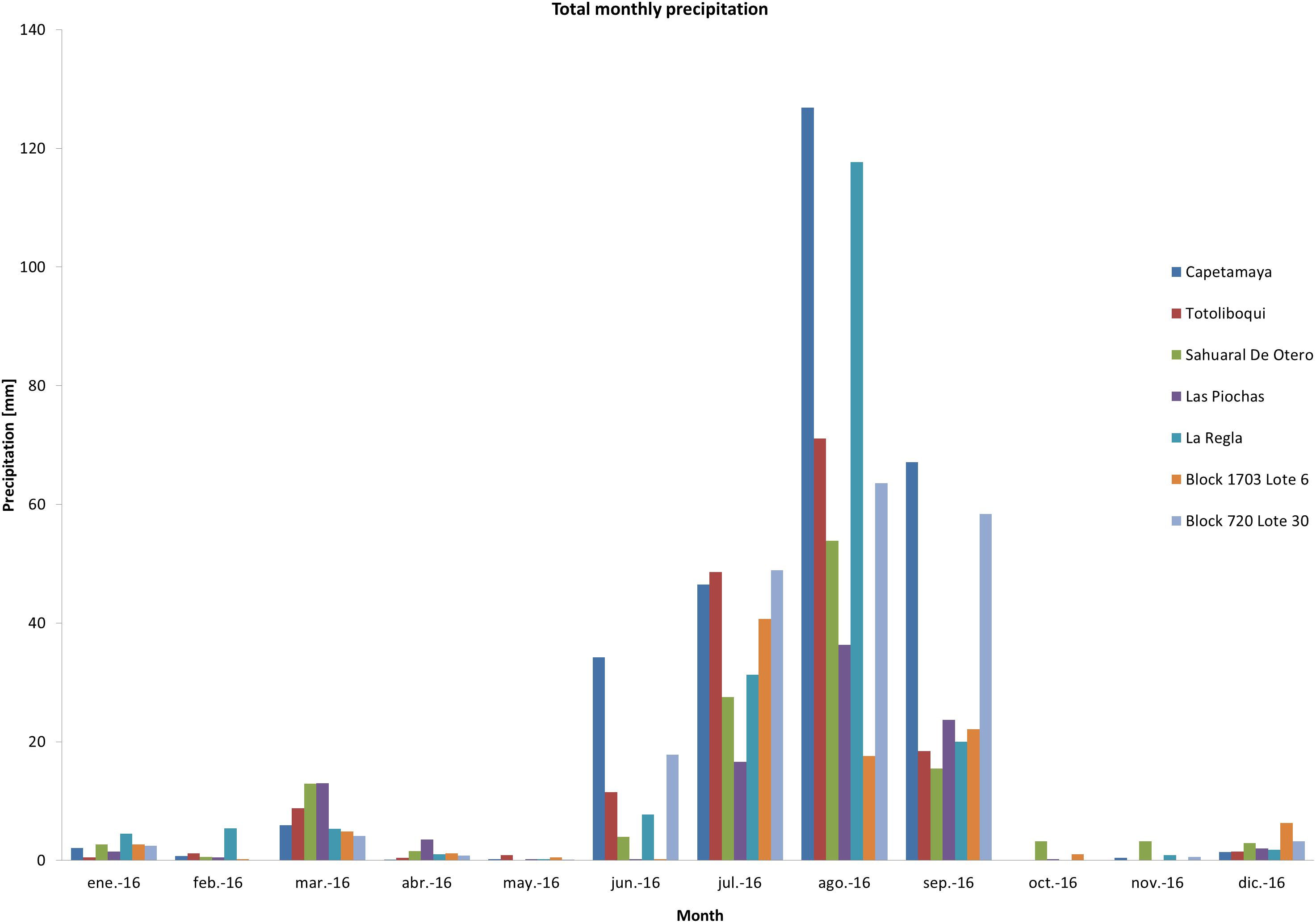
Figure 4. Total monthly precipitation in millimeters measured at weather stations for the Río Mayo Irrigation District during the 2016 period. Of these seven weather stations, four are in the studied zone: Sahuaral De Otero in the North Costa basin and near the aquaculture farms basin, Las Piochasand Capetamaya in the Río Mayo basin, and La Regla in the Yavaros Laguna Yavaros basin.

Identification and Estimation of the Agricultural Areas

After image classification, Table 1 shows the number of classes used, number of samplings, standard error of the estimated overall accuracy, selected accuracy of the allocation that was chosen, and estimated user’s accuracy for each class for all selected allocations of each basin. It also shows all the allocation variables selected for each sub-basin. In the case of the autumn–winter cycle, the selection was based on the smallest estimated user’s accuracy for the cultivation area and the soil area, while for the spring–summer cycle, priority was given to soil and cultivation area, in that order.

TABLE 1

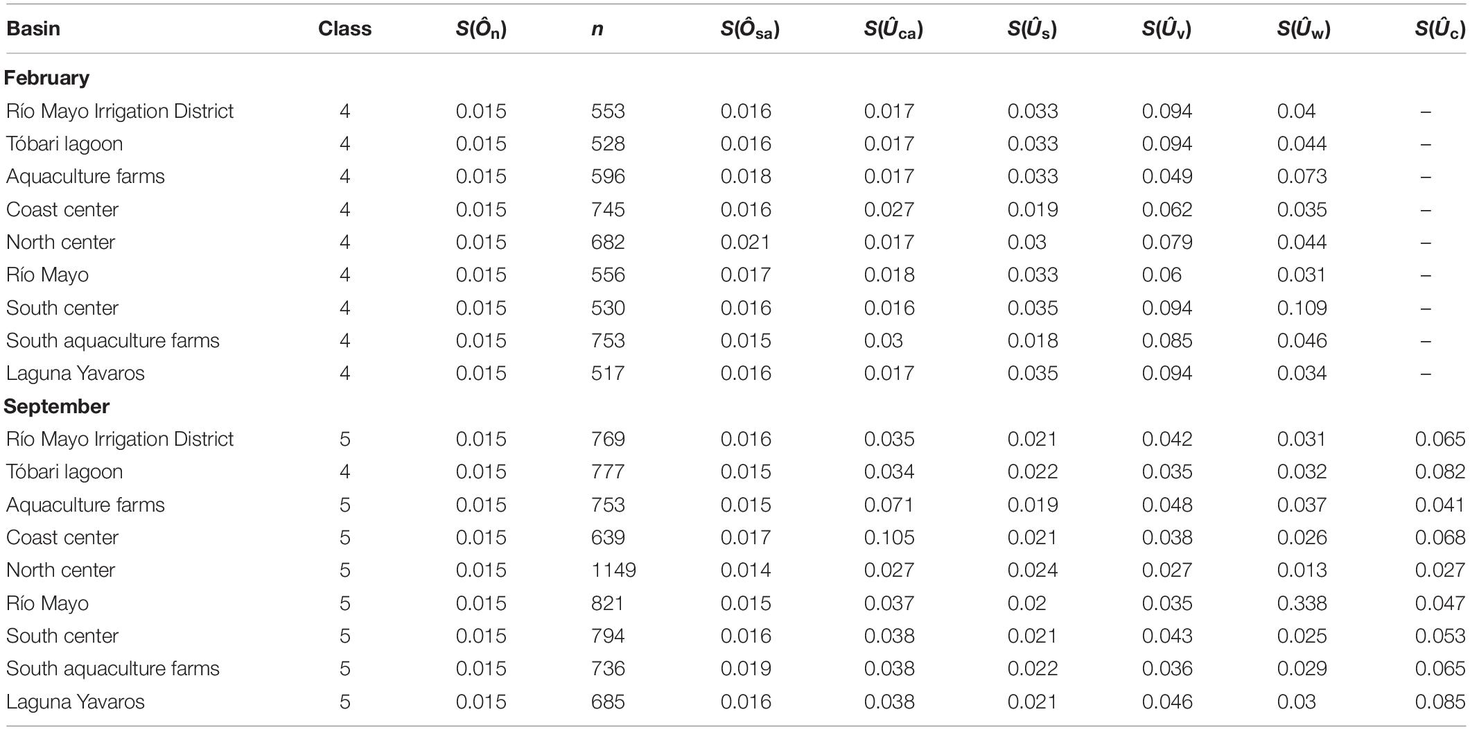
Table 1. Number of classes by sub-basin, sampling number (n), standard error of the estimated overall accuracy S(Ô_n), selected accuracy S(Ô_sa) of the allocation that was chosen, and estimated user’s accuracy for each class SÛ_i.

As example, tables showing data of the entire irrigation district are included in Supplementary Appendix. As mentioned, these determinations were done for all sub-basins and for the entire district. Table 1 of the Supplementary Appendix shows the standard errors of the user’s and overall accuracies for the five possible allocations. We selected allocation 3 for the autumn–winter cycle (February) and allocation 1 for the spring–summer cycle (September), due to their lowest values in the standard error for cultivation area, soil, and selected accuracy. Table 2 shows the estimator matrix for the total of the Río Mayo irrigation district for February and September, while Table 4 of the Supplementary Appendix shows the error matrix of sample counts of each allocation.

TABLE 2

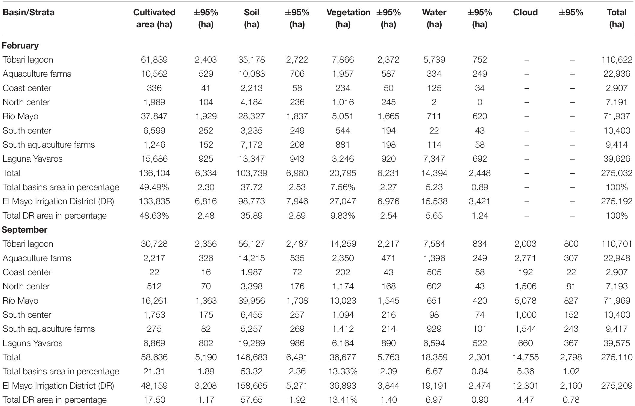
Table 2. Area that covers each class, as well as its estimation error.

Estimation of Nitrogen Runoff

Table 2 shows all data from the validation classification for each sub-basin and the entire irrigation district for the two cycles, and all the basins with their estimation error for each strata. The large difference in the land used in each cycle should be noted. While the autumn–winter had more than 49% of the total areas as cultivated category and the category of soil represents almost 38% of this proportion change, for the spring–summer cycle, the main category is soil, with more than 57% of all the irrigation district and the cultivation category representing just 21.3%. Table 3 shows the percentages of nitrogen runoff reported by Riley et al. (2001), multiplied by the planted area obtained after classification. The irrigation district Río Mayo basin has its main cultivation period in the autumn–winter cycle, although it also has important nitrogen contributions during the spring–summer cycle. The Tóbari lagoon basin has the most agricultural land cover in both the autumn–winter cycle and spring–summer cycle, and with discharge into the Tóbari lagoon. The Río Mayo basin is second in agricultural production and volume of nitrogen runoff. This basin discharges directly to the Gulf of California. While the Tóbari lagoon basin has a minor agricultural contribution, it also receives input from the shrimp farms that are in the area.

TABLE 3

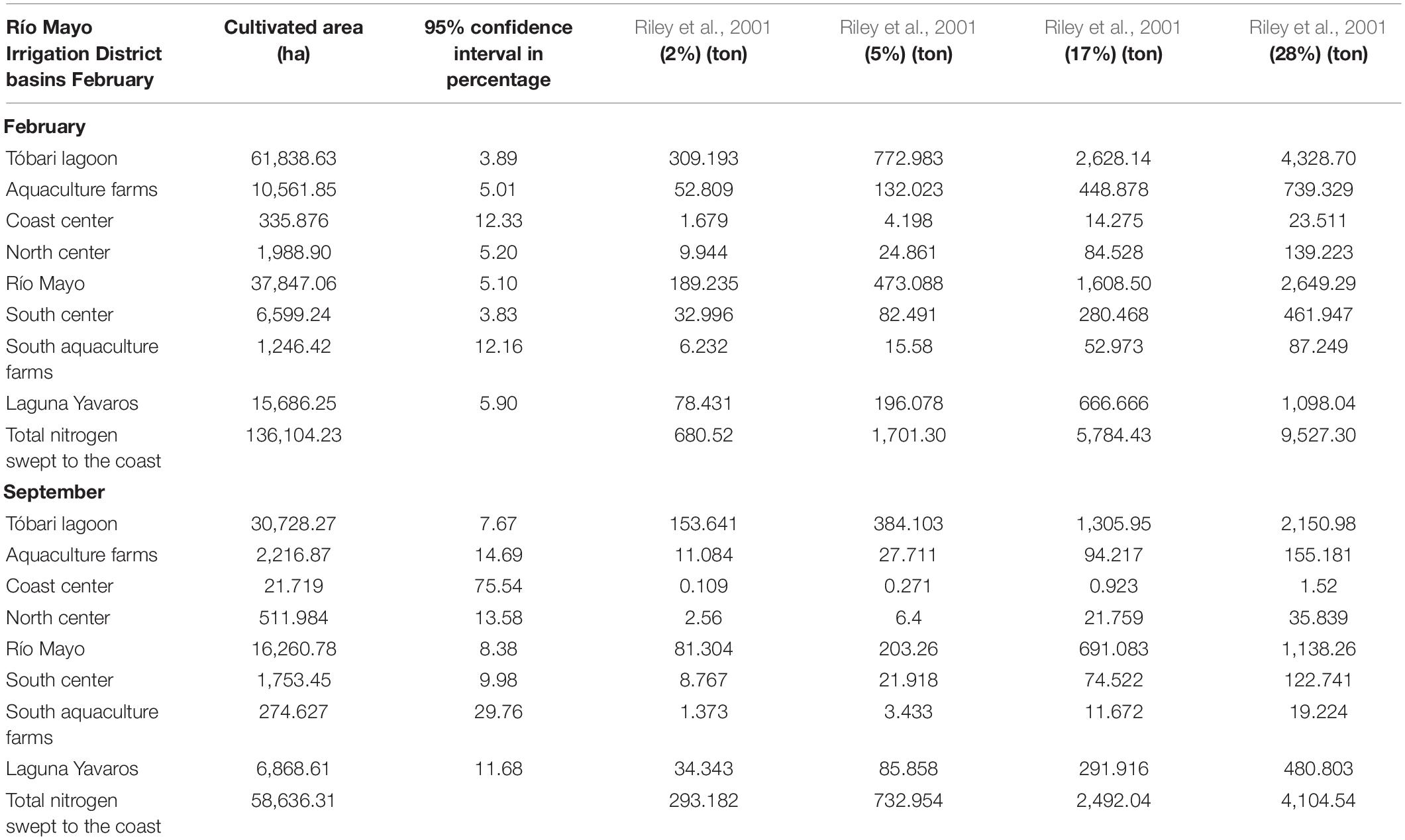
Table 3. Estimate of nitrogen from runoff according to the average used in the literature of 250 kg/ha, as well as estimates of sweep percentage according to the cited literature.

Analysis and Validation of the Nitrogen Estimation Method

Figure 5 shows the K_d(490) values for each of the entry points of nutrients to the coastal zone by month for the two agricultural cycles. We confirmed that the higher clarity of coastal zones water correspond to the control zones, while the lower correspond to the main agricultural areas.

FIGURE 5

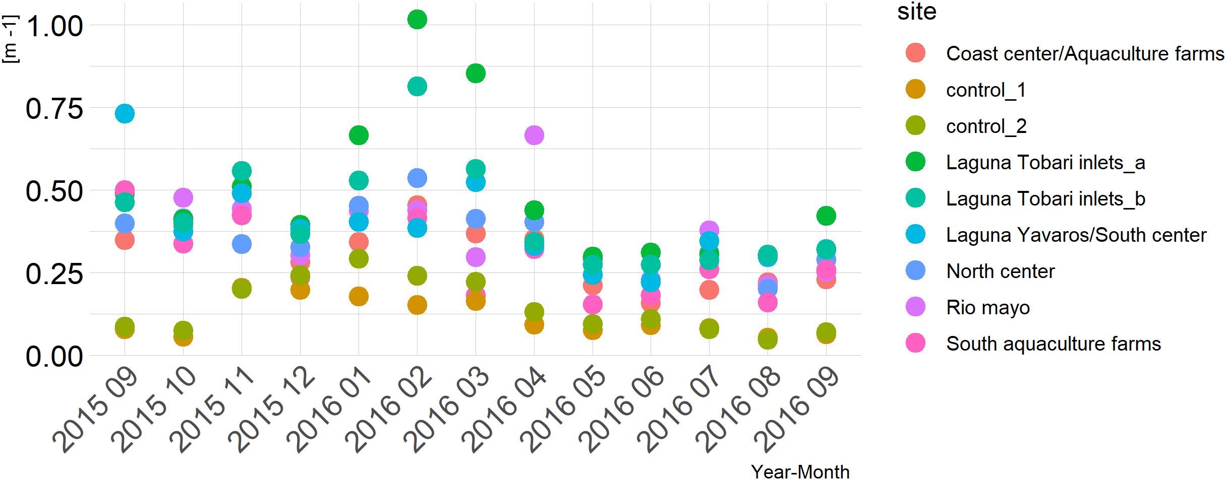
Figure 5. K_d(490) values for each of the entry points of nutrients to the coastal zone by month for the two agricultural cycles.

In addition, as the data did not fulfill the assumptions of normality and homoscedasticity, a non-parametric test was used. The Spearman correlation analysis (see Figure 6) indicate a significant correlation (autumn–winter: r = 0.705, p = 0.002, spring–summer: r = 0.678, p = 0.003) between the K_d(490) and the nitrogen values. This is very promising for the rapid method proposed here to estimate effects of agriculture farms into the coastal zone. The plots consistently show for both agricultural seasons that the order of the highest and lowest compared values is the same. The controls (basins without agricultural influence) have the lowest values of the compared correlated parameters, and the highest values are registered for the Tóbari lagoon basin.

FIGURE 6

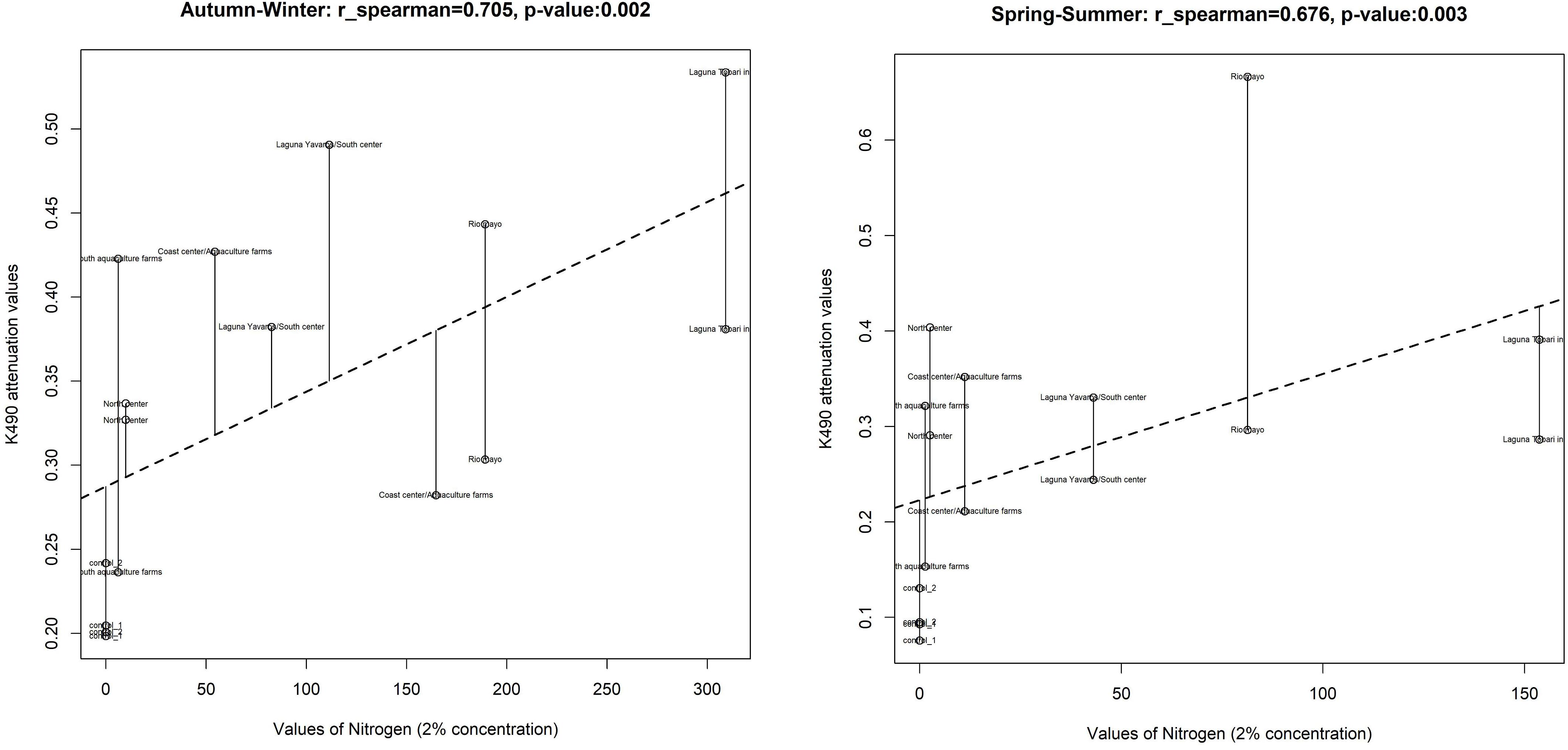
Figure 6. The correlation analysis between the Kd(490) and the runoff nitrogen values for both agricultural cycles.

Discussion

This study provides a robust starting point for the quantification and estimation of total nitrogen from runoffs into the coastal area, especially in zones where the information is not available or incomplete, unlike others models (McClelland et al., 1997; Valiela et al., 1997; Hofmeister et al., 2016; Sun et al., 2016) that require different layers of information (e.g., type of soil, topography wetness index, floodwater depth, among others) and concede the input of other variables, such as using stable nitrogen isotopes, to distinguish the sources, leaching, and availability (Teichberg et al., 2008; Ochoa-Izaguirre and Soto-Jiménez, 2013; Viana and Bode, 2013; Rivero-Villar et al., 2018).

One of the main advantages of the Olofsson et al. (2014) method to validate land use and land cover classifications is that it considers confidence intervals for the quantification of the cultivated area, allowing a statistical interpretation of the estimates of the nitrogen concentrations from runoff. We believe that, when selecting the data with the largest cultivated area of the season, we obtained data that are closer and more representative of the amount of total cultivated plot found in each basin. One of the main problems for the classification of crops/soils that we experienced was the presence of clouds, since they can mask or increase the classification error for the other class. As shown in Table 3, the estimation error is close to 19% of the total cloud classification, even though this specific class only represents <5% of the overall classification, and the main class cultivated area for February and soil for September only had 4.6 and 4.25% of estimation error, respectively.

Another important result is the geographical location of the drainage entry points. The possible effect of drainage on the ecosystems can be estimated, depending on whether there are buffer zones or nutrient traps, as would be the case of a wetland or a direct entry to the coastal zone (Figure 3). Knowing the location of nutrient entry points allows the implementation of action plans and public policies to address the problem of eutrophication and agricultural pollution. For example, the Tóbari lagoon receives contributions from livestock, urban waste waters, shrimp farms, and two irrigation districts (Valle del Yaqui irrigation district and Río Mayo) (Ahrens et al., 2008; Páez-Osuna et al., 2017). In the same line, Ruiz-Ruiz (2017) describes how the Tóbari lagoon presented a biological stress and even hypoxia during the summer of 2012, while Vargas-González (2018) explains how the discharge waters from the agricultural parcels have an effect on the salinity of the Yavaros lagoon and report the presence of Aldrin and other pesticides in this lagoon.

With the results obtained from this study and the analysis of the nutrient entry points to the coast, we have identified that two basins are the most important in terms of agricultural production and the entry of nutrients: Tóbari lagoon and the basin of Río Mayo. For the purpose of study, the great majority of nutrients that reach these coastal areas arrive during the periods of irrigation, since rainfall is scarce year round (Figure 4). A large contribution of nitrogen was probably during the first irrigation, according to the planting manuals (SAGARPA, 2015). During this period, the crop already has ∼60–80% of the total fertilizer to be used during the crop cycle.

As stated by Ahrens et al. (2008); Ruiz-Ruiz (2017), Páez-Osuna et al. (2017), and Vargas-González (2018), the Tóbari lagoon is exposed to a combination of diverse anthropogenic pressures. As one of the main vectors of nitrogen, agricultural runoff can have a significant input to this lagoon, depending on whether there was a previous study of nitrogen soil available. For example, with the lowest estimates of 2% of fertilizer runoff to the Tóbari basin for the autumn–winter cycle, ∼680 tons of nitrogen could enter the lagoon in the first months of planting. In the case of the upper estimates, there was not a previous soil–nitrogen study, but the volume of nitrogen that could enter the Tóbari lagoon could even go to the upper limit of 27%. That means more than 4,000 tons would have reached the basin, which highlights the need for more study of the relationship between agricultural and coastal zones.

Within the values of K_d(490) that we obtained (Figure 5), it is of interest to note that the lower clarity correspond to areas where there is great contribution of nutrients and other compounds from the field. It is important to note that agricultural and aquacultural activities are well reported as a main pathway for organic matter and other compounds to the coastal zones (Beman et al., 2005; Ahrens et al., 2008; Páez-Osuna et al., 2017). In contrast, the values of the control zone remain with a high transparency, during the two agricultural cycles, having a peak of increased turbidity during the months of December and March.

Reviewing studies such as that of Beman et al. (2005), and the data obtained in this work, allows us to think that agricultural runoff in the Gulf of California can have a greater influence in this area. Particularly, the results obtained show that the Río Mayo basin is contributing a large amount of agricultural substances directly to the coastal zone into the Gulf of California, since there is not sufficient filtration or retention of nutrients and contaminants. Therefore, its entry and dissemination to the marine area could have several ecological implications.

It is worth noting that there is daily use of high amounts of fertilizers, which are high in nitrogen, within the Sonoran agricultural area, as indicated by Beman et al. (2005) and Christensen et al. (2006). This can also be seen when analyzing the recommendations for the use of nitrogen for the main crops, within the manuals published by SAGARPA (2015) for Sonora.

Additionally, we proved that the methodology can provide a cost-effective, practical approach for estimating nitrogen entries into coastal zones and can be also applied to estimate the runoff of other contaminants. This would allow better decision-making regarding the interaction between agricultural zones and coastal areas.

Conclusion

We developed an easy and rapid GIS and remote sensing-based method that uses open access data to estimate nitrogen or any contaminant that changes the optic water properties and that is swept into the coastal zone. The superficial connectivity analysis model used in this study allowed the estimation of nitrogen input to the coastal zones. The developed method allows incorporating field data and extrapolating to any agricultural area.

With the results obtained in this study, we conclude that the quantities of nitrogen fertilizer that enter the coastal zone from the agricultural runoff have an ecological effect by decreasing the clarity of water in the coastal zone. It is undeniable that there is an input of nutrients and other pollutants from both the irrigation districts of the Río Mayo and other agricultural areas. It is therefore necessary to have tools that allow rapid quantification and analysis to create public policies that will protect the Gulf of California. We propose that these results and this methodology can help to create an easy and quicker agricultural runoff nitrogen inventory for the coastal zone of the Gulf of California and other marine coastal zones worldwide.

Data Availability Statement

The datasets generated for this study are available on request to the corresponding author.

Author Contributions

DG-R, FT-S, DR-F, and AO-R significantly contributed to the conception and design of the study. DG-R, FT-S, JB-G, and LB-M organized the databases and the satellite image processing. DG-R, FT-S, and DL-C performed the statistical analysis. DG-R and FT-S contributed to wrote the first draft of the manuscript. DR-F, FT-S, DR-F, JB-G, LB-M, DL-C, and AO-R wrote specific sections of the manuscript. All authors contributed to the manuscript revision, read, and approved the submitted version.

Funding

This work was supported by the Consejo Nacional de Ciencia y Tecnología (CONACYT) Projects: 251919 and 293368.

Conflict of Interest

The authors declare that the research was conducted in the absence of any commercial or financial relationships that could be construed as a potential conflict of interest.

Acknowledgments

We acknowledge the CIBNOR-CONACYT doctoral program in science. “Use, Management” and Preservation of Natural Resources for scholarship number 419362. This study was developed with the financial support of Project 293368 of Natural Protected Areas Thematic Networks and Project 251919 of Basic Science of CONACYT. We aknowledge Charlotte Smith and Ms. Susan Drier-Jonas for comments on the manuscript as well as two reviewers: Antonio Bode and Raul Martell-Dubois and the associate editor Alejandro Jose Souza for all their time an effort devoted to improve earlier versions of our manuscript.

Supplementary Material

The Supplementary Material for this article can be found online at: https://www.frontiersin.org/articles/10.3389/fmars.2020.00316/full#supplementary-material

References

Ahrens, T. D., Beman, J. M., Harrison, J. A., Jewett, P. K., and Matson, P. A. (2008). A synthesis of nitrogen transformations and transfers from land to the sea in the Yaqui Valley agricultural region of northwest Mexico. Water Resour. Res. 44:41. doi: 10.1029/2007WR006661

CrossRef Full Text | Google Scholar

Armenta-Bojórquez, A. D., Cervantes-Medina, C., Galaviz-Lara, J. A., Camacho-Báez, J., Mundo-Ocampo, M., and García-Gutiérrez, C. (2012). Impacto de la fertilización nitrogenada en agua para consumo humano en el municipio de Guasave Sinaloa. Ra Ximhai 8, 11–16.

Google Scholar

Beman, M. J., Arrigo, K. R., and Matson, P. A. (2005). Agricultural runoff fuels large phytoplankton blooms in vulnerable areas of the ocean. Nature 434:211. doi: 10.1038/nature03370

PubMed Abstract | CrossRef Full Text | Google Scholar

Breitburg, D., Levin, L. A., and Oschlies, A. (2018). Declining oxygen in the global ocean and coastal waters. Science 359:eaam7240. doi: 10.1126/science.aam7240

PubMed Abstract | CrossRef Full Text | Google Scholar

Chang, H. (2008). Spatial analysis of water quality trends in the Han River basin, South Korea. Water Res. 42, 3285–3304. doi: 10.1016/j.watres.2008.04.006

PubMed Abstract | CrossRef Full Text | Google Scholar

Christensen, L., Riley, W. J., and Ortiz-Monasterio, I. (2006). Nitrogen Cycling in an Irrigated Wheat System in Sonora, Mexico: measurements and Modeling. Nutr. Cycl. Agroecosyst. 75, 175–186. doi: 10.1007/s10705-006-9025-y

CrossRef Full Text | Google Scholar

Cochran, W. G. (1997). Sampling Techniques, 3rd Edn. Hoboken, NJ: John Wiley.

Google Scholar

Conagua, S. (2017). Estadísticas Agrícolas de los Distritos de Riego Año Agrícola 2015-2016. Ciudad de México: Comisión Nacional del Agua.

Google Scholar

Davidson, K., Gowen, R. J., Harrison, P. J., Fleming, L. E., Hoagland, P., Moschonas, G., et al. (2014). Anthropogenic nutrients and harmful algae in coastal waters. J. Environ. Manag. 146, 206–216. doi: 10.1016/j.jenvman.2014.07.002

PubMed Abstract | CrossRef Full Text | Google Scholar

Harrison, J., and Matson, P. (2003). Patterns and controls of nitrous oxide emissions from waters draining a subtropical agricultural valley. Glob. Biogeochem. Cycles 17:91. doi: 10.1029/2002GB001991

CrossRef Full Text | Google Scholar

Harrison, J. A., Matson, P. A., and Fendorf, S. E. (2005). Effects of a diel oxygen cycle on nitrogen transformations and greenhouse gas emissions in a eutrophied subtropical stream. Aquat. Sci. 67, 308–315. doi: 10.1007/s00027-005-0776-773

CrossRef Full Text | Google Scholar

He, C., and DeMarchi, C. (2014). Modeling spatial distributions of point and nonpoint source pollution loadings in the Great Lakes Watersheds. Int. J. Environ. Sci. Eng. 2:1.

Google Scholar

Hofmeister, K. L., Georgakakos, C. B., and Walter, M. T. (2016). A runoff risk model based on topographic wetness indices and probability distributions of rainfall and soil moisture for central New York agricultural fields. J. Soil Water Conserv. 71, 289–300. doi: 10.2489/jswc.71.4.289

CrossRef Full Text | Google Scholar

INEGI, (2017). Continuo de Elevaciones Mexicano 3.0. Available online at: http://www.beta.inegi.org.mx/temas/mapas/relieve/continental/ (accessed January, 2017).

Google Scholar

INIFAP, (2018). Red Nacional de Estaciones Agrometeorológicas Automatizadas INIFAP. Available online at: https://clima.inifap.gob.mx/lnmysr/Estaciones/MapaEstaciones (accessed February, 2018).

Google Scholar

López-Vicente, M., García-Ruiz, R., and Guzmán, G. (2016). Temporal stability and patterns of runoff and runon with different cover crops in an olive orchard (SW Andalusia, Spain). CATENA 147, 125–137. doi: 10.1016/j.catena.2016.07.002

CrossRef Full Text | Google Scholar

Lorenzana-Durán, G. (2004). Un garbanzo de a Libra: Agricultura comercial en el valle del Mayo, 1884-1910. Guanajuato: Asociación Mexicana de Historia Económica A. C.

Google Scholar

Mainali, J., and Chang, H. (2018). Landscape and anthropogenic factors affecting spatial patterns of water quality trends in a large river basin, South Korea. J. Hydrol. 564, 26–40. doi: 10.1016/j.jhydrol.2018.06.074

CrossRef Full Text | Google Scholar

Matson, P. A., Naylor, R., and Ortiz-Monasterio, I. (1998). Integration of environmental, agronomic, and economic aspects of fertilizer management. Science 280:112. doi: 10.1126/science.280.5360.112

PubMed Abstract | CrossRef Full Text | Google Scholar

Mayo, (2016). Distrito de Riego Del Río Mayo. Available online at: http://drrmayo.mx/ (accessed December, 2016).

Google Scholar

McClelland, J. W., Valiela, I., and Michener, R. H. (1997). Nitrogen-stable isotope signatures in estuarine food webs: A record of increasing urbanization in coastal watersheds. Limnol. Oceanogr. 42, 930–937. doi: 10.4319/lo.1997.42.5.0930

CrossRef Full Text | Google Scholar

Montes, A. M., González-Farias, F. A., and Botello, A. V. (2012). Pollution by organochlorine pesticides in Navachiste-Macapule, Sinaloa, Mexico. Environ. Monit. Assess 184, 1359–1369. doi: 10.1007/s10661-011-2046-2

PubMed Abstract | CrossRef Full Text | Google Scholar

Mouri, G., Shinoda, S., and Oki, T. (2010). Estimation of total nitrogen transport and retention during flow in a catchment using a mass balance model incorporating the effects of land cover distribution and human activity information. Water Sci. Technol. 62, 1837–1847. doi: 10.2166/wst.2010.208

PubMed Abstract | CrossRef Full Text | Google Scholar

NASA, (2019a). Available at: http://seadas.gsfc.nasa.gov/

Google Scholar

NASA, (2019b). GSFC Ocean Biology Processing Group Moderate Resolution Imaging Spectroradiometer MODIS. Washington, DC: NASA.

Google Scholar

Ochoa-Izaguirre, M. J., and Soto-Jiménez, M. F. (2013). Evaluation of nitrogen sources in the Urias lagoon system, Gulf of California, based on stable isotopes in macroalgae. Cienc. Mar. 39. doi: 10.7773/cm.v39i4.2285

CrossRef Full Text | Google Scholar

Olofsson, P., Foody, G. M., and Herold, M. (2014). Good practices for estimating area and assessing accuracy of land change. Remote Sens. Environ. 148, 42–57. doi: 10.1016/j.rse.2014.02.015

CrossRef Full Text | Google Scholar

Páez-Osuna, F., Álvarez-Borrego, S., Ruiz-Fernández, A. C., García-Hernández, J., Jara-Marini, M. E., Bergés-Tiznado, M. E., et al. (2017). Environmental status of the Gulf of California: a pollution review. Earth Sci. Rev. 166, 181–205. doi: 10.1016/j.earscirev.2017.01.014

CrossRef Full Text | Google Scholar

Pedroza-González, E., and Hinojosa-Cuéllar, G. (2014). Manejo y Distribución del Agua en Distritos de Riego: Breve Introducción Didáctica. México: Instituto Mexicano de Tecnología del Agua.

Google Scholar

Pulido Madrigal, L. (2016). Cambio climático, ensalitramiento de suelos y producción agrícola en áreas de riego. Terra Latinoamericana 34, 207–218.

Google Scholar

QGIS Development Team (2018). QGIS Geographic Information System. Open Source Geospatial Foundation Project. Available online at: http://qgis.osgeo.org

Google Scholar

Raymond, P. A., David, M. B., and Saiers, J. E. (2012). The impact of fertilization and hydrology on nitrate fluxes from Mississippi watersheds. Curr. Opin. Environ. Sustainabil. 4, 212–218. doi: 10.1016/j.cosust.2012.04.001

CrossRef Full Text | Google Scholar

Rhoads, B. L., Lewis, Q. W., and Andresen, W. (2016). Historical changes in channel network extent and channel planform in an intensively managed landscape: natural versus human-induced effects. Geomorphology 252, 17–31. doi: 10.1016/j.geomorph.2015.04.021

CrossRef Full Text | Google Scholar

Riley, W. J., Ortiz-Monasterio, I., and Matson, P. A. (2001). Nitrogen leaching and soil nitrate, nitrite, and ammonium levels under irrigated wheat in Northern Mexico. Nutr. Cycl. Agroecosyst. 61, 223–236. doi: 10.1023/A:1013758116346

CrossRef Full Text | Google Scholar

Rivero-Villar, A., Templer, P. H., Parra-Tabla, V., and Campo, J. (2018). Differences in nitrogen cycling between tropical dry forests with contrasting precipitation revealed by stable isotopes of nitrogen in plants and soils. Biotropica 50, 859–867. doi: 10.1111/btp.12612

CrossRef Full Text | Google Scholar

Ruiz-Ruiz, T. M. (2017). Análisis Comparativo de Índices de Eutrofización en Lagunas Costeras del Estado de Sonora, México. Baja California: Centro de Investigaciones Biológicas del Noroeste.

Google Scholar

SAGARPA, (2015). Agenda Técnica Agrícola de Sonora, México, Secretaría de Agricultura, Ganadería, Desarrollo Rural, Pesca y Alimentación. Méxcio: SAGARPA.

Google Scholar

SMN, (2018). Servicio Meteorológico Nacional. Available online at: https://smn.conagua.gob.mx/es/ (accessed January, 2017).

Google Scholar

Sun, X., Liang, X., Zhang, F., and Fu, C. (2016). A GIS-based upscaling estimation of nutrient runoff losses from rice paddy fields to a regional level. J. Environ. Qual. 45, 1865–1873. doi: 10.2134/jeq2016.05.0181

PubMed Abstract | CrossRef Full Text | Google Scholar

Teichberg, M., Fox, S. E., Aguila, C., Olsen, Y. S., and Valiela, I. (2008). Macroalgal responses to experimental nutrient enrichment in shallow coastal waters: growth, internal nutrient pools, and isotopic signatures. Mar. Ecol. Prog. Series 368, 117–126. doi: 10.3354/meps07564

CrossRef Full Text | Google Scholar

Valiela, I., Collins, G., Kremer, J., Lajtha, K., Geist, M., Seely, B., et al. (1997). nitrogen loading from coastal watersheds to receiving estuaries: new method and application. Ecol. App. 7, 358–380. doi: 10.1890/1051-0761(1997)007[0358:NLFCWT]2.0.CO;2

CrossRef Full Text | Google Scholar

Vargas-González, H. H. (2018). Cambio en la Biodisponibilidad de elementos traza asociados a procesos de eutrofizacion en sistemas lagunares del Golfo de California. Doctorado, Centro de Investigaciones Biológicas del Noroeste, Baja California.

Google Scholar

Viana, I. G., and Bode, A. (2013). Stable nitrogen isotopes in coastal macroalgae: geographic and anthropogenic variability. Sci. Tot. Environ. 443, 887–895. doi: 10.1016/j.scitotenv.2012.11.06

CrossRef Full Text | Google Scholar