Near-Automatic Routine Field Calibration/Correction of Glider Salinity Data Using Whitespace Maximization Image Analysis of Theta/S Data

Introduction

Ocean observing “Glider” vehicles now constitute an essential component of coastal and open ocean observing systems (Testor et al., 2019) for a number of reasons. Although flying gliders requires well-trained remote glider pilots, and deployment and recovery procedures, they are highly cost-effective compared to traditional ship-based operations. Although slower moving than a research vessel, gliders are capable of acquiring data at a high temporal and spatial resolution than was generally previously economically practical, and are able to operate even in rough sea states. In particular, the spatial and temporal resolutions of coastal data and their quality are of crucial importance to adequately respond to many scientific and societal challenges. Thus, the data collected by glider vehicles have an immensely important role in what is generically termed operational oceanography; however, to give them a legacy value for long-term historical climatologies, we must find a means to inter-calibrate (or “field correct”) their data, and we discuss this further in this section.

Now that multi-platform observations are more and more common (Tintoré et al., 2013, 2015; Bosse et al., 2015), it is further essential that inter-calibration procedures are routinely included between the data collected by different platforms. Here, metadata becomes even more important than it has been previously and must automatically be written with not just details of field correction and inter-calibrations, but also the analysis and correction of long-term sensor characteristics and drifts. The ARGO profiling float community has been aware of the requirement for inter-calibration for some time (Wong et al., 2003; Owens and Wong, 2009) and has valuable procedures in place to inter-calibrate float data as best they can. The huge growth in ocean observing data using glider vehicles provides a unique opportunity to support this initiative and take it further, particularly with the growing number of repeat monitoring lines that gliders have enabled and the resulting improvement in quasi-continuous observation of stable water masses and mode waters.

Glider vehicles are typically fitted with a payload bay equipped with the generic combination of conductivity, temperature, and pressure sensors. In addition, many will be equipped with oxygen sensors and/or a suite of fluorescence and optical backscatter sensors. More unusually, some have now been fitted with passive acoustic monitoring equipment (Baumgartner et al., 2014) and even small vessel mounted ADCPs (Todd et al., 2017). Even more exotically, some gliders have been externally fitted with UV absorption nitrate sensors (Thomsen et al., 2019), and turbulence/microstructure instruments (Fer et al., 2014). While in this manuscript we focus on the inter-calibration/field correction of derived salinity data, the technique presented is and can be extended to other datasets and we address this in the concluding discussion.

Near-real-time and delayed time calibration/correction, during and immediately following a glider mission, respectively, is now carried out routinely using the manufacturer’s calibration coefficients and a number of freely available software packages (The SOCIB toolbox¹, Troupin et al., 2015; the Coriolis toolbox, EGO Gliders Data Management Team, 2017; the UEA toolbox²). Furthermore, secondary data cleaning, despiking, and derived variable calculation are becoming the focus of new toolboxes such as that of Gregor et al. (2019). However, while instrument manufacturers have significantly improved laboratory calibrations and instrument stability, the effectiveness of gliders as an instrument platform recording data with a true legacy value, and/or as part of a multiplatform observing system, is still limited by the ability to ensure that the observations are in-field delayed mode (DM) corrected to a world-class standard (Bosse et al., 2015). In order to generate data of sufficiently high scientific quality, careful correction to, and inter-comparison with, measurements acquired by other platforms and instruments in the same region during a sensibly common period is required. A semi-automated, routine, solution for this DM scientific field correction and its requirement is the subject of this manuscript.

As an example of near-real-time glider data quality, in Figure 1, we present four of SOCIB’s Ibiza Channel glider monitoring missions during 2018. We plot the data as a potential temperature/salinity plot (known traditionally as a theta/S or θ/S plot) for the more stable intermediate and deep waters of the western Mediterranean. Although manufacturers will often quote a calibration capability of 0.002°C and 0.003 salinity, at SOCIB, we have not always found calibrated instruments meet this standard in salinity. In addition, 10–20 months of use, even at manufacturers’ stability figures, will double or even triple these differences, and to amplify this, two different vehicles may have instruments that have drifted apart in different directions. As a result, Figure 1 is not a particularly unusual example of the problem that we have experienced trying to establish a legacy value for operational data.

FIGURE 1

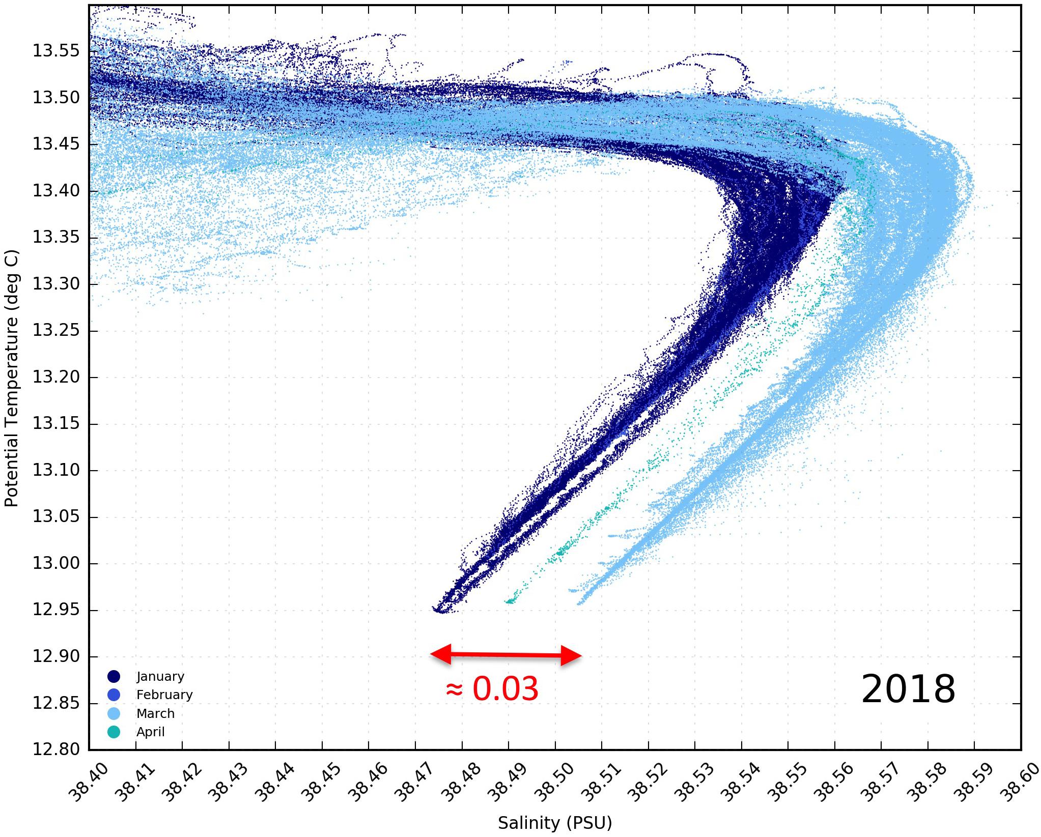
Figure 1. Deeper, more stable water, θ/S plot for four of the SOCIB Ibiza Channel monitoring line glider missions during 2018.

To achieve legacy value in historical observations, whether from gliders or any other observational platform, it is important that the typical magnitudes of large-scale global change are resolvable by the quality of the historical data over a sensible time frame. NOAA’s Geophysical Fluid Dynamics Laboratory has a blog presenting global surface salinity trends³ following Durack and Wijffels (2010), indicating that the largest long-term global changes in salinity that can be expected even at the ocean surface is around 0.004 psu per year.

Let us consider a trend of 0.003 psu per year, which is similar to that presented for stable waters of the western Mediterranean by Schroeder et al. (2016), and within the global maximum suggested above. If we add white noise to this trend, of maximum magnitude 0.030 psu, as would be suggested from Figure 1, then only over a sufficiently long period of at least 5–7 years can we expect any trend to be apparent, and even then apart from its direction, the trend is difficult to estimate with any degree of confidence (Figure 2). For the case shown in Figure 2, gradients and R² values were 0.0003, 0.0007; 0.0024, 0.0796; and 0.0028, 0.1598 for 3, 5, and 7 years, respectively.

FIGURE 2

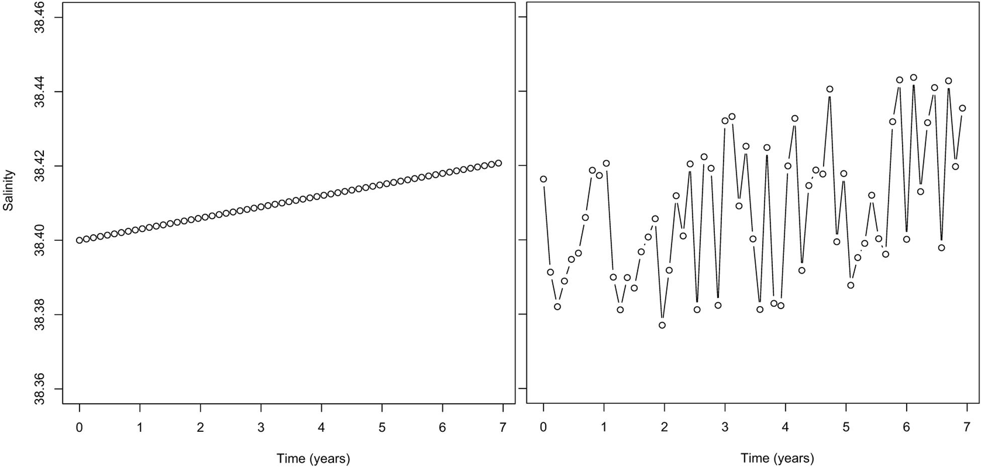
Figure 2. Seven years of a 0.003-psu modeled salinity trend beginning at 38.400 psu (left) and with the addition of white noise modeled measurement error of maximum magnitude 0.030 psu (right).

Cross-calibration and validation of CTD profile data are not new (Bosse et al., 2015). For many decades, since the introduction of the electronic CTD, oceanographers have compared their CTD data, normally in theta/salinity space as described in the next section, with historical profiles. This was to ensure that the short-term stability of well-studied known stable water masses, and mixing lines, were not compromised by subtle instrument and/or laboratory anomalies.

These comparisons traditionally involved overlaying profiles on a light box, or more often a window pane, to determine if differences were greater than acceptably small tolerances, often pushing manufacturers’ quoted tolerances to their limit and beyond. Taking a thoughtful step back from the science, in abstract, these highly learned oceanographers were in fact maximizing the overlap of plotted points in x–y space and therefore “maximizing whitespace” from an image analysis point of view.

A semi-automatic method for DM scientific field correction is presented in the following section. The tools presented in this manuscript are made freely available in accordance with Ocean Best Practice, and their URLs are given later. Our whitespace maximization technique was originally developed for the correction of thermal lag in towed vehicle CTD data, where the towed vehicles were being used for rapid environmental assessments by highly informed, but not necessarily expert, oceanographic teams for whom this might not always have been their primary task. This thermal lag application was only ever written up in unpublished documents by two of the authors. However, we mention this here as we hope that by the end of this manuscript, this and other potential future applications are clear and straightforward to implement.

Whitespace Maximization

Predominantly, glider vehicles use a SeaBird CTD instrument. SeaBird instrument laboratory calibrations are generally considered to set the industry standard, providing service intervals of typically 2 years are heeded. Nevertheless, the SeaBird technical manual accepts that an in-field calibration of conductivity to water bottle samples is desirable to approach and maintain a World Ocean Circulation Experiment (WOCE) standard of accuracy for salinity (King et al., 2001), historically quoted as 0.001–0.003 psu. Indeed, SeaBird will only quote their CTD instruments as capable of 0.003 psu, with a potential drift of 0.0003 psu per month.

The need for a temperature field correction is fairly unusual with SeaBird CTDs; however, the principle of correction is similar to that discussed in this section. If a temperature correction is thought to be necessary, then this should be applied first and salinity should be recalculated with the corrected temperature. The need for a conductivity field correction is common, typically manufacturers’ calibrations for salinity may be in error by the equivalent of a residual salinity offset up to the ±0.010 psu level, depending on the laboratory service/calibration history of the CTD instrument, as described earlier and above. It is not that unusual to find real-time glider data with an inaccurate calibration such that salinity can exhibit an apparent residual of 0.030 at salinities of ∼38.500 as shown in Figure 1 earlier, and in the SOCIB’s experience, considerably higher than this is possible.

Field correction of lowered CTD data is traditionally achieved with coincident collection of water bottle samples and subsequent laboratory analyses. However, unlike the traditional CTD frame, glider vehicles have no facility for taking discrete water samples for careful laboratory analysis. Of course, this problem is not new; towed undulating vehicles (Allen et al., 2002) and moorings have been used to carry CTD instruments for many years and generally these too suffered from the limitation of lack of water bottle sampling for in situ correction. Field correction in these cases has to take the form of an inter-calibration process with other known and trusted datasets for particularly constant or only very slowly varying characteristic water types and water masses. Now that multi-platform observations are more common, it is essential that corrections through inter-calibration procedures are routinely included in the DM data processing. Any salinity or temperature comparisons between datasets should always be made by plotting potential temperature against salinity on a θ/S diagram, as this is the best way to identify key characteristic water types in the vertical structure of the water; it overcomes the fact that both temporally and geographically, characteristic water types can be found at significantly different depths in the water column, which can vary significantly on short timescales due to processes such as Internal Waves and the propagation of eddies.

For gliders, a semi-automatic inter-calibration methodology has been developed by SOCIB to field correct its glider data, both for regular monitoring lines and for specific process study programs. The methodology is based around the identification and use of characteristic stable structures in potential temperature/salinity (θ/S) diagrams from well-calibrated lowered CTD data. The most contemporary (in space and time) DM corrected research cruise CTD datasets are chosen to match with Glider mission datasets. For SOCIB monitoring lines such as that across the Ibiza and Mallorca channels, this is generally quite straightforward as short (3-day) seasonal research vessel cruises are carried out to enable a laboratory analysis constraint for the quality of the semi-continuous glider monitoring. More disparate glider missions for process studies require more manual intervention in the selection of well-calibrated CTD reference data. In both cases, however, particular turning points (water types) and mixing lines (water masses), in the θ/S diagrams, are compared to identify the difference between the uncorrected glider data and the water bottle corrected ship CTD data.

We appreciate that some facilities, laboratories, and operators may not have access to their own reference bottle calibrated lowered CTD datasets. In this case, local, national, or international databases may need to be relied upon. Good databases will have levels of confidence or accuracy to the quality of the calibrated data provided in their metadata. Ideally, the vertical resolution of the reference datasets should be approximately the same as or better than the glider data, i.e., ∼1 m or 1 db, or better. Again, most good databases should be able to supply this. Lower vertical resolution will have some limiting effect on the quality of the final result, although interpolation of the data and/or increasing the dot size in the θ/S diagrams (described later) may afford an acceptable cross-calibration.

Shallow glider data and shallow water applications for glider platforms may be unsuitable for DM inter-calibration as presented in this paper. Stable and well-defined water masses and mixing lines are not common in near-surface or shallow waters, where high-frequency air–sea interaction processes can effect water temperature changes and freshwater input independently and lead to considerable variability in θ/S space. For these applications, the operator may not be able to do better than accept the error in manufacturer’s instrument calibration and instrument drift, unless they have access to their own calibration facilities or a mechanism for taking bottle samples very close to the glider vehicle.

As recommended in SeaBird, Application Note 31, for their CTD instruments, the glider salinity values are corrected as a conductivity slope⁴ (AN-31), Eq. 1, where A is the conductivity correction coefficient. It is worth noting that in ocean regions where salinity and temperature ranges are small, an offset correction can provide equivalent results.

$$Conductivity\mathrm{\_}corrected\text{=}A*Conductivity\mathrm{\_}measured(1)$$

Generally, the slope correction is iteratively determined (Figure 3), as required to get a good overlap between glider and ship datasets on the θ/S diagram. A semi-automated procedure of maximizing whitespace in overplotted corrected CTD and glider θ/S data has been developed. This involves the creation of a θ/S diagram of “background” ship data, and “test” glider data. The whitespace maximization is then carried out, whereby the test data are iteratively moved along the x (salinity) axis by changing the value of coefficient A in Eq. 1, and a calculation of the whitespace area, i.e., the number of empty or white pixels, in the θ/S diagram figure is carried out. The iterative procedure continues to adjust the conductivity correction coefficient (i.e., the coefficient that ultimately leads the shift in the test data to the left or right) until the whitespace area of the figure has reached a maximum. This occurs when the test data are most closely overlying the background data. Confidence in the glider salinity values is then typically better than 0.010 psu (Figure 4) assuming a normal confidence in ship CTD-calibrated datasets of better than 0.003 psu.

FIGURE 3

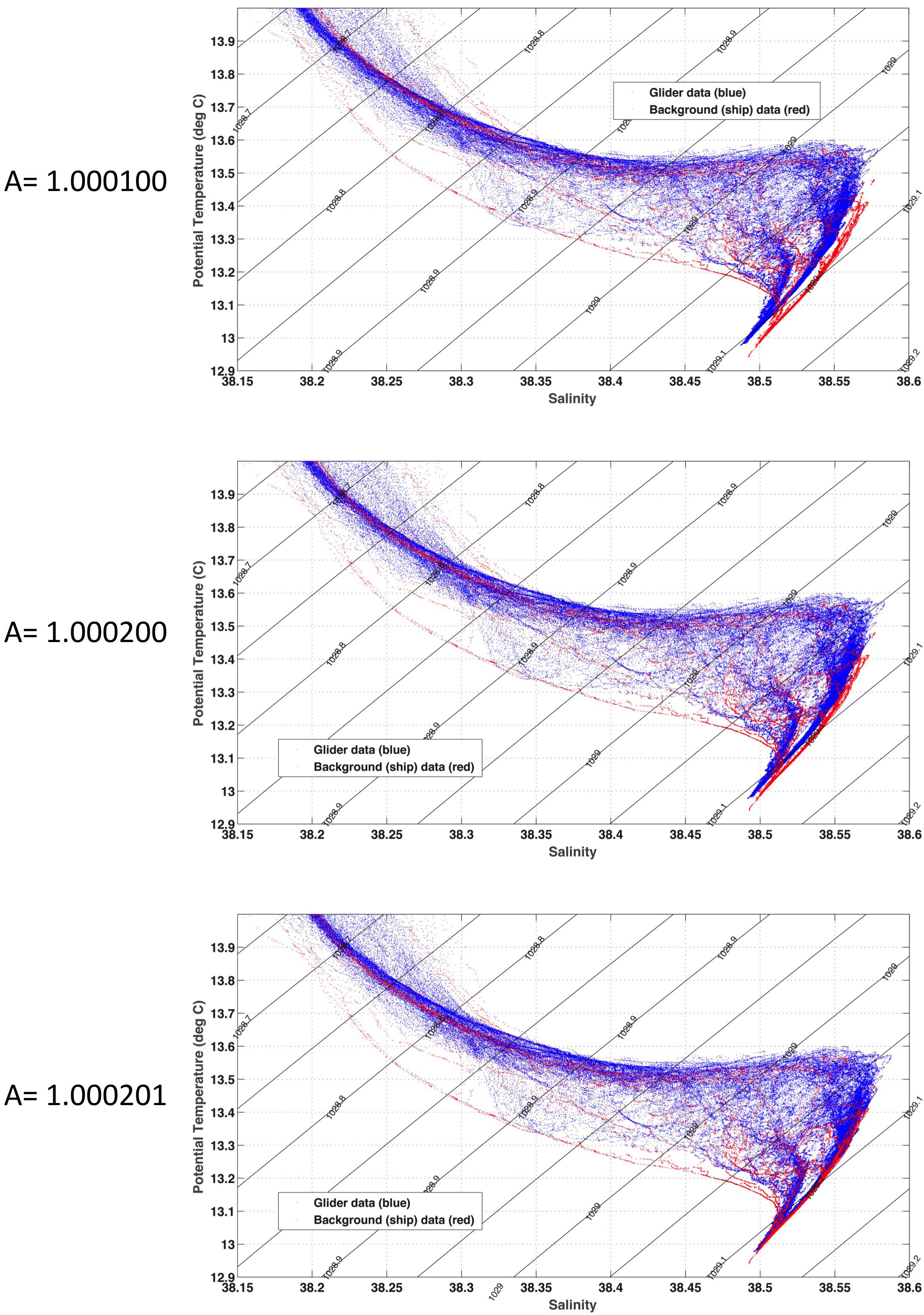
Figure 3. The iterative selection of gradient A, when field correcting glider data to CTD stations.

FIGURE 4

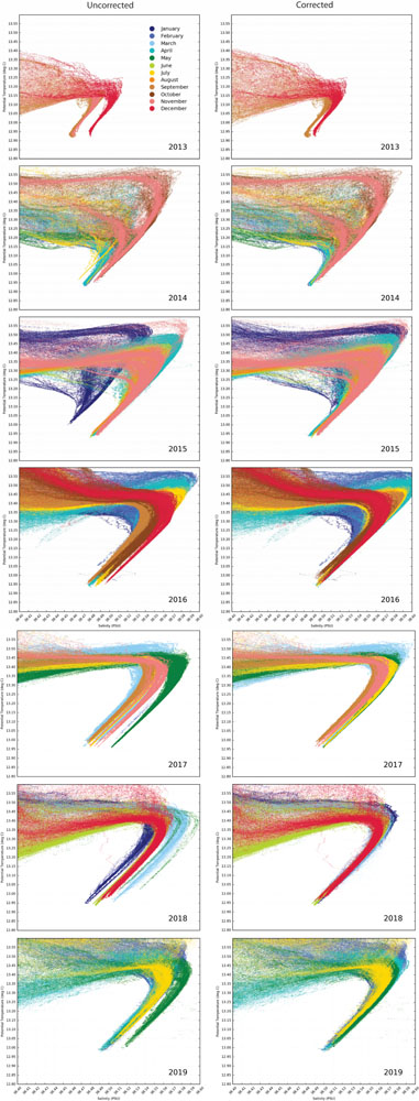
Figure 4. θ/S diagrams zoomed in to show the relatively stable intermediate water mixing line between Levantine Intermediate Water and Western Mediterranean Deep Water for SOCIB glider missions across the Ibiza and Mallorca Channels separated into years from September 2013 to July 2019. On the left are the uncorrected glider profiles, and on the right are the DM field corrected glider profiles (x-axis tick mark interval is 0.010). These data and the relevant CTD datasets are available through the SOCIB Data Centre website (www.socib.es/?seccion=dataCenter).

The inter-calibration correction procedure is only semi-automatic because preparation for the whitespace maximization may require several subjective expert decisions, described later, which may influence the outcome of the automated correction. The appropriate background reference data need to be used, where ideally both spatial and temporal separation of the datasets should be as small as possible. If the most contemporary DM corrected research cruise CTD datasets and the glider CTD dataset are not quasi-synchronous, a difference in time of more than a few weeks, for example, the glider θ/S diagrams are then analyzed from a climatic point of view by paying attention to the seasonal evolution during that year (corrected glider and ship missions before and after the glider mission) and to the inter-annual evolution (corrected ship and glider missions from a similar seasonal time period in previous years). Any inter-annual evolution must of course bear in mind the possibilities of long-term water mass changes and decadal scale variability.

At SOCIB, we have created a further GUI stage to request the user preferred method of comparing with cruise datasets from our database, with the following options:

Manual selection of specific cruises

All Cruises of a particular monitoring program

All Cruises of the same season

All Cruises of the same season and cruises directly before and after

Matching Cruise (if one exists) and cruises directly before and after.

The results of choosing different options can be compared to investigate the sensitivity to seasonal and interannual variability. The matter of allowing for interannual variability is of great importance as it is becoming increasingly well observed that there may be an increasing salinity trend in intermediate waters of the Mediterranean (Schroeder et al., 2016).

In Figure 4, if we focus on the mean salinity for every glider mission, between 12.90 and 13.00 potential temperature (°C), we can look for long-term trends and variability in this important mixing line in the Western Mediterranean. The actual oceanography presented here is not the subject of this manuscript; it is being prepared for submission in a separate manuscript; however, here we want to show how important the DM field correction is to establishing both short-term variability and long-term trends. To this end, in Figure 5, we present the mean salinity between θ = 12.90 and 13.00; we can see that the uncorrected data (blue triangles) are very noisy around the calculated trend line (blue), with a residual standard deviation of 0.004 salinity and maximum residual of 0.018. The DM field corrected data (red circles) are much cleaner around the trend line (red) with a residual standard deviation of 0.002 salinity and a maximum residual of 0.008. The uncorrected data suggest a long-term salinity trend of +0.005 salinity/year. The DM field corrected data suggest a long-term trend of +0.002 salinity/year. However, the much reduced noise level in the corrected data allows us to see more detail, and although the overall 6-year trend may be 0.002 salinity/year, the dotted green lines suggest a steeper trend, around 0.003 salinity/year, until August 2017 and a further trend of around 0.006 salinity/year for the latest 2 years. As pointed out earlier, the subject of what may have happened in the middle of 2017, from an oceanography perspective, is beyond the scope of this manuscript.

FIGURE 5

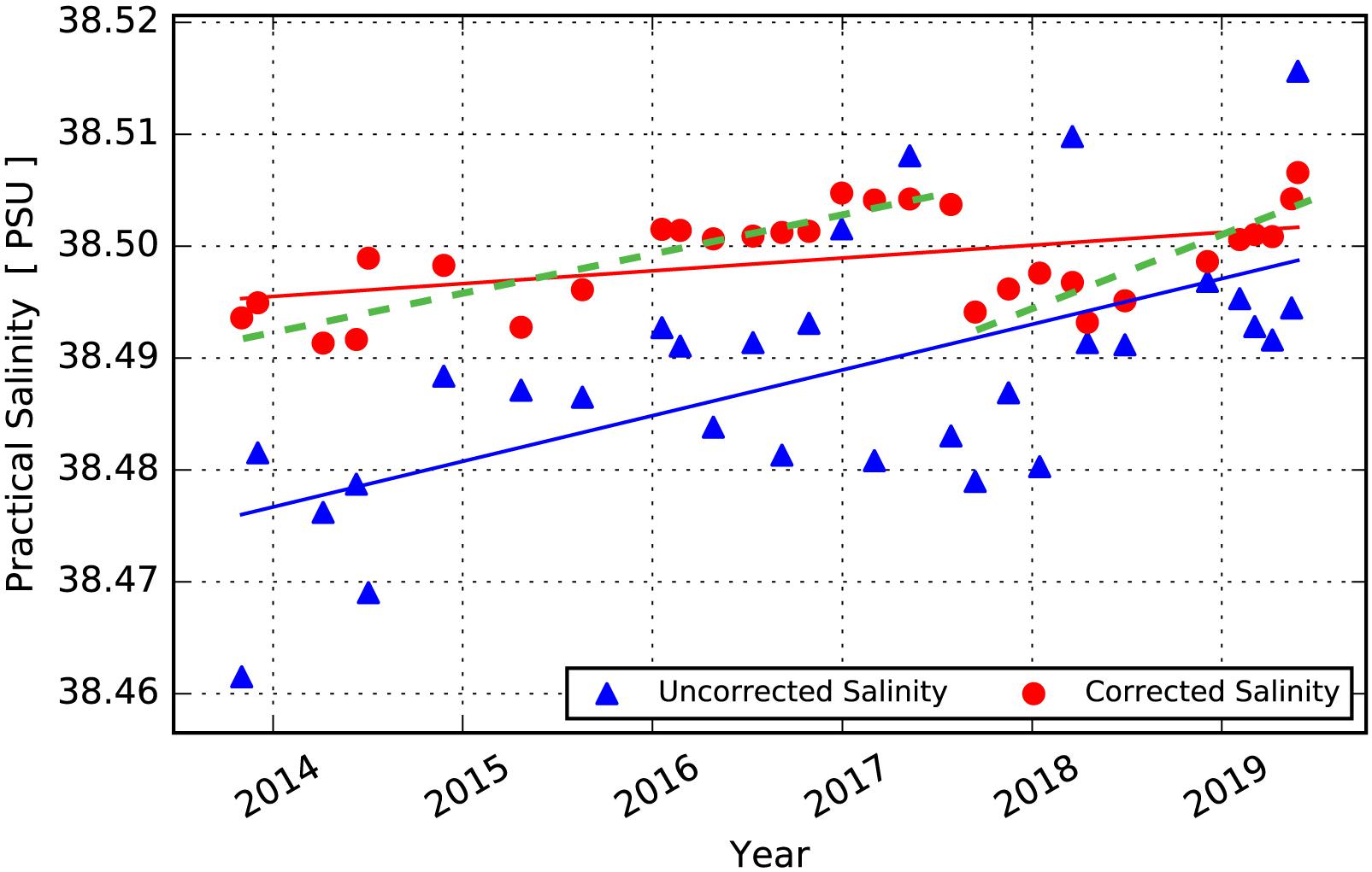
Figure 5. Mean salinity between potential temperatures 12.90 and 13.00 (°C) for each glider mission, for uncorrected glider data (blue), and DM field corrected glider data (red).

The axes used in the θ/S diagrams need to be appropriate for the inter-calibration correction (e.g., Figure 3), for example, excluding highly variable surface data, and avoiding water column regions where the background data points are populated with a wide natural variability in salinity. In other words, the region of θ/S diagram space predominantly used for inter-calibration correction purposes should focus on the most stable parts of the water column; while a significant range in salinities overall is required for a reliable correction, this will generally be where the variation in salinity with any given temperature is low, and thus the data points densely overlay each other. This typically describes mode water types, well-defined mixing lines, and water masses, in intermediate and deeper waters. It should be noted that horizontal (vertical) mixing lines in the theta-S diagram will not provide much information to fit salinity (temperature) and preference should be given to mixing lines with some variation in temperature (salinity).

SOCIB has created a Glider salinity correction pack (Figure 6) written in MATLAB and Python; it is available through GitHub at github.com/socib/salinity-correction-toolbox and has the DOI, 10.5281/zenodo.354169; the user manual can be found at repository.socib.es/repository/entry/show?entryid=74d6c56a-0c87-4790-8e0b-5896b540557c and its contribution to Ocean Best Practices is provided at repository.oceanbestpractices.org/handle/11329/459. The Glider salinity correction pack has four phases. In the first phase, user input is required to determine which lowered CTD and Glider datasets are to be processed, what axis limits to use for the comparison θ/S diagrams, and which data are on the topmost layer of the diagram (and are thus most visible). The user is advised to create a plot of all background ship CTD data and the glider data to allow for a sensible decision on which background ship data should be used, first for the whole axis range and then for a “zoomed in” θ/S diagram. The user can of course re-run segments of the code if they are not satisfied with the decisions they have made. In a second stage, the automatic whitespace maximization procedure requires user input to decide on the axis limits, and create θ/S diagrams of the background and glider data to check whether the user is happy with the decisions made (Figure 3).

FIGURE 6

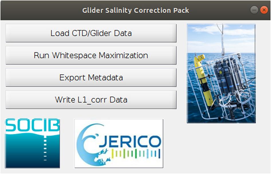
Figure 6. The MATLAB GUI for the SOCIB Glider salinity correction pack.

By default, the automatic whitespace iteration procedure is carried out three times with different initial guesses for the correction coefficient, A, in Eq. 1. One of these guesses should always be 1 (i.e., no initial movement of the glider data). For the other two initial guesses, the user is advised to use guesses that move the glider data to the left and to the right of the background data to begin with. SOCIB’s software uses by default, A = 0.9999, 1.0000, and 1.0001 as the three initial guesses; this is equivalent to offsets of ±0.004 in salinity at Mediterranean water salinities of 38.500; in more characteristic Atlantic waters, these initial guesses would be equivalent to offsets of ±0.003. The iteration procedure has three step levels, major steps of 0.0001, minor steps of 0.00001, and miniscule steps of 0.000001, with equivalent offsets of 0.004, 0.0004, and 0.00004, respectively, at 38.500 salinity. Each of the three starting scenarios (Figure 7) begins by moving in major steps to the left (lower salinity) or right (higher salinity), testing the whitespace pixel count each time, and the steps then continue in the most whitespace increasing direction until the whitespace begins to decrease. At this point, the program changes to the minor step level and reverses direction until the whitespace stops increasing and this same procedure is then repeated with miniscule steps.

FIGURE 7

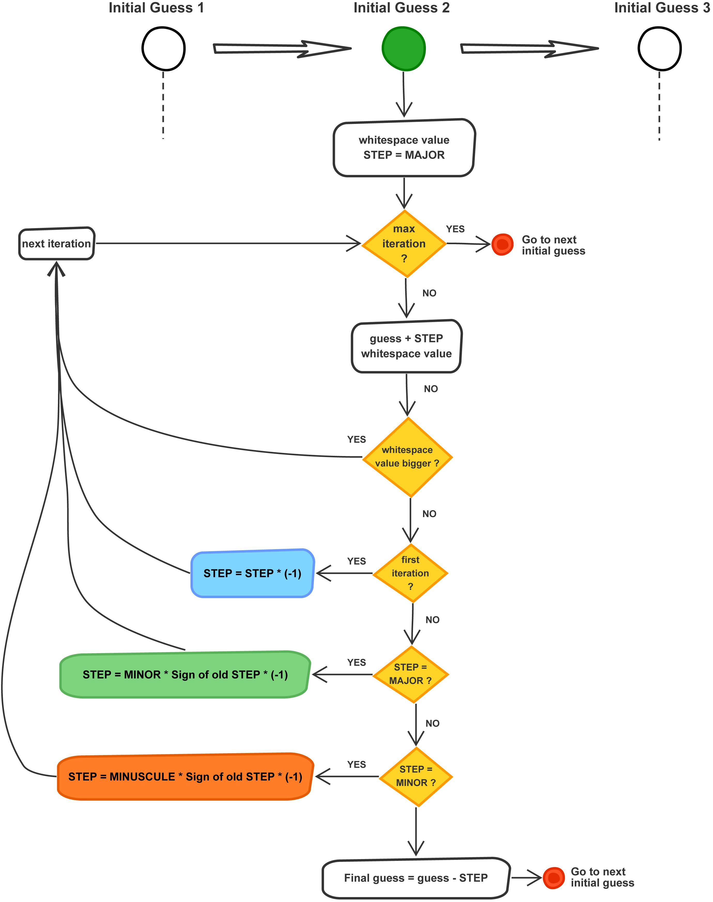
Figure 7. Flow diagram for the whitespace maximization component of the SOCIB glider salinity DM scientific correction toolbox. For the sake of brevity, only the second initial guess procedure is shown as all initial guess procedures are the same.

θ/S diagrams of the corrected glider data over the background data for all three scenarios are created and the user is then asked to select their preferred scenario solution in the case of there being more than one solution. The user is also asked to estimate the error, which can be done simply by looking at the thickness of the “thinnest” segment of the final θ/S diagram and estimating the range of salinity values the glider data could effectively have taken; however, the user may have other preferences for estimating error.

Finally, in the third and fourth stages, final θ/S diagrams showing background data, and uncorrected and corrected glider data are created, with user-defined axis limits, and a summary file is created detailing the correction coefficient, error estimate, standard deviation of the corrected CTD background data, and a summary of the correction procedure and correction reference dataset; this summary information enters the metadata, for the field corrected data file.

As we mentioned earlier, the semi-automatic whitespace maximization was originally developed for simple linear thermal lag correction:

$$T_{\text{C}}\text{=}{T}_{\text{M}}+(\mathrm{\tau }.\mathrm{\Delta }T),(2)$$

where T_C is the corrected temperature, T_M is the measured temperature, ΔT is the difference in temperature over an instrument sampling interval, and τ is the best solution time constant. In this case, the adjustment generally moves in just one direction toward increasing τ, until the final small adjustments to determine the optimal time constant for cleaning up a noisy θ/S profile for example. In the case of field correction presented here, A in Eq. 1 could be more than 1 or less than 1, and depending on the initial guess, the data point dot size, and the choice of parameter ranges over which the whitespace maximization is to be carried out, the simplest maximization could be just to move the datapoints successively off the plot page. While the choice of three initial guesses, and the choice of parameter ranges is made interactively through the GUI (Figure 6), the data point size is normally more generic and therefore currently requires a lower level change of point size value in the toolbox code. The dot size can be set by the user in line 58 (markerSize = 10), of function imageArea_V2.m, as shown in Figure 8. It was set to 10 points based on our experience inter-calibrating the 7 years of datasets shown earlier. Simple modification of the main code could also allow the user to directly set the marker size through the User Interface; however, we doubt if this would be required frequently enough to make this worthwhile.

FIGURE 8

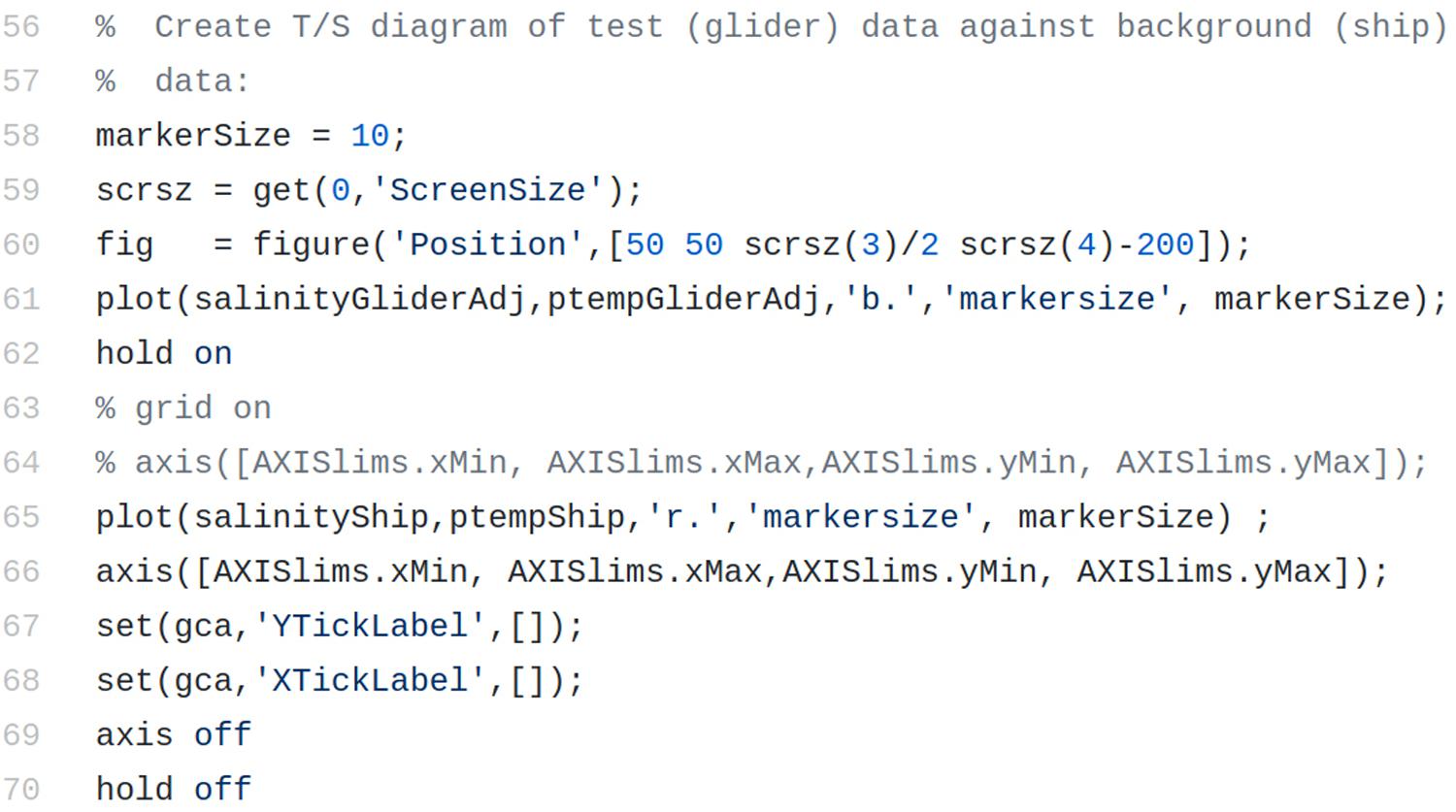
Figure 8. Section of function imageArea_V2.m, indicating where, on line 58, the plotted dot size may be changed (markerSize = 10).

Occasionally, there may be more than one subtly different flavor of stable mixing line during a single glider mission, which can last up to 2 months or more; this is identified by having more than one solution from the three initial guesses as mentioned above. Much of the time, the resulting uncertainty is within the 0.003 level that the manufacturer would set as limiting anyway and we can select any one of the solutions. However, it can indicate that the glider dataset needs to be split before inter-calibration, either due to a change in instrument characteristics, or, rarely, that a genuine subtle change in mixing line has occurred during a glider mission. The latter can only be fully confirmed by a similar subtle change in mixing line between bottle calibrated CTD data before and after the glider mission. On these relatively rare occasions, more comparison of the shape of the overall θ/S profile in the shipboard lowered CTD and glider datasets may be required to identify which mixing line should be matched to the CTD dataset, or whether more than one shipboard lowered CTD dataset needs to be combined to incorporate the subtle change in mixing line.

Delayed Mode Metadata

A detailed history of ship and glider slope change values is kept on record from mission to mission. It is important to keep in mind that conductivity sensors tend to drift with time rather than jump about in their calibration correction, although jumps are not unknown. Generally, SeaBird is correct in its assertion that conductivity correction will simply take the form of a gradient operator, i.e., Eq. 1. However, it should be considered possible that offsets or even higher order operators may be necessary if an instrument is significantly out of calibration

$$Conductivity\mathrm{\_}corrected\text{=}B+(A*Conductivity\mathrm{\_}measured)(3)$$

or

$$Conductivity\mathrm{\_}corrected\text{=}B+(A*Conductivity\mathrm{\_}measured)$$

$$\mathrm{\hspace{1em}}+(C*{(measuredconductivity)}^2);(4)$$

although we have not yet experienced either of these at SOCIB. However, the method for inter-calibration would follow the same procedures just with Eqs 3 or 4 instead of Eq. 2.

How to distribute DM calibrated glider data is the final problem to address. What information is required in the metadata files is a question still to be fully answered by the glider community, but it is necessary to keep a cross reference to the dataset used for the glider correction. We suggest, at a minimum, that the following information about the chosen reference dataset should be carried with the corrected glider dataset global attributes, which will enable users to interpret and cross check the resultant corrections at any time in the future if required: instrument type (e.g., CTD, manufacturer, and serial number), mission, platform, time, geographical coordinates, and explanatory comments. SOCIB also includes correction coefficient, confidence level (residual error estimate), standard deviation of the corrected CTD background data, and a summary of the correction procedure and correction reference dataset, in the final metadata for the corrected variables (Figures 9, 10). SOCIB is closely supportive of both EGO and JCOMMOPS in helping to refine international standards for metadata and DM Quality Control.

FIGURE 9

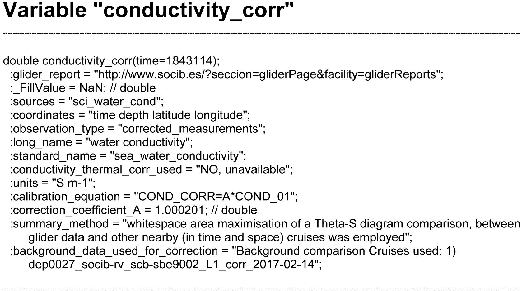
Figure 9. An example of the Metadata that accompany the DM scientific corrected conductivity data in SOCIB’s Data Centre.

FIGURE 10

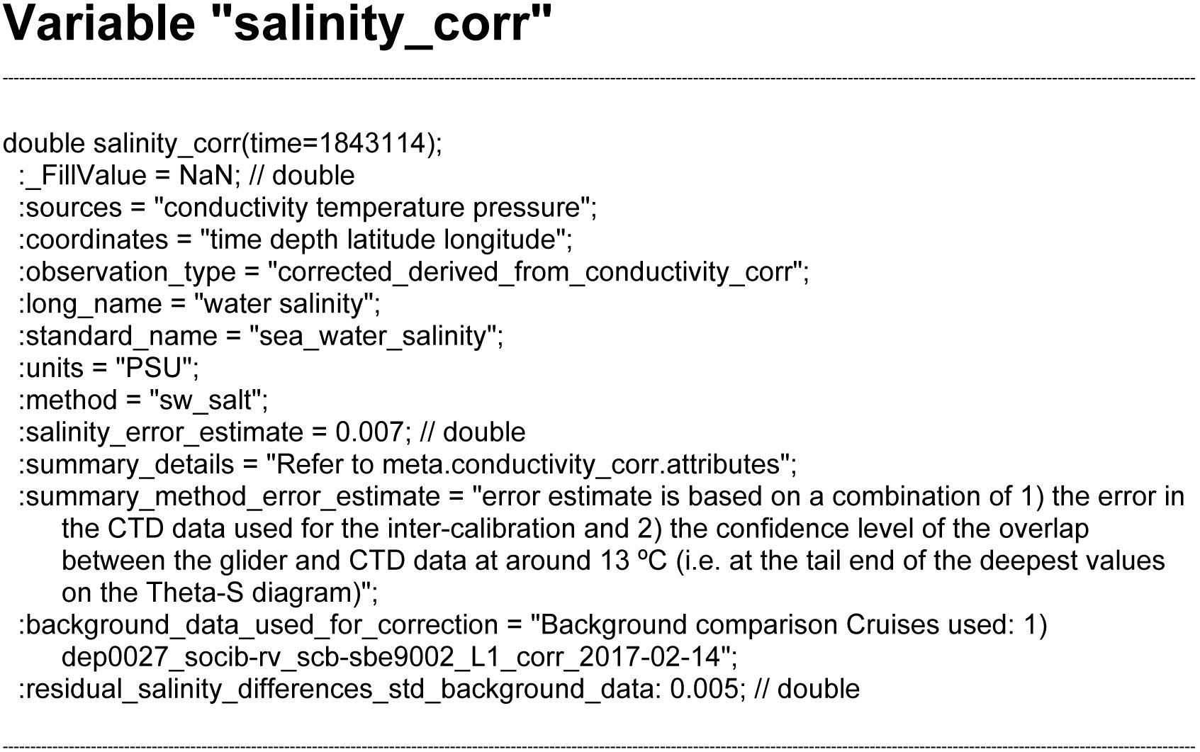
Figure 10. An example of the Metadata that accompany the DM derived salinity data in SOCIB’s Data Centre.

The new metadata variables added for the DM corrected conductivity and salinity variables, “Conductivity_corr” and “Salinity_corr”, respectively, are as follows:

Conductivity_corr:calibration_equation: The equation used to correct conductivity in DM.correction_coefficient: The determined value of the DM correction coefficients.summary_method: A description of the method used to find the DM correction coefficients.background_data_used_for_correction: A description of the reference datasets used for DM correction.

Salinity_corr:salinity_error_estimate: The estimated confidence level for the DM corrected salinity.summary_details: A reference to the method used—normally to the conductivity metadata.summary_method_error_estimate: A description of how this confidence level was derived.background_data_used_for_correction: A description of the reference datasets used for DM correction—normally duplicated from the conductivity metadata.residual_salinity_differences_std_background_data: The estimated confidence level for the DM reference datasets—copied from the metadata for the reference datasets.

Conclusion and Future

The effort afforded by the oceanographic community to monitor the oceans has accelerated significantly since first the introduction of the Argo float and more recently the adoption of glider vehicles. The increased realization that ocean monitoring is critical to understanding climate and global change processes was probably instrumental in driving the new technologies, and it certainly is critically dependent on them. The availability of ocean data over the past 10–20 years has grown exponentially and the quality control of these data is of crucial importance.

The presentation of scientific inter-calibration correction procedures for DM glider salinity data collection, as given in this paper, has clear links with the field correction of biogeochemical parameters. Comparison between dissolved oxygen measurements using a CTD mounted SeaBird Electronics SBE 43 oxygen instrument, calibrated to Winkler titration determined oxygen concentration (Langdon, 2010) of in situ water samples, and oxygen concentration determined from glider mounted Aanderaa optodes is a natural extension of the work presented here and has begun in many laboratories including SOCIB. In Figure 11, we clearly see that an offset and amplification procedure such as can be applied by Eq 3 or 4 is needed to pull the glider data (blue) into line with the CTD datasets on both a θ/oxygen diagram (shown) and a salinity/oxygen diagram (not shown). In at least this respect, SOCIB also has ambitions to develop the toolbox further in the field of machine learning. In this example, in just the same way as the authors and readers can easily identify the type of equation requiring application to the blue data in Figure 11, in order to maximize whitespace by shape recognition, there exist expert shape recognition algorithms that can be incorporated into future versions of the toolbox to enable machine algorithm choice, and perhaps later even machine algorithm design, to automate the field correction procedure further.

FIGURE 11

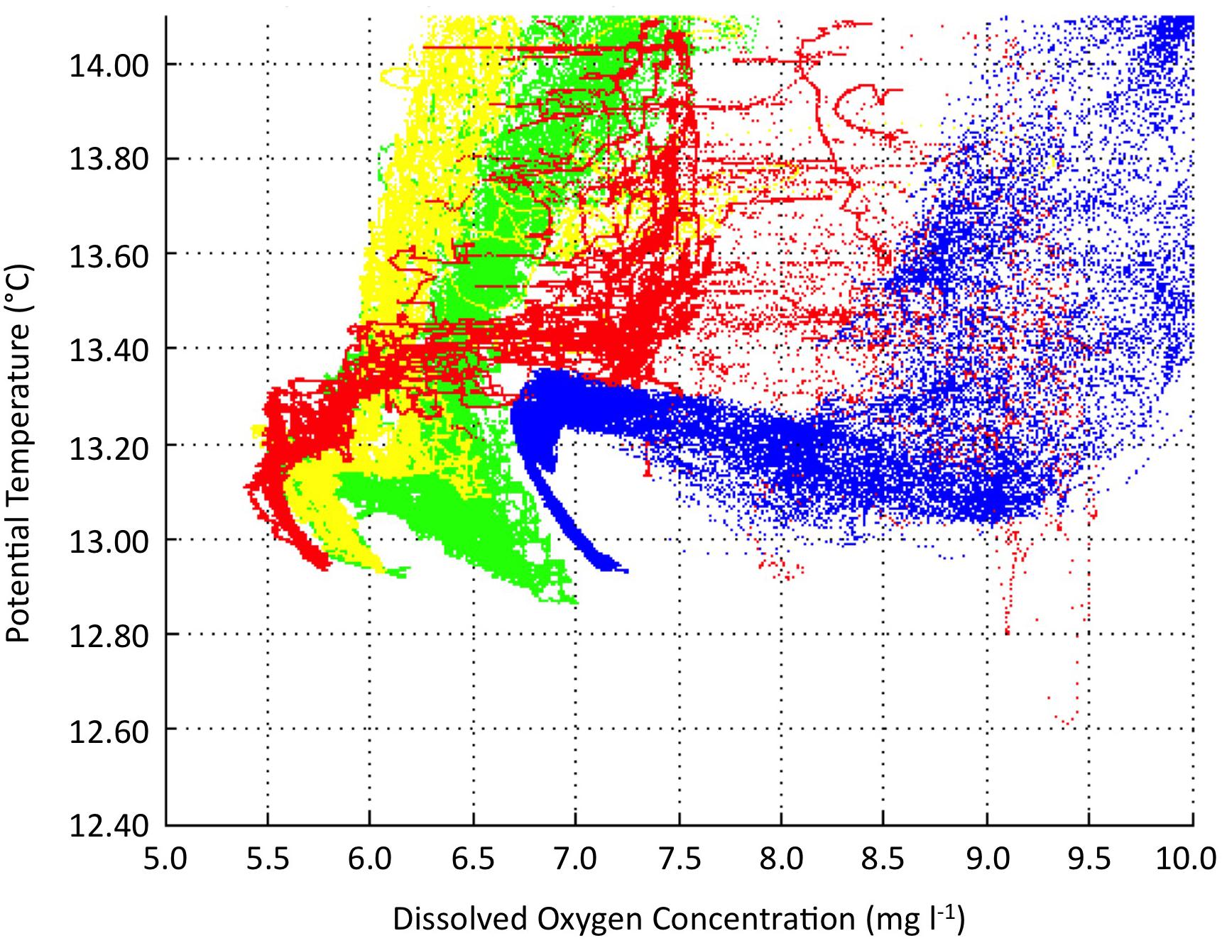
Figure 11. A potential temperature/oxygen (θ/O) diagram, showing the typical size of correction necessary for DM field correction of a glider mission (blue) to bottle calibrated ship CTD survey data (red, yellow, green).

Similarly, cross-calibration correction of glider mounted fluorometers and optical backscatter sensors is the subject for further expansion of the work presented here, although we take careful note that these two types of biomass measurement are very dependent not only on environmental variables (such as irradiance) but also on the community species composition of the in situ plankton. These are subjects that will develop significant links between work in progress on the integration of biological data, with the enhancement of quality control procedures for sensor-based biogeochemical data.

The procedures developed are focused on adopting, promoting, and developing internationally agreed standards for the quality control and inter-calibration of ocean observing networks. This is critical to understanding long-term changes in the ocean environment, particularly as the length of the observing history is short compared to the expected timescale of the global and climate changes taking place. SOCIB’s work is therefore highly relevant to our interactions with European and international ocean observing networks. In addition, our support of international standards and their development are a key component of the JERICO label as developed under JERICO, JERICO NEXT, and the recently funded JERICO S3 EU programs. The reliability of an observing network, as judged by its ability to deliver world-class useable information, depends most of all on methodical calibration and assessment activities. The four-dimensional characterization of trans-boundary hydrography and transport will need to be fed with world-class inter-calibrated and quality-controlled data to complete a chain of implicit and explicit collaboration.

Data Availability Statement

The datasets generated for this study are available on request to the corresponding author.

Author Contributions

JA and JG contributed to conception and original code design. JA and CM contributed to Whitespace code writing and data correction. CM and KR contributed to Toolbox design and coding. JA contributed to manuscript planning. JA, CM, and EA-F contributed to manuscript writing, preparation of figures, and submission steps. EA-F, KR, NZ, and JG contributed to manuscript proofreading. All authors approved the final version of the manuscript.

Funding

This work was partially supported by the JERICO-NEXT funded by the H2020 Framework Program, under grant agreement No. 654410.

Conflict of Interest

JG was employed by Valeport Ltd.

The remaining authors declare that the research was conducted in the absence of any commercial or financial relationships that could be construed as a potential conflict of interest.

Acknowledgments

We thank the SOCIB Glider Facility, the R/V SOCIB crew, the SOCIB Data Centre Facility, and the SOCIB Engineering and Technology Development Division, without whom none of these data could have been collected. We thank Andrea Cabornero for assistance in the field and the laboratory and Irene Lizarán for excellent salinity analysis. Finally, we are indebted to the reviewers and editors for their support, comments, and suggestions.

Footnotes

1. ^ https://github.com/socib/glider_toolbox
2. ^ www.byqueste.com/toolbox.html
3. ^ www.gfdl.noaa.gov/blog_held/14-surface-salinity-trends/
4. ^ www.seabird.com/application-notes

References

Allen, J., Dunning, J., Cornell, V., Moore, M., and Crisp, N. (2002). Operational oceanography using the ‘new’ SeaSoar ocean undulator. Sea Technol. 43, 35–40.

Google Scholar

Baumgartner, M. F., Stafford, K. M., Winsor, P., Statscewich, H., and Fratantoni, D. M. (2014). Glider-based passive acoustic monitoring in the arctic. Mar. Technol. Soc. J. 48, 40–51. doi: 10.4031/mtsj.48.5.2

CrossRef Full Text | Google Scholar

Bosse, A., Testor, P., Mortier, L., Prieur, L., Taillandier, V., d’Ortenzio, F., et al. (2015). Spreading of levantine intermediate waters by submesoscale coherent vortices in the northwestern Mediterranean Sea as observed with gliders. J. Geophys. Res. Oceans 120, 1599–1622. doi: 10.1002/2014jc010263

CrossRef Full Text | Google Scholar

Durack, P., and Wijffels, S. (2010). Fifty-year trends in global ocean salinities and their relationship to broadscale warming. J. Clim. 23, 4342–4362. doi: 10.1175/2010JCLI3377.1

CrossRef Full Text | Google Scholar

EGO Gliders Data Management Team (2017). EGO Gliders NetCDF Format Reference Manual, eds T. Carval, C. Gourcuff, J.-P. Rannou, J. J. H. Buck, and B. Garau, Paris: Ifremer. doi: 10.13155/34980

CrossRef Full Text | Google Scholar

Fer, I., Peterson, A. K., and Ullgren, J. (2014). Microstructure measurements from an underwater glider in the turbulent faroe bank channel overflow. J. Atmos. Oceanic Technol. 31, 1128–1150. doi: 10.1175/JTECH-D-13-00221.1

CrossRef Full Text | Google Scholar

Gregor, L., Ryan-Keogh, T. J., Nicholson, S.-A., du Plessis, M., Giddy, I., and Swart, S. (2019). GliderTools: a python toolbox for processing underwater glider data. Front. Mar. Sci. 6:738. doi: 10.3389/fmars.2019.00738

CrossRef Full Text | Google Scholar

King, B. A., Firing, E., and Joyce, T. M. (2001). “Chapter 3.1 Shipboard observations during WOCE,” in International Geophysics, Vol. 77, eds G. Siedler, J. Church, and J. Gould (Cambridge, MA: Academic Press), 99–122. doi: 10.1016/S0074-6142(01)80114-5

CrossRef Full Text | Google Scholar

Langdon, C. (2010). “Determination of dissolved oxygen in seawater by Winkler titration using the amperometric technique,” in GO_SHIP Repeat Hydrography Manual: A Collection of Expert Reports and Guidelines, eds B. M. Sloyan and C. Sabine (Paris: IOC/IOCCP).

Google Scholar

Owens, W. B., and Wong, A. P. S. (2009). An improved calibration method for the drift of the conductivity sensor on autonomous CTD profiling floats by theta-S climatology. Deep Sea Res. Part I Oceanogr. Res. Pap. 56, 450–457. doi: 10.1016/j.dsr.2008.09.008

CrossRef Full Text | Google Scholar

Schroeder, K., Chiggiato, J., Bryden, H. L., Borghini, M., and Ben Ismail, S. (2016). Abrupt climate shift in the Western Mediterranean Sea. Sci. Rep. 6:23009. doi: 10.1038/srep23009

PubMed Abstract | CrossRef Full Text | Google Scholar

Testor, P., de Young, B., Rudnick, D. L., Glenn, S., Hayes, D., Lee, C. M., et al. (2019). OceanGliders: a component of the integrated GOOS. Front. Mar. Sci. 6:422. doi: 10.3389/fmars.2019.00422

CrossRef Full Text | Google Scholar

Thomsen, S., Karstensen, J., Kiko, R., Krahmann, G., Dengler, M., and Engel, A. (2019). Remote and local drivers of oxygen and nitrate variability in the shallow oxygen minimum zone off Mauritania in June 2014. Biogeosciences 16, 979–998. doi: 10.5194/bg-16-979-2019

CrossRef Full Text | Google Scholar

Tintoré, J., Perivoliotis, L., Heslop, E., Poulain, P. M., Crise, A., and Mortier, L. (2015). “Strategy for an integrated ocean observing system in the Mediterranean and Black Seas (Recommendations for European long term sustained observations in the SES),” in PERSEUS Project, (New York, NY: PERSEUS).

Google Scholar

Tintoré, J., Vizoso, G., Casas, B., and Heslop, E. (2013). SOCIB: the Balearic islands observing and forecasting system responding to science, technology and society needs. Mar. Tech. Soc. J. 47, 17. doi: 10.4031/MTSJ.47.1.10

CrossRef Full Text | Google Scholar

Todd, R. E., Rudnick, D. L., Sherman, J. T., Owens, W. B., and George, L. (2017). Absolute velocity estimates from autonomous underwater gliders equipped with doppler current profilers. J. Atmos. Oceanic Technol. 34, 309–333. doi: 10.1175/JTECH-D-16-0156.1

CrossRef Full Text | Google Scholar

Troupin, C., Beltran, J. P., Heslop, E., Torner, M., Palmer, M., Garau, B., et al. (2015). A toolbox for glider data processing and management. Methods Oceanogr. 13–14, 13–23. doi: 10.1016/j.mio.2016.01.001

CrossRef Full Text | Google Scholar

Wong, A. P. S., Johnson, G. C., and Owens, W. B. (2003). Delayed-mode calibration of autonomous ctd profiling float salinity data by θ/S climatology. J. Atmos. Oceanic Technol. 20, 308–318. doi: 10.1175/1520-0426(2003)020<0308:dmcoac>2.0.co;2

CrossRef Full Text | Google Scholar