Seasonal Distribution of Tuna and Non-tuna Species Associated With Drifting Fish Aggregating Devices (DFADs) in the Western Indian Ocean Using Fishery-Independent Data

Introduction

Pelagic ecosystems are highly dynamic environments in time and space (Kaplan et al., 2010; Dueri and Maury, 2013), accounting for 99% of the biosphere volume (Angel, 1993) and supplying more than 80% of the fish consumed by humans (Pauly et al., 2002). Due to the limited knowledge of pelagic ecosystem functioning and diversity (Kaplan et al., 2014), there is an increasing need to obtain reliable spatial information on pelagic species distributions (Costello and Kaffine, 2010). Indeed, it is necessary to understand how marine populations are distributed across the environment, and the drivers of their movement and dynamics, for a correct assessment of fish populations and ecosystem functioning, and, hence, fisheries management and conservation of exploited species (Paradinas, 2017).

The industrial tropical tuna purse seine fishery is one of the most important fisheries in the world, accounting for 64% of tuna catches worldwide (ISSF, 2019). In the Indian Ocean, more than 80% of the total sets of purse seiners in recent years have been on man-made drifting fish aggregating devices (DFADs) (Báez et al., 2018). The remainder of the purse seine fishery catch comes from sets on unassociated tuna schools, also known as free-swimming schools. In the past, the majority of floating objects used by fishers were natural floating objects (e.g., driftwood, logs or coconuts) encountered by chance, traditionally called “logs.” Over time, the objects were modified by fishers and, thus, an operational definition was adopted for them (i.e., man-made DFADs) to separate them from natural floating objects. Because of the aggregative behavior of certain tropical pelagic species, DFADs attract a large variety of marine species (Castro et al., 2002; Lezama-Ochoa et al., 2015), including tuna and non-tuna species. The average species composition of the tuna DFAD catches in the Indian Ocean by Spanish purse seiners during recent years (2014–2017) has been dominated by skipjack (60%), followed by yellowfin (33%), and bigeye (7%) (Báez et al., 2018). The use of DFADs has widely increased in all oceans since the early 1990s (Dempster and Taquet, 2004; Fonteneau et al., 2013). It is estimated that around 100,000 DFADs are deployed globally each year (Scott and Lopez, 2014; Gershman et al., 2015). In particular for the Indian Ocean, it was estimated that the number of DFADs deployed increased by a factor of 4.2 over the period 2007–2013 (Maufroy et al., 2016). The figures above indicate the importance and value of the DFAD fishery at both global and regional scales and, therefore, it is necessary to improve the knowledge of the DFAD fishery dynamics as well as the spatio-temporal distribution of tuna and non-tuna species associated to those DFADs. This understanding will contribute to enhance stock assessments and the scientific advice for tropical tunas in tuna regional fisheries management organizations (t-RFMOs). Yet, studies on detailed distribution patterns of pelagic species are scarce in the Indian Ocean. Those studies have been carried out using fishery-dependent data, such as catch logbooks (Chen et al., 2005; Lee et al., 2005; Rajapaksha et al., 2013; Potier et al., 2014; Arrizabalaga et al., 2015; Druon et al., 2017) or observers data onboard commercial vessels (Sequeira et al., 2012; Lezama-Ochoa et al., 2016; Coelho et al., 2017) and have not necessarily been focused on purse seine information.

Drifting fish aggregating devices are monitored and tracked with satellite linked buoys (Moreno et al., 2016a) and have undergone numerous technological improvements in the 2000s, such as the introduction of an echo-sounder in the buoy to remotely inform fishers on potential fish presence and biomass underneath the object. The first echo-sounder buoys appeared on the market in 2000, but fishers did not start to use them regularly until the mid-2000’s (Lopez et al., 2014), and, nowadays, they are used in most tropical tuna purse seine fleets around the world (Moreno et al., 2016b). DFADs automatically collect huge amounts of acoustic information over several months, covering thousands of kilometers across the ocean. Because these devices collect fishery-independent information about the pelagic ecosystem in a cost-effective manner (Moreno et al., 2016a), recent studies have noted the potential this data can have in the research of several issues of scientific relevance (Dagorn et al., 2006; Santiago et al., 2015; Lopez et al., 2016; Moreno et al., 2016a), including the investigation of the ecology and behavior of DFAD-associated species and the development of alternative abundance indices (Santiago et al., 2017, 2019), among others. Unlike fishery-dependent data, echo-sounder buoys provide acoustic data that is less affected by fisheries-related dynamics such as fleet behavior, effort, and spatio-temporal constraints. However, despite these obvious advantages, this type of data has barely been used to model species distribution and environmental preferences of tunas and non-tuna species (Lopez et al., 2017b).

Species distribution models (SDMs) have been broadly used in biogeography and ecology studies to answer several environmental questions, including fisheries impacts (Varela et al., 2011). In general, SDMs link occurrence or abundance data of one or more species with a multivariate set of environmental information, which allows the prediction of their distribution in unsampled areas or periods of time (Anderson et al., 2003; Phillips et al., 2006; Zimmermann et al., 2010; Martínez-Minaya et al., 2018). These models therefore assess whether or not an area is suitable for a particular species by taking into account the relevant environmental variable (Costa et al., 2017). In order to estimate and predict the distribution of species, a large number of modeling algorithms have been used [e.g., BIOCLIM, general additive models (GAMs), MaxEnt, and boosted regression trees (BRT), APECOSM, SEAPODYM, among others] (Hastie and Tibshirani, 1990; Guisan and Zimmermann, 2000; Lehodey et al., 2008; Maury, 2010; Guisan et al., 2013; Young and Carr, 2015; Hazen et al., 2017). However, these models do not account for uncertainty in the parameters or the spatial-autocorrelation of data which is necessary to provide a more clear and detailed distribution of the species (Costa et al., 2017). Bayesian statistical methods offer the possibility to use both the model parameters and the observed data as random variables (Banerjee et al., 2014), which provides a more realistic and precise estimation of uncertainty (Haining et al., 2007). Using Bayes’ theorem, posterior probability distributions for all unknown quantities of interest (i.e., parameters) are built combining the uncertainty in the data (expressed by the likelihood) with additional information (expressed by prior distributions) (Kinas and Andrade, 2017). Moreover, the Bayesian approach allows the addition of the spatial component as a random-effect term, considering spatial autocorrelation of the data, and reducing its influence on the estimates of the effects of geographical variables (Gelfand et al., 2006). Because of these advantages, Bayesian methods are increasingly used in fisheries studies in recent years (Muñoz et al., 2013; Pennino et al., 2014; Paradinas et al., 2015).

Within this context, this study aims to investigate tuna and non-tuna species distribution dynamics in the Indian Ocean implementing Bayesian Hierarchical spatial models (hereafter B-HSMs). For this purpose, we use presence/absence data derived from fishers’ echo-sounder buoys, a set of environmental information, and DFAD-inherent variables such as the soak time and object identification. In addition, the Indian Ocean is characterized by strong fluctuations in the environment linked with monsoon regimes, which affect ocean circulation and biological production. Because of this, the spatio-temporal distribution differences have also been analyzed for each monsoon season. Understanding the habitat preferences of tuna and non-tuna species and their dynamics may contribute to specific spatial management and conservation measures toward sustainable fisheries management in this area.

Materials and Methods

Study Area

Our study area is bounded by longitude 30°E to 80°E and latitude 15°N to 30°S in the Western Indian Ocean, within the Indian Ocean Tuna Commission (IOTC) convention area. DFADs are not uniformly distributed, and surface currents and winds affect their trajectory (Davies et al., 2014b). The marked monsoon system strongly influences the ocean circulation in the Indian Ocean, which could have a significant impact on oceanography and productivity in the area (Schott and McCreary, 2001; Wiggert et al., 2006; Schott et al., 2009). The Intertropical Convergence Zone (ITCZ) location changes through the year inducing regime fluctuations, creating southwestern trade winds during summer in the northern hemisphere and northeastern trade winds during winter period in the northern hemisphere (Wyrtki, 1973). The summer monsoon lasts from June to September and the winter monsoon lasts from December to March, with two inter-monsoon periods in April-May and October-November. The drastic changes in circulation of the surface currents induced by the monsoon affects biophysical factors (i.e., chlorophyll, temperature, salinity, dissolved oxygen) (Tomczak and Godfrey, 2013) and thus, may affect the presence and the relative composition of species in an area (Jury et al., 2010).

Data Collection

The acoustic information was obtained by Satlink buoys (SATLINK, Madrid, Spain¹), which were linked to DFADs and deployed at sea by a Spanish purse seine fishing company Echebastar. The buoys are equipped with a Simrad ES12 echo-sounder which transmits to the user the potential amount of biomass (in tons, t) aggregated underneath DFADs using a depth layer echo-integration procedure (Simmonds and MacLennan, 2005), with an internal detection threshold of 1 ton. The Simrad ES12 operates at a frequency of 190.5 kHz with a power of 140 W (beam angle at –3 dB: 20°) and is programmed to operate for 40 s every time it samples. Thirty two pings are sent from the transducer during this period and an average acoustic response is measured and stored in the buoy (hereafter called “acoustic sample”). The observation depth range is composed of ten homogeneous layers, each with a resolution of 11.2 m, and it extends from 3 to 115 m, with a blanking zone between 0 and 3 (see Lopez et al., 2016; Orue et al., 2019a for further technical details on the buoy and the protocol used to process the acoustic information). A virtual vertical depth limit of 25 m was established as a possible boundary between tuna and non-tuna species based on scientific evidence from tagging and acoustic surveys in the Indian Ocean around DFADs (Dagorn et al., 2007; Moreno et al., 2007b; Taquet et al., 2007; Govinden et al., 2010; Filmalter et al., 2011; Forget et al., 2015). Though there may be temporary overlaps in the depth range used by the species at DFADs, evidence suggests that tuna spend most of the time below 25 m and non-tuna species remain in shallower waters in the Indian Ocean (Forget et al., 2015). Signals corresponding to depths shallower than 25 m (i.e., the sum of the first two layers) were thus assumed to be non-tuna species, and those deeper than 25 m (i.e., the sum of the third to the tenth layer) were presumed to be tuna. Similar depth limits were used by other studies in the field using the same buoy (Robert et al., 2013; Lopez et al., 2017a, b). As highlighted by Phillips et al. (2019), some tuna individuals are likely to be present in the area above 25 m. However, considering the data above 25 m as tuna introduces considerable uncertainty. The 25 m cut-off was kept constant throughout the experiment.

The acoustic dataset contains information about the owner vessel, buoy ID (unique alphanumeric code provided by the manufacturer), location (latitude and longitude), date and GMT hour, and biomass estimates from 962 buoys spanning January 2012 to May 2015 in the Indian Ocean. The buoys used in this study were linked to newly deployed DFADs (i.e., objects with no aggregation associated when deployed), with a maximum monitoring time of 60 days at sea. This time constraint is based on a preliminary data analysis showing that after 60 days only 50% of the objects were available. A single daily acoustic signal was selected per day for each of the 962 buoys. The database was pre-processed following a protocol proposed by Orue et al. (2019a). Presence/absence data are modeled in this paper to avoid loss of information and maximize the available data. If the echo-sounder buoy emitted a signal other than zero between 3 and 25 m it was considered to record the presence of non-tuna species, regardless of the time of day, while if the echo-sounder emitted a signal other than zero between 25 and 115 m it was considered to record the presence of tuna species. The final number of acoustic samples available for this study after data cleaning was 42,322 (Figure 1).

FIGURE 1

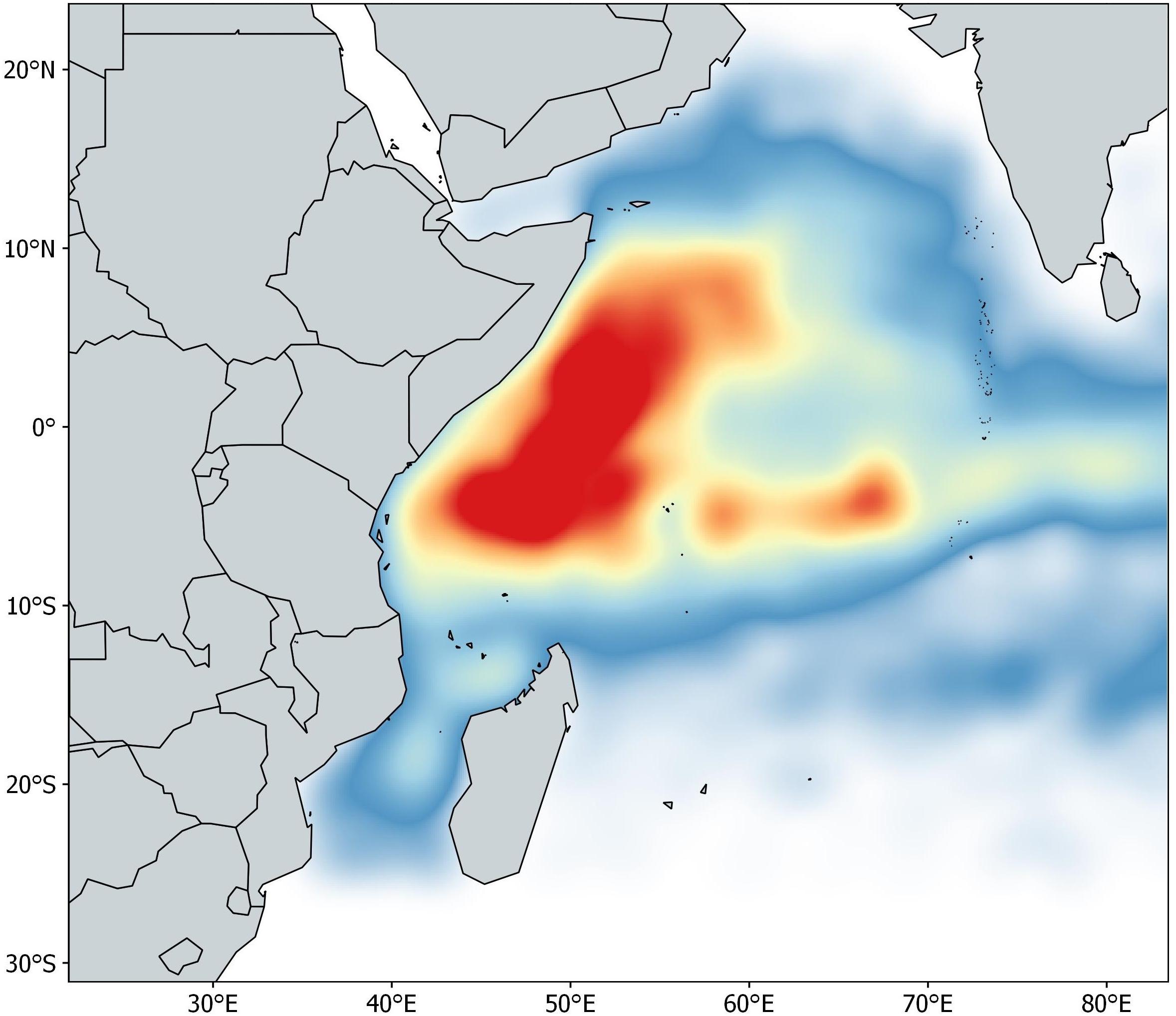
Figure 1. Density map of acoustic samples in the Indian Ocean from January 2012 to May 2015.

For additional validation of the model, the logbooks of the DFADs were collected for the time periods considered in the study. These logbooks have been developed by Spanish national authorities to monitor the fishing activity of the fleet (De Molina et al., 2013).

Autocorrelation (ACF) and Partial Autocorrelation Functions (PACF) were performed to identify annual, seasonal (i.e., monsoonal) and daily non-random temporal patterns in the data using the stats package of the R software (R Development Core Team, 2017). No correlation was found at year level. Non-random distributions of acoustic records were detected for different monsoon seasons and at the daily scale. For this reason, data was aggregated in four different groups following the monsoon pattern of the area: (i) Winter Monsoon (December–March), (ii) Spring Intermonsoon (April–May), (iii) Summer Monsoon (June–September) and (iv) Autumn Intermonsoon (October–November). Day-scale patterns in acoustic records between the 7th and 53rd days did not show autocorrelation and were therefore deemed appropriate for inclusion in the models. Data from the first and last weeks of the time series were removed.

Environmental Data

The environmental variables were obtained from the EU Copernicus Marine Environment Monitoring Service (CMEMS).² Eight abiotic and biotic variables were extracted for each position and date of the acoustic dataset: sea surface temperature (SST), velocity (VEL), and heading (HEADING) of the current, salinity (SAL), eddie kinetic energy (EKE), sea surface height (SSH), chlorophyll concentration (CHL), and oxygen concentration (O2) (Table 1).

TABLE 1

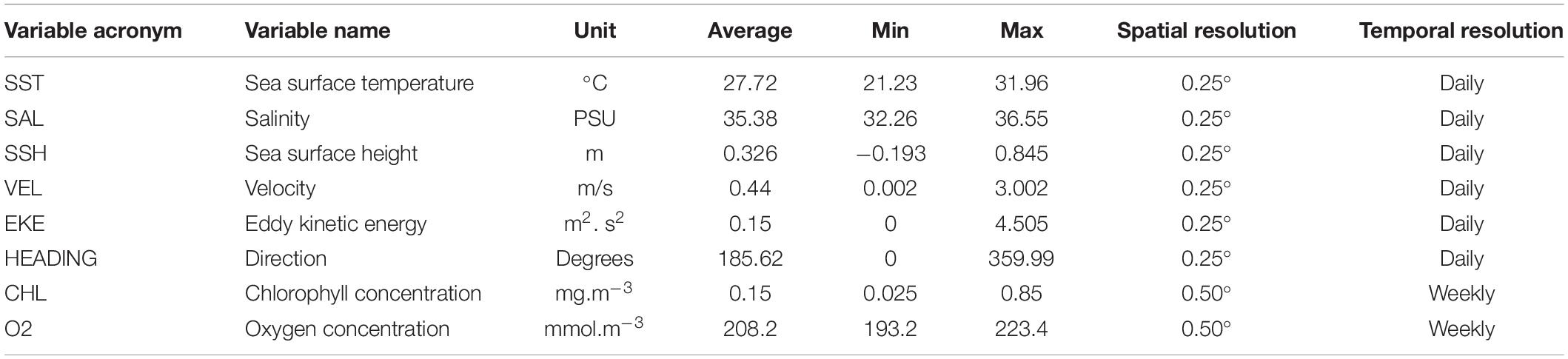
Table 1. Predictor variables used for modeling tuna and non-tuna occurrence with DFAD data in the Indian Ocean.

Before their use in the models, all environmental variables were tested for outliers, missing values and correlation. In addition, collinearity was assessed using the variance inflation factor analysis (VIF) with the function “corvif” in the AED R-package and a cut-off value of 5 (Zuur et al., 2009). Based on these preliminary analyses, velocity was eliminated for the posterior modeling as it was highly correlated with eddie kinetic energy (Pearson correlation, r > 0.9; p-value < 0.001). In order to facilitate interpretation and enable comparison of relative weights between variables (Kinas and Andrade, 2017), these were standardized using the function “decostand” in the vegan R-package (Oksanen et al., 2013). Moreover, days at sea (i.e., time spent in the water since initial deployment) was also included in the models as explanatory variable.

Bayesian Hierarchical Spatial Models (B-HSMs)

B-HSMs (Muñoz et al., 2013) were used to investigate the relationship of tuna and non-tuna species with the selected environmental variables and to obtain the predicted spatio-temporal probability of presence of these groups. In addition to the environmental variables and days at sea, buoy ID was included in the models as a random effect to verify its relevance and account of possible sampling structure autocorrelation. A buoy’s individual behavior due to random factors or non-observed characteristics may have caused some variability in the data. Ignoring such non-independence may result in an invalid statistical inference (Sainani, 2010). Thus, the buoy ID was included in the models to remove any buoy-specific bias (Lopez et al., 2017b).

In the B-HSM framework we used, Y_i represents the species group (i.e., tuna and non-tuna) occurrence (1 being presence; 0 being absence) for each location i, and then the occurrence was modeled as:

$$Y_i\sim \mathit{Bernoulli}\left({\mathrm{\pi }}_i\right)i=1,\mathrm{\dots }.,p$$

$${\mathit{log}}_{\left({\mathrm{\pi }}_i\right)}=X_i\mathrm{\beta }+Z_i+W_i$$

$$\mathrm{\beta }\sim N({\mathrm{\mu }}_{\mathrm{\beta }},q_{\mathrm{\beta }})$$

$$W_i=N(0,Q(k,\mathrm{\tau })$$

$$2\mathit{logk}=N({\mathrm{\mu }}_k,{\mathrm{\rho }}_k)$$

$$2\mathit{log}\mathrm{\tau }=N({\mathrm{\mu }}_{\mathrm{\tau }},{\mathrm{\rho }}_{\mathrm{\tau }})$$

where π_i is the probability of presence of a species for a specific location i, X_iβ is the matrix of the fixed effects of the linear predictor, Z_i is the buoy random effect and Wi represents the spatially structured random effect at location i. In particular W_i, account for the spatial correlation among observations at nearby locations. As required by the Bayesian approach prior distributions were assigned to every parameter of the model. For W_i we assumed a prior Gaussian distribution with a zero mean and a Matérn covariance function, which depends on the hyperparameters k and τ, that represents its range and variance. The range was fixed as the 20% of the diameter of the region and the variance equal to 1 (Lindgren et al., 2011).

Parameters estimation and prediction were obtained using the Integrated Nested Laplace Approximations (INLA) approach (Rue et al., 2009) and R-INLA package.³ INLA is an alternative to Monte Carlo Markov Chain (MCMC) for fitting a large class of Bayesian models (Rue et al., 2009) and has several advantages over other Bayesian approaches. For example, it is faster (i.e., needs less computing time) since the algorithm is naturally parallelized, which makes possible to take advantage of the new generation of multicore processors (Beguin et al., 2012). The model syntax is straightforward, which permits a great compromise of automation with relatively few lines of code.

For fixed effects, no prior information on the parameters of the model was available, so we used vague prior distributions with a mean of 0 and a variance of 1000 as suggested by Held et al. (2010). Posterior distributions were obtained for each parameter of the model. Unlike traditional frequentist approaches, where the mean and the confidence interval are provided, this type of distribution enables explicit probability statements about parameters. Consequently, values included between the 0.025 and 0.975 quantiles of the posterior distribution represent that the unknown parameter is 95% likely to fall within this region (Dell’Apa et al., 2017).

Model Selection

Explanatory variable selection was performed beginning with all possible interaction terms but only the best combination of variables was chosen based on three different measures: (i) the Watanabe-Akaike information criterion (WAIC) (Watanabe, 2010), (ii) Deviance Information Criterion (DIC) (Spiegelhalter et al., 2002), and (iii) Log-Conditional Predictive Ordinates (LCPO) (Roos and Held, 2011). The smaller the values of these measures, the better the compromise between fit, parsimony, and predictive quality of the model. Thus, we choose the best model based on the best balance between lowest DIC, WAIC, and LCPO values, including only relevant predictors (i.e., those with 95% credibility intervals, not including the zero; Fonseca et al., 2017).

Model Validation

B-HSMs were validated using a cross-validation procedure (Fielding and Bell, 1997). The dataset was randomly split into two main subsets: a training dataset including 80% of the total observations, and a testing dataset with the remaining 20%. The training dataset was used to model the relationship between observed data and the explanatory variables and the testing dataset was used to evaluate the predictions’ accuracy. The validation procedure was repeated 10 times for the best model of each group of species (i.e., tuna or non-tuna species) and the results were averaged over different random subsets. In particular, to evaluate the model’s performance, we used the area under the receiver-operating characteristic curve (AUC) (Fielding and Bell, 1997) and the True Skill Statistic (TSS) (Allouche et al., 2006).

AUC measures the model’s ability to discriminate between sites where the species are present and those in which the species are absent. The values for AUC range from 0 to 1, where 0.5 indicates a performance no better than random, values between 0.6 and 0.9 indicate results of presence/absence different from random, and values > 0.9 are excellent to ensure that the results are non-random (Roos et al., 2015). TSS is a threshold-dependent measure that is not affected by the size of the validation set and corrects AUC for the dependence of prevalence on specificity (i.e., ability to correctly predict absences) and sensitivity (i.e., ability to correctly predict presence) (Allouche et al., 2006). Both statistics are used in combination when evaluating the predictive power of an SDM (Pearson et al., 2006; Brodie et al., 2015).

In addition, a second cross-validation approach was performed for tuna models using an additional fishery-dependent dataset. FAD logbooks were used to verify whether or not the B-HSM predictions matched with catches in the same spatio-temporal window. Fishing sets on DFAD were identified as presences, while visits to DFADs without fishing activity and where no fish were observed were classified as absences, providing 3603 data points for cross-validation. This cross-validation procedure provided additional and complementary AUC and TSS measures.

Model Prediction

The probability of presence was predicted in the rest of the area of interest using Bayesian kriging, which treats the parameters as random variables in order to incorporate uncertainty in the prediction process (see Muñoz et al., 2013 for further information). To predict the relationship between species group and habitat features per season, explanatory variables were aggregated with a seasonal monsoon temporal resolution using the “raster” package (Hijmans et al., 2017).

Finally, with the intention of capturing general patterns in spatial trends, we plot the functional response between selected environmental variables and predicted values using ggplot R- package (Wickham, 2016) to apply a smoothing function. This technique uses locally weighted scatterplot smoothing (lowess), which is an outlier-resistant method to estimate a polynomial regression curve including local bootstrap methods with the percentile technique to gather the original lowess fit change.

Results

Tuna

The best fit B-HSM model included SST, SSH, EKE and days at sea as relevant predictors for tuna presence, in addition to spatial and buoy random effects. All models without these two random effects resulted in higher WAIC, DIC, and LCPO than those with them (Table 2).

TABLE 2

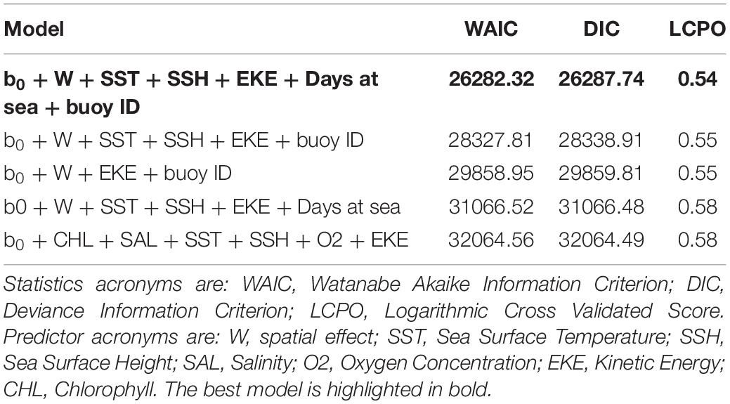
Table 2. Comparison of the most relevant models for the tuna B-HSMs.

Based on the final model, a high probability of tuna presence is expected in warmer surface waters (posterior mean = 0.14; 95% CI = [0.11, 0.17]), with higher values of SSH (posterior mean = 0.16; 95% CI = [0.12, 0.19]) and lower eddy kinetic energy values (posterior mean = −0.18; 95% CI = [−0.22, −0.14]). The probability of tuna presence is also explained by days at sea, indicating higher probabilities when the object stayed more days in the water (posterior mean = 0.03; 95% CI = [0.02, 0.03]) (Table 3). Figure 2 shows that the model found the highest probabilities of tuna presence in warm waters (i.e., between 26 and 30°), moderate SSH values and EKE values around 0.1 m². s².

TABLE 3

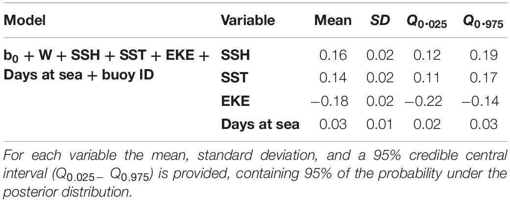
Table 3. Numerical summary of the marginal posterior distribution of the fixed effects for the best tuna B-HSMs selected.

FIGURE 2

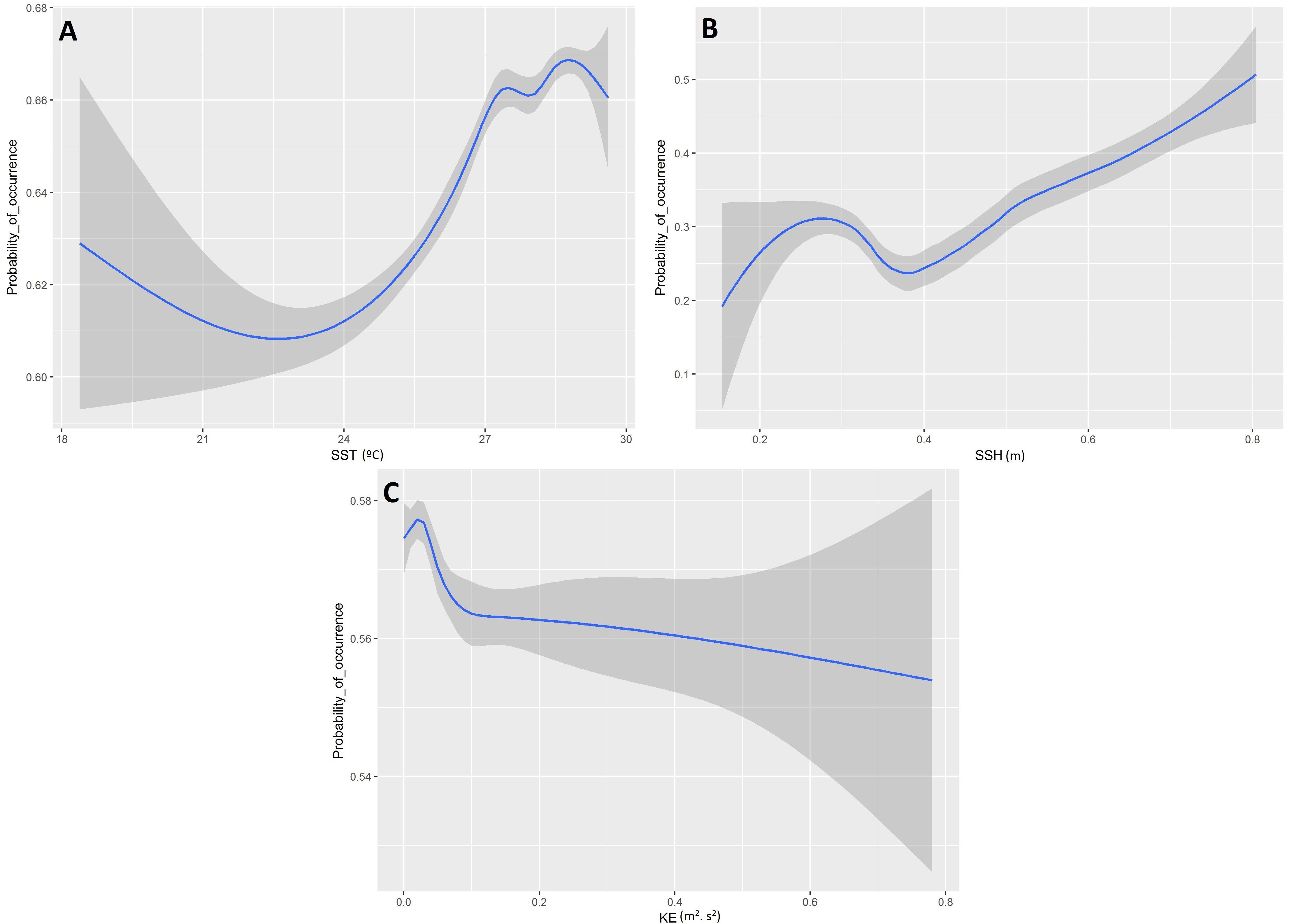
Figure 2. Functional responses of the final tuna B-HSMs (A, Sea Surface Temperature; B, Sea Surface Height; C, Kinetic Energy). The solid line represents the smooth function estimate; the shaded region represents the approximate 95% credibility interval.

Maps of predicted probability of tuna presence show different preferential habitat patterns in monsoon periods (Figure 3). In winter periods two hotspots were observed, one over 10° north and another over 5° south. The main hotspots seem to lay on the equatorial area during the spring inter-monsoon and, then, the probability pattern spreads eastward through the equator during the summer period. During autumn inter-monsoon (October–November), the highest probabilities of tuna presence were found in three well-defined lactations between 0 and 10° south.

FIGURE 3

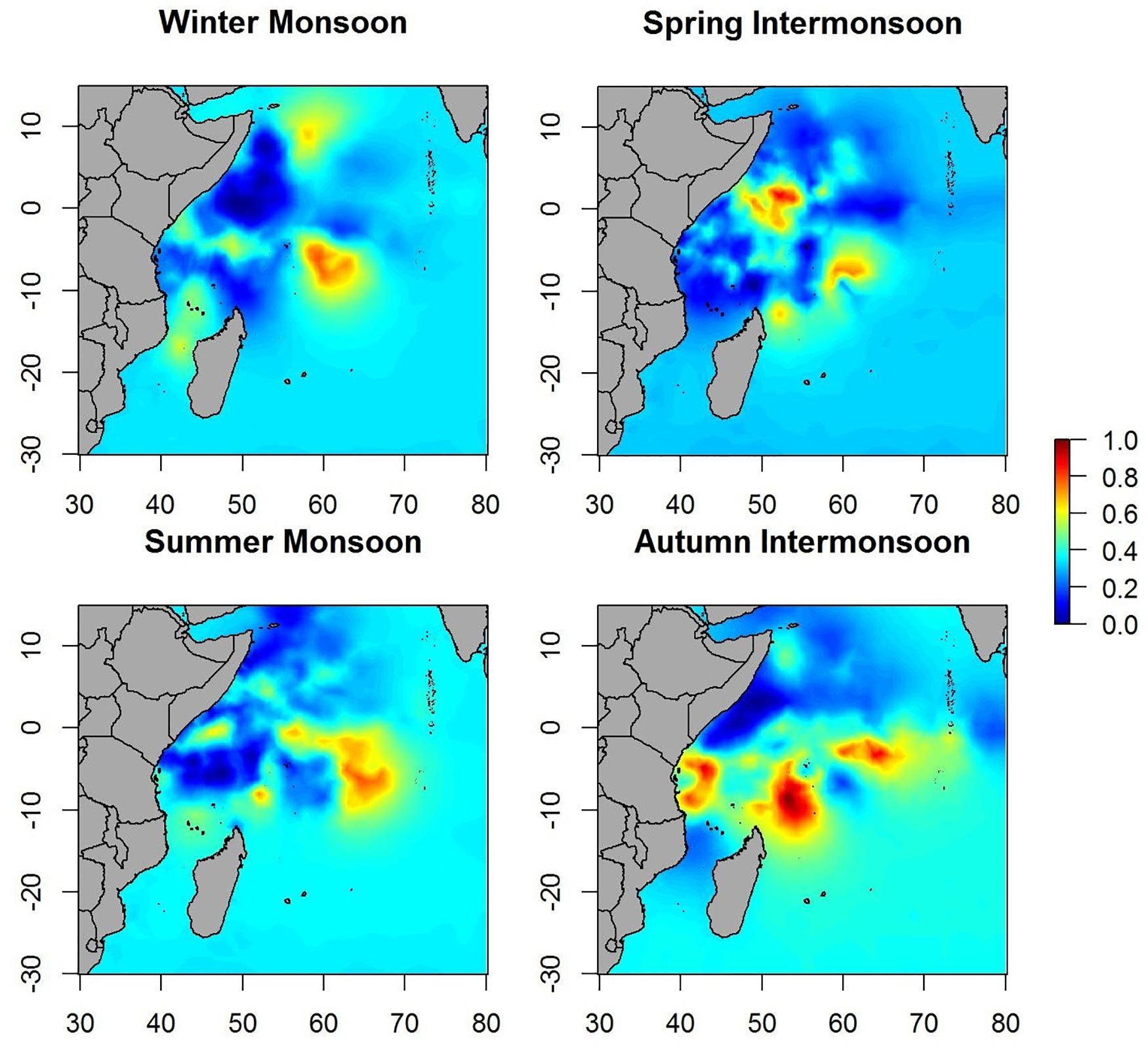
Figure 3. Maps of the posterior mean of tuna occurrence probability in different seasons.

When the spatial effect was included, maps showed similar patterns as when only environmental variables were included. Therefore, most of the variability in the data is explained by the environmental variables included in the B-HSM (Figure 4). Hotspots on spatial effect maps are more marked than on maps of the posterior mean of tuna occurrence probability, which may indicate that there are other ecological processes that are not being considered in this study.

FIGURE 4

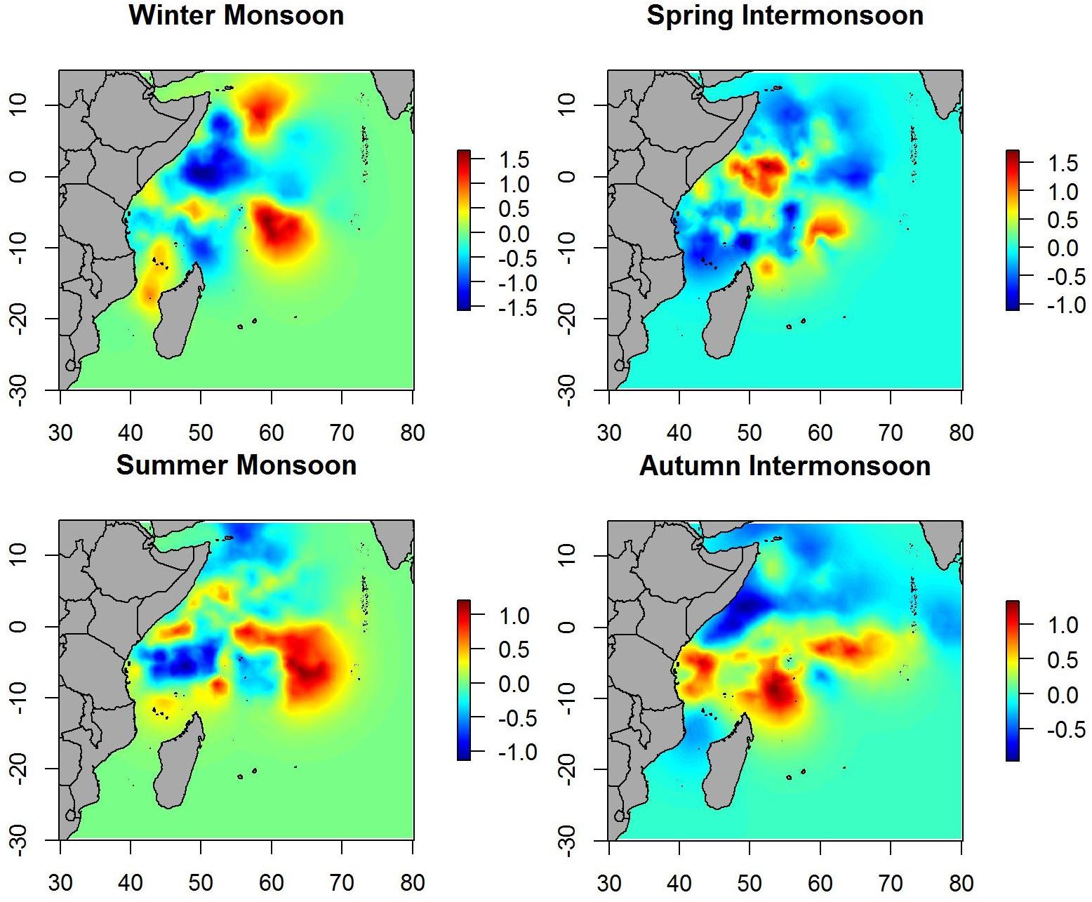
Figure 4. Maps of the posterior mean of the spatial effect for tuna model in different seasons.

Non-tuna Species

The occurrence probability for this group was explained by the SST, the CHL and the days at sea. The final B-HSM for non-tuna species also included spatial and buoy random effects as relevant predictors. As for the tuna B-HSM, all models without these random effects resulted in higher WAIC, DIC and LCPO scores (Table 4).

TABLE 4

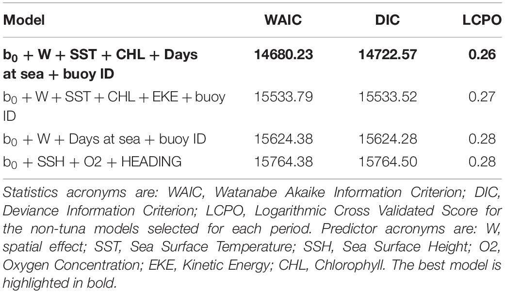
Table 4. Comparison of the most relevant models for the non-tunas B-HSMs.

Higher probabilities of non-tuna species were found in colder (posterior mean = −0.08; 95% CI = [−0.13, −0.03]) and productive waters (posterior mean = 0.11; 95% CI = [0.04, 0.17]). Days at sea was positively related with probability of presence (posterior mean = 0.01; 95% CI = [0.01, 0.02]) although its effect is smaller than in the tuna model, based on the posterior mean values (Table 5). In particular, as shown in Figure 5, the probability of non-tuna presence decreased with temperature continuously from 20°C, while the chlorophyll showed an increasing pattern, with the highest probabilities of non-tuna presence found in waters with chlorophyll concentrations higher than 0.8 mg/m³.

TABLE 5

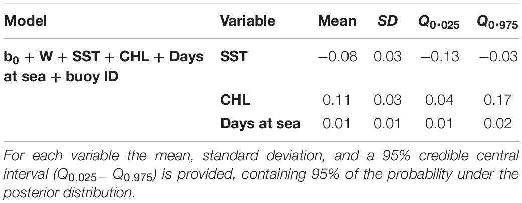
Table 5. Numerical summary of the marginal posterior distribution of the fixed effects for the best non-tuna B-HSM selected.

FIGURE 5

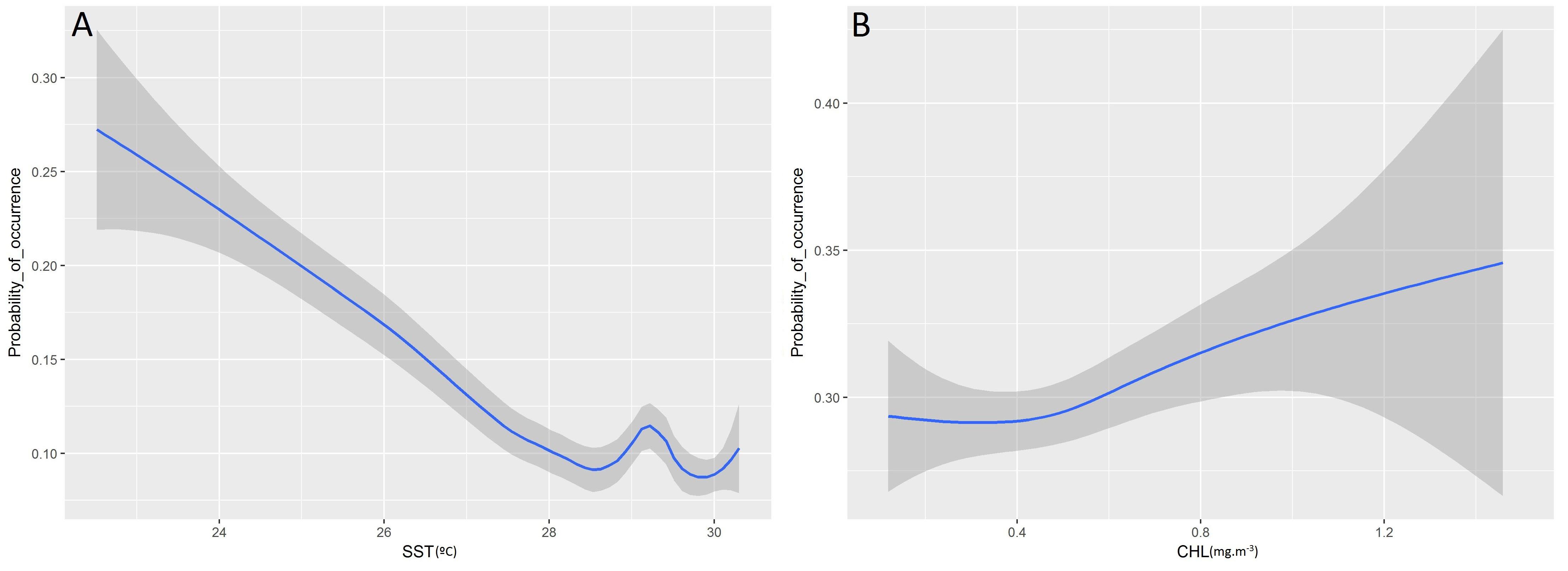
Figure 5. Functional responses of the final non-tuna B-HSMs (A, Sea Surface Temperature; B, Chlorophyll). The solid line represents the smooth function estimate; the shaded region represents the approximate 95% credibility interval.

Maps of the predicted probability of non-tuna species presence identified more marked hotspots during the winter and spring periods, versus scattered hotspots during summer monsoon and autumn inter-monsoon (Figure 6). Throughout the year, intermediate probabilities are found off the coast of Somalia between 0 and 10° north. During the winter period another hotspot in the SE of Seychelles is detected, also for tuna, but less marked.

FIGURE 6

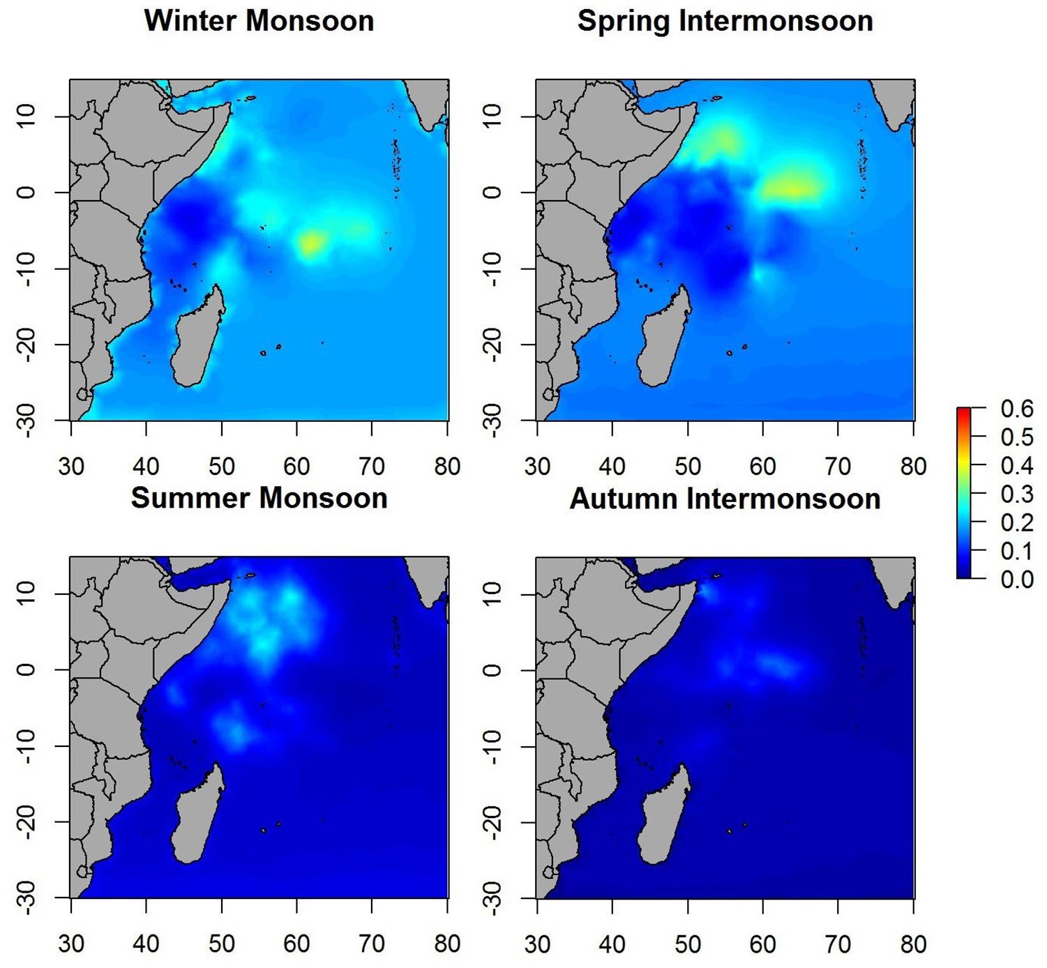
Figure 6. Maps of the posterior mean of non-tuna occurrence probability in different seasons.

Spatial effect maps for non-tuna species showed patterns similar to the posterior mean maps (i.e., although with different scales), which suggests that most of the variability is explained by the variables included in the model (Figure 7).

FIGURE 7

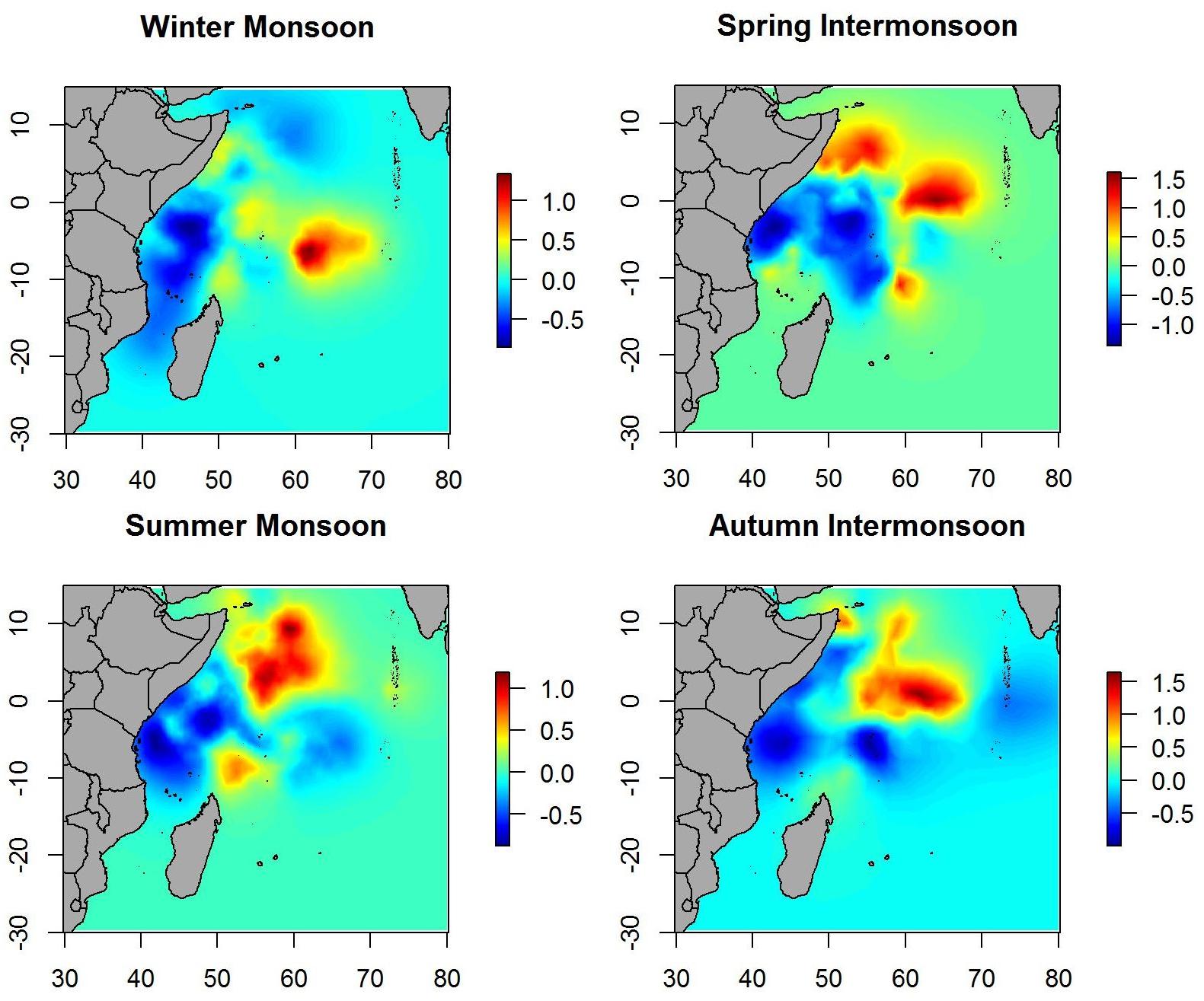
Figure 7. Maps of the posterior mean of the spatial effect of non-tuna in different seasons.

Model Validation

Model prediction performance scores showed AUC values greater than 0.65 (i.e., 0.75 ± 0.07 for tuna models and 0.68 ± 0.06 for non-tuna models), which indicates a good degree of discrimination between locations where tuna and non-tuna groups were present and those where they were absent (Table 2). Likewise, TSS values ranged between 0.20 and 0.39, which represents good model ability to predict true negative and true positive predictions (Brodie et al., 2015). The values of AUC and TSS for the tuna model using the fishery-dependent dataset (i.e., catch and DFADs activities information from fishing and FAD logbooks respectively) achieved lower values than the ones obtained from the echo-sounder estimated presence by B-HSMs (Table 6). However, AUC and TSS values were reasonable, 0.60 ± 0.06 and 0.18 ± 0.08, respectively, indicating good prediction performance for the models.

TABLE 6

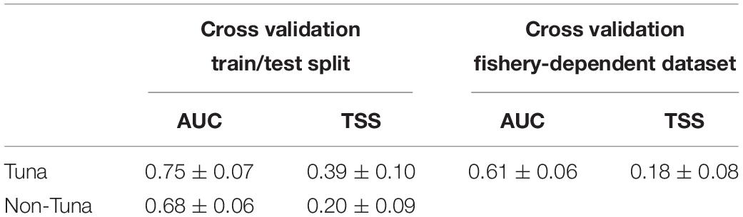
Table 6. Average and standard deviation AUC and TSS values for the final models selected in each case for tuna and non-tuna species using two different datasets (fisheries-independent and fisheries-dependent) for the cross-validation.

Discussion

This study represents the first investigation of the spatial and temporal distribution of tropical tuna and non-tuna species aggregated under DFADs in the Indian Ocean using fishery-independent data collected by fishers’ echo-sounder buoys. The results showed species-specific distribution patterns based on relevant environmental preferences and provide new insights on species habitat when associated with DFADs. Despite tuna and tuna-like species being the most important resources exploited by a variety of fleets operating in the Indian Ocean, detailed studies of their habitat and ecological preferences are limited. Previous knowledge of the distribution dynamics and environmental preferences of tropical tuna in the Indian Ocean have primarily been obtained from fishery-dependent data of purse seiners and longlines fisheries (Chen et al., 2005; Lee et al., 2005; Fonteneau et al., 2008; Song et al., 2008, 2009; Tew-Kai and Marsac, 2009; Lan et al., 2013; Lumban-Gaol et al., 2015), but not fisheries-independent data. Furthermore, only a few studies have considered tuna and other species associated with DFADs. Therefore, the relationship of DFAD-associated species and their local environment is still unclear (Fraile et al., 2010). To our knowledge, only one other study has used acoustic data collected by fishers’ echo-sounder buoys to relate the biomass gathered under the objects to environmental factors, but it was focused on the Atlantic Ocean (Lopez et al., 2017b).

Differing species-specific environmental preferences are suggested by existing literature, likely reflecting differences in the target data (e.g., body size) and the spatio-temporal bounds of the varied methodologies. For example, Mohri and Nishida (2000) and Song et al. (2008), used fishery data that commonly target adult individuals of yellowfin tuna (Thunnus albacares) to suggest a depth range of 100–180 m for this species. In contrast, Cayré and Marsac (1993) and Dagorn et al. (2006) suggested a depth range of 40–110 m for the same species using electronic tagging for juveniles. Temperature has been used as an explanatory variable for tuna habitat in many studies. Mohri and Nishida (2000) and Song et al. (2008) suggested 15–17°C as an optimal temperature range for yellowfin tuna, while Romena (2001) found 17–20°C using qualitative methods. Romena (2001) also suggested an optimal salinity range of 34.2 to 35 PSU for adults of yellowfin tuna in the Indian Ocean. Dissolved oxygen is another important factor commonly used in these studies. Romena (2001) suggested a range of 2.6–5 mg ⋅ L⁻¹ of dissolved oxygen for yellowfin tuna, while Song et al. (2008) of 2–3 mg ⋅ L⁻¹. Song et al. (2009) suggested an optimum of chlorophyll-a of 0.090–0.099 mg L^–1 for yellowfin tuna, different from Lee et al. (1999) which used monthly means of sea surface color in the analysis. Similarly, inter-species environmental preference data is varied. For the habitat preference of bigeye tuna, (Thunnus obesus) in the Indian Ocean, Song et al. (2009) showed an optimal range of 240–280 m of depth, 12–14°C of temperature, and 2–3 mg ⋅ L⁻¹ of dissolved oxygen, whereas for skipjack (Katsuwonus pelamis) sea surface temperature varied between 15 and 30°C (Barkley et al., 1978) and a preferred range from 23 to 28°C (Arrizabalaga et al., 2015). Aggregating these complimentary datasets provides greater overall insight on the tuna environmental preference in the Indian Ocean.

The species-specific temporal distributions found in this study suggest that both tuna and non-tuna species associated with DFADs may have different habitat preferences depending on the monsoon period. These results are consistent with previous studies in which regular seasonal variability in catch has been observed (Kaplan et al., 2014) as well as different spatial patterns in fishing effort in fleet behavior during the monsoon period in the Indian Ocean (Davies et al., 2014a). We note that the temporal scale (e.g., daily, monthly, seasonal or monsoon aggregation) could be case-dependent. Here, we selected the monsoon aggregation on the basis of the ACF and PACF analysis after testing daily and monthly aggregations in B-HSMs and achieving worse predictions and fits (in terms of WAIC, and LCPO). However, others temporal scales (e.g., quarterly) could provide different results, therefore comparative studies are needed to assess the appropriate temporal aggregations (Pennino et al., 2019).

A major difference in this study with respect to fisheries-dependent studies (e.g., Davies et al., 2014a) is that we did not find high probability of presence in the Mozambique Channel throughout the year. However, it is known that the purse seine fisheries have recorded consistent annual catches in this area since 1985 and large quantities of tunas associated to floating objects within this local fishery yearly in March (end of the winter monsoon) and in April–May (inter-monsoon). Model bias likely explains the absence of probability of presence for this area and timeframe. First, this model has a lower prediction power in areas with few or no observations. Second, B-HSMs implicitly assume that correlation is only dependent on the distance between observations, and therefore does not account for the presence of physical barriers– in this case, the island of Madagascar. Efforts to account for spatial disruptions within current model algorithms are in development (Martínez-Minaya et al., 2019). Moreover, there are some differences between our presence probability maps and fishery catch distribution maps. This could be because the probability of occurrence may show different spatio-temporal trends than biomass abundance or catch. For example, for some species, measures of occurrence and measures of abundance respond differently to environmental variables (Heinänen et al., 2008) depending on the life habits, age-size, and trophic niche.

Understanding the habitat characteristics and dynamics of pelagic species aggregated under DFADs contributes to the management and design of conservation measures for these valuable fishery resources, for example, by providing a baseline for the design of area closures, which is especially important in a changing ocean. Currently, the vast majority of spatial management measures for marine species, such as Marine Protected Areas (MPA), set fixed boundaries around mobile species (Hyrenbach et al., 2000; Norse et al., 2005; Crowder and Norse, 2008), which may be rendered inadequate by the dynamism of the ocean. In recent years, the concept of dynamic ocean management has been defined as “management that changes in space and time in response to the shifting nature of the ocean and its users based on the integration of new biological, oceanographic, social and/or economic data in near real-time” (Maxwell et al., 2015). This concept requires more precise data and faster collection, processing, and analysis to enable near real-time responses (Wilson et al., 2018). The approach used in this study could be the first steps toward designing, in the near future, spatio-temporal conservation management measures (e.g., area closures) for both target and non-target species, using near real-time habitat predictions based on acoustic data provided by fishers’ echo-sounders and remote sensing systems.

Environmental Predictors of Species Distribution

This study showed that the spatio-temporal distribution and relevant environmental factors were different for tuna and non-tuna species aggregated at DFADs, suggesting that tuna and non-tuna species may have different habitat preferences.

Tuna

B-HSM results highlighted the importance of SST, SSH, EKE and days at sea for tuna presence. In particular, these results suggest that areas with higher SST and SSH and lower EKE yielded higher probability of tuna presence.

The negative effect with eddy kinetic energy may be due to the energetic cost of being associated with fast-DFADs. This relationship can be observed during summer and in autumn inter-monsoon, when the North Equatorial Current reverses its directions toward the east and combines with the eastward-flowing Equatorial Countercurrent, such that its broad eastward flow dominates the northern Indian Ocean (Benny, 2002). The probability of tuna presence is close to zero during this period above 0°N probably due to the high speed of the buoys that flow with this current eastwards at high speeds (Schott and McCreary, 2001; Tomczak and Godfrey, 2013). This result is consistent with the study of Lopez et al. (2017b), in which tuna predilection to associate with DFADs at speeds between 0.5 and 1 kn or lower was shown. Additionally, in a study by Moreno et al. (2007a) to better understand tuna behavior at DFADs in Indian Ocean, fishers who were interviewed believe that fish leave DFADs when a significant change in the DFAD speed or change in the direction of the trajectory occurs.

Sea surface height was also relevant for the tuna model, presenting a positive relationship with tuna occurrence. This finding is consistent with previous studies that showed a similar relationship in the three oceans (Druon et al., 2017; Lan et al., 2017). Areas of positive SSH values are usually associated with deeper mixed layer depths (MLDs) (Gaube et al., 2013; Dufois et al., 2014, 2017) and mesoscale features (López-Calderón et al., 2006; Benitez-Nelson et al., 2007; Lopez et al., 2017b), suggesting that tuna may prefer deep and well mixed waters in the center or the edge of productivity structures (e.g., eddies). Higher probabilities of tuna presence were also found in areas with high SST. Tuna’s preference for warm surface waters has been observed in previous investigations, where warm waters have been linked to both higher catch rates of large tunas (Zagaglia et al., 2004; Lan et al., 2011, 2017) and acoustic biomass data (Lopez et al., 2017b). Overall, B-HSM results are in accordance with previous studies in the field, which suggest that tropical tunas usually prefer warmer environments that display near null or positive SSH values (Arrizabalaga et al., 2015; Lan et al., 2017; Lopez et al., 2017b).

One uncommon result in this study is a low probability of tuna in the Mozambique Channel area throughout the year. Our methodology only considered DFADs deployed by a single fishing company, and having known trajectories since their deployment. Buoys deployed on natural objects were excluded, because their soak time could not be accurately determined. High abundances of natural floating objects have been observed in the Mozambique Canal (Dagorn et al., 2013), so there have always been fewer deployments of DFADs in this area than in the rest of the Indian Ocean (Davies et al., 2014b). Incorporation of data from this area would provide information complimentary to our study.

A positive relationship was also identified between tuna occurrence and the number of days that the DFAD were at sea, meaning that the longer the DFAD spends in the water, the higher its probability of aggregating tuna. This positive relationship is probably related to the colonization process of the DFADs and is in accordance with other studies (Lopez et al., 2017b; Orue et al., 2019b) showing that, in general, biomass increases with time at DFADs. DFADs may contribute to the formation of large schools of fish and shaping the optimal size of the school (Pitcher and Parrish, 1993) during the first 30–60 days at sea (Orue et al., 2019b). This study only considers DFADs that have stayed at sea 60 days. Additional studies should try to include longer time series in the analysis and test the importance this variable has in the long-term processes associated with DFADs ecology.

The echo-sounder buoys used in this study provide a single value of tuna biomass that includes the three associated species under the DFADs so, for the moment, the specific distribution of each species cannot be analyzed. This has been widely discussed in other studies, where the need for multi-frequency studies on echo-sounder buoys has been highlighted for more effective tuna species discrimination at DFADs (Moreno et al., 2019; Orue et al., 2019b). Once it is possible to effectively discriminate between the three tropical tuna species associated with DFADs, further analyses should identify differences in species behavior and environmental variables.

Non-tuna Species

For non-tuna species, the probabilities of presence were, in general, lower than for the tuna group where the maps of the posterior mean probability show less marked hotspots. This may be related to the buoy detection ability. The buoy used in this study has a blanking zone (i.e., a data exclusion zone to remove transducer’s near-field effect; Simmonds and MacLennan, 2005) between 0 and 3 m, so species located at distances closer from the DFAD are not easily detected by the beam. In this case, we do not believe that the detectability limit will greatly affect outcomes, since some by-catch species are known to be strongly and tightly associated with the DFAD (intranatant/extranatant species, see Freon and Dagorn, 2000) and thus, may be more easily detected. The minimum detection threshold calculated by the buoy (i.e., 1 ton) may be important for non-tuna species, as bycatch species are usually found in DFADs in relatively low biomass (Romanov, 2002, 2008; Amandé et al., 2008; Dagorn et al., 2012; Ruiz et al., 2018). However, as has been explained in previous studies using this buoy brand (Orue et al., 2019b), due to the empirical algorithm used to convert raw acoustic backscatter into biomass, one ton of biomass determined through the skipjack-based algorithm may not necessarily represent the same quantity of non-target species, but certainly less, suggesting that the one ton threshold may not have impacted results significantly. Although we do not believe that these limitations have important implications for the final results, they may affect, to some extent, the smaller estimated probabilities of non-tuna presence.

In this case, the most relevant environmental variables were CHL and again, SST, although in this case the relationship with surface temperature was negative. The negative relationship between SST and non-tuna species presence, and the positive one with CHL, indicates that non-tuna species may show predilection to cold, high productivity waters. In the monsoon predictions, we found a relatively stable area throughout the year with the highest probability of non-tuna presence off the coast of Somalia, which is characterized by the chlorophyll-rich water (Jury et al., 2010). These results are in accordance with published research that investigated the environmental preferences of non-tuna species associated with DFADs in the Atlantic Ocean (Lopez et al., 2017b). The most marked hotspots during the spring period coincide with the Great Whirl, an anticyclonic eddy generated by the Somali current. Although the eddy is usually evident between June and September, the Great Whirl’s anticyclonic circulation reveals on average in April (Beal and Donohue, 2013). Non-tuna probability presence, as well as for tuna, is positively correlated with days at sea. This finding is consistent with a previous study that used fishery-independent data which showed increasing non-tuna biomass the longer the DFAD is at sea (Orue et al., 2019b).

Random Effects for Species Distribution

Results showed that the buoy random effect was relevant to explain part of the variability in the distribution of both tuna and non-tuna species that is not explained by the environment. These results could indicate that other processes driving the associative behavior of tuna and non-tuna species at DFADs have not been incorporated in this study. Some of these may be characteristics associated to the structure of the DFAD. In fact, fishers state that characteristics of the construction can have direct impacts on the effectiveness of the DFAD for fish attraction (Moreno et al., 2016c). For example, fishers build objects with float depth and underwater features dependent on the ocean, and evidence has been provided of a significant relationship between DFAD depth and the colonization of tuna in the Indian Ocean (Orue et al., 2019b).

The spatial effects, which explain the intrinsic spatial variability of the data without the use of explanatory variables, showed similar patterns in probability maps for both tuna as well as non-tuna species. Indeed, maps of the spatial effects highlighted the same hotspots identified in the response variables, although the patterns are more marked than for the models without spatial effects. This is especially true for non-tuna species, which may suggest that part of the variability of DFAD data is not explained by the selected variables. This suggests that other ecological processes not considered in this study may be implicated in the process of species aggregation in DFADs at different scales (e.g., social behavior of tuna at DFADs, FAD densities in the area, dispersal or the patterns of aggregative species). This is consistent with previous studies, where environmental factors were seen to have a more important role in free schools than in DFAD communities in the Indian Ocean (Lezama-Ochoa et al., 2015). Therefore, we could hypothesize that for small tuna that usually aggregate with DFADs, the importance of environmental conditions are not as relevant as for big tunas, which are usually found in free swimming schools. Marsac et al. (2000), raising the ecological trap hypothesis, suggested the possibility that tuna could be trapped in DFADs even when environmental conditions were not biologically optimal, which may affect natural migration routes of tunas and potentially their biology if habited in poor feeding conditions. Future studies should analyze the comparison of preferential/non-preferential areas and biomass aggregation/decrease around DFADs, which could inform the effect of DFADs on tuna and non-tuna species movement and habitat, and shed light on the ecological trap hypothesis.

Dataset Features and Statistical Reliance

Large-scale habitat preference predictions, such as those carried out in this study, allow wider and more comprehensive knowledge of species distribution, although their use can result in a certain level of compromise in the analysis. Mapping of critical habitats requires a high level of accuracy, but the problem is that the amount of data available over large areas is often limited or very aggregated in certain regions. Bayesian interpolation and extrapolation are sufficiently reliable for the identification of species distribution for effective decision making in fishery management. The use of B-HSM for habitat identification is founded on a number of predictive evaluation criteria that prove a reasonable predictive performance for this approach and its benefits in terms of ecological interpretation. Fishery-dependent datasets matched, in general with various exceptions due to lack of data in those regions, the predicted presences of the fishery-independent data and Bayesian distribution models with a reasonable level of accuracy, as shown by the TSS and AUC indexes.

The use of monsoon seasons, which are not consistent with seasonal catch and catch rates of the DFAD fishery, coupled with the limited DFAD buoy information in some areas or seasons means that the model does not predict the probability of tuna occurrence in areas or seasons where fishing hotspots usually occur (i.e., Somalia area each year accounting for large amount of DFAD catches and Mozambique area where a seasonal fishery take place during March, April and May). Therefore, the present results and conclusions should be taken with caution due to the limited DFAD buoy data analyzed. Future work should be devoted to apply same approach using data covering the entire Indian Ocean consistently.

Conclusion

The B-HSM used in this study provides a description of the seasonal distribution of tuna and non-tuna species associated to DFADs in the Indian Ocean using large-scale, non-invasive sampling, and identifies the suitable and preferential areas of these species’ groups. However, these results and conclusions should be taken with caution due to the limited data from DFAD buoys analyzed. The vast majority of management measures for marine species set fixed boundaries around mobile species (Hyrenbach et al., 2000; Norse et al., 2005), which is not very useful for species like tuna as they are highly mobile. DFADs attached to echo sounder buoys continuously record and provide information on the DFADs trajectories as well as the biomass of fish aggregated below them, so they may represent powerful tools for the study of pelagic ecosystems in a dynamic way (Moreno et al., 2016a). The approach used in this study could be very useful to help designing spatio-temporal conservation management measures, using near real-time habitat predictions based on acoustic data provided by fishers’ echo-sounders and remote sensing systems. Nevertheless, much work remains to be done, especially related to the improvement of biomass estimation by echo-sounders buoys. Moreover, none of the echo-sounders used at this time have the ability to discriminate fish species and sizes, since these buoys operate with a single frequency. If echo-sounder buoys had the capability to directly identify this information of tunas found at DFADs, these real-time habitat predictions could provide specific management measures for certain species or sizes. Making this possible will require initiatives of data-exchange between fleets and scientific organizations, which allow, either directly or with certain delay, the transmission of echo-sounder buoy data to scientists.

Data Availability Statement

The datasets for this article are not publicly available because they reflect individual fishing strategies of a private fishing vessel company. Requests to access the datasets should be directed to the company by contacting Julen Marques from Echebastar (julen@echebastar.com).

Author Contributions

BO, MP, HM, GM, LR, and JL designed the research. BO, MP, HM, GM, and JL performed the research. BO and MP analyzed the data. BO, MP, JL, GM, JS, LR, and HM wrote the manuscript.

Funding

This study was partly funded by a Ph.D. grant by the AZTI Foundation to BO.

Conflict of Interest

The authors declare that the research was conducted in the absence of any commercial or financial relationships that could be construed as a potential conflict of interest.

Acknowledgments

We would like to thank Spanish fishing company Echebastar who kindly agreed to provide the acoustic data from their echo-sounder buoys used in the present study. We would also like to thank the reviewers who helped us to improve the first version of the manuscript. Also, we extend our appreciation to Dr. Emma J. Harrison for helping with the written language. This manuscript is contribution No. 974 from AZTI-Tecnalia, Marine Research Division.

Footnotes

1. ^ www.satlink.es
2. ^ http://marine.copernicus.eu/
3. ^ www.r-inla.org

References

Allouche, O., Tsoar, A., and Kadmon, R. (2006). Assessing the accuracy of species distribution models: prevalence, kappa and the true skill statistic (TSS). J. Appl. Ecol. 43, 1223–1232. doi: 10.1111/j.1365-2664.2006.01214.x

CrossRef Full Text | Google Scholar

Amandé, J. M., Ariz, J., Chassot, E., Chavance, P., Delgado De Molina, A., Gaertner, D., et al. (2008). By-Catch and Discards of the European Purse Seine Tuna Fishery in the Indian Ocean Estimation and Characteristics for the 2003-2007 Period. IOTC-2008-WPEB-12. Victoria: Indian Ocean Tuna Commission.

Google Scholar

Anderson, R., Lew, D., and Peterson, A. (2003). Evaluating predictive models of species’ distributions: criteria for selecting optimal models. Ecol. Modell. 162, 211–232. doi: 10.1016/s0304-3800(02)00349-6

CrossRef Full Text | Google Scholar

Angel, M. V. (1993). Biodiversity of the pelagic ocean. Conserv. Biol. 7, 760–772. doi: 10.1046/j.1523-1739.1993.740760.x

CrossRef Full Text | Google Scholar

Arrizabalaga, H., Dufour, F., Kell, L., Merino, G., Ibaibarriaga, L., Chust, G., et al. (2015). Global habitat preferences of commercially valuable tuna. Deep Sea Res. II Top. Stud. Oceanogr. 113, 102–112. doi: 10.1016/j.dsr2.2014.07.001

CrossRef Full Text | Google Scholar

Báez, J. C., Fernández, F., Pascual-Alayón, P. J., Ramos, M. L., Deniz, S., and Abascal, F. (2018). Updating the Statistics of the EU-Spain Purse Seine Fleet in the Indian Ocean (1990-2017). Victoria: Indian Ocean Tuna Commission.

Google Scholar

Banerjee, S., Carlin, B. P., and Gelfand, A. E. (2014). Hierarchical Modeling and Analysis for Spatial Data. Boca Raton, FL: CRC Press.

Google Scholar

Barkley, R. A., Neill, W. H., and Gooding, R. M. (1978). Skipjack tuna, Katsuwonus pelamis, habitat based on temperature and oxygen requirements. Fish. Bull. 76, 653–662.

Google Scholar

Beal, L., and Donohue, K. (2013). The great whirl: observations of its seasonal development and interannual variability. J. Geophys. Res. Oceans 118, 1–13. doi: 10.1029/2012jc008198

CrossRef Full Text | Google Scholar

Beguin, J., Martino, S., Rue, H., and Cumming, S. G. (2012). Hierarchical analysis of spatially autocorrelated ecological data using integrated nested Laplace approximation. Methods Ecol. Evol. 3, 921–929. doi: 10.1111/j.2041-210x.2012.00211.x

CrossRef Full Text | Google Scholar

Benitez-Nelson, C. R., Bidigare, R. R., Dickey, T. D., Landry, M. R., Leonard, C. L., Brown, S. L., et al. (2007). Mesoscale eddies drive increased silica export in the subtropical Pacific Ocean. Science 316, 1017–1021. doi: 10.1126/science.1136221

CrossRef Full Text | Google Scholar

Benny, P. N. (2002). Variability of western Indian Ocean currents. Western Indian Ocean J. Mar. Sci. 1, 81–90.

Google Scholar

Brodie, S., Hobday, A. J., Smith, J. A., Everett, J. D., Taylor, M. D., Gray, C. A., et al. (2015). Modelling the oceanic habitats of two pelagic species using recreational fisheries data. Fish. Oceanogr. 24, 463–477. doi: 10.1111/fog.12122

CrossRef Full Text | Google Scholar

Castro, J., Santiago, J., and Santana-Ortega, A. (2002). A general theory on fish aggregation to floating objects: an alternative to the meeting point hypothesis. Rev. Fish Biol. Fish. 11, 255–277.

Google Scholar

Cayré, P. A., and Marsac, F. (1993). Modeling the yellowfin tuna (Thunnus albacares) vertical distribution using sonic tagging results and local environmental parameters. Aquat. Living Resour. 6, 1–14. doi: 10.1051/alr:1993001

CrossRef Full Text | Google Scholar

Chen, I., Lee, P. F., and Tzeng, W. N. (2005). Distribution of albacore (Thunnus alalunga) in the Indian Ocean and its relation to environmental factors. Fish. Oceanogr. 14, 71–80. doi: 10.1111/j.1365-2419.2004.00322.x

CrossRef Full Text | Google Scholar

Coelho, R., Mejuto, J., Domingo, A., Yokawa, K., Liu, K. M., Cortés, E., et al. (2017). Distribution patterns and population structure of the blue shark (Prionace glauca) in the Atlantic and Indian Oceans. Fish Fish. 19, 90–106.

Google Scholar

Costa, T. L., Pennino, M. G., and Mendes, L. F. (2017). Identifying ecological barriers in marine environment: The case study of Dasyatis marianae. Mar. Environ. Res. 125, 1–9. doi: 10.1016/j.marenvres.2016.12.005

CrossRef Full Text | Google Scholar

Costello, C., and Kaffine, D. T. (2010). Marine protected areas in spatial property-rights fisheries. Austral. J. Agric. Resour. Econ. 54, 321–341. doi: 10.1111/j.1467-8489.2010.00495.x

CrossRef Full Text | Google Scholar

Crowder, L., and Norse, E. (2008). Essential ecological insights for marine ecosystem-based management and marine spatial planning. Mar. Policy 32, 772–778. doi: 10.1016/j.marpol.2008.03.012

CrossRef Full Text | Google Scholar

Dagorn, L., Bez, N., Fauvel, T., and Walker, E. (2013). How much do fish aggregating devices (FADs) modify the floating object environment in the ocean? Fish. Oceanogr. 22, 147–153. doi: 10.1111/fog.12014

CrossRef Full Text | Google Scholar

Dagorn, L., Filmalter, J., Forget, F., Amandè, M. J., Hall, M. A., Williams, P., et al. (2012). Targeting bigger schools can reduce ecosystem impacts of fisheries. Can. J. Fish. Aquat. Sci. 69, 1463–1467. doi: 10.1139/f2012-089

CrossRef Full Text | Google Scholar

Dagorn, L., Holland, K. N., and Itano, D. G. (2006). Behavior of yellowfin (Thunnus albacares) and bigeye (T. obesus) tuna in a network of fish aggregating devices (FADs). Mar. Biol. 151, 595–606. doi: 10.1007/s00227-006-0511-1

CrossRef Full Text | Google Scholar

Dagorn, L., Pincock, D., Girard, C., Holland, K., Taquet, M., Sancho, G., et al. (2007). Satellite-linked acoustic receivers to observe behavior of fish in remote areas. Aquat. Living Resour. 20, 307–312. doi: 10.1051/alr:2008001

CrossRef Full Text | Google Scholar

Davies, T. K., Mees, C. C., and Milner-Gulland, E. (2014a). Modelling the spatial behaviour of a tropical tuna purse seine fleet. PLoS One 9:e114037. doi: 10.1371/journal.pone.0114037

CrossRef Full Text | Google Scholar

Davies, T. K., Mees, C. C., and Milner-Gulland, E. (2014b). The past, present and future use of drifting fish aggregating devices (FADs) in the Indian Ocean. Mar. Policy 45, 163–170. doi: 10.1016/j.marpol.2013.12.014

CrossRef Full Text | Google Scholar

De Molina, A. D., Ariz, J., Santana, J., and Rodriguez, S. (2013). EU/Spain Fish Aggregating Device Management Plan. SCRS/2013/029. Victoria: Indian Ocean Tuna Commission.

Google Scholar

Dell’Apa, A., Pennino, M. G., and Bonzek, C. (2017). Modeling the habitat distribution of spiny dogfish (Squalus acanthias), by sex, in coastal waters of the northeastern United States. Fish. Bull. 115, 89–100. doi: 10.7755/fb.115.1.8

CrossRef Full Text | Google Scholar

Dempster, T., and Taquet, M. (2004). Fish aggregation device (FAD) research: gaps in current knowledge and future directions for ecological studies. Rev. Fish Biol. Fish. 14, 21–42. doi: 10.1007/s11160-004-3151-x

CrossRef Full Text | Google Scholar

Druon, J.-N., Chassot, E., Murua, H., and Lopez, J. (2017). Skipjack tuna availability for purse seine fisheries is driven by suitable feeding habitat dynamics in the Atlantic and Indian Oceans. Front. Mar. Sci. 4:315. doi: 10.3389/fmars.2017.00315

CrossRef Full Text | Google Scholar

Dueri, S., and Maury, O. (2013). Modelling the effect of marine protected areas on the population of skipjack tuna in the Indian Ocean. Aquat. Living Resour. 26, 171–178. doi: 10.1051/alr/2012032

CrossRef Full Text | Google Scholar

Dufois, F., Hardman-Mountford, N. J., Fernandes, M., Wojtasiewicz, B., Shenoy, D., Slawinski, D., et al. (2017). Observational insights into chlorophyll distributions of subtropical South Indian Ocean eddies. Geophys. Res. Lett. 44, 3255–3264. doi: 10.1002/2016gl072371

CrossRef Full Text | Google Scholar

Dufois, F., Hardman-Mountford, N. J., Grenwood, J., Richardson, A. J., Feng, M., Herbette, S., et al. (2014). Impact of eddies on surface chlorophyll in the South Indian Ocean. J. Geophys. Res. Oceans 119, 8061–8077. doi: 10.1002/2014jc010164

CrossRef Full Text | Google Scholar

Fielding, A. H., and Bell, J. F. (1997). A review of methods for the assessment of prediction errors in conservation presence/absence models. Environ. Conserv. 24, 38–49. doi: 10.1017/s0376892997000088

CrossRef Full Text | Google Scholar

Filmalter, J. D., Dagorn, L., Cowley, P. D., and Taquet, M. (2011). First descriptions of the behavior of silky sharks, Carcharhinus falciformis, around drifting fish aggregating devices in the Indian Ocean. Bull. Mar. Sci. 87, 325–337. doi: 10.5343/bms.2010.1057

CrossRef Full Text | Google Scholar

Fonseca, V. P., Pennino, M. G., De Nóbrega, M. F., Oliveira, J. E. L., and De Figueiredo Mendes, L. (2017). Identifying fish diversity hot-spots in data-poor situations. Mar. Environ. Res. 129, 365–373. doi: 10.1016/j.marenvres.2017.06.017

CrossRef Full Text | Google Scholar

Fonteneau, A., Chassot, E., and Bodin, N. (2013). Global spatio-temporal patterns in tropical tuna purse seine fisheries on drifting fish aggregating devices (DFADs): taking a historical perspective to inform current challenges. Aquat. Living Resour. 26, 37–48. doi: 10.1051/alr/2013046

CrossRef Full Text | Google Scholar

Fonteneau, A., Lucas, V., Tewkai, E., Delgado, A., and Demarcq, H. (2008). Mesoscale exploitation of a major tuna concentration in the Indian Ocean. Aquat. Living Resour. 21, 109–121. doi: 10.1051/alr:2008028

CrossRef Full Text | Google Scholar

Forget, F. G., Capello, M., Filmalter, J. D., Govinden, R., Soria, M., Cowley, P. D., et al. (2015). Behaviour and vulnerability of target and non-target species at drifting fish aggregating devices (FADs) in the tropical tuna purse seine fishery determined by acoustic telemetry. Can. J. Fish. Aquat. Sci. 72, 1398–1405. doi: 10.1139/cjfas-2014-0458

CrossRef Full Text | Google Scholar

Fraile, I., Murua, H., Goni, N., and Caballero, A. (2010). Effects of Environmental Factors on Catch Rates of FAD-Associated Yellowfin (Thunnus albacares) and Skipjack (Katsuwonus pelamis) Tunas in the Western Indian Ocean. IOTC-2010-WPTT-46. Victoria: Indian Ocean Tuna Commission.

Google Scholar

Freon, P., and Dagorn, L. (2000). Review of fish associative behaviuour: toward a generalisation of the meeting point hypothesis. Rev. Fish Biol. Fish. 10, 183–207.

Google Scholar

Gaube, P., Chelton, D. B., Strutton, P. G., and Behrenfeld, M. J. (2013). Satellite observations of chlorophyll, phytoplankton biomass, and Ekman pumping in nonlinear mesoscale eddies. J. Geophys. Res. Oceans 118, 6349–6370. doi: 10.1002/2013jc009027

CrossRef Full Text | Google Scholar

Gelfand, A. E., Silander, J. A., Wu, S., Latimer, A., Lewis, P. O., Rebelo, A. G., et al. (2006). Explaining species distribution patterns through hierarchical modeling. Bayesian Anal. 1, 41–92. doi: 10.1214/06-ba102

CrossRef Full Text | Google Scholar

Gershman, D., Nickson, A., and O’toole, M. (2015). Estimating The Use of FADS Around the World. Washington, DC: PEW Environmental group.

Google Scholar

Govinden, R., Dagorn, L., Filmalter, J., and Soria, M. (2010). Behaviour of Tuna Associated with Drifting Fish Aggregating Devices (FADs) in the Mozambique Channel. IOTC-2010-WPTT-25. Victoria: Indian Ocean Tuna Commission.

Google Scholar

Guisan, A., Tingley, R., Baumgartner, J. B., Naujokaitis-Lewis, I., Sutcliffe, P. R., Tulloch, A. I, et al. (2013). Predicting species distributions for conservation decisions. Ecol. Lett. 16, 1424–1435.

Google Scholar

Guisan, A., and Zimmermann, N. E. (2000). Predictive habitat distribution models in ecology. Ecol. Model. 135, 147–186. doi: 10.1016/s0304-3800(00)00354-9

CrossRef Full Text | Google Scholar

Haining, R., Law, J., Maheswaran, R., Pearson, T., and Brindley, P. (2007). Bayesian modelling of environmental risk: example using a small area ecological study of coronary heart disease mortality in relation to modelled outdoor nitrogen oxide levels. Stochastic Environ. Res. Risk Assess. 21, 501–509. doi: 10.1007/s00477-007-0134-1

CrossRef Full Text | Google Scholar

Hastie, T. J., and Tibshirani, R. J. (1990). Generalized additive models. Monographs on Statistics and Applied Probability. London: Chapman and Hall/CRC.

Google Scholar

Hazen, E. L., Palacios, D. M., Forney, K. A., Howell, E. A., Becker, E., Hoover, A. L., et al. (2017). WhaleWatch: a dynamic management tool for predicting blue whale density in the California current. J. Appl. Ecol. 54, 1415–1428. doi: 10.1111/1365-2664.12820

CrossRef Full Text | Google Scholar

Heinänen, S., Rönkä, M., and Von Numers, M. (2008). Modelling the occurrence and abundance of a colonial species, the arctic tern Sterna paradisaea in the archipelago of SW Finland. Ecography 31, 601–611. doi: 10.1111/j.0906-7590.2008.05410.x

CrossRef Full Text | Google Scholar

Held, L., Schrödle, B., and Rue, H. (2010). “Posterior and cross-validatory predictive checks: a comparison of MCMC and INLA,” in Statistical Modelling and Regression Structures, eds T. Kneib, and G. Tutz, (Cham: Springer), 91–110. doi: 10.1007/978-3-7908-2413-1_6

CrossRef Full Text | Google Scholar

Hijmans, R., van Etten, J., Cheng, J., Mattiuzzi, M., Sumner, M., Greenberg, J. (2017). Raster: Geographic Data Analysis and Modeling. R Package Version 2.3-33; 2016. Availale online at: https://rspatial.org/raster

Google Scholar

Hyrenbach, K. D., Forney, K. A., and Dayton, P. K. (2000). Marine protected areas and ocean basin management. Aquat. Conserv. Mar. Freshw. Ecosyst. 10, 437–458.

Google Scholar

ISSF (2019). Status of the world fisheries for tuna. Mar. 2019. ISSF Technical Report 2019-07. Washington, DC: Seafood Sustainability Foundation.

Google Scholar

Jury, M., Mcclanahan, T., and Maina, J. (2010). West Indian ocean variability and east African fish catch. Mar. Environ. Res. 70, 162–170. doi: 10.1016/j.marenvres.2010.04.006

CrossRef Full Text | Google Scholar

Kaplan, D., Chassot, E., Gruss, A., and Fonteneau, A. (2010). Pelagic MPAs: the devil is in the details. Trends Ecol. Evol. 25, 62–63. doi: 10.1016/j.tree.2009.09.003

CrossRef Full Text | Google Scholar

Kaplan, D. M., Chassot, E., Amandé, J. M., Dueri, S., Demarcq, H., Dagorn, L., et al. (2014). Spatial management of Indian Ocean tropical tuna fisheries: potential and perspectives. ICES J. Mar. Sci. J. Conseil 71, 1728–1749. doi: 10.1093/icesjms/fst233

CrossRef Full Text | Google Scholar

Kinas, P. G., and Andrade, H. A. (2017). Introdução à Análise Bayesiana (com R). London: Consultor Editorial Publicações.

Google Scholar

Lan, K.-W., Evans, K., and Lee, M.-A. (2013). Effects of climate variability on the distribution and fishing conditions of yellowfin tuna (Thunnus albacares) in the western Indian Ocean. Clim. Change 119, 63–77. doi: 10.1007/s10584-012-0637-8

CrossRef Full Text | Google Scholar

Lan, K.-W., Lee, M.-A., Lu, H.-J., Shieh, W.-J., Lin, W.-K., and Kao, S.-C. (2011). Ocean variations associated with fishing conditions for yellowfin tuna (Thunnus albacares) in the equatorial Atlantic Ocean. ICES J. Mar. Sci. 68, 1063–1071. doi: 10.1093/icesjms/fsr045

CrossRef Full Text | Google Scholar

Lan, K.-W., Shimada, T., Lee, M.-A., Su, N.-J., and Chang, Y. (2017). Using remote-rensing environmental and fishery data to map potential yellowfin tuna habitats in the tropical Pacific Ocean. Remote Sensing 9:444. doi: 10.3390/rs9050444

CrossRef Full Text | Google Scholar

Lee, P.-F., Chen, I., and Tzeng, W.-N. (2005). Spatial and temporal distribution patterns of bigeye tuna (Thunnus obesus) in the Indian Ocean. Zool. Stud. 44, 260–270.

Google Scholar

Lee, P. F., Chen, I. C., and Tseng, W. N. (1999). “Distribution patterns of three dominant tuna species in the Indian Ocean,” in Proceedings of the 19th International ERSI Users Conference, San Diego, CA.

Google Scholar

Lehodey, P., Senina, I., and Murtugudde, R. (2008). A spatial ecosystem and populations dynamics model (SEAPODYM)–Modeling of tuna and tuna-like populations. Prog. Oceanogr. 78, 304–318. doi: 10.1016/j.pocean.2008.06.004

CrossRef Full Text | Google Scholar

Lezama-Ochoa, N., Murua, H., Chust, G., Ruiz, J., Chavance, P., De Molina, A. D., et al. (2015). Biodiversity in the by-catch communities of the pelagic ecosystem in the Western Indian Ocean. Biodivers. Conserv. 24, 2647–2671. doi: 10.1007/s10531-015-0951-3

CrossRef Full Text | Google Scholar

Lezama-Ochoa, N., Murua, H., Chust, G., Van Loon, E., Ruiz, J., Hall, M., et al. (2016). Present and future potential habitat distribution of Carcharhinus falciformis and Canthidermis maculata by-catch species in the tropical tuna purse-seine fishery under climate change. Front. Mar. Sci. 3:34. doi: 10.3389/fmars.2016.00034

CrossRef Full Text | Google Scholar

Lindgren, F., Rue, H., and Lindström, J. (2011). An explicit link between Gaussian fields and Gaussian Markov random fields: the stochastic partial differential equation approach. J. R. Stat. Soc. Ser. B 73, 423–498. doi: 10.1111/j.1467-9868.2011.00777.x

CrossRef Full Text | Google Scholar

Lopez, J., Moreno, G., Boyra, G., and Dagorn, L. (2016). A model based on data from echosounder buoys to estimate biomass of fish species associated with fish aggregating devices. Fish. Bull. 114, 166–178. doi: 10.7755/fb.114.2.4

CrossRef Full Text | Google Scholar

Lopez, J., Moreno, G., Ibaibarriaga, L., and Dagorn, L. (2017a). Diel behaviour of tuna and non-tuna species at drifting fish aggregating devices (DFADs) in the Western Indian Ocean, determined by fishers’ echo-sounder buoys. Mar. Biol. 164:44.

Google Scholar

Lopez, J., Moreno, G., Lennert-Cody, C., Maunder, M., Sancristobal, I., Caballero, A., et al. (2017b). Environmental preferences of tuna and non-tuna species associated with drifting fish aggregating devices (DFADs) in the Atlantic Ocean, ascertained through fishers’ echo-sounder buoys. Deep Sea Res. II Top. Stud. Oceanogr. 140, 127–138. doi: 10.1016/j.dsr2.2017.02.007

CrossRef Full Text | Google Scholar

Lopez, J., Moreno, G., Sancristobal, I., and Murua, J. (2014). Evolution and current state of the technology of echo-sounder buoys used by Spanish tropical tuna purse seiners in the Atlantic, Indian and Pacific Oceans. Fish. Res. 155, 127–137. doi: 10.1016/j.fishres.2014.02.033

CrossRef Full Text | Google Scholar

López-Calderón, J., Manzo-Monroy, H., Santamaría-Del-Ángel, E., Castro, R., González-Silvera, A., and Millán-Núñez, R. (2006). Mesoscale variability of the Mexican Tropical Pacific using TOPEX and SeaWiFS data. Ciencias Mar. 32, 539–549. doi: 10.7773/cm.v32i3.1125

CrossRef Full Text | Google Scholar

Lumban-Gaol, J., Leben, R. R., Vignudelli, S., Mahapatra, K., Okada, Y., Nababan, B., et al. (2015). Variability of satellite-derived sea surface height anomaly, and its relationship with Bigeye tuna (Thunnus obesus) catch in the Eastern Indian Ocean. Eur. J. Remote Sens. 48, 465–477. doi: 10.5721/eujrs20154826

CrossRef Full Text | Google Scholar

Marsac, F., Fonteneau, A., and Menard, F. (2000). “Drifting FADs used in tuna fisheries: an ecological trap?,” in Proceedings of the Conference on Pêche thonière et dispositifs de concentration de poissons, Martinique, eds J. Y. Le Gall, P. Cayré, and M. Taquet, (Issy-les-Moulineaux: IFREMER), 537–552.

Google Scholar

Martínez-Minaya, J., Cameletti, M., Conesa, D., and Pennino, M. G. (2018). Species distribution modeling: a statistical review with focus in spatio-temporal issues. Stochastic Environ. Res. Risk Assess. 32, 3227–3244. doi: 10.1007/s00477-018-1548-7

CrossRef Full Text | Google Scholar

Martínez-Minaya, J., Conesa, D., Bakka, H., and Pennino, M. G. (2019). Dealing with physical barriers in bottlenose dolphin (Tursiops truncatus) distribution. Ecol. Model. 406, 44–49. doi: 10.1016/j.ecolmodel.2019.05.013

CrossRef Full Text | Google Scholar

Maufroy, A., Kaplan, D. M., Bez, N., De Molina, A. D., Murua, H., Floch, L., et al. (2016). Massive increase in the use of drifting Fish Aggregating Devices (dFADs) by tropical tuna purse seine fisheries in the Atlantic and Indian oceans. ICES J. Mar. Sci. 74, 215–225. doi: 10.1093/icesjms/fsw175

CrossRef Full Text | Google Scholar

Maury, O. (2010). An overview of APECOSM, a spatialized mass balanced “Apex Predators ECOSystem Model” to study physiologically structured tuna population dynamics in their ecosystem. Prog. Oceanogr. 84, 113–117. doi: 10.1016/j.pocean.2009.09.013

CrossRef Full Text | Google Scholar

Maxwell, S. M., Hazen, E. L., Lewison, R. L., Dunn, D. C., Bailey, H., Bograd, S. J., et al. (2015). Dynamic ocean management: defining and conceptualizing real-time management of the ocean. Mar. Policy 58, 42–50. doi: 10.1016/j.marpol.2015.03.014

CrossRef Full Text | Google Scholar

Mohri, M., and Nishida, T. (2000). Consideration on distribution of adult yellowfin tuna (Thunnus albacares) in the Indian Ocean based on Japanese tuna longline fisheries and survey information. J. Natl. Fish. Univ. 49, 1–11.

Google Scholar

Moreno, G., Boyra, G., Sancristobal, I., Itano, D., and Restrepo, V. (2019). Towards acoustic discrimination of tropical tuna associated with fish aggregating devices. PLoS One 14:e0216353. doi: 10.1371/journal.pone.0216353

CrossRef Full Text | Google Scholar

Moreno, G., Dagorn, L., Capello, M., Lopez, J., Filmalter, J., Forget, F., et al. (2016a). Fish aggregating devices (FADs) as scientific platforms. Fish. Res. 178, 122–129. doi: 10.1016/j.fishres.2015.09.021

CrossRef Full Text | Google Scholar

Moreno, G., Dagorn, L., Sancho, G., and Itano, D. (2007a). Fish behaviour from fishers’ knowledge: the case study of tropical tuna around drifting fish aggregating devices (DFADs). Can. J. Fish. Aquat. Sci. 64, 1517–1528. doi: 10.1139/f07-113

CrossRef Full Text | Google Scholar

Moreno, G., Josse, E., Brehmer, P., and Nøttestad, L. (2007b). Echotrace classification and spatial distribution of pelagic fish aggregations around drifting fish aggregating devices (DFAD). Aquat. Living Resour. 20, 343–356. doi: 10.1051/alr:2008015

CrossRef Full Text | Google Scholar

Moreno, G., Murua, J., and Restrepo, V. (2016b). The Use of Echo-Sounder Buoys in Purse Seine Fleets Fishing with DFADs in the Eastern Pacific Ocean. IATTC, SAC-07 INF- C (c). La Jolla, CA: Inter-American Tropical Tuna Commission.

Google Scholar

Moreno, G., Restrepo, V., Dagorn, L., Hall, M., Murua, J., Sancristobal, I., et al. (2016c). Workshop on the Use of Biodegradable Fish Aggregating Devices (FADs). Technical Report 2016-18A. Virginia: International Seafood Sustainability Foundation.

Google Scholar

Muñoz, F., Pennino, M. G., Conesa, D., López-Quílez, A., and Bellido, J. M. (2013). Estimation and prediction of the spatial occurrence of fish species using Bayesian latent Gaussian models. Stochastic Environ. Res. Risk Asses. 27, 1171–1180. doi: 10.1007/s00477-012-0652-3

CrossRef Full Text | Google Scholar

Norse, E. A., Crowder, L. B., Gjerde, K., Hyrenbach, D., Roberts, C., Safina, C., et al. (2005). Place-based ecosystem management in the open ocean. Mar. Conserv. Biol. 8, 302–327.

Google Scholar

Oksanen, J., Blanchet, F. G., Kindt, R., Legendre, P., Minchin, P. R., O’hara, R., et al. (2013). Package ‘vegan’. Community ecology package, version 2.

Google Scholar

Orue, B., Lopez, J., Moreno, G., Santiago, J., Boyra, G., Uranga, J., et al. (2019a). From fisheries to scientific data: a protocol to process information from fishers’ echo-sounder buoys. Fish. Res. 215, 38–43. doi: 10.1016/j.fishres.2019.03.004

CrossRef Full Text | Google Scholar

Orue, B., Lopez, J., Moreno, G., Santiago, J., Soto, M., and Murua, H. (2019b). Aggregation process of drifting fish aggregating devices (DFADs) in the Western Indian Ocean: who arrives first, tuna or non-tuna species? PLoS One 14:e0210435. doi: 10.1371/journal.pone.0210435

CrossRef Full Text | Google Scholar

Paradinas, I. (2017). Species Distribution Modelling in Fisheries Science. Doctoral dissertation, Universitat de València, València.

Google Scholar

Paradinas, I., Conesa, D., Pennino, M. G., Muñoz, F., Fernández, A. M., López-Quílez, A., et al. (2015). Bayesian spatio-temporal approach to identifying fish nurseries by validating persistence areas. Mar. Ecol. Prog. Ser. 528, 245–255. doi: 10.3354/meps11281

CrossRef Full Text | Google Scholar

Pauly, D., Christensen, V., Guénette, S., and Pitcher, T. J. (2002). Towards sustainability in world fisheries. Nature 418:689. doi: 10.1038/nature01017

CrossRef Full Text | Google Scholar

Pearson, R. G., Thuiller, W., Araújo, M. B., Martinez-Meyer, E., Brotons, L., Mcclean, C., et al. (2006). Model-based uncertainty in species range prediction. J. Biogeogr. 33, 1704–1711. doi: 10.1111/j.1365-2699.2006.01460.x

CrossRef Full Text | Google Scholar

Pennino, M. G., Muñoz, F., Conesa, D., López-Quílez, A., and Bellido, J. M. (2014). Bayesian spatio-temporal discard model in a demersal trawl fishery. J. Sea Res. 90, 44–53. doi: 10.1016/j.seares.2014.03.001

CrossRef Full Text | Google Scholar

Pennino, M. G., Vilela, R., and Bellido, J. M. (2019). Effects of environmental data temporal resolution on the performance of species distribution models. J. Mar. Syst. 189, 78–86. doi: 10.1016/j.jmarsys.2018.10.001

CrossRef Full Text | Google Scholar

Phillips, J. C., Leroy, B., Peatman, T., Escalle, L., and Smith, N. (2019). Electronic Tagging Mitigtion of Bigeye and Yellowfin Tuna Juveniles by Purseine Fisheries. WCPFC-SC15-2019/EB-WP-08. Kolonia: WCPFC.

Google Scholar

Phillips, S. J., Anderson, R. P., and Schapire, R. E. (2006). Maximum entropy modeling of species geographic distributions. Ecol. Model. 190, 231–259. doi: 10.1016/j.ecolmodel.2005.03.026

CrossRef Full Text | Google Scholar

Pitcher, T., and Parrish, J. (1993). “Functions of shoaling behaviour in teleosts,” in Behaviour of Teleost Fishes, ed. T. J. Pitcher, (London: Chapman and Hall), 363–439. doi: 10.1007/978-94-011-1578-0_12

CrossRef Full Text | Google Scholar

Potier, M., Bach, P., Ménard, F., and Marsac, F. (2014). Influence of mesoscale features on micronekton and large pelagic fish communities in the Mozambique Channel. Deep Sea Res. II Top. Stud. Oceanogr. 100, 184–199. doi: 10.1016/j.dsr2.2013.10.026

CrossRef Full Text | Google Scholar

R Development Core Team (2017). R: A Language and Environment for Statistical Computing. Vienna: R.Foundation for Statistical Computing.

Google Scholar

Rajapaksha, J. K., Samarakoon, L., and Gunathilaka, A. A. J. K. (2013). Environmental preferences of yellowfin Tuna in the North East Indian Ocean: an application of satellite data to longline catches. Int. J. Fish. Aquat. Sci. 2, 72–80.

Google Scholar

Robert, M., Dagorn, L., Lopez, J., Moreno, G., and Deneubourg, J.-L. (2013). Does social behavior influence the dynamics of aggregations formed by tropical tunas around floating objects? An experimental approach. J. Exp. Mar. Biol. Ecol. 440, 238–243. doi: 10.1016/j.jembe.2013.01.005

CrossRef Full Text | Google Scholar

Romanov, E. V. (2002). Bycatch in the tuna purse-seine fisheries of the western Indian Ocean. Fish. Bull. 100, 90–105.

Google Scholar

Romanov, E. V. (2008). Bycatch and discards in the Soviet purse seine tuna fisheries on FAD-associated schools in the north equatorial area of the Western Indian Ocean. Western Indian Ocean J. Mar. 7, 163–174.

Google Scholar

Romena, N. A. (2001). Factors affecting distribution of adult yellowfin tuna (Thunnus albacares) and its reproductive ecology in the Indian Ocean based on Japanese tuna longline fisheries and survey information. IOTC Proc. 4, 336–389.

Google Scholar

Roos, M., and Held, L. (2011). Sensitivity analysis in Bayesian generalized linear mixed models for binary data. Bayesian Anal. 6, 259–278. doi: 10.1214/11-ba609

CrossRef Full Text | Google Scholar

Roos, N. C., Carvalho, A. R., Lopes, P. F., and Pennino, M. G. (2015). Modeling sensitive parrotfish (Labridae: Scarini) habitats along the Brazilian coast. Mar. Environ. Res. 110, 92–100. doi: 10.1016/j.marenvres.2015.08.005

CrossRef Full Text | Google Scholar

Rue, H., Martino, S., and Chopin, N. (2009). Approximate Bayesian inference for latent Gaussian models by using integrated nested Laplace approximations. J. R. Stat. Soc. Ser. B 71, 319–392. doi: 10.1111/j.1467-9868.2008.00700.x

CrossRef Full Text | Google Scholar

Ruiz, J., Abascal, F. J., Bach, P., Baez, J. C., Cauquil, P., Grande, M., et al. (2018). Bycatch of the European, and Associated Flag, Purse-Seine Tuna Fishery in the Indian Ocean for the Period 2008-2017. IOTC-2018-WPEB14-15. Victoria: Indian Ocean Tuna Commission.

Google Scholar

Sainani, K. (2010). The importance of accounting for correlated observations. P. M. R. 2, 858–861. doi: 10.1016/j.pmrj.2010.07.482

CrossRef Full Text | Google Scholar

Santiago, J., Lopez, J., Moreno, G., Murua, H., Quincoces, I., and Soto, M. (2015). Towards a Tropical Tuna Buoy-derived Abundance Index (TT-BAI). WCPFC-SC12-2016/SA-IP-14. Kolonia: WCPFC.

Google Scholar

Santiago, J., Murua, H., López, J., and Quincoces, I. (2017). Buoy Derived Abundance Indices of Tropical Tunas in the Indian Ocean. IOTC-2017-WGFAD01-13. Victoria: Indian Ocean Tuna Commission.

Google Scholar

Santiago, J., Uranga, J., Quincoces, I., Orue, B., Grande, M., Murua, H., et al. (2019). A Novel Index of Abundance of Juvenile Yellowfin Tuna in the Atlantic Ocean Derived from Echosounder Buoys. SCRS/2019/075. Victoria: Indian Ocean Tuna Commission.

Google Scholar

Schott, F. A., and McCreary, J. P. (2001). The monsoon circulation of the Indian Ocean. Prog. Oceanogr. 51, 1–123. doi: 10.1016/s0079-6611(01)00083-0

CrossRef Full Text | Google Scholar

Schott, F. A., Xie, S. P., and Mccreary, J. P. (2009). Indian Ocean circulation and climate variability. Rev. Geophys. 47:RG1002.

Google Scholar

Scott, G. P., and Lopez, J. (2014). The Use of FADs in Tuna Fisheries. Fisheries IP/B/PECH/IC/2013-123, 70. Brussels: European Parliament.

Google Scholar

Sequeira, A., Mellin, C., Rowat, D., Meekan, M. G., and Bradshaw, C. J. (2012). Ocean-scale prediction of whale shark distribution. Divers. Distrib. 18, 504–518. doi: 10.1111/j.1472-4642.2011.00853.x

CrossRef Full Text | Google Scholar

Simmonds, J., and MacLennan, D. (2005). Fishery Acoustic Theory and Practice. Oxford: Blackwell Scientific Publications.

Google Scholar

Song, L., Zhou, J., Zhou, Y., Nishida, T., Jiang, W., and Wang, J. (2009). Environmental preferences of bigeye tuna, Thunnus obesus, in the Indian Ocean: an application to a longline fishery. Environ. Biol. Fishes 85, 153–171. doi: 10.1007/s10641-009-9474-7

CrossRef Full Text | Google Scholar

Song, L. M., Zhang, Y., Xu, L. X., Jiang, W. X., and Wang, J. Q. (2008). Environmental preferences of longlining for yellowfin tuna (Thunnus albacares) in the tropical high seas of the Indian Ocean. Fish. Oceanogr. 17, 239–253. doi: 10.1111/j.1365-2419.2008.00476.x

CrossRef Full Text | Google Scholar

Spiegelhalter, D. J., Best, N. G., Carlin, B. P., and Van Der Linde, A. (2002). Bayesian measures of model complexity and fit. J. R. Stat. Soc. B 64, 583–639. doi: 10.1111/1467-9868.00353

CrossRef Full Text | Google Scholar

Taquet, M., Dagorn, L., Gaertner, J.-C., Girard, C., Aumerruddy, R., Sancho, G., et al. (2007). Behavior of dolphinfish (Coryphaena hippurus) around drifting FADs as observed from automated acoustic receivers. Aquat. Living Resour. 20, 323–330. doi: 10.1051/alr:2008008

CrossRef Full Text | Google Scholar

Tew-Kai, E., and Marsac, F. (2009). Patterns of variability of sea surface chlorophyll in the Mozambique Channel: a quantitative approach. J. Mar. Syst. 77, 77–88. doi: 10.1016/j.jmarsys.2008.11.007

CrossRef Full Text | Google Scholar

Tomczak, M., and Godfrey, J. S. (2013). Regional Oceanography: An Introduction. Amsterdam: Elsevier.

Google Scholar

Varela, S., Lobo, J. M., and Hortal, J. (2011). Using species distribution models in paleobiogeography: a matter of data, predictors and concepts. Palaeogeogr. Palaeoclimatol. Palaeoecol. 310, 451–463. doi: 10.1016/j.palaeo.2011.07.021

CrossRef Full Text | Google Scholar

Watanabe, S. (2010). Asymptotic equivalence of Bayes cross validation and widely applicable information criterion in singular learning theory. J. Mach. Learn. Res. 11, 3571–3594.

Google Scholar

Wickham, H. (2016). ggplot2: Elegant Graphics for Data Analysis. Cham: Springer.

Google Scholar

Wiggert, J., Murtugudde, R., and Christian, J. (2006). Annual ecosystem variability in the tropical Indian Ocean: Results of a coupled bio-physical ocean general circulation model. Deep Sea Res. II Top. Stud. Oceanogr. 53, 644–676. doi: 10.1016/j.dsr2.2006.01.027

CrossRef Full Text | Google Scholar

Wilson, J. R., Lomonico, S., Bradley, D., Sievanen, L., Dempsey, T., Bell, M., et al. (2018). Adaptive comanagement to achieve climate-ready fisheries. Conserv. Lett. 11:e12452. doi: 10.1111/conl.12452

CrossRef Full Text | Google Scholar

Wyrtki, K. (1973). “Physical oceanography of the Indian Ocean,” in The Biology of the Indian Ocean, eds B. Zeitzschel, and S. A. Gerlach, (Cham: Springer), 18–36. doi: 10.1007/978-3-642-65468-8_3

CrossRef Full Text | Google Scholar

Young, M., and Carr, M. H. (2015). Application of species distribution models to explain and predict the distribution, abundance and assemblage structure of nearshore temperate reef fishes. Divers. Distrib. 21, 1428–1440. doi: 10.1111/ddi.12378

CrossRef Full Text | Google Scholar

Zagaglia, C. R., Lorenzzetti, J. A., and Stech, J. L. (2004). Remote sensing data and longline catches of yellowfin tuna (Thunnus albacares) in the equatorial Atlantic. Remote Sens. Environ. 93, 267–281. doi: 10.1016/j.rse.2004.07.015

CrossRef Full Text | Google Scholar

Zimmermann, N. E., Edwards, T. C., Graham, C. H., Pearman, P. B., and Svenning, J. C. (2010). New trends in species distribution modelling. Ecography 33, 985–989. doi: 10.1111/j.1600-0587.2010.06953.x

CrossRef Full Text | Google Scholar

Zuur, A., Ieno, E., Walker, N., Saveliev, A., and Smith, G. (2009). Mixed Effects Models and Extensions in Ecology with R. New York, NY: Spring Science and Business Media.

Google Scholar