Shifts in Phytoplankton Community Structure Across an Anticyclonic Eddy Revealed From High Spectral Resolution Lidar Scattering Measurements

Introduction

An understanding of phytoplankton community composition and its changes through time is critical for determining the ecological and biogeochemical role of water masses (Richardson and Jackson, 2007; Uitz et al., 2010). Significant variability in phytoplankton community composition, from decadal to seasonal, and basin to meso- and submesoscale, makes this challenging (Vaillancourt et al., 2003; Dandonneau et al., 2004; Anderson et al., 2008). Mesoscale eddies in the western North Atlantic are highly energetic and play a large role in modulating near-surface chlorophyll-a concentrations (Gaube et al., 2014; Gaube and McGillicuddy, 2017). Mesoscale eddies can affect near-surface particle populations by modifying the local mixing field (Dufois et al., 2014; Gaube et al., 2019), trapping and transporting water masses and their associated particle populations over long distances (Lehahn et al., 2011; Gaube et al., 2014), stirring ambient gradients (Chelton et al., 2011), and modulating vertical fluxes of nutrients and particles (McGillicuddy et al., 2007; Falkowski et al., 2011; Gaube et al., 2015).

Satellites have played an important role in characterizing spatiotemporal variability in marine ecosystems and significant progress has been made toward describing phytoplankton community structure from ocean color satellite radiometry (Hood et al., 2006; Mouw et al., 2017). Multiple algorithms for retrieving phytoplankton functional types (PFTs; i.e., phytoplankton groups that share a similar biogeochemical role) are now available and applied in both coastal and open ocean environments (Kostadinov et al., 2010; Werdell et al., 2014; Uitz et al., 2015; Mouw et al., 2017). These algorithms use the magnitude and/or spectral shape of satellite remote-sensing reflectance to derive properties (e.g., chlorophyll, inherent optical properties) associated with different PFTs. In contrast, the ocean-optimized high spectral resolution lidar (HSRL) directly measures the particulate backscattering coefficient (b_bp) and depolarization ratio (δ), measurements which have previously been used to characterize particles in the ocean but with limited validation with in situ measurements (Fry and Voss, 1985; Loisel et al., 2008; Fournier and Neukermans, 2017). The HSRL technique thus has the potential to provide important information for characterizing phytoplankton community composition. Furthermore, the HSRL returns profiles of ocean properties to approximately 2.5–3 optical depths (Schulien et al., 2017) which can yield new insights on the vertical structure of phytoplankton communities.

The Lorenz-Mie theory and T-matrix models, combined with the vector radiative transfer equation, provide a single scattering framework from which we can evaluate how PSD, shape, and refractive index impact the scattering and polarization properties of the incident light. Numerous studies have used these models, in combination with polarization measurements, to distinguish water masses dominated by inorganic particles (Loisel et al., 2008; Lotsberg and Stamnes, 2010). Chami and McKee (2007) used concurrent in situ measurements of scattered light and particle type to derive an empirical relationship based on the degree of polarization that predicts the concentration of inorganic particles to within ±13%.

Mie theory, which assumes that particles are homogeneous spheres, predicts a positive relationship between depolarization and both mean size and refractive index of particles (Loisel et al., 2008). However, no simple relationship exists between the degree of particle asphericity and depolarization (Mishchenko and Travis, 1998). Volten et al. (1998) measured the scattering functions of 15 different phytoplankton species in the laboratory and found no clear relationship between the degree of linear polarization (from 20° to 60°) and particle shape. Instead, the presence of internal cell structures, specifically gas vacuoles, appeared to have a greater effect on the polarization measurements. These results highlight some of the challenges in relating depolarization measurements to changes in phytoplankton taxonomy. In this study, we recognize that these challenges exist, but take the first steps toward relating in situ high spatial resolution phytoplankton community composition measurements with nearly coincident lidar depolarization and backscatter data and investigate the potential significance of our results.

This study presents coincident airborne HSRL and extensive ship measurements across a distinct eddy feature in the subarctic Atlantic Ocean. This unique combination of measurement types is used to provide a case study in the context of Lorenz–Mie theory single scattering framework. The primary goal of the present study is to understand the sources of variability, including phytoplankton community composition changes, in HSRL-retrieved values of δ and b_bp.

Materials and Methods

Field data were collected as part of the North Atlantic Aerosols and Marine Ecosystem Study (NAAMES) field campaign, which consisted of four coordinated ship-aircraft field campaigns conducted between November 2015 and April 2018 (Behrenfeld et al., 2019b). Data presented here were collected across an anticyclonic eddy encountered during the first NAAMES field campaign, with the ship track and study region shown in Figure 1. Continuous underway measurements of conductivity, temperature, and optical properties were collected (SBE9+ thermosalinograph, WETStar fluorometer, WetLabs ECO-BB3, ac-s spectral absorption and attenuation sensor, Sea-Bird Scientific, Bellevue, WA). Discrete water samples were also analyzed for phytoplankton community composition using an imaging flow cytobot (IFCB; McLean Research Labs, Inc., East Falmouth, MA), with an average spatial resolution of 7 km along the ship track. These measurements provide information on the PSD, shape, and taxonomic composition of phytoplankton between ∼8 and 150 μm. Additional flow cytometer measurements (three samples collected across the eddy) were made using a BD Influx Cell Sorter (ICS; BD Biosciences, San Jose, CA) capable of analyzing particles in the ∼0.2–50 μm size range. These measurements provide information on phytoplankton community structure for smaller size classes (pico- and nano-phytoplankton), with the upper size limit largely determined by the volume of water analyzed, ranging from 1 to 2 mL of whole seawater for this study. Changes in in situ bio-optical and phytoplankton properties were related to measurements of δ and b_bp from an ocean-optimized airborne HSRL.

FIGURE 1

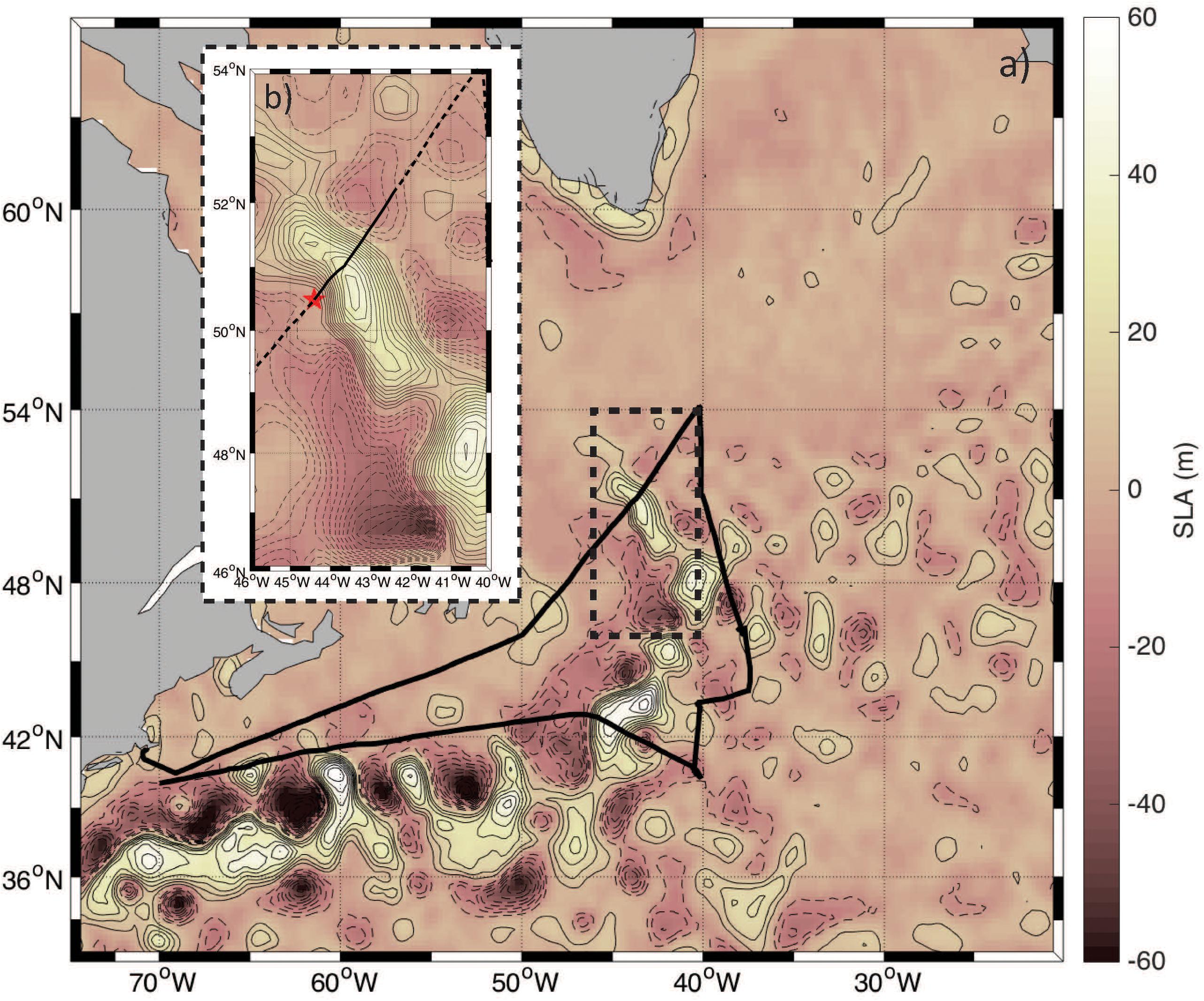
Figure 1. (a) Psudo-color map of sea level anomaly (SLA) overlaid with contours at an interval of 7 cm in the NAAMES study region. Positive SLA (anticyclones) are shown in the solid contours and negative anomalies (cyclones) are displayed by dashed contours. The ship track is indicated by the solid black line and the region analyzed here is bounded in the black hashed box. (b) Zoomed in version of the map shown in panel (a) with a contour interval of 3 cm. The red star indicates the point from which the “Distance along track” is calculated and marks the first measurement collected on November 12, 2015. The solid black line highlights the data collected on November 12, 2015 with the hashed lines indicating data collected before and after this day.

In-Line Measurements

Hyperspectral particulate absorption (a_p) and beam attenuation (c_p) data were collected using an ac-s spectrophotometer installed in a flow-through setup allowing continuous measurements from the ship’s underway intake system located at ∼5 m depth. We diverted the seawater intake line away from the ship’s pump and installed our own diaphragm pump to minimize disturbances to particle assemblages. Particulate spectra were obtained by differencing water passed through a 0.2 μm filter from total water, where the water was directed automatically through the filter for 10 min h^–1 (Slade et al., 2010). This method is calibration-independent, eliminating the need to diagnose and correct for instrument drift. Particulate absorption and attenuation spectra were quality controlled during processing to manually remove regions of known contamination by bubbles. Data were binned to one-minute temporal resolution and then smoothed using a five-point moving average.

A size index parameter (γ), which is inversely related to the mean particle size, was computed from the spectral slope of c_p:

$$c_p(\mathrm{\lambda })=A{(\mathrm{\lambda })}^{-\mathrm{\gamma }}.(1)$$

The particulate backscattering coefficient was calculated as:

$$b_{bp}(\mathrm{\lambda })=[c_p(\mathrm{\lambda })-a_p(\mathrm{\lambda })]\times \mathrm{\hspace{0.17em}0.0072},(2)$$

with the particulate backscattering ratio of 0.0072 determined from available ECO-BB3 measurements. Direct measurements of particulate backscattering from an ECO-BB3 are only available for the beginning section of the ship track. The magnitudes, however, are consistent with b_bp calculated from ac-s measurements.

The IFCB combines flow cytometry and imaging techniques to capture images of individual particles as they pass through a flow cell (Sosik and Olson, 2007). It was operated in a flow-through mode, where 5 mL of seawater were automatically drawn from the ship’s flow-through tubing approximately once every 20 min. Acquisition of phytoplankton images was triggered by laser-stimulated chlorophyll fluorescence and image processing was completed using custom made software developed at the Sosik lab (WHOI)¹. Processed images, their derived features [e.g., biovolume, equivalent spherical diameter (ESD), eccentricity, etc.] and associated metadata are stored on EcoTaxa, a web-based platform for the curation and annotation of plankton images (Picheral et al., 2017). Images were classified into taxonomic or functional groups using a supervised machine learning algorithm (random forest) and a training set comprised of manually validated phytoplankton images from the same cruise. Annotations predicted by the computer were then manually checked and re-classified as needed. The average number of living cells and chains imaged per sample for the data analyzed in this study is 475, which does not include the particles identified as non-living (i.e., detritus). A total of 9,494 images were used in the analysis of the eddy region. Morphological features of individual cells, including biovolume, ESD, and eccentricity were used as parameters in the evaluation of phytoplankton community composition in addition to taxonomic classification.

Abundances of Synechococcus spp., picoeukaryotes, and nanoeukaryotes (defined here to include cells up to 50 μm) across the eddy were assessed with the ICS. Four milliliter of seawater were collected from the in-line flow-through seawater system from ∼ 5 m depth into sterile 5 mL polypropylene tubes (3× rinsed) and immediately stored in the dark at 4°C until analysis. Samples were analyzed within 30 min or less of collection. The ICS was equipped with a blue (488 nm) laser and four detectors. The detectors included forward scatter (FSC, 2–30°) with enhanced small particle detection, side scatter (SSC, 90°), fluorescence at 692 ± 20 nm (FL692), and fluorescence at 530 ± 20 nm (FL530). Samples were analyzed following Graff et al. (2015) and Graff and Behrenfeld (2018). Briefly, a minimum of 7,000 total cells were interrogated per sample. Sample flow rates required for normalizing cell counts collected to volume analyzed were calculated from volumetric changes in a 1 mL water sample over time (≥60 s) and were determined immediately after sample analysis. The ICS was calibrated daily with fluorescent beads and following standard protocols (Spherotech, SPHERO TM 3.0 μm Ultra Rainbow Calibration Particles). The mean and total scattering and fluorescence properties were determined for each group using FlowJo v. 10.0.6. Group identification was determined using fluorescence and scattering properties and directly calibrated to size using phytoplankton cultures of known dimensions. Direct calibration to cultures was conducted in order to avoid the additional step of relating calibration bead dimensions to those of cells (Sieracki and Poulton, 2011). Phytoplankton cells are optically complex compared to beads, which can lead to incorrect estimations of cell sizes. Differences in photomultiplier (PMT) gain settings between samples were accounted for using empirically determined relationships between cellular properties of phytoplankton cultures characterized over the dynamic range of PMT settings.

Airborne HSRL Measurements

High spectral resolution lidar measurements at 180° of ocean δ and b_bp at 532 nm were collected onboard a NASA C-130 aircraft on November 23, 2015 at approximately 7-7.5 km altitude with the NASA Langley HSRL-1 instrument (Hair et al., 2016; Hostetler et al., 2018; Figure 2). The laser transmits linearly polarized pulses and the receiver optically separates backscatter polarized parallel and perpendicular to the transmitted pulse (to the “Co-Polarized Channel” and “Cross-Polarized Channel”). The HSRL technique is applied to the co-polarized backscatter by optically splitting off a large fraction of the signal to the Molecular Channel, in which an iodine vapor filter implements an optical notch filter that blocks the particulate backscatter and passes only the Brillouin-shifted backscatter from water molecules. Data on all channels were acquired at 1-m vertical resolution and profiles from individual laser shots were accumulated on 10-s intervals achieving a horizontal resolution of ∼1.5 km along the flight track. Calibration operations were conducted during flight to determine the relative optical and electronic gain ratios of all receiver channels using the techniques described in Hair et al. (2008).

FIGURE 2

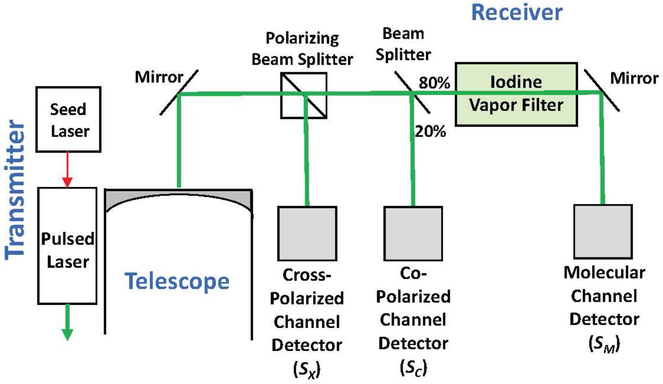
Figure 2. Simplified block diagram of the HSRL-1 instrument deployed on the NASA C-130 aircraft for the NAAMES mission.

The volume depolarization ratio, δ, is the depolarization in the returned signal for all scatterers in the volume (molecules and particles) and is calculated from the ratio of the Cross-Polarized to the Co-Polarized signals at every depth (z):

$$\mathrm{\delta }(z)=\frac{S_X(z)}{S_C(z)}(3)$$

where S_X and S_C are the cross- and co-polarized channel signals. Particulate backscatter, b_bp, at every depth (z) is calculated as follows:

$$b_{bp}\left(z\right)=\chi *{\widehat{\mathrm{\beta }}}_M*\frac{S_C\left(z\right)+S_X\left(z\right)}{S_M\left(z\right)}(4)$$

where S_M is the measured backscatter from water molecules, ${\widehat{\mathrm{\beta }}}_M$ is the 180° backscatter coefficient for seawater (2.45 × 10^–4 m^–1 sr^–1), and χ is the scaling factor from 180° particulate backscatter to hemispheric particulate backscatter and has been set to 0.5 (Hostetler et al., 2018). For both Eqs 3 and 4, the notation has been simplified by assuming that the measured signals have been corrected for differences in optical transmission and electronic gains in the receiver. The diffuse attenuation coefficient at 532 nm (K_d) was calculated as the slope of the co-polarized molecular signal (Hostetler et al., 2018) and used to calculate chlorophyll-a (Chl) concentrations according to Morel et al. (2007).

Backscatter from water molecules is almost entirely parallel to the transmitted pulse, so departure of δ from zero is driven significantly by the depolarization induced by particles. As noted above, depolarization is influenced by changes in PSD, shape, and index of refraction in the single scattering regime, hence changes in δ should provide an indication of changes in particle properties. However, δ also reflects the complicating influence of multiple scattering. Received photons that have undergone more than one scattering event exhibit additional depolarization over singly scattered photons. Higher concentrations of particles give rise to increased multiple scattering and, therefore, increased depolarization (Ivanoff et al., 1961; Loisel et al., 2008; Collister et al., 2018; Liu et al., 2019). The measured volume depolarization therefore depends both on the properties of the particles and their concentration.

Seeking a way to remove the dependence of δ on particle concentration, we focus on the ratio of volume depolarization ratio to particulate backscatter, δ/b_bp, as a parameter that better trends with the depolarization induced by particle properties. Dividing δ by b_bp does not completely remove the impact of multiple scattering since other optical properties, including absorption, impact the scattering signal. However, it does provide a parameter that more directly reflects changes in particle properties by suppressing the impact of changes in concentration and is therefore a potential tool to assess changes in phytoplankton community composition between different water masses.

Satellite Observations and Lagrangian Analysis

We used a combination of satellite observations of sea surface temperature (SST), sea level anomaly (SLA) and geostrophic currents derived from altimetry to help place the ship-based in situ observations into a more regional eddy-wide context. Sea surface temperature observations were downloaded from the GHRSST Level 4 G1SST website². This product, a merge between different satellite observations and data from in situ drifting and moored buoys, is distributed on a daily basis with a spatial resolution of 1 km. Sea level anomaly observations were downloaded from the Copernicus Marine Environment Monitoring Service (CMEMS) and are distributed on a daily basis as 1/4° maps. Ship measurements were collected on November 12, 2015, eleven days prior to the aircraft flight on November 23, 2015. We evaluated whether the water parcel sampled by the ship was comparable to the water mass sampled from the aircraft by estimating maps of origin for water parcels (d’Ovidio et al., 2015; Della Penna and Gaube, 2019). To do this, we downloaded geostrophic currents data from the CMEMS and used the Lagrangian scheme LAMTA to advect water parcels backward in time and identify their spatial origin 15 days previous to the aircraft measurements (Della Penna and Gaube, 2019). The vertical structure in the HSRL data was additionally related to frontal maps derived from the Finite Size Lyapunov Exponents (FSLE). Maps of FSLE, an index of frontal activity and confluence of water parcels, were calculated using LAMTA (d’Ovidio et al., 2015). Details about the method, its limitations and the parameters used for this specific calculation are reported in Della Penna and Gaube (2019).

Results

The SST and SLA fields suggest that the water parcel sampled by the ship and plane was contained within a coherent mesoscale eddy, and remained within this coherent structure over the sampling period (Figures 3a,b). Backtracking of water parcels advected by geostrophic currents indicates that the anticyclonic eddy sampled by the ship and aircraft had been recirculating during the previous several weeks, with only a small contribution of waters coming from roughly 45°S (Figures 3c,d). Even though the altimetry-derived geostrophic currents do not necessarily represent the currents observed within the mixed layer to which the phytoplankton community is constrained, it is reasonable to assume that advective influences were small compared to those outside the eddy and had only a minor impact on community composition, suggesting that the ship-based measurements should be comparable to airborne HSRL data collected 11 days later.

FIGURE 3

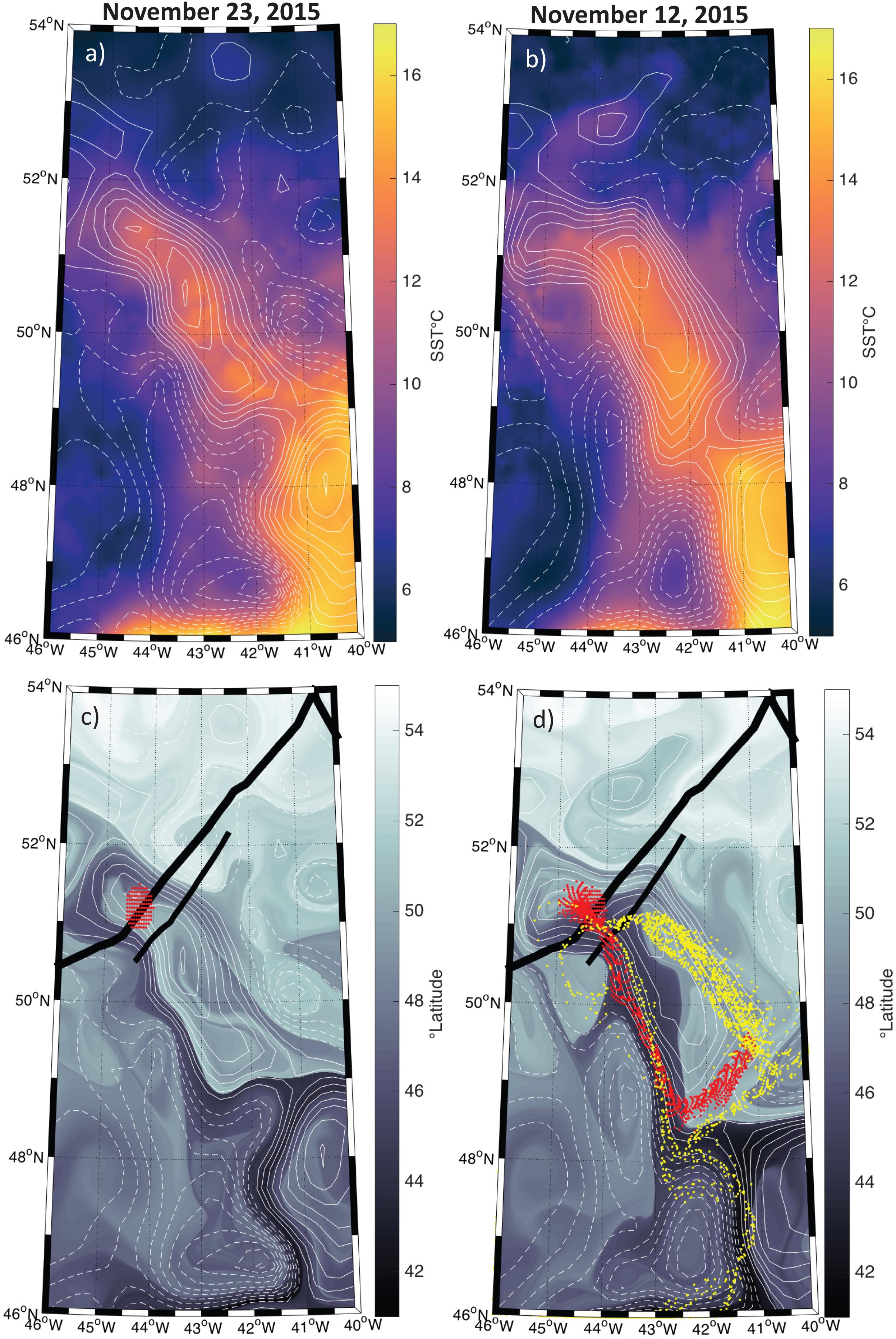
Figure 3. Map of the study region with positive sea level anomalies (SLA) shown in the solid contours and negative anomalies shown in the hashed contours at an interval of 5 cm. (a) Sea surface temperature (SST) on November 23, 2015 from the MUR SST product. (b) Same as (a) but for November 12, 2015. (c) The latitudinal orgin of each water parcel 15 days prior to November 23, 2015. Thick and thin black lines indicate the airplaine and ship tracks, respectively. Dots represent passive tracers advected using the Lagrangian routine described in the methods section with a start data of November 23, 2015. (d) Same as (c) but for November 12, 2015. The red dots in both panels (c,d) represent the particles backtracked from November 23, 2015 and ending on November 12, 2015. Yellow dots in panel (d) represent the particles backtracked from November 12, 2015 to October 22, 2015.

Salinity and temperature were elevated inside the eddy when compared to measurements made outside the eddy (Figure 4a). Phytoplankton biomass (assumed to scale linearly with b_bp) and chlorophyll-a were highly correlated, with both properties having lower values inside the eddy (Figure 4b). Cell shape and size measurements from the IFCB and the optically-based estimate of the size index parameter (γ) revealed that particles were smaller and more eccentric inside the eddy (Figure 4c).

FIGURE 4

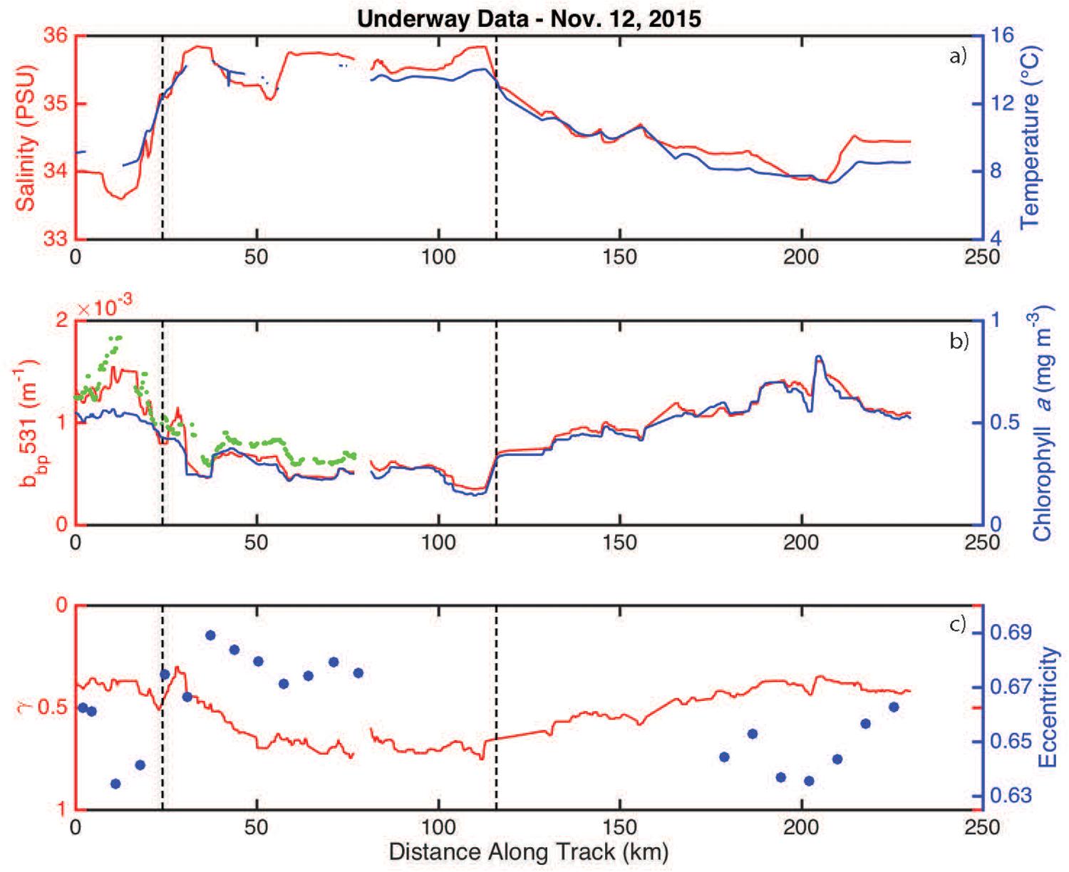
Figure 4. Underway measurements collected along the November 12, 2015 ship track. (a) Salinity and temperature are shown in red and blue, respectively. The eddy boundaries (defined using the derivative of b_bp) are indicated by the vertical hashed lines. (b) b_bp and chlorophyll-a concentrations are shown in red and blue, respectively. The green dots are the available ECO-BB3 measurements. (c) The size index parameter (γ) and average particle eccentricity are shown in red and blue, respectively.

Imaging flow cytobot data show that cell abundances for all phytoplankton groups (>8 μm) decreased inside the eddy (Figure 5), with the largest decrease observed for dinoflagellates. Dinoflagellates (all groups), on average, accounted for 25% of the total phytoplankton community outside the eddy and 16% inside the eddy. Cells of the class Dinophyceae (mean equivalent sphere diameter ($\overline{x}$_{rm ESD}) = 10.6 ± 2.8 μm) decreased from an average of 22 cells mL^–1 outside the eddy compared to ∼4 cells mL^–1 inside the eddy. Additionally, smaller dinoflagellates of the genus Oxytoxum ($\overline{x}$_{rm ESD} = 8.5 ± 1.1 μm) decreased from an average concentration of ∼7 cells mL^–1 outside the eddy to concentrations that were too low to report with confidence (∼1 cell mL^–1) inside the eddy. Less than ten large dinoflagellate cells (>20 μm) total were present in samples from within the eddy. However, statistical counting errors of rarely observed cells are relatively high.

FIGURE 5

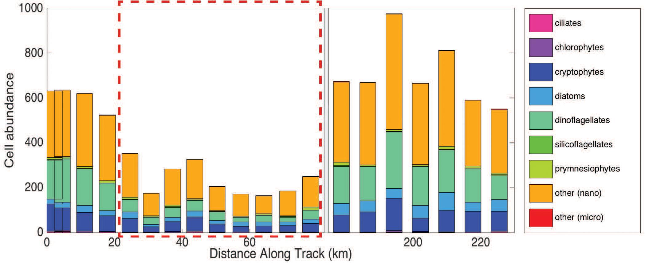
Figure 5. Group-specific cell abundance per 5 mL sample for each station measured using the Imaging Flow Cytobot (IFCB). There is a break in the x-axis from 80 to 175 km (instrument was diverted from the in-line system). The hashed red box denotes the samples collected in the eddy core.

Influx Cell Sorter data show decreased abundances of Synechococcus spp. and nanoeukaryotes inside the eddy compared to outside, while picoeukaryotes decreased from north to south (Table 1). The most significant change was the reduction in nanoeukaryotes and larger cells inside of the eddy, consistent with the IFCB results for this narrow phytoplankton size range where these two instrument measurements overlap. Mean cellular FSC (except for Synechococcus spp.) and SSC were lower inside the eddy, though the change was much greater in the SSC channel (Table 1). The mean SSC more than doubled for pico- and nanoeukaryotes outside of the eddy compared to inside, suggesting a change in community structure, size, and/or cellular composition within phytoplankton groups that are below the detection limit of the IFCB.

TABLE 1

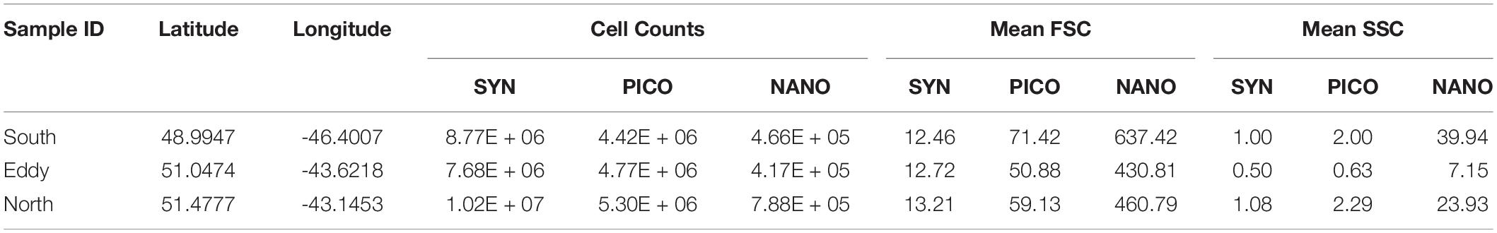
Table 1. Cell counts, forward scatter (FSC) and side scatter (SSC) properties measured from the ICS for Synechococcus spp. (SYN), picoeukaryotes (PICO) and nanoeukaryotes (NANO).

High spectral resolution lidar b_bp values were lower inside the eddy with sharp gradients observed along the eddy periphery (Figure 6a). The gradients along the north side of the eddy are weaker than those to the south, likely due to enhanced mixing along the northern front. The depolarization ratio was lower inside the eddy (Figure 6b) and was correlated with b_bp for measurements collected both inside (R² = 0.77; p < 0.001) and outside the eddy (R² = 0.89; p < 0.001). The ratio, δ/b_bp, was 15% greater inside the eddy (Figure 6c). Linear models were fit to b_bp and δ for both water types (i.e., eddy, outside eddy) for data collected between 5 and 15 m (Figure 7A). This depth range was chosen to eliminate surface effects (e.g., bubbles) and maximize the signal-to-noise ratio of the data analyzed. Data collected from 115 to 150 km along track (between the red and yellow arrows in Figure 6) were excluded from the analysis since this region contains water characteristic of inside and outside the eddy. Over the full data range measured by the HSRL, the relationship between b_bp and δ is linear at low b_bp and asymptotes at higher values (Figure 7B). The dynamic range for the data presented in this study is much narrower than the dynamic range encountered in September 2017 (Figure 7B). This is because the non-blooming phase of the annual phytoplankton bloom cycle occurs in November, while in September, ecological processes have acted in different ways resulting in greater spatiotemporal variability in phytoplankton biomass. However, the general shape of this relationship is consistent across all ocean waters with the slope, δ/b_bp, changing between water masses. We attribute the slope differences (changes in δ/b_bp) to changes in the optical properties of the bulk particle assemblage.

FIGURE 6

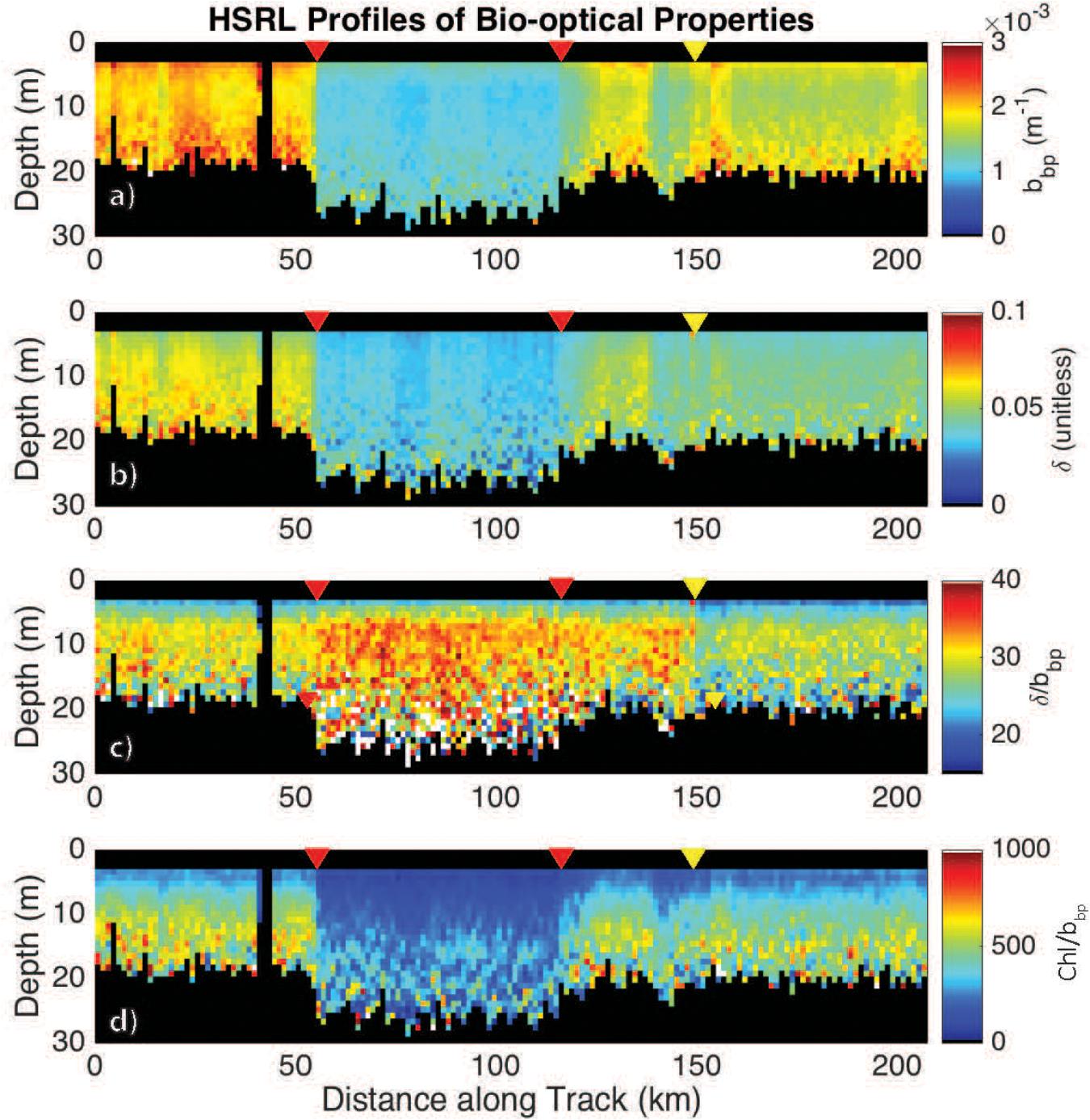
Figure 6. HSRL measurements of (a) b_bp, m^–1; (b) the depolarization ratio, δ (unitless); (c) the ratio δ/b_bp; and (d) the Chl:b_bp ratio across the eddy. The red triangles mark the eddy core boundaries. The yellow triangle marks the boundary in the ratio, b_bp/δ. Chl was calculated as a function of K_d following Morel et al. (2007).

FIGURE 7

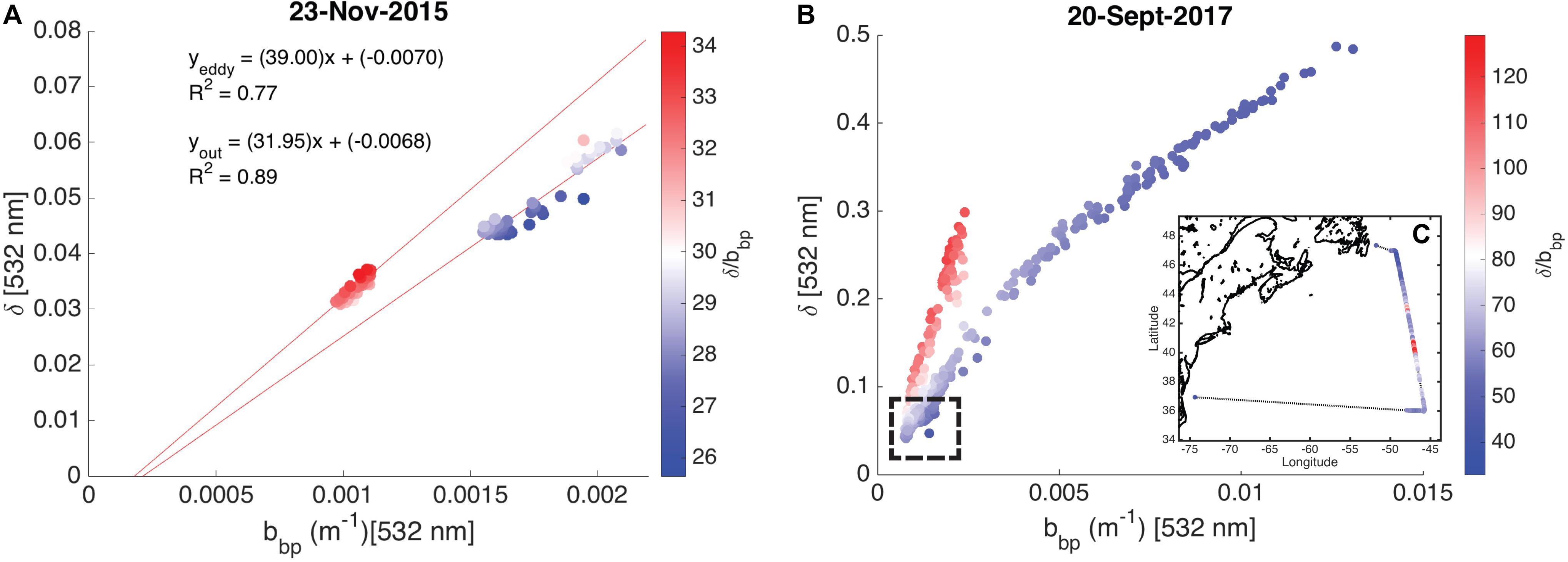
Figure 7. Scatter plots showing the relationship between the particulate backscattering coefficient (b_bp, m^–1) and the depolarization ratio (δ, unitless) shown as a function of the ratio, δ/b_bp. (A) Measurements collected on November 23, 2015 (data presented in this study) are shown. The linear models for data collected inside and outside the eddy are presented with R² values. (B) Measurements collected on September 20, 2017 are shown. No in situ data are available for this flight. The hashed box shows the dynamic range of data presented in this study. (C) The inset shows δ/b_bp along the entire September 20, 2017 flight line.

Additional support showing that the ratio, δ/b_bp, is tracking changes in phytoplankton community composition is the twofold decrease in the Chl:b_bp ratio inside the eddy (Figure 6d). This ratio has previously been used an optical index for tracking changes in phytoplankton community composition (Cetinić et al., 2015; Lacour et al., 2019), though can also be impacted by the photoacclimation state of the cells (Behrenfeld et al., 2016).

The boundaries observed in lidar-retrieved properties are spatially coincident with geostrophically-driven frontal regions calculated from FSLE (Figure 8). The northern boundary in the ratio, δ/b_bp, shifted to ∼150 km along track, which corresponds to another frontal feature highlighted as a ridge of FSLE (Figure 8). The vertically-resolved lidar measurements highlight an abrupt boundary (indicated by the triangles in Figure 6) between water masses within the mixed layer (estimated at ∼100 m; Mojica and Gaube, Submitted Journal of Marine Systems). Further, these measurements reveal vertical heterogeneity of phytoplankton within the mixed layer. This is particularly evident in the strata between 9 and 15 m depth where the low b_bp values extend further along the track when compared to the near-surface layer (3–7 m).

FIGURE 8

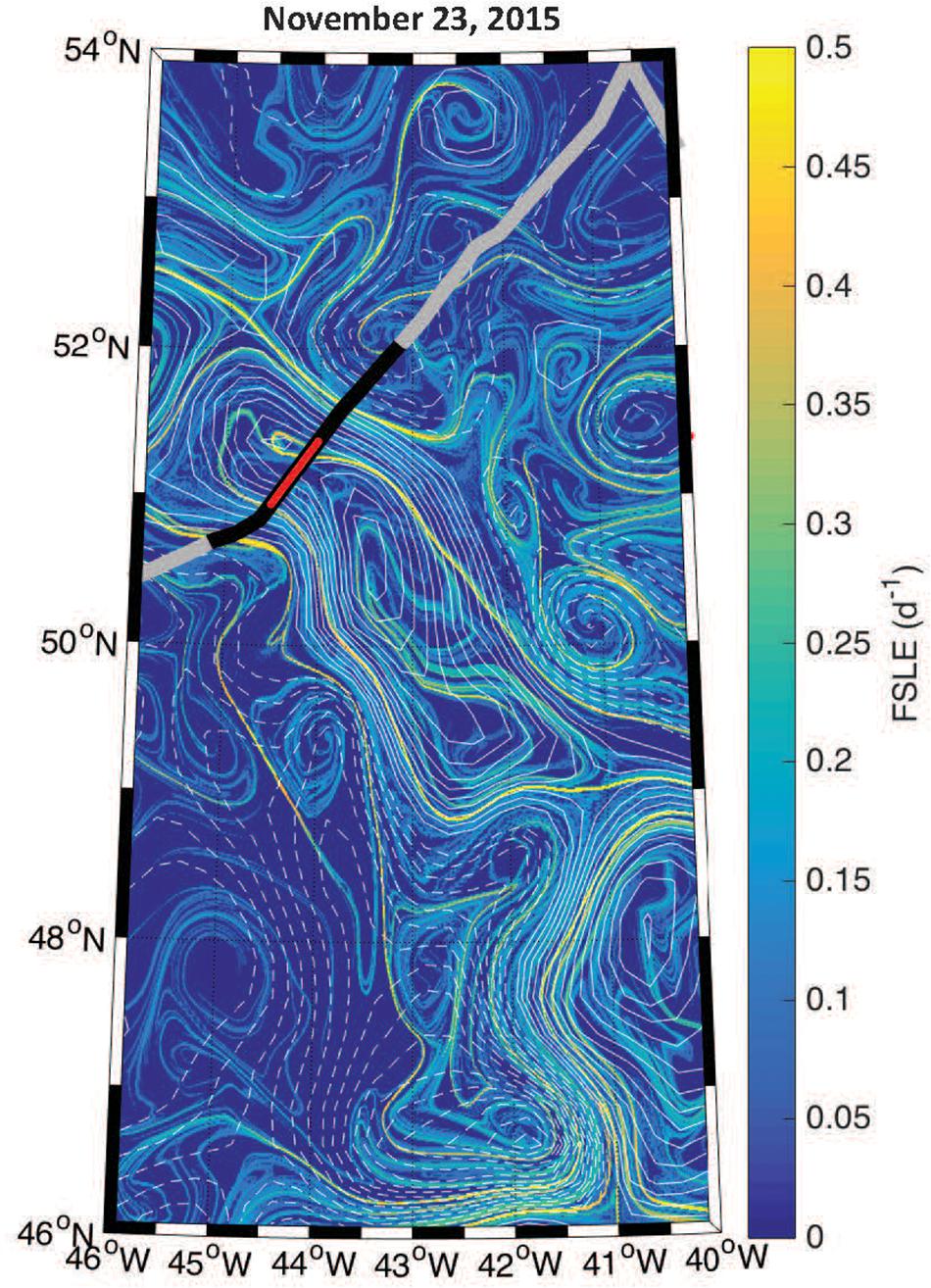
Figure 8. Geostrophic fronts derived from the Finite Size Lyapunov Exponents (FSLE) overlaid with contours of SLA (solid and dashed contours of positive and negative SLA, respectively, at an interval of 3 cm). The thick black line corresponds to the segment of the flight track shown in Figure 6 and the red line shows the eddy core.

Discussion

This is the first study illustrating the use of HSRL measurements of δ, b_bp, and K_d in detecting changes in phytoplankton assemblages along an environmental gradient. The increase in δ/b_bp inside the warm and saline anticyclonic eddy coincided with a twofold decrease in Chl:b_bp, providing further evidence that the changes observed in HSRL bio-optical properties were being driven by changes in phytoplankton community composition. Phytoplankton cells were smaller and less spherical in shape. Biomass was lower inside the eddy and there was a significant decrease in the relative abundance of dinoflagellates. Dinoflagellates have a unique cellular structure among phytoplankton, giving this group a higher refractive index relative to other phytoplankton classes, except for coccolithophorids (Aas, 1981), which were not observed in our samples. Dinoflagellates have high internal cellular carbon content compared to other phytoplankton groups (Vaillancourt et al., 2004) and a unique internal structure, including specialized vacuoles called pusules (Dodge, 1972; Graham and Wilcox, 2000) and a highly condensed nucleus (Bhaud et al., 2000), which all contribute to this group having a high refractive index compared to other phytoplankton groups. We would thus predict a decrease in the bulk index of refraction inside the eddy resulting from the threefold reduction in this group, assuming no change in the composition or the proportion of non-living particles. Significant variability in backscattering within and among species exists, so the role of the refractive index in driving the scattering signal could not be evaluated directly in this study.

Assuming a reduction in the bulk index of refraction resulting from the observed relative decrease in dinoflagellates, Lorenz-Mie theory predicts a negative change in depolarization, which is opposite to the pattern observed here. Also inconsistent with theory, the IFCB, flow cytometer, and γ calculated from spectral c_p (See Eq. 1), all indicate a shift to smaller cells inside the eddy. These results suggest that the depolarization ratio at 180° is potentially most sensitive to changes in cell shape over the range of cell types observed during the sampling period. Voss and Fry (1984) measured depolarization (10°–160°) for optically diverse ocean waters (over 200 Mueller matrices measured) and found cell shape deviations from sphericity resulted in depolarization. Fry and Voss (1985) and Quinby-Hunt et al. (1989) measured Mueller matrices (near 180°) from phytoplankton cultures and also found depolarization measurements sensitive to changes in cell shape. Our results are consistent with these findings, such that the relative decrease in spherical dinoflagellates inside the eddy resulted in a greater proportion of non-spherical cells.

Dinoflagellates are notoriously difficult to identify using ocean color data alone because of their overlapping pigment and size distributions with other phytoplankton groups (Dierssen et al., 2006; Mouw et al., 2017), although some regional algorithms developed using absorption and scattering data have been applied in the context of HABs (Cannizzaro et al., 2008; Tomlinson et al., 2009; Palacios et al., 2015). The ability to relate lidar-retrieved properties to changes in dinoflagellate abundance is encouraging for future studies of this ecologically important group of phytoplankton (Smayda, 1997; Hinder et al., 2012).

In addition to community changes identified by IFCB for larger phytoplankton, ICS data documented a clear shift in contributions from Synechococcus spp., picoeukaryotes, and nanoeukaryotes. Mean SSC, a measure of cellular complexity/structure (Moutier et al., 2017 and references therein), was significantly lower inside the eddy compared to outside. Using a coated-sphere model and in situ optical measurements, Organelli et al. (2018) show that 50% of backscattered signal comes from particles 3–4 μm in diameter, indicating that changes in these groups also contribute to the observed the δ/b_bp variability. Additional research will be needed to further understand how the smaller phytoplankton groups impact the HSRL-retrieved scattering properties.

Our primary hypothesis was that δ/b_bp tracks changes in particulate depolarization that are related to phytoplankton cell properties. An alternative explanation for the consistency between observed changes in community composition with changes δ/b_bp is that the ensemble particle phase function varies with community composition. For instance, Collister et al. (2018) reported a strong correlation of lidar depolarization with in situ observations of b_bp/b_p and attributed variation in the latter to differences in particle composition. Their study, however, concerned a different formulation of lidar depolarization (i.e., cross-polarized signal/total signal) from a ship-based elastic backscatter lidar. It is also possible that the changes observed in δ/b_bp could be due to changes in composition or proportion of non-living particles. However, the consistency of the NAAMES airborne HSRL results with in situ observations builds confidence that the lidar observations of δ/b_bp do indeed track changes in community composition.

Looking at the transect data as a whole, a significant feature in the HSRL profiles is the abrupt transitions in water properties at the eddy boundaries. These observations highlight how mesoscale eddies can generate abrupt changes in the near-surface optical properties. Further, these gradients were spatially coincident with frontal regions calculated from geostrophic currents. This implies, to first order, that fronts in the vertically-integrated geostrophic velocity field correspond to abrupt changes in the lidar-retrieved properties in the top 2.5 optical depths. This is encouraging for the application of geostrophic velocity data to define boundaries of different biological regimes, which is somewhat surprising as these currents do not include the effect of wind, waves, and small-scale processes. Finally, it must be noted that such subsurface structure in phytoplankton biomass cannot be detected using contemporary passive satellite remote sensing techniques.

The results of this study demonstrate that airborne HSRL measurements of δ and b_bp track changes in phytoplankton community composition and that this signal is potentially most sensitive to changes in phytoplankton shape. While additional research is needed to address some of the interpretations discussed here, this study represents a significant step forward in adding scientific relevance to satellite lidar observations. This study is contributing to a series of documented advantages of lidar measurements that have led to a greater understanding of ocean biological processes and biogeochemistry (Behrenfeld et al., 2017, 2019a; Schulien et al., 2017).

Data Availability Statement

The datasets generated for this study can be found in SeaBASS (NAAMES SeaBASS). DOI: 10.5067/SeaBASS/NAAMES/DATA001.

Author Contributions

JS and AD led the writing of the manuscript. All authors provided figures, data, text, and/or comments for the manuscript and/or played leading roles in the data collection.

Funding

This study was supported by the NASA NAAMES project award NNX15AF30G and NASA award NNX15AI15G. PG acknowledges the support of NASA award 80NSSC18K0199 and NSF award OCE-1558809. AD is grateful for the support of the Applied Physics Laboratory Science and Engineering Enrichment Development (SEED) fellowship and the European Union’s Horizon 2020 Research and Innovation Program under the Marie Sklodowska-Curie grant agreement No. 749591.

Conflict of Interest

The authors declare that the research was conducted in the absence of any commercial or financial relationships that could be construed as a potential conflict of interest.

The reviewer GD declared a past co-authorship with several of the authors EB, MB, JG, AC, JH, and CH to the handling Editor.

Acknowledgments

We utilized and acknowledge E.U. Copernicus Marine Service Information (CMEMS). We also gratefully acknowledge the captain and crew of the R/V Atlantis and the support of St. John’s International Airport.

Footnotes

1. ^ https://github.com/hsosik/ifcb-analysis/wiki
2. ^ https://podaac.jpl.nasa.gov/dataset/JPL_OUROCEAN-L4UHfnd-GLOB-G1SST

References

Aas, E. (1981). The Refractive Index of Phytoplankton. Oslo: Universitetet i Oslo.

Google Scholar

Anderson, C. R., Siegel, D. A., Brzezinski, M. A., and Guillocheau, N. (2008). Controls on temporal patterns in phytoplankton community structure in the Santa Barbara Channel, California. J. Geophys. Res. Oceans 113:C04038.

Google Scholar

Behrenfeld, M. J., Gaube, P., Della Penna, A., O’Malley, R. T., Burt, W. J., Hu, Y., et al. (2019a). Satellite-observed daily vertical migrations of global ocean animals. Nature 576, 257–261. doi: 10.1038/s41586-019-1796-9

PubMed Abstract | CrossRef Full Text | Google Scholar

Behrenfeld, M. J., Hu, Y., O’Malley, R. T., Boss, E. S., Hostetler, C. A., Siegel, D. A., et al. (2017). Annual boom–bust cycles of polar phytoplankton biomass revealed by space-based lidar. Nat. Geosci. 10:118. doi: 10.1038/ngeo2861

CrossRef Full Text | Google Scholar

Behrenfeld, M. J., Moore, R. H., Hostetler, C. A., Graff, J., Gaube, P., Russell, L. M., et al. (2019b). The North Atlantic aerosol and marine ecosystem Study (NAAMES): science motive and mission overview. Front. Mar. Sci. 6:122. doi: 10.3389/fmars.2019.00122

CrossRef Full Text | Google Scholar

Behrenfeld, M. J., O’Malley, R. T., Boss, E. S., Westberry, T. K., Graff, J. R., Halsey, K. H., et al. (2016). Revaluating ocean warming impacts on global phytoplankton. Nat. Clim. Change 6, 323–330. doi: 10.1038/nclimate2838

CrossRef Full Text | Google Scholar

Bhaud, Y., Guillebault, D., Lennon, J., Defacque, H., Soyer-Gobillard, M. O., and Moreau, H. (2000). Morphology and behaviour of dinoflagellate chromosomes during the cell cycle and mitosis”. J. Cell Sci. 113(Pt 7), 1231–1239.

Google Scholar

Cannizzaro, J. P., Carder, K. L., Chen, F. R., Heil, C. A., and Vargo, G. A. (2008). A novel technique for detection of the toxic dinoflagellate, Karenia brevis, in the Gulf of Mexico from remotely sensed ocean color data. Continent. Shelf Res. 28, 137–158. doi: 10.1016/j.csr.2004.04.007

CrossRef Full Text | Google Scholar

Cetinić, I., Perry, M. J., D’asaro, E., Briggs, N., Poulton, N., Sieracki, M. E., et al. (2015). A simple optical index shows spatial and temporal heterogeneity in phytoplankton community composition during the 2008 North Atlantic Bloom experiment. Biogeosciences 12, 2179–2194. doi: 10.5194/bg-12-2179-2015

CrossRef Full Text | Google Scholar

Chami, M., and McKee, D. (2007). Determination of biogeochemical properties of marine particles using above water measurements of the degree of polarization at the Brewster angle. Opt. Express 15, 9494–9509.

Google Scholar

Chelton, D. B., Gaube, P., Schlax, M. G., Early, J. J., and Samelson, R. M. (2011). The influence of nonlinear mesoscale eddies on near-surface oceanic chlorophyll. Science 334, 328–332. doi: 10.1126/science.1208897

PubMed Abstract | CrossRef Full Text | Google Scholar

Collister, B. L., Zimmerman, R. C., Sukenik, C. I., Hill, V. J., and Balch, W. M. (2018). Remote sensing of optical characteristics and particle distributions of the upper ocean using shipboard lidar. Remote Sens. Environ. 215, 85–96. doi: 10.1016/j.rse.2018.05.032

CrossRef Full Text | Google Scholar

Dandonneau, Y., Deschamps, P. Y., Nicolas, J. M., Loisel, H., Blanchot, J., Montel, Y., et al. (2004). Seasonal and interannual variability of ocean color and composition of phytoplankton communities in the North Atlantic, equatorial Pacific and South Pacific. Deep Sea Res. II Top. Stud. Oceanogr. 51, 303–318. doi: 10.1016/j.dsr2.2003.07.018

CrossRef Full Text | Google Scholar

Della Penna, A., and Gaube, P. (2019). Overview of (Sub) mesoscale ocean dynamics for the NAAMES field program. Front. Mar. Sci. 6:384. doi: 10.3389/fmars.2019.00384

CrossRef Full Text | Google Scholar

Dierssen, H. M., Kudela, R. M., Ryan, J. P., and Zimmerman, R. C. (2006). Red and black tides: quantitative analysis of water-leaving radiance and perceived color for phytoplankton, colored dissolved organic matter, and suspended sediments. Limnol. Oceanogr. 51, 2646–2659. doi: 10.4319/lo.2006.51.6.2646

CrossRef Full Text | Google Scholar

Dodge, J. D. (1972). The ultrastructure of the dinoflagellate pusule: a unique osmo-regulatory organelle. Protoplasma 75, 285–302. doi: 10.1007/bf01279820

CrossRef Full Text | Google Scholar

d’Ovidio, F., Della Penna, A., Trull, T. W., Nencioli, F., Pujol, M. I., Rio, M. H., et al. (2015). The biogeochemical structuring role of horizontal stirring: lagrangian perspectives on iron delivery downstream of the Kerguelen plateau. Biogeosciences 12, 5567–5581. doi: 10.5194/bg-12-5567-2015

CrossRef Full Text | Google Scholar

Dufois, F., Hardman-Mountford, N. J., Greenwood, J., Richardson, A. J., Feng, M., Herbette, S., et al. (2014). Impact of eddies on surface chlorophyll in the South Indian Ocean. J. Geophys. Res. Oceans 119, 8061–8077. doi: 10.1002/2014jc010164

CrossRef Full Text | Google Scholar

Falkowski, P. G., Algeo, T., Codispoti, L., Deutsch, C., Emerson, S., Hales, B., et al. (2011). Ocean deoxygenation: past, present, and future. EOS Trans. Am. Geophys. Union 92, 409–410.

Google Scholar

Fournier, G., and Neukermans, G. (2017). An analytical model for light backscattering by coccoliths and coccospheres of Emiliania huxleyi. Opt. Express 25, 14996–15009. doi: 10.1364/OE.25.014996

PubMed Abstract | CrossRef Full Text | Google Scholar

Fry, E. S., and Voss, K. J. (1985). Measurement of the Mueller matrix for phytoplankton1. Limnol. Oceanogr. 30, 1322–1326. doi: 10.4319/lo.1985.30.6.1322

CrossRef Full Text | Google Scholar

Gaube, P., Chelton, D. B., Samelson, R. M., Schlax, M. G., and O’Neill, L. W. (2015). Satellite observations of mesoscale eddy-induced Ekman pumping. J. Phys. Oceanogr. 45, 104–132. doi: 10.1175/jpo-d-14-0032.1

CrossRef Full Text | Google Scholar

Gaube, P., Chickadel, C. C., Branch, R., and Jessup, A. (2019). Satellite observations of SST-induced wind speed perturbation at the oceanic submesoscale. Geophys. Res. Lett. 46, 2690–2695. doi: 10.1029/2018gl080807

CrossRef Full Text | Google Scholar

Gaube, P., and McGillicuddy, D. J. Jr. (2017). The influence of Gulf Stream eddies and meanders on near-surface chlorophyll. Deep Sea Res. I Oceanogr. Res. Pap. 122, 1–16. doi: 10.1016/j.dsr.2017.02.006

CrossRef Full Text | Google Scholar

Gaube, P., McGillicuddy, D. J. Jr., Chelton, D. B., Behrenfeld, M. J., and Strutton, P. G. (2014). Regional variations in the influence of mesoscale eddies on near-surface chlorophyll. J. Geophys. Res. Oceans 119, 8195–8220. doi: 10.1002/2014jc010111

CrossRef Full Text | Google Scholar

Graff, J. R., and Behrenfeld, M. J. (2018). Photoacclimation responses in subarctic atlantic phytoplankton following a natural mixing-restratification event. Front. Mar. Sci. 5:209. doi: 10.3389/fmars.2018.00209

CrossRef Full Text | Google Scholar

Graff, J. R., Westberry, T. K., Milligan, A. J., Brown, M. B., Dall’Olmo, G., van Dongen-Vogels, V., et al. (2015). Analytical phytoplankton carbon measurements spanning diverse ecosystems. Deep Sea Res. I Oceanogr. Res. Pap. 102, 16–25. doi: 10.1016/j.dsr.2015.04.006

CrossRef Full Text | Google Scholar

Graham, L. E., and Wilcox, L. W. (2000). Algae. Upper Saddle River: Prentice Hall.

Google Scholar

Hair, J., Hostetler, C., Hu, Y., Behrenfeld, M., Butler, C., Harper, D., et al. (2016). “Combined atmospheric and ocean profiling from an airborne high spectral resolution lidar,” in Proceedings of the EPJ Web of Conferences, Vol. 119, (Les Ulis: EDP Sciences), 22001. doi: 10.1051/epjconf/201611922001

CrossRef Full Text | Google Scholar

Hair, J. W., Hostetler, C. A., Cook, A. L., Harper, D. B., Ferrare, R. A., Mack, T. L., et al. (2008). Airborne high spectral resolution lidar for profiling aerosol optical properties. Appl. Opt. 47, 6734–6752.

Google Scholar

Hinder, S. L., Hays, G. C., Edwards, M., Roberts, E. C., Walne, A. W., and Gravenor, M. B. (2012). Changes in marine dinoflagellate and diatom abundance under climate change. Nat. Clim. Change 2:271. doi: 10.1038/nclimate1388

CrossRef Full Text | Google Scholar

Hood, R. R., Laws, E. A., Armstrong, R. A., Bates, N. R., Brown, C. W., Carlson, C. A., et al. (2006). Pelagic functional group modeling: progress, challenges and prospects. Deep Sea Res. II Top. Stud. Oceanogr. 53, 459–512.

Google Scholar

Hostetler, C. A., Behrenfeld, M. J., Hu, Y., Hair, J. W., and Schulien, J. A. (2018). Spaceborne lidar in the study of marine systems. Annu. Rev. Mar. Sci. 10, 121–147. doi: 10.1146/annurev-marine-121916-063335

PubMed Abstract | CrossRef Full Text | Google Scholar

Ivanoff, A., Jerlov, N., and Waterman, T. H. (1961). A comparative study of irradiance, beam transmittance and scattering in the sea near bermuda 1. Limnol. Oceanogr. 6, 129–148. doi: 10.4319/lo.1961.6.2.0129

CrossRef Full Text | Google Scholar

Kostadinov, T. S., Siegel, D. A., and Maritorena, S. (2010). Global variability of phytoplankton functional types from space: assessment via the particle size distribution. Biogeosciences 7, 3239–3257. doi: 10.5194/bg-7-3239-2010

CrossRef Full Text | Google Scholar

Lacour, L., Briggs, N., Claustre, H., Ardyna, M., and Dall’Olmo, G. (2019). The intraseasonal dynamics of the mixed layer pump in the subpolar North Atlantic Ocean: a biogeochemical-argo float approach. Glob. Biogeochem. Cycles 33, 266–281. doi: 10.1029/2018gb005997

CrossRef Full Text | Google Scholar

Lehahn, Y., d’Ovidio, F., Lévy, M., Amitai, Y., and Heifetz, E. (2011). Long range transport of a quasi isolated chlorophyll patch by an Agulhas ring. Geophys. Res. Lett. 38:L16610.

Google Scholar

Liu, Q., Cui, X., Chen, W., Liu, C., Bai, J., Zhang, Y., et al. (2019). A semianalytic Monte Carlo radiative transfer model for polarized oceanic lidar: experiment-based comparisons and multiple scattering effects analyses. J. Quant. Spectrosc. Radiat. Transf. 237;106638. doi: 10.1016/j.jqsrt.2019.106638

CrossRef Full Text | Google Scholar

Loisel, H., Duforet, L., Dessailly, D., Chami, M., and Dubuisson, P. (2008). Investigation of the variations in the water leaving polarized reflectance from the POLDER satellite data over two biogeochemical contrasted oceanic areas. Opt. Express 16, 12905–12918.

Google Scholar

Lotsberg, J. K., and Stamnes, J. J. (2010). Impact of particulate oceanic composition on the radiance and polarization of underwater and backscattered light. Opt. Express 18, 10432–10445.

Google Scholar

McGillicuddy, D. J., Anderson, L. A., Bates, N. R., Bibby, T., Buesseler, K. O., Carlson, C. A., et al. (2007). Eddy/wind interactions stimulate extraordinary mid-ocean plankton blooms. Science 316, 1021–1026. doi: 10.1126/science.1136256

PubMed Abstract | CrossRef Full Text | Google Scholar

Mishchenko, M. I., and Travis, L. D. (1998). Capabilities and limitations of a current FORTRAN implementation of the T-matrix method for randomly oriented, rotationally symmetric scatterers. J. Quant. Spectrosc. Radiat. Transf. 60, 309–324. doi: 10.1016/s0022-4073(98)00008-9

CrossRef Full Text | Google Scholar

Morel, A., Huot, Y., Gentili, B., Werdell, P. J., Hooker, S. B., and Franz, B. A. (2007). Examining the consistency of products derived from various ocean color sensors in open ocean (Case 1) waters in the perspective of a multi-sensor approach. Remote Sens. Environ. 111, 69–88. doi: 10.1016/j.rse.2007.03.012

CrossRef Full Text | Google Scholar

Moutier, W., Duforêt-Gaurier, L., Thyssen, M., Loisel, H., Meriaux, X., Courcot, L., et al. (2017). Evolution of the scattering properties of phytoplankton cells from flow cytometry measurements. PLoS One 12:e0181180. doi: 10.1371/journal.pone.0181180

PubMed Abstract | CrossRef Full Text | Google Scholar

Mouw, C. B., Hardman-Mountford, N. J., Alvain, S., Bracher, A., Brewin, R. J., Bricaud, A., et al. (2017). A consumer’s guide to satellite remote sensing of multiple phytoplankton groups in the global ocean. Front. Mar. Sci. 4:41. doi: 10.3389/fmars.2017.00041

CrossRef Full Text | Google Scholar

Organelli, E., Dall’Olmo, G., Brewin, R. J., Tarran, G. A., Boss, E., and Bricaud, A. (2018). The open-ocean missing backscattering is in the structural complexity of particles. Nat. Commun. 9:5439.

Google Scholar

Palacios, S. L., Kudela, R. M., Guild, L. S., Negrey, K. H., Torres-Perez, J., and Broughton, J. (2015). Remote sensing of phytoplankton functional types in the coastal ocean from the HyspIRI preparatory flight campaign. Remote Sens. Environ. 167, 269–280. doi: 10.1016/j.rse.2015.05.014

CrossRef Full Text | Google Scholar

Picheral, M., Colin, S., and Irisson, J.-O. (2017). EcoTaxa, A Tool for the Taxonomic Classification of Images. Available online at: http://ecotaxa.obs-vlfr.fr (accessed July 30, 2019).

Google Scholar

Quinby-Hunt, M. S., Hunt, A. J., Lofftus, K., and Shapiro, D. (1989). Polarized-light scattering studies of marine Chlorella. Limnol. Oceanogr. 34, 1587–1600. doi: 10.4319/lo.1989.34.8.1587

CrossRef Full Text | Google Scholar

Richardson, T. L., and Jackson, G. A. (2007). Small phytoplankton and carbon export from the surface ocean. Science 315, 838–840. doi: 10.1126/science.1133471

PubMed Abstract | CrossRef Full Text | Google Scholar

Schulien, J. A., Behrenfeld, M. J., Hair, J. W., Hostetler, C. A., and Twardowski, M. S. (2017). Vertically-resolved phytoplankton carbon and net primary production from a high spectral resolution lidar. Opt. Express 25, 13577–13587.

Google Scholar

Sieracki, M., and Poulton, N. (2011). The 2008 North Atlantic Bloom Experiment Abundance and Biomass Determination of Heterotrophic and Autotrophic Bacteria, Phototrophic and Heterotrophic Nanoplankton, & Microplankton-Including Instrument Calibrationversion 1.3.

Google Scholar

Slade, W. H., Boss, E., Dall’Olmo, G., Langner, M. R., Loftin, J., Behrenfeld, M. J., et al. (2010). Underway and moored methods for improving accuracy in measurement of spectral particulate absorption and attenuation. J. Atmos. Ocean. Technol. 27, 1733–1746. doi: 10.1175/2010jtecho755.1

CrossRef Full Text | Google Scholar

Smayda, T. J. (1997). Harmful algal blooms: their ecophysiology and general relevance to phytoplankton blooms in the sea. Limnol. Oceanogr. 42(Pt 2), 1137–1153. doi: 10.4319/lo.1997.42.5_part_2.1137

CrossRef Full Text | Google Scholar

Sosik, H. M., and Olson, R. J. (2007). Automated taxonomic classification of phytoplankton sampled with imaging-in-flow cytometry. Limnol. Oceanogr. Methods 5, 204–216. doi: 10.4319/lom.2007.5.204

CrossRef Full Text | Google Scholar

Tomlinson, M. C., Wynne, T. T., and Stumpf, R. P. (2009). An evaluation of remote sensing techniques for enhanced detection of the toxic dinoflagellate, Karenia brevis. Remote Sens. Environ. 113, 598–609. doi: 10.1016/j.rse.2008.11.003

CrossRef Full Text | Google Scholar

Uitz, J., Claustre, H., Gentili, B., and Stramski, D. (2010). Phytoplankton class-specific primary production in the world’s oceans: seasonal and interannual variability from satellite observations. Glob. Biogeochem. Cycles 24:GB3016.

Google Scholar

Uitz, J., Stramski, D., Reynolds, R. A., and Dubranna, J. (2015). Assessing phytoplankton community composition from hyperspectral measurements of phytoplankton absorption coefficient and remote-sensing reflectance in open-ocean environments. Remote Sens. Environ. 171, 58–74. doi: 10.1016/j.rse.2015.09.027

CrossRef Full Text | Google Scholar

Vaillancourt, R. D., Brown, C. W., Guillard, R. R., and Balch, W. M. (2004). Light backscattering properties of marine phytoplankton: relationships to cell size, chemical composition and taxonomy. J. Plankton Res. 26, 191–212. doi: 10.1093/plankt/fbh012

CrossRef Full Text | Google Scholar

Vaillancourt, R. D., Marra, J., Seki, M. P., Parsons, M. L., and Bidigare, R. R. (2003). Impact of a cyclonic eddy on phytoplankton community structure and photosynthetic competency in the subtropical North Pacific Ocean. Deep Sea Res. I Oceanogr. Res. Pap. 50, 829–847. doi: 10.1016/s0967-0637(03)00059-1

CrossRef Full Text | Google Scholar

Volten, H., De Haan, J. F., Hovenier, J. W., Schreurs, R., Vassen, W., Dekker, A. G., et al. (1998). Laboratory measurements of angular distributions of light scattered by phytoplankton and silt. Limnol. Oceanogr. 43, 1180–1197. doi: 10.4319/lo.1998.43.6.1180

CrossRef Full Text | Google Scholar

Voss, K. J., and Fry, E. S. (1984). Measurement of the Mueller matrix for ocean water. Appl. Opt. 23, 4427–4439.

Google Scholar

Werdell, P. J., Roesler, C. S., and Goes, J. I. (2014). Discrimination of phytoplankton functional groups using an ocean reflectance inversion model. Appl. Opt. 53, 4833–4849.

Google Scholar