The Interpretation of Particle Size, Shape, and Carbon Flux of Marine Particle Images Is Strongly Affected by the Choice of Particle Detection Algorithm

Introduction

Optical measurements of particles in the ocean are rapidly establishing themselves as powerful tools to investigate ocean biogeochemical cycles and food webs (Lombard et al., 2019; Giering et al., 2020). One research area that has greatly benefited from the use of underwater camera and optical sensors is the ocean carbon cycle – specifically the biological carbon pump. The biological carbon pump describes the collective processes that transport organic carbon from the surface ocean to depth, for example, through sinking particles (Volk and Hoffert, 1985). Vertical profiles of particle images can elucidate the processes that determine particle size, type and distribution. Combined with information on carbon content and sinking velocity, particle profiles can provide high-resolution information on carbon fluxes and hence ocean carbon storage (see review by Giering et al., 2020).

A big challenge when extracting individual particle properties from camera images is determining what portion of the image is a particle and how big it is. Particle size is a crucial parameter as it is used as input for various conversions, in particular, to estimate particulate organic carbon (POC) content and sinking velocities (e.g., Alldredge and Gotschalk, 1988; Alldredge, 1998; Iversen and Ploug, 2010; Laurenceau-Cornec et al., 2015). The shape of a particle (e.g., how round or solid a particle is) can inform about the particle’s density, drag and type (e.g., Laurenceau-Cornec et al., 2015).

A key optical processing decision for particle detection and sizing is the algorithm used to decide which part of the image forms the particle and which is the background. A commonly used technique is to apply an intensity threshold. A threshold is typically a gray-scale value for transformation of the image into a black-white (or “particle non-particle”) binary field on which particle statistics can be calculated. To date, there is no standard procedure in determining the threshold and a wide range of algorithms exist, most of which calculate a threshold value based on the gray values of all pixels in the image (e.g., based on the histogram of pixel values). Users often apply the default threshold algorithm that is provided as part of their favorite image analysis toolbox. As image analysis toolboxes often offer a range of threshold algorithms, different users may use different threshold algorithms even when using the same toolbox. As the threshold choice is often only a simple click in a lengthy sample and data analysis sequence, it has received little attention and is often left unmentioned in the method description. For example, for one of our papers (Giering et al., 2016), Giering photographed marine snow aggregates collected using the Marine Snow Catcher and analyzed these using ImageJ. Not knowing better at the time, she used the default threshold algorithm (a variation of the IsoData algorithm) without explicitly stating this in the methods. Durkin et al. (2015) took photos of marine snow particles in gel traps and also analyzed these in ImageJ, albeit using the threshold algorithm “Intermodes.” Many other studies also mention the imaging toolbox but do not explicitly state their algorithm choice (e.g., for ImageJ: Grossart et al., 2006; Lyons et al., 2007; Zhao et al., 2017; Flintrop et al., 2018).

To complicate the issue further, with increasing computing power, more sophisticated algorithms to detect particles are becoming common, such as edge detection, ridge detection, and even object detection using machine learning. Edge detection searches through an image and identifies areas of high frequencies, i.e., large variances in pixel values, and traces the outline of an object (Basu, 2002). Ridge detection algorithms work similarly to edge detection algorithms but, rather than detecting edges, they have been optimized to find lines. Object detection algorithms, using supervised learning, use previously labeled images to learn the visual characteristics of known objects in order to identify similar objects in new data (Zhao et al., 2019). For marine snow and zooplankton imaging, edge detection algorithms such as the Sobel and Canny algorithms have been proven to be useful (Sosik and Olson, 2007; McDonnell, 2011; Thompson et al., 2012; Yu et al., 2016; Ohman et al., 2019).

In this study, we explore how the choice of threshold or edge detection algorithm affects the final estimate of particle size and, further down the line, carbon content and flux. To do so, we used vertical particle profiles collected by the LISST-Holo deployed during the UK COMICS (Controls over Ocean Mesopelagic Interior Carbon Storage) programme (Sanders et al., 2016). These deployments supplied us with plenty of imaged particles to run a series of particle detection experiments. Imaged particles ranged from ∼0.01–3.5 mm in diameter and thus covered the typical range of particle sizes that make up the bulk sinking particle fluxes (e.g., McDonnell and Buesseler, 2010). The choice of device is secondary and our experiments could (and should) be carried out on images taken by any camera system.

Our main questions were:

1. How does the choice of algorithm influence particle size (and hence POC content and flux estimates)?

2. How does the choice of algorithm influence particle shape and structure?

To address these questions, we first implemented a sophisticated segmentation routine. This step is common practice as imaging devices often take images of a water volume that can contain several particles surrounded by “empty space,” Segmentation isolates individual particles (hereafter referred to as “vignettes”), allowing particle-specific analyses whilst decreasing file sizes. Though our segmentation routine includes threshold algorithms, we do not explore the effect of thresholding on segmentation as it is not the purpose of this study. Once segmented, we analyzed each vignette using a range of static threshold values and 11 different algorithms (seven threshold and four edge detection algorithms). We compared the final estimates of particle size and shape and evaluated the effect on final POC estimates.

Materials and Methods

Site Description

Vertical profiles of particles were imaged using the LISST-Holo (Sequoia, US) in two contrasting open ocean sites as part of the UK COMICS programme (Sanders et al., 2016). The first cruise investigated the diatom bloom in a highly productive region downstream of South Georgia in Nov/Dec 2017 (cruise DY086), the second cruise targeted the low oxygen regions offshore of Namibia in the Benguela current in May/Jun 2018 (cruise DY090). We present data from nine profiles in total: six profiles from the South Georgia sites (cruise DY086) and three profiles from the Benguela current (cruise DY096).

Particle Imaging

The LISST-Holo (Graham and Nimmo Smith, 2010) was mounted on the “Red Camera Frame” (a modified lander platform) and operated as a stand-alone system with an external battery pack. For each profile, the Red Camera Frame was deployed to (∼230 m taking a holographic image with a volume of 1.86 cm³ every 1.2–2.5 m. The holographic image records the interference pattern caused when a collimated light beam (658 nm solid state diode laser) passes through a water sample. Objects in the water sample cause light to scatter and results in a unique interference pattern containing information about the size and position of the object. Using this interference pattern, objects can be reconstructed using the supplied software, HoloBatch¹, producing in-focus monochrome images with a resolution of 4.4 μm per pixel and a frame size of 1600 × 1200 pixels.

Image Reconstruction

The reconstructed images were processed with slight adjustments to the default parameters to produce sharper and more detailed reconstructions at the cost of greater memory requirements and computation time. These included setting the step size to 0.05 mm to sample the volume at smaller intervals, and setting the clean stack parameter to 5% in order to remove a portion of pixels potentially contributing to noise. HoloBatch was run on a machine with 64 GB RAM and an Intel Xeon E5-2623 v3 CPU (3.00 GHz).

Particle Segmentation

The reconstructed monochrome images generated using the HoloBatch software were typically composed of multiple particles. To perform analysis on each individual particle we first performed segmentation and produced cropped images around each detected region. HoloBatch offers the functionality to extract these vignettes. The detection of particles is performed during image reconstruction (Graham and Nimmo Smith, 2010; Davies et al., 2015), which is a highly computational and time-consuming process. Depending on the parameters, vignettes may not contain a single particle but rather multiple particles, or multiple closely connected particles could be regarded as a single particle. Here we applied our own workflow for generating vignettes from the reconstructed images in order to have more control over the segmentation process.

Segmentation was achieved using our purpose-built Python package, Planktonator². The workflow involved six key stages (Figure 1): Otsu thresholding, low pass filtering, thresholding and flood fill, contour calculation, particle measurement, and finally particle filtering and extraction. Please note, even though our segmentation routine included thresholding, we are not investigating the effect of thresholding on segmentation in this manuscript and it is therefore not further explored. The reason for the sophisticated routine was the complex nature of the imaged particles. Many of the particles were large phytoplankton chains or colonies made up of clearly identifiable individual cells (Figure 2). A simple segmentation routine would separate these large aggregates into artificially small particles, introducing problems for both sizing and future classification. We therefore optimized our segmentation routine for our dataset. Other instruments may apply their own segmentation routines or do not require any (e.g., for photos of individual particles).

FIGURE 1

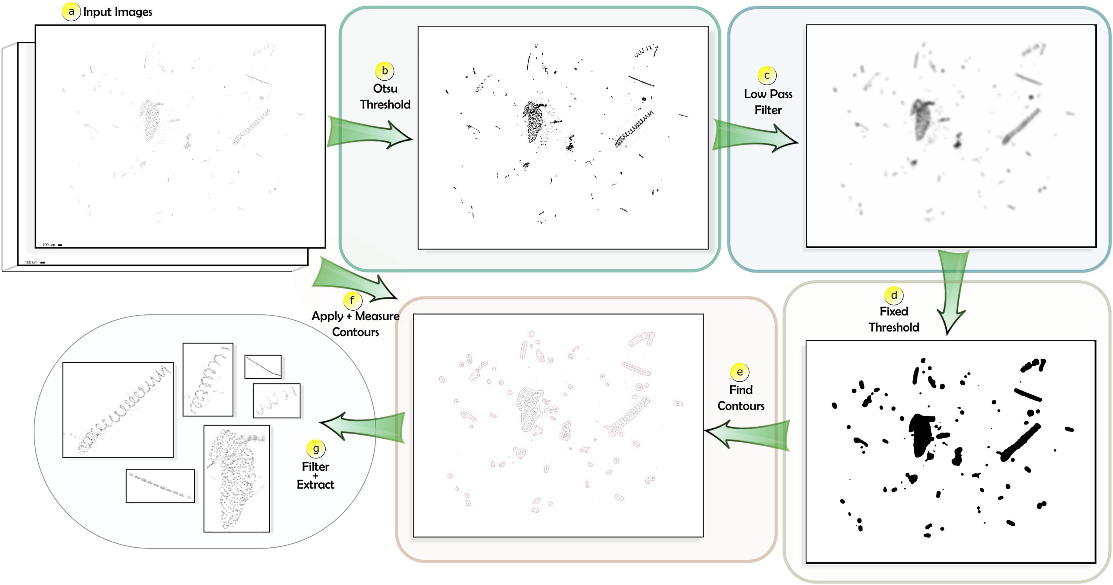
Figure 1. Planktonator segmentation and particle extraction workflow. (a) Input reconstructed images from HoloBatch, (b) Otsu threshold to find the most prominent pixels, (c) low pass filtering to connect neighboring pixels, (d) fixed threshold and flood fill to define particle regions, (e) contour calculation, (f) application of contours and particle measurement, (g) particle filtering and extraction.

FIGURE 2

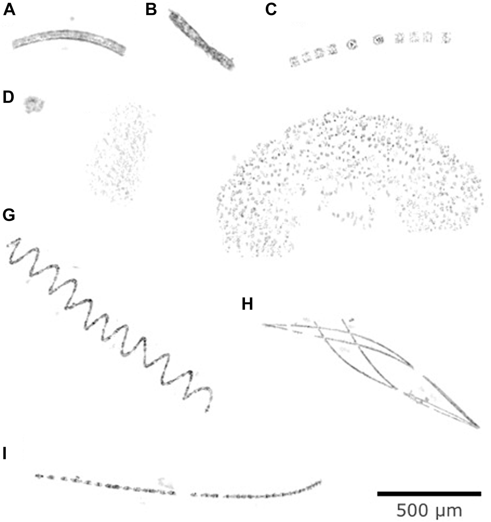
Figure 2. Example vignettes from profile DY086-034 near South Georgia showing most likely (A) Fragilariopsis kerguelensis, (B) fecal pellet, (C) Thalassiosira sp., (D) compact phytodetritus, (E) loose phytodetritus, (F) Chaetoceros socialis, (G) Eucampia antarctica, (H) Thalassiothrix sp., and (I) chain-forming phytoplankton.

We first used Otsu (1979) to convert the monochrome input image into a binary image by minimizing the intra-class variance between the background (water) and foreground (particles), leaving the most prominent pixels with a new pixel intensity of 0. Otsu is also applied as part of the HoloBatch software (Graham and Nimmo Smith, 2010; Davies et al., 2015) and is one of the most commonly referenced thresholding techniques (Sezgin and Sankur, 2004). In the following step a low pass filter with a kernel size of 25 and linearly decreasing spatial weights was applied to produce a blurred non-binary image. This step was used to connect neighboring pixels while maintaining the overall particle shape. The proximity of neighboring (particle) pixels also determines the intensity of pixels in the filtered image; the intensities of isolated and detached pixels (i.e., noise) are reduced while the intensities of tightly compacted pixels are maintained. A threshold was then applied to the filtered image to convert back to a binary image. A lower threshold reduces the detected particle area while a higher threshold increases it. We manually defined this value to be 0.96 (in the range [0,1]) as this produced satisfactory results after visual inspection. The result is an image composed of black regions corresponding to particle areas. As it is possible that a number of these areas contained gaps/holes, we filled holes using a flood fill operation before proceeding to the next stage. Contours were calculated from each particle region using scikit-image³. After obtaining the contour positions we measured each particle to determine their major length. Only particles with a minimum major length of 40 pixels (176 μm) were used for further analyses, as smaller particles typically lacked sufficient detail to be identified. Note that this size threshold was only applied during the segmentation process. The final step was to produce image crops around the detected contours regions. These crops contain data from the original monochrome images generated by HoloBatch and therefore have not been processed by thresholding. The objective of this workflow was to produce vignettes containing a single marine snow particle, and parameters were defined carefully through visual inspection. Nonetheless, without ground truth data, we were unable to verify the outputs objectively and some vignettes may still contain multiple particles.

Thresholding

For size measurements, vignettes were analyzed using Python and scikit-image (see text footnote 3). Vignettes were 8-bit monochrome PNG files with gray values from 0 (black) to 255 (white). The particle in each vignette was identified using a range of static threshold values and 11 different algorithms (seven threshold and four edge detection algorithms). All algorithms used here are provided in the scikit-image filters and features modules. All vignettes (n = 6400) and their metadata including size measurements are provided in the Supplementary Material. Examples of the code can be found in the Supplementary Material and at github.com/brett-hosking/supplementary.

The application of a gray-value threshold is straightforward. A gray value between 0 (black) and 255 (white) is chosen, any pixel below the threshold is considered particle, and any pixel at or above the threshold is considered background. The result is a true-false (binary) image separating the particle and background (also referred to as a “mask”). Particle measurements can then be performed on the binary mask. We tested a range of static thresholds, i.e., we applied the same threshold value to all vignettes. Static thresholds ranged from 10 to 250 in 10-unit increments. In addition, we applied seven histogram-based thresholding algorithms: Otsu, Isodata, Li, Mean, Minimum, Triangle and Yen. These algorithms find a unique threshold value for each vignette based on the image properties (the gray-value histogram). A description and illustration for each of these algorithms is provided in Table 1.

TABLE 1

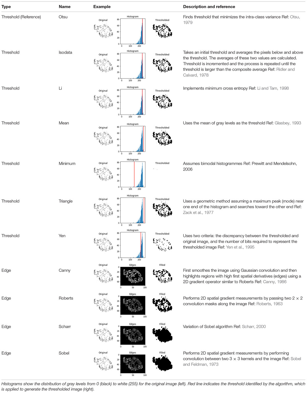
Table 1. Threshold algorithms.

Edge detection algorithms effectively analyze each pixel and its neighbors to detect changes in pixel intensity. A gradient mask is produced that depicts strong gradients as lighter pixels. Depending on the algorithm, the gradient mask is thresholded to retain only the strongest gradients (“edges”). Pixels corresponding to an edge are assigned a “true” value, whereas pixels that are similar to their neighbors are assigned the value “false.” The resulting binary image hence traces the edges of the particle. Using a flood fill operation, all pixels within the detected edges are filled, producing the final binary mask. We applied four common edge detection algorithms: Canny, Sobel, Scharr, and Roberts. A description and illustration for each of these algorithms is provided in Table 1.

We used Otsu as the reference threshold algorithm as it is, as described above, used in the HoloBatch software (Graham and Nimmo Smith, 2010; Davies et al., 2015) and our segmentation routine. Moreover, Otsu is one of the most commonly applied thresholding techniques (Sezgin and Sankur, 2004), and it generally produced (subjectively) reasonable results.

Particle Size and Shape

Once the algorithms were applied to the vignette, we calculated the particle’s size based on the pixel count for the following parameters: area, equivalent spherical diameter (ESD), convex area and Feret length (details in Table 2). The shape of the particle was explored in terms of roundness, i.e., how similar the overall particle shape is to a circle, and solidity, i.e., how densely packed the particle is (Table 2). Both parameters range from 0 to 1, with a value close to 1 suggesting the particle is, respectively, nearly circular or solid. Please note that roundness was calculated using the area of the convex hull rather than the particle area. We chose this metric because many of the large particles were very loosely packed aggregates or colonies. For these cases, the traditional roundness metric (ratio of particle area to Feret length) would suggest that such particles are elongated even though, in reality, they were often round.

TABLE 2

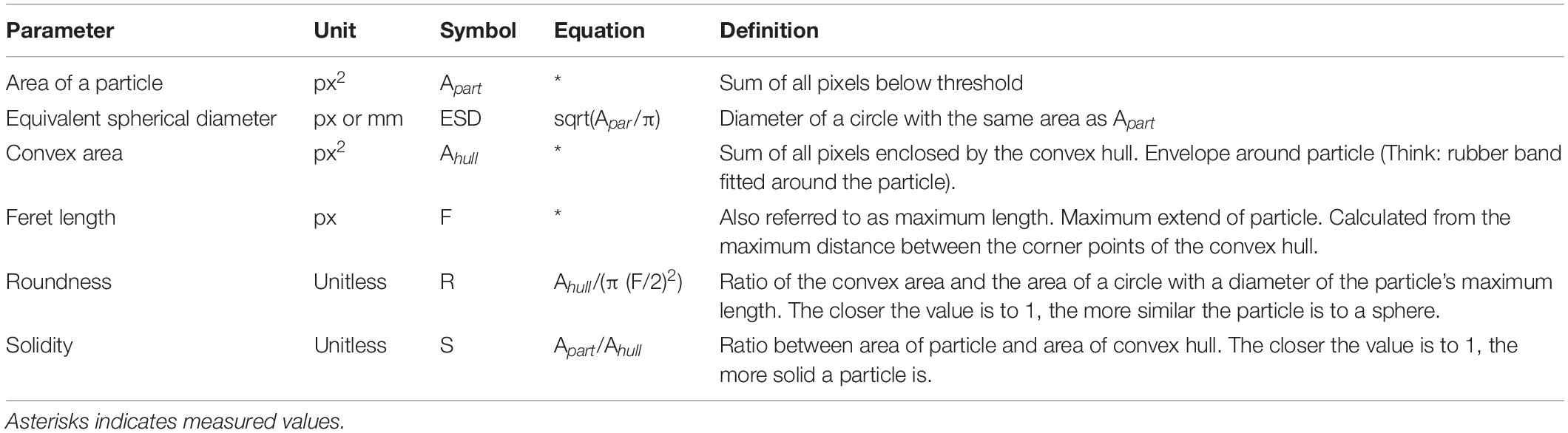
Table 2. Particle size parameters.

POC Content, Sinking Velocities, and Fluxes

POC contents of an individual particle (in μg C) was calculated from the particles volume (V_hull in mm³) using a modification of the equation by Alldredge (1998):

$$\text{POC}=0.99\times V_{hull}{}^{0.52}\times S{}^{3/2}(1)$$

where V_hull is calculated from the hull area [A_hull in mm; V_hull = 4/3 π (A_hull/π)^3/2] and S is the solidity of the particle (Table 2). Hull area was chosen as metric for particle size as it is closer to the area metric used by Alldredge (1998). The original equation by Alldredge (1998) overestimated POC concentrations compared to POC concentrations measured using in situ pumps (53 μm mesh; data not shown), likely because many of the particles that we imaged were very loosely packed. We used the solidity metric (scaled to volume) to account for this discrepancy (i.e., we allowed particles to be porous), which produced an acceptable match between calculated and measured POC concentrations.

Fluxes were calculated by multiplying the POC content of a particle by its estimated sinking velocity. Sinking velocities (v in m d^–1) were assumed to be a function of the particle’s size (ESD_hull in mm) following power law and solidity (S):

$$v={75}^{*}ES{D}_{hull}{}^{0.24}\times S{}^{3/}{}^2(2)$$

The regression was based on in situ data collected during the COMICS cruises. Briefly, an underwater camera was fitted onto a neutrally buoyant sediment trap and programmed to take a fast sequence of images (deployment depth 500 m). Individual sinking particles (n = 244) were tracked through the images and a downward sinking velocity calculated. Most sinking particles were <1 mm in diameter (median 0.20 ± 0.26 mm ESD) similar to our observations (median 0.33 ± 0.47 mm hull-based ESD detected by Otsu). The regression fit was not strong (p < 0.01, R² = 0.08, n = 244) but generally matched previous observations (Table 3). Particles at 500 m were more solid than particles observed in the upper 250 m of the water column, which likely reflected differences in excess density with less solid particles being less dense. We therefore applied the same solidity-based scaling as in Eq. (1). Calculated sinking velocities ranged from 0.2 to 46 m d^–1 with a median of 8 ± 8 m d^–1, which seems plausible for loosely packed particles of a median size of 0.33 mm in hull-based ESD. Please note that the absolute POC concentrations and fluxes presented here are used primarily for illustration purposes to highlight the effect of different thresholds and threshold algorithms on final estimates.

TABLE 3

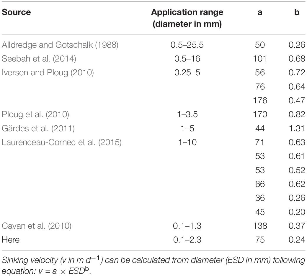
Table 3. Size-to-sinking velocity conversion parameters in the literature.

To compare particle profiles, mean ESD, POC concentrations, and POC fluxes were binned in 1-m bins. Variability was often high between adjacent bins making it difficult to compare the different algorithms. We therefore smoothed depth profiles by calculating a running mean and standard deviation (n = 11) for each depth. Hence, flux at 20 m is the mean of fluxes between 15 and 25 m. The flux attenuation rate (“b parameter”) was calculated by fitting a power-law to the flux profile below 50 m (Martin et al., 1987).

Results

Particle Profiles

The LISST-Holo imaged a wide range of particle types (Figure 2). The number of detected particles and particle concentrations varied markedly between the different deployments (Table 4), reflecting ecological differences between the profiles. Particle abundance was higher near South Georgia (0.5–3.3 particles mL^–1 throughout the sampled water column) compared to the Benguela (<0.1–0.3 particles mL^–1) (Table 4). The highest number of particles was imaged near South Georgia on the 16 Nov 2017 (profile DY086-034) with a total of 2707 vignettes (2.6 particles mL^–1). This high abundance allows us to explore changes in particle characteristics with depth. In contrast, in the profiles in the Benguela, we imaged only a total of 16, 23, and 149 particles, which precludes a meaningful exploration of vertically resolved fluxes.

TABLE 4

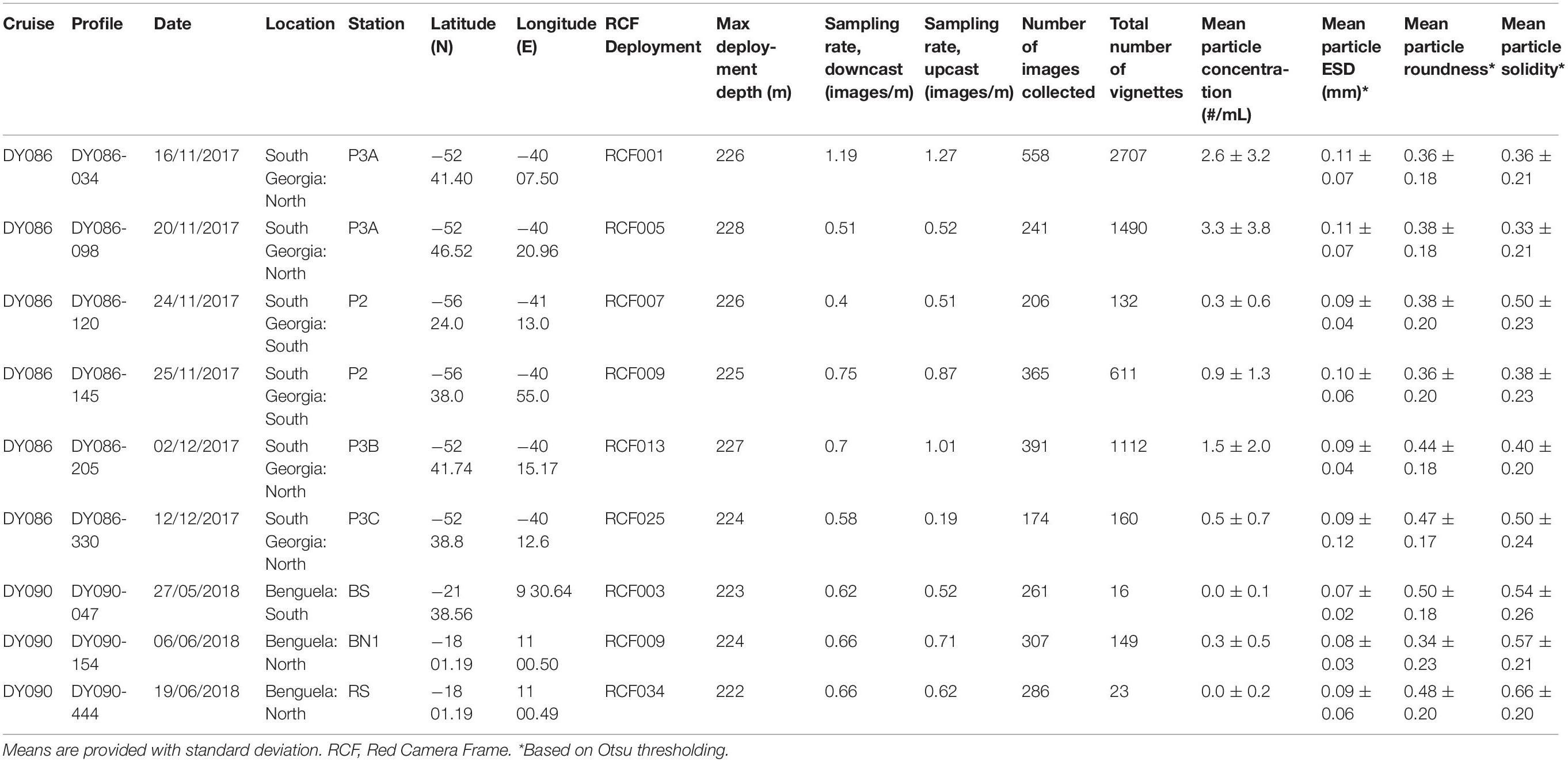
Table 4. Deployment details and simple particle profile statistics.

All particle profiles showed similar depth trends with higher particle concentrations in the upper 100 m and typically <2 particles per mL deeper in the water column (illustrated for profile DY086-034 in Figure 3A). At the northern South Georgia stations, mean particle size (ESD) decreased with increasing depth while roundness and solidity increased (Figures 3B–D). These trends are also apparent at the Southern South Georgia and Benguela stations, though they are less clear owing to the low number of observed particles (data not shown).

FIGURE 3

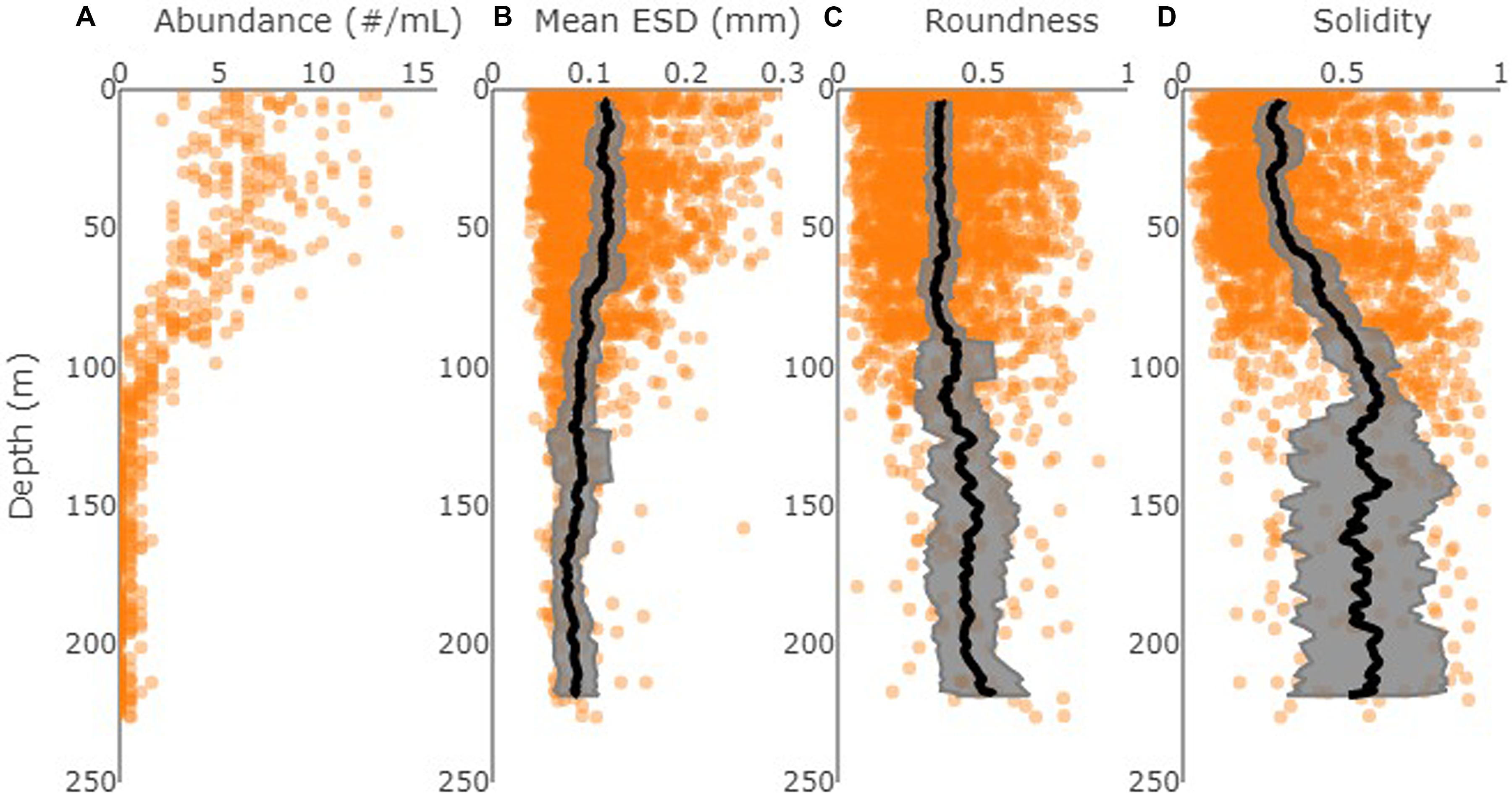
Figure 3. Depth profiles of particle statistics from profile DY086-034 near South Georgia based on Otsu, showing (A) number of particles (per mL calculated for each image), (B) particle ESD (in mm), (C) roundness, and (D) solidity. Black lines show running mean (n = 11) for 1-m binned data. Gray envelopes show the corresponding standard deviation.

Static Threshold

By applying a range of thresholds (10–250) and comparing ESD to that calculated using a threshold of 250, we can clearly see how important the threshold is for the final particle size and flux estimates. First of all, low static thresholds failed to “find” particles in many of the vignettes, i.e., there were no pixels below the threshold gray value and the size was returned as “0” (Figure 4A). Even the static threshold value of 220 returned one empty vignette (out of 6400 vignettes). Estimated ESD increased rapidly between threshold values 160 and 240 at a rate of 1 percentage-point per unit (relative to the ESD at calculated for threshold value 250). In other words, choosing 200 rather than 190 as threshold value resulted in a 10 percent increase in the ESD estimate (from 45 to 55% 250-threshold-equivalent ESD). Accordingly, estimates for sinking velocities, particle POC content and particle-specific POC flux followed the trend in ESD, with a rapid increase in relative values as the threshold value increases (Figure 4B). The additive effect of size on flux estimates resulted in a rapid increase in flux estimates with increasing static threshold (Figure 4C).

FIGURE 4

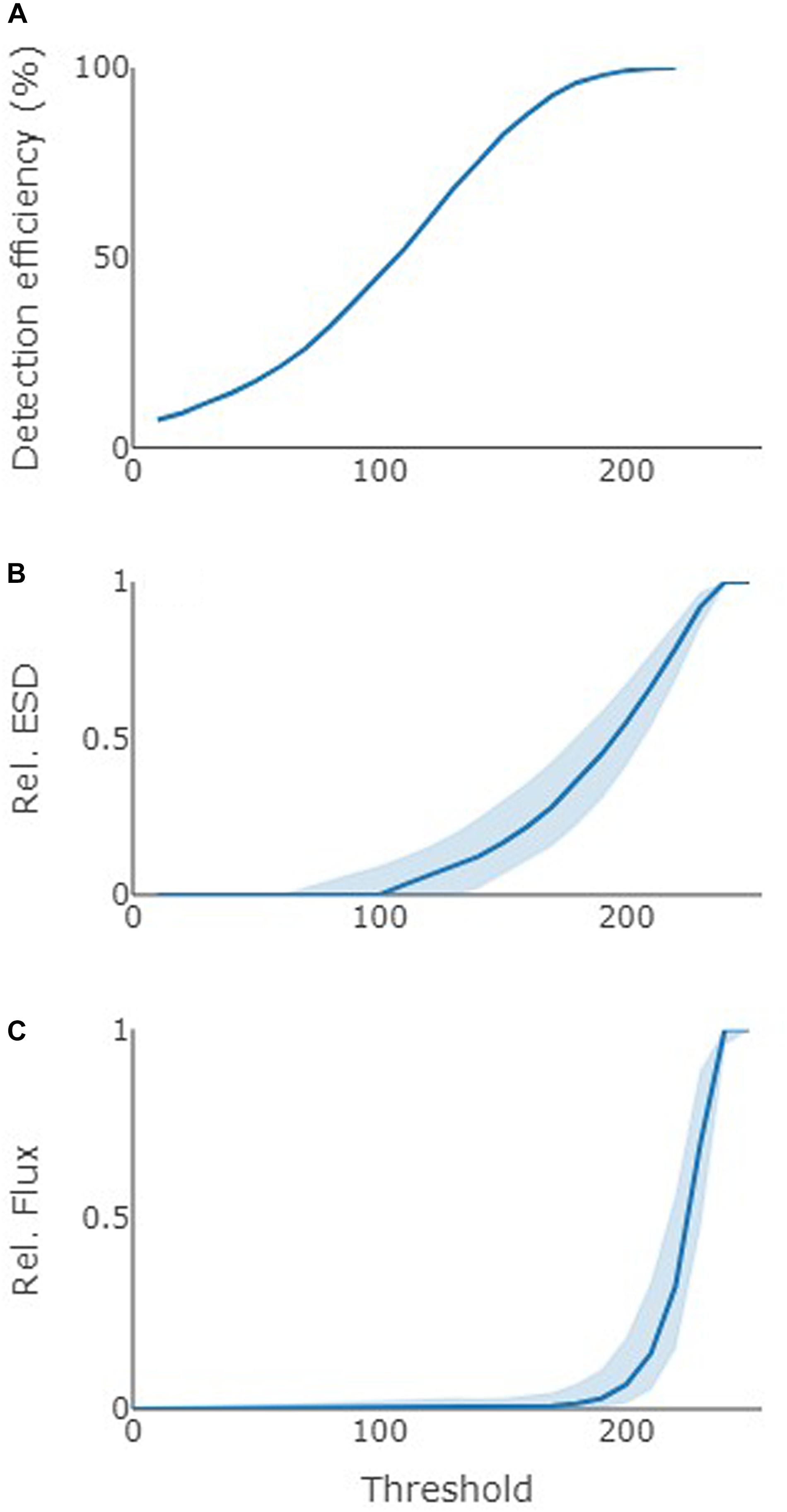
Figure 4. Effect of changing static threshold on (A) detection efficiency (% of total particles), (B) particle ESD (px), and (C) particle-specific POC flux (mg C m^–2 d^–1). All values were normalized to those calculated with a threshold of 250. Lines show the median. Blue polygon encompasses upper and lower quartile. Based on all imaged particles (n = 6400).

Algorithm Choice

The different threshold algorithms calculated a range of thresholds, with median estimates ranging from 126 (Minimum) to 254 (Triangle) (Figure 5). Otsu estimates were generally in the intermediate range (median 227) and similar to estimates by IsoData and Li (median 227 and 224; Figure 5). The algorithm Minimum calculated lower thresholds (median 126), whilst Mean, Triangle and Yen tended to calculate higher threshold values (median 250, 254, and 233, respectively, Figure 5).

FIGURE 5

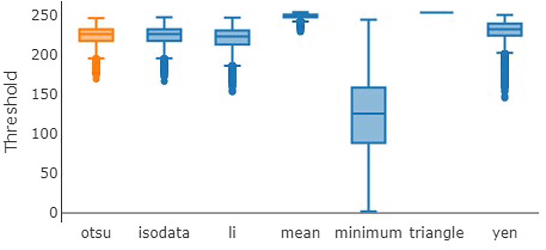
Figure 5. Threshold values calculated for all vignettes using different algorithms. Colors show threshold algorithm type as orange (reference algorithm) and blue (binary). Values are expressed as boxplots, showing median (horizontal line), first and third quartile range (box), minimum and maximum values (error bars), and outliers (dots). Based on all imaged particles (n = 6400).

The choice of threshold algorithm had a marked influence on the estimates of particle size, carbon content, sinking velocity (data not shown) and flux for each vignette (Figure 6). Binary algorithms that detected low thresholds (Li and Minimum) estimated lower particle parameter values, while the algorithms that detected higher thresholds (Mean, Triangle, and Yen) estimated higher particle parameter values. Owing to the conversion steps, these differences magnified from ESD to POC content to POC flux for each particle (Figure 6). For example, the respective estimates using Mean (relative to Otsu) were (median) 112, 129, and 156% for ESD, POC content, and POC flux.

FIGURE 6

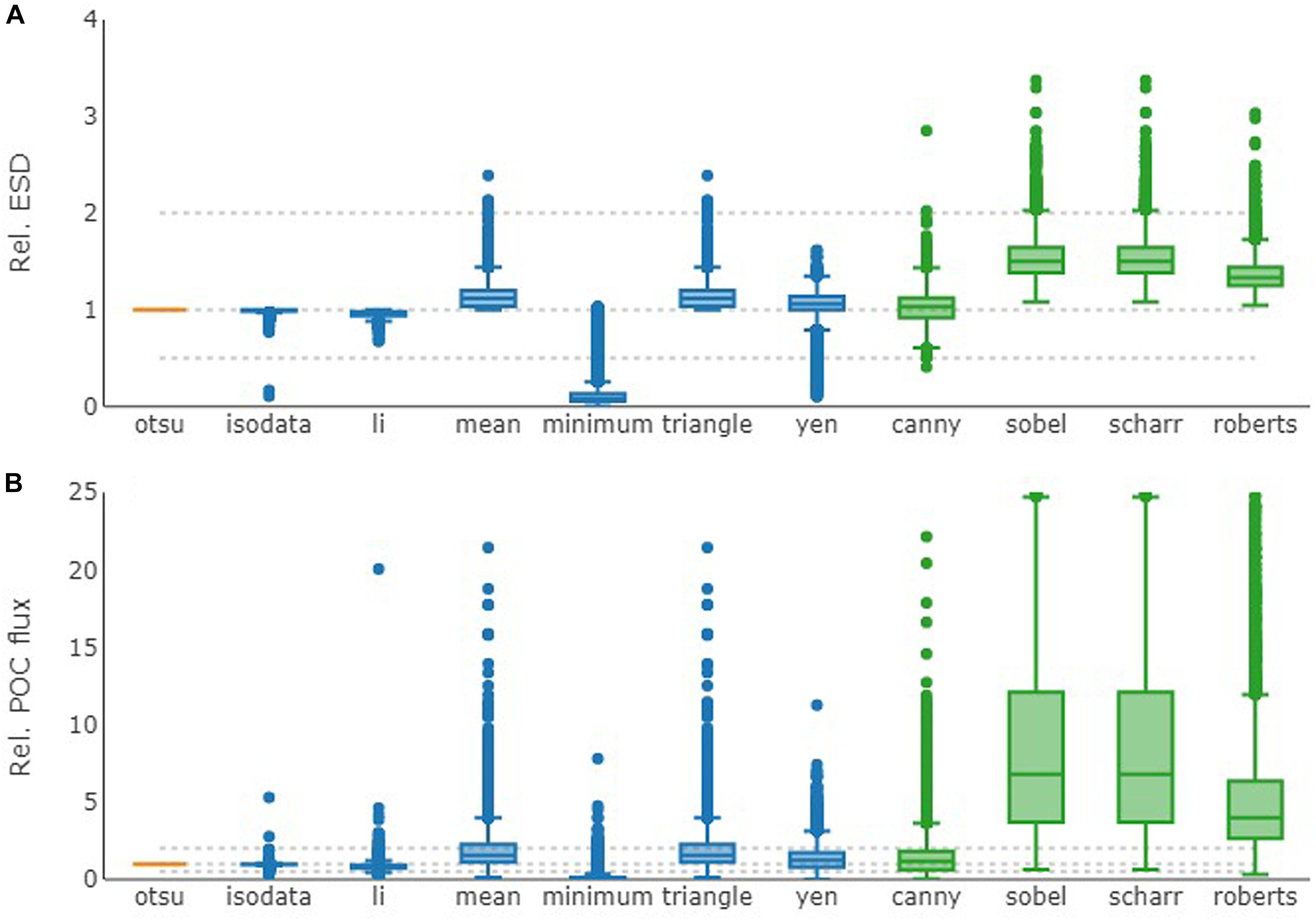
Figure 6. Comparison of different threshold algorithms relative to Otsu. (A) Particle size (ESD in mm). (B) Average POC flux per particle (mg C m^–2 d^–1). Values are expressed as boxplots (see legend for Figure 5). Gray dashed lines indicate 0.5, 1, and 2 times Otsu value. Note the different y-axis scales. Colors show threshold algorithm type as orange (reference algorithm Otsu), blue (binary), and green (edge detection). Based on all imaged particles (n = 6400).

The four edge-detection algorithms all calculated larger particles with, accordingly, higher carbon content, sinking velocities and fluxes. In the order of ascending estimated particle size, the algorithms were Canny, Roberts, and, jointly, Sobel and Scharr (median ESD relative to Otsu 103, 133, 150, and 150%, respectively). The POC flux for an individual vignette estimated by Sobel and Scharr were up to 670 times that by Otsu. Even though this was an extreme, median flux estimates were still 6.8 times that by Otsu.

Vertical flux profiles from the first station (DY086-034 at the northern South Georgia site) followed the expected decrease in flux from the surface to depth for all algorithms, though the overall flux magnitude differed greatly (Figure 7). For example, the flux at 100 m according to Otsu was 278 mg C m^–2 d^–1 (Figure 7). The algorithms Minimum, Li and Isodata estimated the flux to be 16, 74, and 93% of this value, respectively. On the other hand, the algorithms Yen, Mean, Triangle, Canny, Roberts, Sobel, and Scharr estimated the flux to be much higher at 118, 153, 153, 173, 245, 318, and 318%, respectively. Hence, when using the Sobel or Scharr algorithms, particle flux at 100 m would have been estimated 886 mg C m^–2 d^–1; a carbon supply to the deep ocean of ∼600 mg C m^–2 d^–1 more (Figure 7).

FIGURE 7

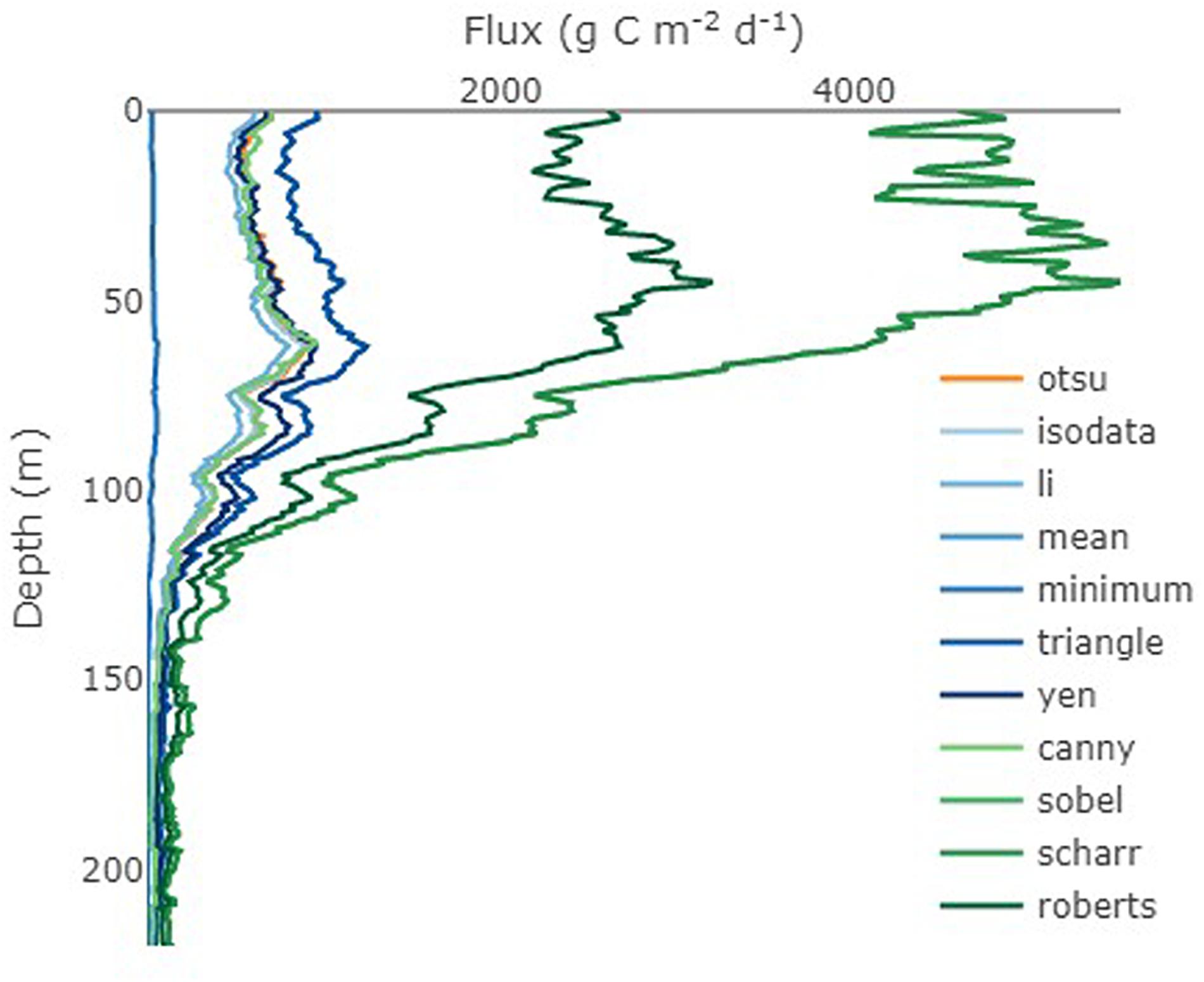
Figure 7. Flux profiles from deployment DY086-34 near South Georgia according to the different threshold algorithms. Fluxes were calculated for all particles as described in the methods and summed for each vignette. Flux profiles were binned at 1-m resolution and a running mean (n = 11) calculated.

In addition, the different algorithms gave slightly different vertical shapes. Fitting a power-law to the flux profile below 50 m (Martin et al., 1987) suggests that the flux attenuation rate (“b parameter”) at the first station (DY086-034 at the northern South Georgia site) varied from 2.29 to 2.96 depending on the flux algorithm (Minimum and Sobel/Scharr, respectively).

We observed a large effect of algorithm choice on median particle size (ESD), POC concentrations, flux estimates, and flux attenuation rate (“b parameter”) at all sites (Table 5).

TABLE 5

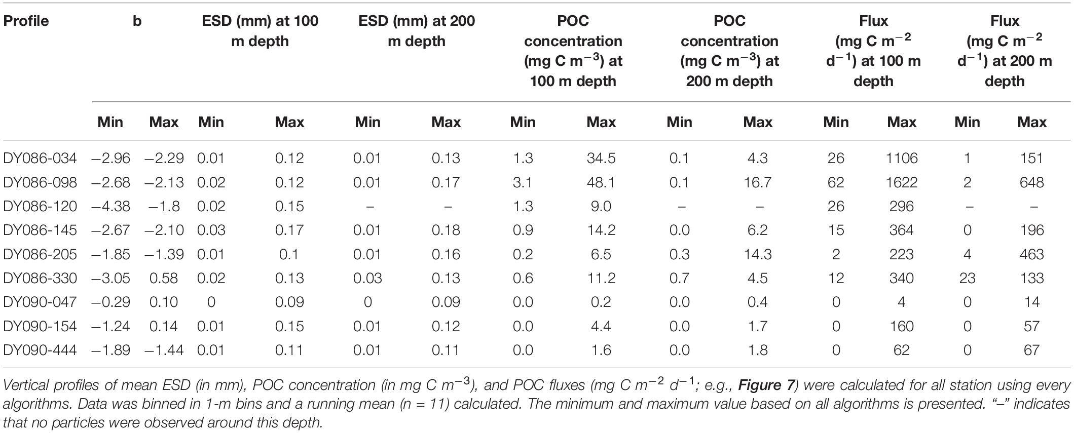
Table 5. Variability of particle characteristics at all stations based on vertical profiles.

Solidity and Roundness

Observed particles ranged in solidity from very loosely aggregated (S < 0.1) to solid (S > 0.9). The median solidity of the particle population was strongly dependent on the threshold algorithm (Figure 8). The highest median solidity was estimated by the binary algorithm Minimum, with a median solidity of 0.83. The edge detection algorithms Roberts, Sharr and Sobel diagnosed high solidities with a median of 0.48–0.56. Canny and the other binary algorithms calculated median solidity values between 0.30 and 0.36. The static thresholds below a gray value of 60 also diagnosed very solid particles, but owing to their poor performance (>75% of analyzed vignettes were “empty”), these are not further discussed.

FIGURE 8

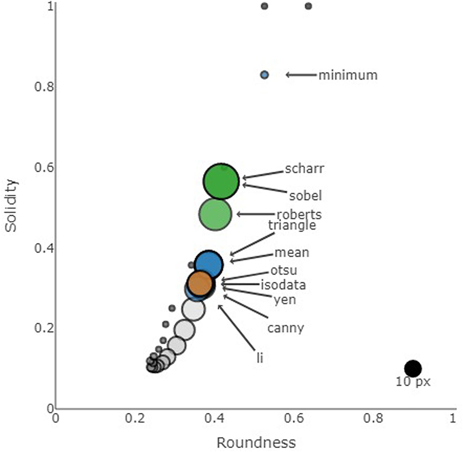
Figure 8. Median roundness and solidity for all threshold algorithms. The symbol size shows the median particle size for each algorithm (reference point of 10 px in diameter shown in black in bottom right corner). Blue symbols: binary algorithms, orange symbol: Otsu, green symbols: edge detection algorithms, gray symbols: static threshold with symbol color representing the threshold. Based on all imaged particles (n = 6400).

There was no consistent relationship between particle size and solidity, though the density plots suggest two loose clusters (Figure 9). The most prominent cluster comprised of particles with a diameter of around 20 px (∼88 μm) and a relatively low solidity (S∼0.25). There was a second cluster of particles with a similar diameter but much rounder shape (R > 0.75). For all algorithms, particles with an ESD of >30 px (∼132 μm) appeared to become less solid as they got larger.

FIGURE 9

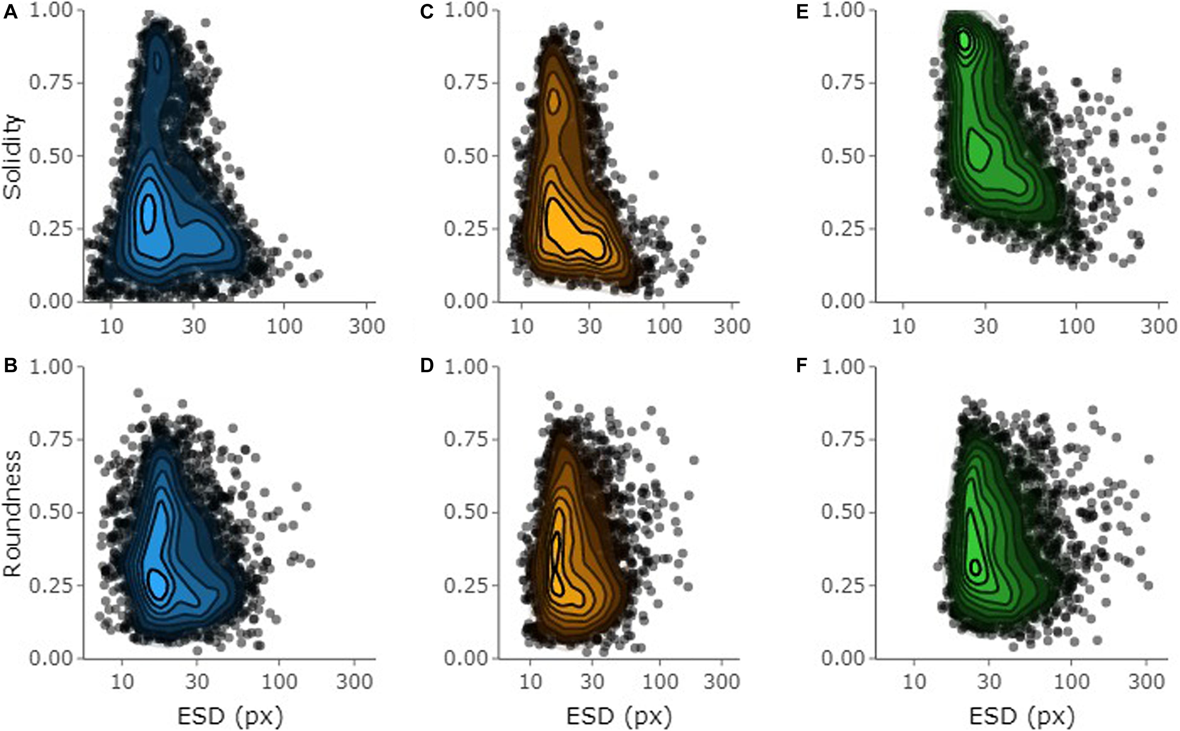
Figure 9. Heat map of (A–C) solidity and (D–F) roundness of particles as a function of size (ESD in pixels) for profile DY086-034 near South Georgia. The closer the values are to 1, the more solid and circle-like the particles are. Note the logarithmic scale for the x-axis. Values based on (A,B) Yen (blue), (C,D) Otsu (orange), and (E,F) Sobel (green) thresholding. Lighter colors indicate higher density of data points. Pixel size: 4.4 μm.

We next investigated the roundness of particles according to the different algorithms. The population median was similar for all binary (except Minimum) and edge detection algorithms, ranging from 0.36 to 0.42 (Figure 8). The Minimum algorithm estimated particles to be rounder (median: 0.53), while the static thresholds above 60 estimated particles to be more elongated (median: 0.24–0.39). As static thresholds increased from 140 onward, the median roundness increased consistently (Figure 8). There was no clear trend between particle ESD and roundness (Figure 9). Please keep in mind, however, that the trends observed here might be a result of the optical device and its resolution rather than an overall ecological phenomenon.

Discussion

Particle Size

Our error estimates are likely conservative owing to the LISST-Holo methodology: As the LISST-Holo uses diffraction pattern to reconstruct particles rather than conventional photography, the reconstructed particle images have relatively clear edges (Graham and Nimmo Smith, 2010). Conventional cameras often struggle with lighting artifacts such as halo-like boundaries around the particle (e.g., Farhadifard et al., 2017), refraction and semi-transparent edges. It is hence surprising and worrying that, even with well-defined particle edges in the LISST-Holo vignettes, the effect of the threshold algorithm choice on final size and flux estimates are significant.

Particle size estimates appear to be highly sensitive to even small changes in threshold values. One advantage of threshold algorithms is that they are easy to understand and sensitivity analyses are uncomplicated. For example, to explore the effect on particle size, a defined number can be added or subtracted from the estimated threshold value before recalculating size. Edge detection algorithms are more complex and the results not as straightforward to evaluate particularly for aggregates with complex textures. These algorithms generally produced particle size estimates that exceeded those of the threshold algorithms. A possible reason for this phenomenon is the nature of the processing used to produce a binary mask from the detected particle outline, and the fact that edges in the binary image were not always clearly defined (i.e., pixels at edge boundaries were often noisy). This noise resulted in detected edges that appeared extruded, thus the binary mask covered a larger area. In addition, the Scharr and Sobel detectors also treat loose and closely connected aggregates as a single continuous particle, producing a mask that covers a large area (see example in Table 1). The Canny edge detector often produced edges that were not enclosed and therefore, when applying the flood fill operation, the masks only represented a portion of the visually determined particle shape. This partial filling explains why this algorithm produced smaller particle size estimates compared to the other edge detectors, though, perhaps surprisingly, the average particle sizes calculated by Canny were the same as those calculated by Otsu.

The effect of such nuances on final flux estimates is potentially huge, with our estimates by different algorithms varying by an order of magnitude. Our data highlights the importance of thorough calibration of the particle sizing routines and detailed method descriptions.

Researchers need to be very careful and considerate when choosing the particle detection and sizing algorithms. Simple visual inspection is a potential first step and may help to select a suitable algorithm for the particle type (e.g., compare raw and binary images in Table 1). However, algorithm choice by eye alone is not sufficient: both Li and Triangle appear to trace the example particle in Table 1 well, but their estimated area differed by ∼20% (1146 and 1386 px², respectively). Rather, the sizing algorithm needs to be calibrated using external reference material. The developers of the Underwater Vision Profiler (UVP) calibrate each newly built UVP by deploying the new UVP alongside a “reference” UVP, which had been calibrated using natural marine snow and zooplankton (Picheral et al., 2010). While this is a good instrument-specific approach, it is not a feasible strategy for comparison between different instrument types and when comparing in situ and ex situ devices. Sosik et al. (pers. comm.) used a range of beads to fine-tune an edge detection algorithm for the FlowCytobot. When applied to phytoplankton cells of a known size-range, the new algorithm calculated much more realistic size estimate (unpublished data).

Particle Shape

The trend of particles to become less solid as size increases matches visual inspection of the vignettes. Many of the small vignettes contained relatively well-contained shapes, whereas many of the large vignettes depicted long diatom chains, such as Eucampia spp. (Figure 2G), and loose aggregates. This trend was the same for all threshold levels, suggesting – at face value – that the overall particle shapes were preserved (Figure 9). However, the median population solidity was different for the different thresholds (Figure 8), likely because an increase in threshold leads to the inclusion of more pixels, which filled in the “holes.”

The effect of including lighter pixels on particle size and shape is also indicated in the roundness of particles (Figure 8). Those algorithms with a higher median threshold estimated particles to be both larger and rounder. An increase in roundness was likely a result of, as for solidity, higher thresholds including more pixels, such as “peripheral” pixels.

The complex relationship between size, solidity and roundness highlights problems when reducing images to simple particle metrics such as ESD. Figure 2F, for example, shows a colony (likely the diatom Chaetoceros socialis) that forms large structures made of shorter chains of individual cells. As a consequence, this particle is very loosely packed with a large fraction of the particle within the convex hull being above the threshold (S = 0.20). The traditional roundness metric (area/F) suggests that this particle is very elongated (R_trad = 0.10), equivalent to an ellipse with a width of 30 px. However, the effective width of the particle (width of ellipse with equivalent hull area and maximum length) is 154 px. Our adapted roundness metric, which uses the hull instead, suggests that the particle is reasonably round (R = 0.52), which matches the particle image much better. An inappropriate choice of particle shape descriptor that does not take into account the particle’s solidity and/or an inappropriate choice of threshold settings will result in a wrong description of the particle population. Such distinctions are important for the interpretation and modeling of how particles behave, e.g., in terms of sinking velocity and aggregation/disaggregation.

Conclusion

We here show that the choice of threshold algorithm is critical in particle sizing and, consequently, POC concentration and flux estimates. The final estimates can vary by >20% when selecting different algorithms for analysing a single dataset. This uncertainty is exacerbated when different methods are mixed, such like the cases when datasets from different studies or even devices are merged.

The knock-on effects of “blindly” mixing data sets are likely most severe when the estimated particle sizes are run through a series of conversions, as was done here. (1) First, we imaged particles and estimated ESD using one method and threshold setting. (2) We then used a conversion from ESD to POC contents that was based on a different camera system with an unknown threshold setting and calibration. (3) We estimated the sinking velocity based on data from a third camera system, again without clear knowledge of the image analysis routine and calibration. (4) Finally, we multiplied POC contents and sinking velocities to arrive at POC fluxes. Each step introduces uncertainties leading, potentially, to large errors in the final estimate of POC contents and fluxes. For example, before accounting for solidity when calculating particle POC content (Eq. 1), calculated POC concentrations based on particle images were up to an order of magnitude higher than measured concentrations.

The interpretation of particle shapes (e.g., solidity and roundness) is also affected. Image analysis routines that set a high threshold, and thus include more pixels, will not only estimate particles to be larger than those using a low threshold but also to have a different shape and density. Uncertainty in particle shapes has implications for data interpretation (e.g., density, sinking behavior) and particle modeling (e.g., aggregation/disaggregation; Burd and Jackson, 2009).

We conclude that it is important to make an informed decision on the particle detection algorithm when analysing particle images, and we therefore make the following recommendations:

1. The thresholding decision should be justified and clearly stated in the method section for each study.

2. The threshold choice should be based on calibrations with beads or natural aggregates of known size.

3. The equations used to describe particle size and shape should be clearly stated.

4. To allow merging datasets from different devices, all devices should be calibrated using the same calibration standard.

Currently, there are no calibration standards for particle sizing and no specifications on how to report thresholding. We therefore urge a collective effort to develop calibration routines and specifications to accurately describe particle size. Optical particle measurements are rapidly emerging as a major tool for understanding biogeochemical cycles and food webs in the ocean (Lombard et al., 2019; Giering et al., 2020). To fully leverage these exciting technological advances and the insights they provide, the research community needs a framework that encourages increased transparency in image analysis routines (including threshold choices) and allows merging data from the plethora of optical devices that are now used to explore the ocean.

Data Availability Statement

All vignettes (n = 6400) and their metadata including size measurements are provided in the Supplementary Material. Examples of the code used to take particle size measurements can be found in the Supplementary Material and at github.com/brett-hosking/supplementary.

Author Contributions

SG designed the study and wrote the manuscript with support from all authors. BH wrote the image analysis codes. NB contributed to the method development and interpretation of the results. MI contributed to the data. All authors contributed to the article and approved the submitted version.

Funding

This work was funded by the UKRI through the COMICS project (Controls over Ocean Mesopelagic Interior Carbon Storage; NE/M020835/1) and the National Capability funding. Contributions by NB were funded by a European Research Council Consolidator grant (GOCART, agreement no. 724416). This publication resulted in part from support from the U.S. National Science Foundation (Grant OCE-1840868) to the Scientific Committee on Oceanic Research (SCOR) and from funds contributed by National SCOR Committees.

Conflict of Interest

The authors declare that the research was conducted in the absence of any commercial or financial relationships that could be construed as a potential conflict of interest.

Acknowledgments

We thank Isabell Klawonn, Filipa Carvalho, Richard Lampitt, and Kevin Saw for the deployment of the Red Camera Frame. We also thank Calum Preece, Kostas Kiriakoulakis, and George Wolff for providing data on water-column POC concentrations. Our thanks extend to the captain and crew of the research cruises DY086 and DY090. We thank Brian Bett and Henry Ruhl for providing valuable recommendations about the LISST-Holo setup and deployments. We further thank Adrian Burd and the reviewers for feedback on the manuscript. Last, we thank the Scientific Committee on Oceanic Research (SCOR) and all members of the Working Group 150 (TOMCAT: Translation of Optical Measurements into particle Content, Aggregation & Transfer) for stimulating this work.

Supplementary Material

The Supplementary Material for this article can be found online at: https://www.frontiersin.org/articles/10.3389/fmars.2020.00564/full#supplementary-material

Footnotes

1. ^ sequoiasci.com/product/lisst-holo
2. ^ pypi.org/project/planktonator/ and github.com/brett-hosking/planktonator
3. ^ scikit-image.org

References

Alldredge, A. (1998). The carbon, nitrogen and mass content of marine snow as a function of aggregate size. Deep Sea Res. Part I Oceanogr. Res. Pap. 45, 529–541. doi: 10.1016/S0967-0637(97)00048-44

CrossRef Full Text | Google Scholar

Alldredge, A. L., and Gotschalk, C. (1988). In situ settling behavior of marine snow. Limnol. Oceanogr. 33, 339–351. doi: 10.4319/lo.1988.33.3.0339

CrossRef Full Text | Google Scholar

Basu, M. (2002). Gaussian-based edge-detection methods-a survey. IEEE Trans. Syst. Man Cybern. Part C 32, 252–260. doi: 10.1109/TSMCC.2002.804448

CrossRef Full Text | Google Scholar

Burd, A. B., and Jackson, G. A. (2009). Particle aggregation. Ann. Rev. Mar. Sci. 1, 65–90. doi: 10.1146/annurev.marine.010908.163904

PubMed Abstract | CrossRef Full Text | Google Scholar

Canny, J. (1986). A computational approach to edge detection. IEEE Trans. Pattern Anal. Mach. Intell. 8, 679–698. doi: 10.1109/TPAMI.1986.4767851

CrossRef Full Text | Google Scholar

Cavan, E. L., Giering, S. L. C., Wolff, G. A., Trimmer, M., and Sanders, R. (2018). Alternative particle formation pathways in the eastern tropical north pacific’s biological carbon pump. J. Geophys. Res. Biogeosci. 123, 2198–2211. doi: 10.1029/2018JG004392

CrossRef Full Text | Google Scholar

Davies, E. J., Buscombe, D., Graham, G. W., and Nimmo-Smith, W. A. M. (2015). Evaluating unsupervised methods to size and classify suspended particles using digital in-line holography. J. Atmos. Ocean. Technol. 32, 1241–1256. doi: 10.1175/JTECH-D-14-00157.1

CrossRef Full Text | Google Scholar

Durkin, C. A., Estapa, M. L., and Buesseler, K. O. (2015). Observations of carbon export by small sinking particles in the upper mesopelagic. Mar. Chem. 175, 72–81. doi: 10.1016/j.marchem.2015.02.011

CrossRef Full Text | Google Scholar

Farhadifard, F., Radolko, M., and Freiherr von Lukas, U. (2017). “Single image marine snow removal based on a supervised median filtering scheme,” in Proceedings of the 12th International Joint Conference on Computer Vision, Imaging and Computer Graphics Theory and Applications, (Setúbal: SCITEPRESS - Science and Technology Publications), 280–287.

Google Scholar

Flintrop, C. M., Rogge, A., Miksch, S., Thiele, S., Waite, A. M., and Iversen, M. H. (2018). Embedding and slicing of intact in situ collected marine snow. Limnol. Oceanogr. Methods 16, 339–355. doi: 10.1002/lom3.10251

CrossRef Full Text | Google Scholar

Gärdes, A., Iversen, M. H., Grossart, H.-P., Passow, U., and Ullrich, M. S. (2011). Diatom-associated bacteria are required for aggregation of Thalassiosira weissflogii. ISME J. 5, 436–445. doi: 10.1038/ismej.2010.145

PubMed Abstract | CrossRef Full Text | Google Scholar

Giering, S. L. C., Cavan, E. L., Basedow, S. L., Briggs, N., Burd, A. B., Darroch, L., et al. (2020). Sinking organic particles in the ocean - what can we learn from optical devices? Front. Mar. Sci. 6:834. doi: 10.3389/fmars.2019.00834

CrossRef Full Text | Google Scholar

Giering, S. L. C., Sanders, R., Martin, A. P., Lindemann, C., Möller, K. O., Daniels, C. J., et al. (2016). High export via small particles before the onset of the North Atlantic spring bloom. J. Geophys. Res. Ocean. 121, 6929–6945. doi: 10.1002/2016JC012048

CrossRef Full Text | Google Scholar

Glasbey, C. A. (1993). An analysis of histogram-based thresholding algorithms. CVGIP Graph. Model. Image Process. 55, 532–537. doi: 10.1006/cgip.1993.1040

CrossRef Full Text | Google Scholar

Graham, G. W., and Nimmo Smith, W. A. M. (2010). The application of holography to the analysis of size and settling velocity of suspended cohesive sediments. Limnol. Oceanogr. Methods 8, 1–15. doi: 10.4319/lom.2010.8.1

CrossRef Full Text | Google Scholar

Grossart, H., Kiørboe, T., Tang, K., Allgaier, M., Yam, E., and Ploug, H. (2006). Interactions between marine snow and heterotrophic bacteria: aggregate formation and microbial dynamics. Aquat. Microb. Ecol. 42, 19–26. doi: 10.3354/ame042019

CrossRef Full Text | Google Scholar

Iversen, M. H., Nowald, N., Ploug, H., Jackson, G. A., and Fischer, G. (2010). High resolution profiles of vertical particulate organic matter export off Cape Blanc, Mauritania: degradation processes and ballasting effects. Deep Sea Res. Part I Oceanogr. Res. Pap. 57, 771–784. doi: 10.1016/j.dsr.2010.03.007

CrossRef Full Text | Google Scholar

Iversen, M. H., and Ploug, H. (2010). Ballast minerals and the sinking carbon flux in the ocean: carbon-specific respiration rates and sinking velocity of marine snow aggregates. Biogeosciences 7, 2613–2624. doi: 10.5194/bg-7-2613-2010

CrossRef Full Text | Google Scholar

Laurenceau-Cornec, E., Trull, T., Davies, D., De La Rocha, C., and Blain, S. (2015). Phytoplankton morphology controls on marine snow sinking velocity. Mar. Ecol. Prog. Ser. 520, 35–56. doi: 10.3354/meps11116

CrossRef Full Text | Google Scholar

Li, C. H., and Tam, P. K. S. (1998). An iterative algorithm for minimum cross entropy thresholding. Pattern Recognit. Lett. 19, 771–776. doi: 10.1016/S0167-8655(98)00057-59

CrossRef Full Text | Google Scholar

Lombard, F., Boss, E., Waite, A. M., Vogt, M., Uitz, J., Stemmann, L., et al. (2019). Globally consistent quantitative observations of planktonic ecosystems. Front. Mar. Sci. 6:196. doi: 10.3389/fmars.2019.00196

CrossRef Full Text | Google Scholar

Lyons, M. M., Lau, Y.-T., Carden, W. E., Ward, J. E., Roberts, S. B., Smolowitz, R., et al. (2007). Characteristics of marine aggregates in shallow-water ecosystems: implications for disease ecology. Ecohealth 4, 406–420. doi: 10.1007/s10393-007-0134-130

CrossRef Full Text | Google Scholar

Martin, J. H., Knauer, G. A., Karl, D. M., and Broenkow, W. W. (1987). VERTEX: carbon cycling in the northeast Pacific. Deep Sea Res. Part A Oceanogr. Res. Pap. 34, 267–285. doi: 10.1016/0198-0149(87)90086-90080

CrossRef Full Text | Google Scholar

McDonnell, A. M. P. (2011). Marine Particle Dynamics: Sinking Velocities, Size Distributions, Fluxes, and Microbial Degradation Rates. Cambridge, MA: Massachusetts Institute of Technology.

Google Scholar

McDonnell, A. M. P., and Buesseler, K. O. (2010). Variability in the average sinking velocity of marine particles. Limnol. Oceanogr. 55, 2085–2096. doi: 10.4319/lo.2010.55.5.2085

CrossRef Full Text | Google Scholar

Ohman, M. D., Davis, R. E., Sherman, J. T., Grindley, K. R., Whitmore, B. M., Nickels, C. F., et al. (2019). Zooglider: an autonomous vehicle for optical and acoustic sensing of zooplankton. Limnol. Oceanogr. Methods 17, 69–86. doi: 10.1002/lom3.10301

CrossRef Full Text | Google Scholar

Otsu, N. (1979). A threshold selection method from gray-level histograms. IEEE Trans. Syst. Man. Cybern. 9, 62–66. doi: 10.1109/TSMC.1979.4310076

CrossRef Full Text | Google Scholar

Picheral, M., Guidi, L., Stemmann, L., Karl, D. M., Iddaoud, G., and Gorsky, G. (2010). The Underwater Vision Profiler 5: an advanced instrument for high spatial resolution studies of particle size spectra and zooplankton. Limnol. Oceanogr. Methods 8, 462–473. doi: 10.4319/lom.2010.8.462

CrossRef Full Text | Google Scholar

Ploug, H., Terbrüggen, A., Kaufmann, A., Wolf-Gladrow, D., and Passow, U. (2010). A novel method to measure particle sinking velocity in vitro, and its comparison to three other in vitro methods. Limnol. Oceanogr. Methods 8, 386–393. doi: 10.4319/lom.2010.8.386

CrossRef Full Text | Google Scholar

Prewitt, J. M. S., and Mendelsohn, M. L. (1966). The analysis of cell images^∗. Ann. N. Y. Acad. Sci. 128, 1035–1053. doi: 10.1111/j.1749-6632.1965.tb11715.x

PubMed Abstract | CrossRef Full Text | Google Scholar

Ridler, T., and Calvard, S. (1978). Picture thresholding using an iterative selection method. IEEE Trans. Syst. Man. Cybern. 8, 630–632. doi: 10.1109/TSMC.1978.4310039

CrossRef Full Text | Google Scholar

Roberts, L. (1963). Machine Perception of Three-Dimensional Solids. Lexington, MA: M.I.T. Lincoln Laboratory.

Google Scholar

Sanders, R. J., Henson, S. A., Martin, A. P., Anderson, T. R., Bernardello, R., Enderlein, P., et al. (2016). Controls over ocean mesopelagic interior carbon storage (COMICS): fieldwork, synthesis, and modeling efforts. Front. Mar. Sci. 3:136. doi: 10.3389/fmars.2016.00136

CrossRef Full Text | Google Scholar

Scharr, H. (2000). Optimal Operators in Digital Image Processing. Ph.D. Dissertation, Heidelberg University, Heidelberg.

Google Scholar

Seebah, S., Fairfield, C., Ullrich, M. S., and Passow, U. (2014). Aggregation and sedimentation of Thalassiosira weissflogii (diatom) in a warmer and more acidified future ocean. PLoS One 9:e112379. doi: 10.1371/journal.pone.0112379

PubMed Abstract | CrossRef Full Text | Google Scholar

Sezgin, M., and Sankur, B. (2004). Survey over image thresholding techniques and quantitative performance evaluation. J. Electron. Imaging 13:146. doi: 10.1117/1.1631315

CrossRef Full Text | Google Scholar

Sobel, I., and Feldman, G. (1973). A 3x3 isotropic gradient operator for image processing. Pattern Classif. Scene Anal. 1973, 271–272.

Google Scholar

Sosik, H. M., and Olson, R. J. (2007). Automated taxonomic classification of phytoplankton sampled with imaging-in-flow cytometry. Limnol. Oceanogr. Methods 5, 204–216. doi: 10.4319/lom.2007.5.204

CrossRef Full Text | Google Scholar

Thompson, C. M., Hare, M. P., and Gallager, S. M. (2012). Semi-automated image analysis for the identification of bivalve larvae from a Cape Cod estuary. Limnol. Oceanogr. Methods 10, 538–554. doi: 10.4319/lom.2012.10.538

CrossRef Full Text | Google Scholar

Volk, T., and Hoffert, M. I. (1985). The Carbon Cycle and Atmospheric CO2: Natural Variations Archean to Present. Washington, DC: American Geophysical Union.

Google Scholar

Yen, J.-C., Chang, F.-J., and Chang, S. (1995). A new criterion for automatic multilevel thresholding. IEEE Trans. Image Process. 4, 370–378. doi: 10.1109/83.366472

CrossRef Full Text | Google Scholar

Yu, X., Wei, Y., Zhu, M., and Zhou, Z. (2016). “Automated classification of zooplankton for a towed imaging system,” in Proceedings of the OCEANS 2016 - Shanghai, (Piscataway, NJ: IEEE), 1–4.

Google Scholar

Zack, G. W., Rogers, W. E., and Latt, S. A. (1977). Automatic measurement of sister chromatid exchange frequency. J. Histochem. Cytochem. 25, 741–753. doi: 10.1177/25.7.70454

CrossRef Full Text | Google Scholar

Zhao, S., Danley, M., Ward, J. E., Li, D., and Mincer, T. J. (2017). An approach for extraction, characterization and quantitation of microplastic in natural marine snow using Raman microscopy. Anal. Methods 9, 1470–1478. doi: 10.1039/C6AY02302A

CrossRef Full Text | Google Scholar

Zhao, Z.-Q., Zheng, P., Xu, S.-T., and Wu, X. (2019). “Object detection with deep learning: a review,” in Proceedings of the IEEE Trans. Neural Networks Learn. System, (Piscataway, NJ: IEEE), 1–21.

Google Scholar