Predictability of Species Distributions Deteriorates Under Novel Environmental Conditions in the California Current System

Introduction

Climate change is leading to unprecedented conditions in marine ecosystems around the world, forcing ocean biota to adapt to new environmental states (Lima and Wethey, 2012; Poloczanska et al., 2013). Mobile marine animals may respond to physiologically stressful or otherwise unfavorable environments by moving away from impacted areas. These changes in spatial distributions can present challenges for the effective management of ecologically and economically important species and habitats (Mills et al., 2013; Cheung et al., 2015; Kleisner et al., 2017; Karp et al., 2019). The development of most stock assessment models, marine protected areas, and other resource management measures has traditionally assumed relatively constant species distributions through time (Link et al., 2011; Punt et al., 2013). Resilient management strategies for the future will thus need to be flexible enough to adapt to shifting species distributions, and changing spatial productivity regimes (Johnson and Welch, 2009).

Multivariate correlative Species Distribution Models (SDMs) are increasingly being used to anticipate these challenges by projecting future distributions of marine species. These types of model are popular due to their flexibility, and ability to represent complex relationships between a species and its ocean habitat (Guisan and Zimmermann, 2000; Elith and Leathwick, 2009). However, SDM projections can be misleading if models do not adequately capture the mechanistic drivers which underpin species responses to their environment (Buckley et al., 2010; Silber et al., 2017; Yates et al., 2018). These models can also behave in unexpected ways when confronted with novel environmental conditions, or when required to extrapolate in time or space (Hannemann et al., 2015; Norberg et al., 2019). The responses of different classes of SDM to novel conditions can also depend on the model structure, potentially introducing another significant source of uncertainty into projections of future species distributions.

The choice of covariates for use in SDMs can also be influential. The inclusion of environmentally invariant spatiotemporal covariates (e.g., longitude, latitude, month, day of the year) often improves SDM performance against present-day observations, because these covariates can represent important but unmeasured (or unknown) spatiotemporal processes (Brodie et al., 2020). However, as climate change increasingly leads to directional shifts in ocean conditions, historically relevant spatiotemporal predictors of species distributions may lose their skill. For species that move primarily in response to local, near-real-time environmental conditions, SDMs including spatiotemporal covariates are less likely to remain accurate into the future. In contrast, SDMs with spatiotemporal covariates may continue to be skillful for some future period of time for species which move depending on genetically determined migration behaviors, or in response to fixed geographical cues, such as coastal topography (Bauer et al., 2011; Winkler et al., 2014). These animals may continue to occupy historical habitats, even as the physiological suitability of these locations deteriorates (e.g., Crozier et al., 2008). The importance of understanding the physiology, predator-prey interactions, and movement ecology of species before attempting to project their future distributions is thus clearly important.

A combination of anthropogenic climate change overlaid on higher-frequency natural variability, such as the El Niño – Southern Oscillation, has led to unprecedented warm events in marine ecosystems in recent years (Holbrook et al., 2019; Jacox, 2019; Smale et al., 2019). These extreme events have been referred to as marine heatwaves, with a severity classification based on departures from climatological sea surface temperature (SST) (Hobday et al., 2018). The California Current System (CCS) experienced a severe (category 3) marine heatwave from 2014 to 2016 (Figure 1), which originated as an offshore anomaly known as “the Blob” (Bond et al., 2015). This heatwave evolved into a coastwide warming pattern (Di Lorenzo and Mantua, 2016), further fueled by a strong El Niño in 2015–2016 (Jacox et al., 2016). SSTs were up to 6°C warmer than usual, and primary productivity was anomalously low across parts of the continental shelf and offshore regions (Gentemann et al., 2017; Kahru et al., 2018). Many marine species responded strongly to the heatwave, showing highly anomalous abundances (e.g., Becker et al., 2018; Brodeur et al., 2019; Duguid et al., 2019), and distribution patterns (Cavole et al., 2016; Sakuma et al., 2016) compared to historical observations.

FIGURE 1

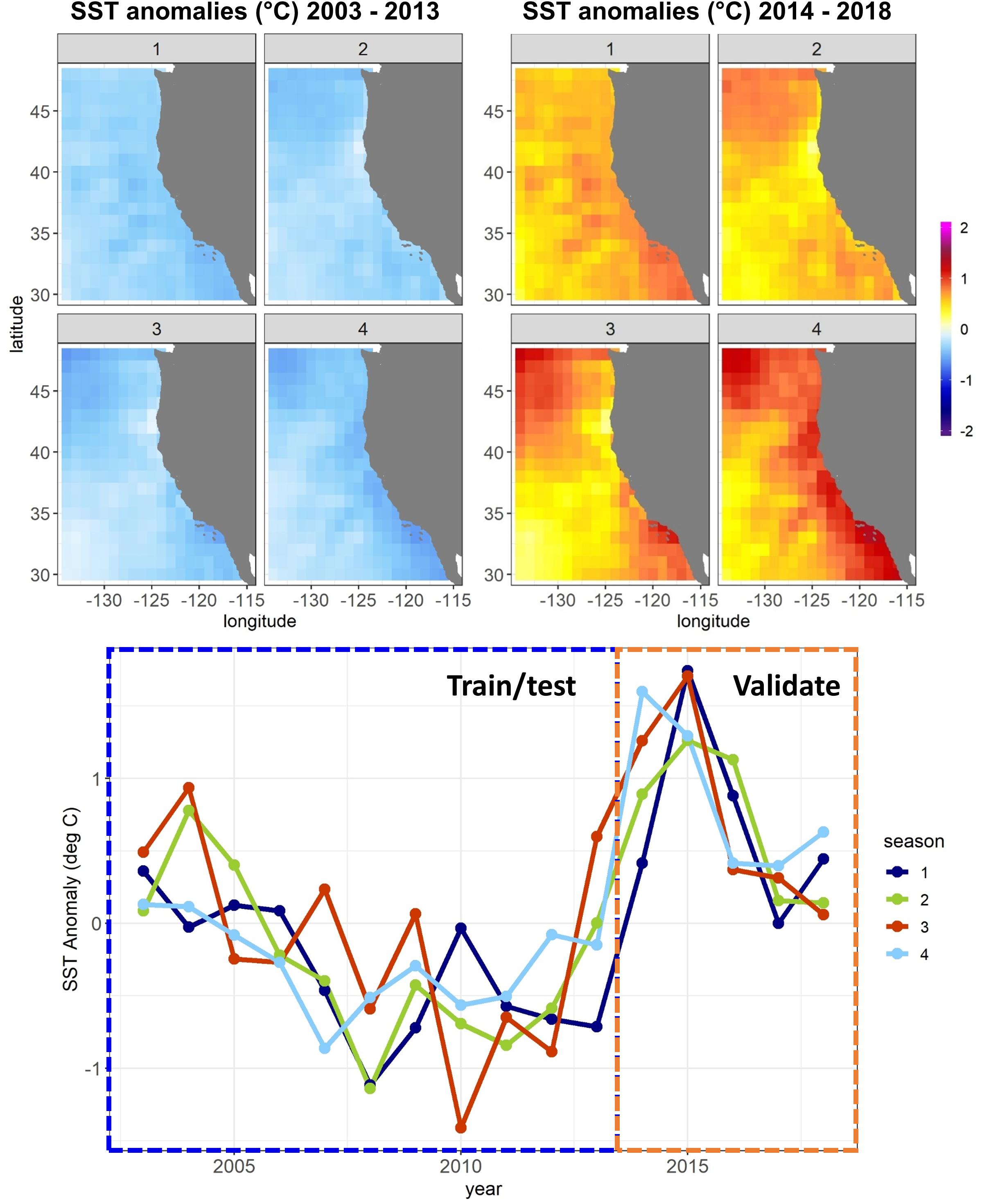
Figure 1. Sea surface temperature (SST) anomalies against a 1980–2018 mean from the CCS ROMS by quarter (January–March, April–June, etc.) for the Experiment 1 SDM training/testing and validation time periods. Anomalies are averaged temporally and mapped spatially at 1° resolution (top) and averaged spatially across the whole model domain and plotted temporally (bottom).

With novel environmental conditions, such as marine heatwaves, becoming increasingly common, there is a critical need to test if our predictions of species responses to these conditions are realistic (Guisan et al., 2013). The CCS marine heatwave can thus provide a useful out-of-sample robustness test for SDMs trained on prior years (Becker et al., 2018). If SDMs can reproduce the anomalous species distributions observed in 2014–2016, it instills confidence in their usefulness as tools for projecting species distributions decades into the future. Conversely, a strong loss of SDM skill during the heatwave years may suggest that the underlying mechanisms driving species distributions in the CCS have not been adequately captured.

Pacific sardine (Sardinops sagax: sardine hereafter) and northern anchovy (Engraulis mordax: anchovy hereafter) are ecologically important forage fish in the CCS, transferring energy from plankton to upper trophic levels (Koehn et al., 2016). Their dynamics are characterized by boom and bust cycles, even in the absence of industrial fishing (Baumgartner, 1992). In the past 10 years, sardine biomass has declined to very low levels, while anchovy abundance has increased strongly since 2017 (Lindegren et al., 2013; Gallo et al., 2019; Thompson et al., 2019; Zwolinski et al., 2019). Anchovy are associated with cool, upwelled waters in shallower coastal environments, and are generally non-migratory (Checkley et al., 2009). The central anchovy subpopulation ranges from Baja California to San Francisco, and spawns off southern and central California, while the northern subpopulation ranges from San Francisco to British Columbia, and spawns near the Columbia River plume (Emmett et al., 2005; Litz et al., 2008; Checkley et al., 2009; Duguid et al., 2019). Sardine reside in warmer, more oligotrophic waters between the California Current and the coastal upwelling region (Checkley et al., 2009). Two of the three sardine subpopulations undergo annual northward feeding migrations, the extent of which may depend on oceanographic conditions, population size, and age structure (Smith, 2005; Zwolinski et al., 2011; McDaniel et al., 2016). The southern subpopulation extends from southern Baja California to southern California, and spawns in summer and fall off southern Baja California. The northern subpopulation, and extends from northern Baja California to British Columbia (Valencia-Gasti et al., 2018), spawning off central and southern California in spring, and in spring-summer off Oregon and Washington in some years (Zwolinski et al., 2011; Auth et al., 2018).

Ongoing research surveys provide extensive distribution information for sardine and anchovy across life stages in the CCS, making them useful case study species. In this study, we thus assessed the ability of five different types of SDM to predict distributions of adults and larvae of sardine and anchovy in the region. Our chosen SDMs spanned a range of complexity from simple, single-variable thermal niche models (TNMs) to more complex machine learning models. We assessed the predictive skill for each SDM across two separate experiments. The first used data collected from 2003 to 2013 to train the SDMs, and then externally validated them against observations from 2014 to 2018, a time period including the 2014–2016 marine heatwave. The second experiment allowed the SDMs to use observations from the marine heatwave years for model training, and validated them against data from withheld years with near-average temperature conditions (2003–2007). We discuss our results in light of current knowledge on the ecology of sardine and anchovy in the CCS, and offer some potential explanations for differences in skill observed between the two experiments and across each life stage of each species.

Materials and Methods

Biological Data Sources

Catch records for adult sardine and anchovy were obtained from trawl surveys conducted by the NOAA Southwest Fisheries Science Center (SWFSC). There were data from 1,777 hauls available for use, from 29 cruises conducted between July 2003 and September 2018. Sampling effort was primarily concentrated in spring (April: 657 hauls) and summer (July–August: 737 hauls), but some data were also available from other months between March and October. The trawl net was towed near the surface at night at a target speed of 3.5–4.0 knots. The net was fitted with an 8 mm mesh liner in the codend (more details are contained in Zwolinski and Demer, 2012; Zwolinski et al., 2012 and Weber et al., 2018). Sampling was concentrated on the continental shelf and slope.

Larval occurrence records for California waters were primarily sourced from the California Cooperative Oceanic Fisheries Investigations (CalCOFI) surveys. Collections under this program began in 1949, and CalCOFI cruises have occupied a standard grid of 66 stations off southern California since 1985. We used catches from standard oblique 0.71 m bongo net tows, which are fitted with 505 mm mesh and towed to 210 m depth (Kramer et al., 1972; Moser et al., 2001; Asch, 2015). Larval occurrence records for the northern California Current were sourced from various sampling programs conducted between 1998 and 2018 by the NOAA Northwest Fisheries Science Center (NWFSC) along the central Oregon coast. These catches derived from 1-m ring and 0.6–0.7 m bongo net tows fitted with 0.200–0.333 mm mesh towed to 20–100 m depth (Auth et al., 2015, 2018; Thompson et al., 2019). Larval data from the entire Oregon and southern Washington coasts were available from yearly (since 2013) NWFSC Prerecruit surveys using a 0.7 m bongo net with 0.333 mm mesh (Brodeur et al., 2019; Thompson et al., 2019).

Environmental Variables

Environmental predictors for the SDMs were sourced from a data assimilative CCS configuration of the Regional Ocean Modeling System (ROMS), with 42 terrain-following vertical levels. The ROMS domain covered from 30 to 48°N, inshore of 134°W at 0.1° horizontal resolution¹ (Veneziani et al., 2009; Neveu et al., 2016). The suite of predictors was the same as used by previous distribution modeling studies for marine vertebrates in the CCS (Scales et al., 2017; Becker et al., 2018; Brodie et al., 2018; Muhling et al., 2019; Smith et al., 2020), and is shown in Table 1. We included SST due to the known importance of temperature to physiological processes and habitat delineation in our species (Checkley et al., 2000; Zwolinski et al., 2011; Weber et al., 2018). Mesoscale oceanographic activity has been shown to delineate favorable spawning areas for small pelagic fishes (Asch and Checkley, 2013), and was captured through sea surface height and eddy kinetic energy. We also included predictors of current flow and wind stress (northward and eastward wind stress, current velocities, wind stress curl), as these are important in shaping retention characteristics and drivers of primary productivity in the region (Jacox et al., 2018). As Brodie et al. (2018) showed the importance of indicators of subsurface water column structure (such as isothermal layer depth and bulk buoyancy frequency) in predicting the distribution of large pelagic fishes and sharks in the CCS, we also included these variables. Isothermal layer depth captures the thickness of the well-mixed surface layer, while bulk buoyancy frequency indicates the stability of the upper water column. The spatial standard deviation of both SST and sea surface height at 0.7° resolution were also included as predictors, to highlight areas of high variability such as frontal zones (Hazen et al., 2018). More information on the calculation of these parameters is available in Brodie et al. (2018) and Muhling et al. (2019). Although surface salinity is available from the ROMS, we chose not to include it as a predictor as it was inconsistent through time, across the two ROMS experiments (1980–2010 and 2011 – present: see Brodie et al., 2018). Values of each ROMS predictor were extracted at native 0.1° spatial resolution, for the date and location of biological sampling. As the CCS ROMS is physics-only (no biogeochemistry), we used satellite surface chlorophyll to approximate primary productivity. These data were obtained from chlorophyll re-analyses developed through the Ocean-Colour Climate Change Initiative (OC-CCI) using multiple ocean color sensors (Sathyendranath et al., 2019). Chlorophyll was extracted at 0.25° spatial resolution, and from 8-day composites overlapping biological sampling dates, to minimize the number of observations lost to cloud cover. Where no 8-day chlorophyll observations were available for a sampling station, we used monthly chlorophyll instead, as the correlation between 8-day and monthly chlorophyll was high (r > 0.8). This impacted <5% of the biological observations. Eddy kinetic energy and surface chlorophyll were both strongly right-skewed, and so were log_e and 4th root transformed, respectively, before inclusion in the SDMs. None of the environmental predictors were linearly correlated with each other at r > 0.6 or r < −0.6, and so all were included in the SDMs.

TABLE 1

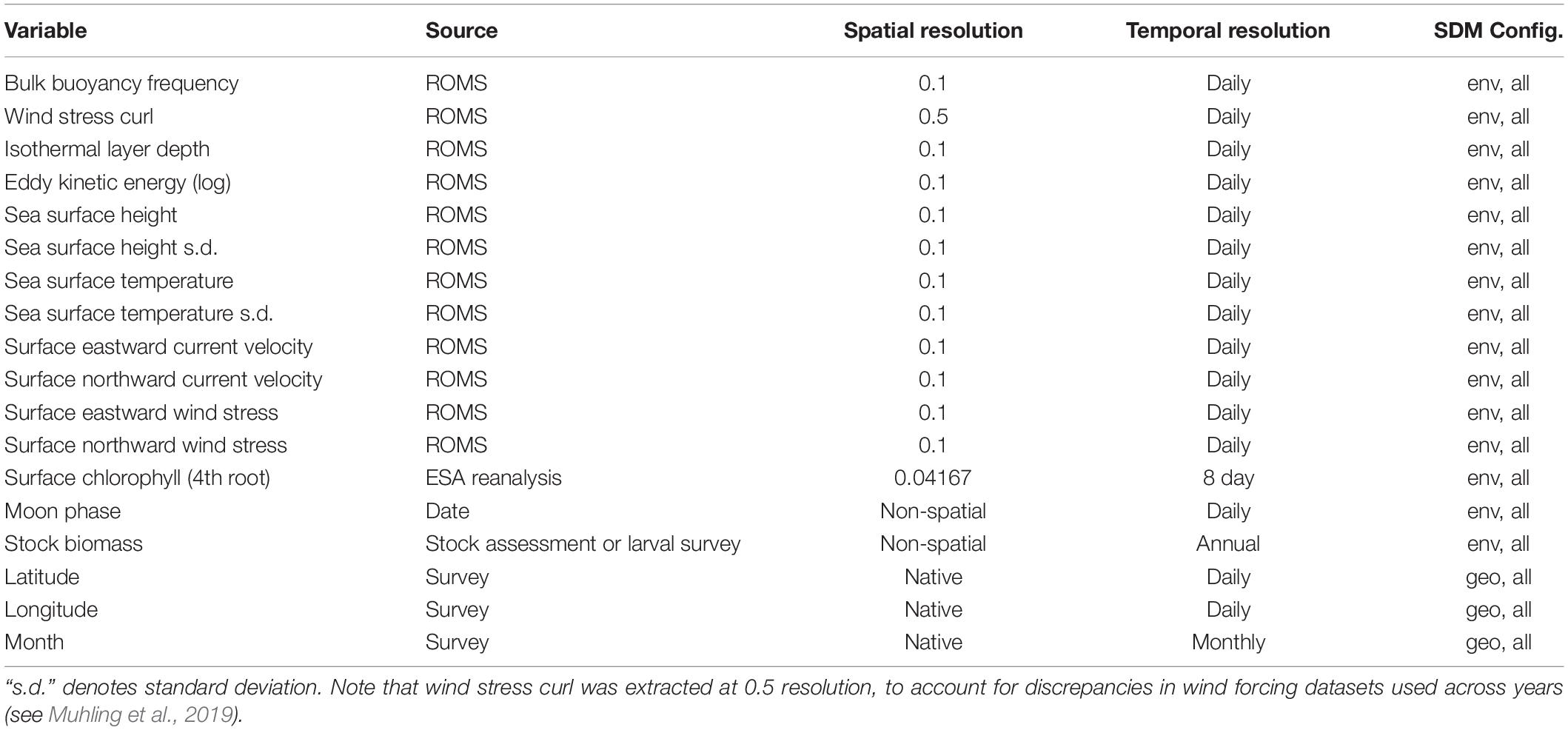
Table 1. Predictors used to build SDMs, and SDM configurations which included each variable.

Following Weber and McClatchie (2010) and Muhling et al. (2019) we included annual biomass indicators as additional predictors for both species, to account for potentially different rates of occupation of environmentally suitable habitat at different stock sizes (Supplementary Figure S1). Previous studies have shown that actual occupied habitat is more spatiotemporally restricted than potential habitat for many fish species, particularly when stock biomass is low (Planque et al., 2007; Reiss et al., 2008). For sardine, we used annual standing stock biomass estimated from sardine stock assessments (Hill et al., 2014, 2018). For anchovy, we used 3-year running mean larval abundances from CalCOFI surveys to index anchovy stock biomass (following Zwolinski and Demer, 2012), as there is no current stock assessment for this species.

Species Distribution Models

All SDMs in this study predicted the probability of occurrence (presence or absence) of each species and life stage. The available biological data from both trawl and larval surveys were split into three sections for use in SDM training, testing, and external validation. Partitioning of observations among these three groups varied across two set experiments, described below.

In Experiment 1, SDMs were trained using a randomly selected 50% of all available observations collected between 2003 and 2013 (training dataset). Optimal SDM configurations were determined based on skill against the other 50% of data from these years (testing dataset). Model skill was quantified using the Area Under the Receiver Operating Characteristic (ROC) curve: (AUC). The AUC metric measures the skill of a classification model. The ROC curve plots the true positive rate against the false positive rate at different classification thresholds, and the area under this curve is used as a measure of model performance. An AUC of 1 indicates a perfect model, where all absences are correctly predicted as absences, and all presences are correctly predicted as presences, while a value of 0.5 indicates that the model’s skill is no better than random. SDMs built using the optimal configuration were then scored against data from years 2014 to 2018 (validation dataset). Results reported for each SDM for each species/life stage thus include (1) a “test” skill, against data not used to build the model but within the same set of years, and (2) a “validation” skill, against data not used to build the model and from a different set of years with novel environmental conditions (Figure 1). To estimate the uncertainty introduced from the random 50% split of 2003–2013 data into training and testing datasets, this split was repeated 10 times (setting the seed each time to allow reproducibility), with optimal SDM configurations re-determined, and a separate set of SDMs saved for each iteration. Mean SDM skill was then assessed across results from all 10 training/testing splits.

Our Experiment 1 training data for the SDMs were restricted to the years 2003–2013, to align with data availability for the trawl surveys. However, larval survey data extend much further back in time. We thus tested two modifications to Experiment 1 for larval sardine and larval anchovy SDMs: the first extended training and testing data back to September 1997, to align with the start of the satellite chlorophyll record. The second modification extended training and testing data back to 1980, to align with the start of the ROMS reanalysis, with chlorophyll dropped as a predictor. Skill against the withheld validation dataset from 2014 to 2018 was then re-tested in the same manner as for the larval SDMs trained using 2003–2013 data.

In Experiment 2, we aimed to assess whether changes in SDM skill between the testing and validation datasets observed in Experiment 1 depended primarily on the novel environmental conditions present during 2014–2018, or on the lack of temporal overlap between the training/testing data and the validation data. The first instance may suggest non-stationarity in relationships between species and their environment during extreme environmental events, or an inability of the SDMs to skillfully extrapolate to novel conditions. The second instance may suggest that the training and testing procedures outlined for Experiment 1 were generally insufficient to prevent overfitting of the SDMs. We thus repeated the SDM training procedure from Experiment 1 but used different splitting criteria. Here, we used 50% of the data from 2008 to 2018 as the training data, and the other 50% as the testing data. Years 2003–2007 were withheld to be used as validation data. In this experiment, the validation data were thus separated from the training/testing data temporally but were not particularly novel environmentally (Figure 1).

As strongly uneven class membership can bias classification models (Kuhn and Johnson, 2013), we used upsampling and downsampling in the caret package (Kuhn et al., 2019) on the training data for both experiments. Downsampling randomly samples the data so that the two classes (positive and negative) end up with the same frequency as the minority class. Upsampling samples the data with replacement to make the two class distributions equal. We upsampled the trawl data, as downsampling resulted in too few observations remaining for model training, but downsampled the much larger larval fish dataset to keep computation times feasible. The most unbalanced training dataset was for adult anchovy in the trawl dataset for Experiment 1 (6.18% positive stations), while the least unbalanced was for adult sardine in the trawl dataset, also for Experiment 1 (33.81% positive stations).

Within each experiment, we tested three subsets of predictors (Table 1 and Figure 2). One set of SDMs was built using all environmental variables plus biomass indicators, longitude, latitude, and month. The next set was built using only environmental predictors and biomass indicators. The last set was built using only longitude, latitude, and month. These three configurations are referred to as “all,” “env,” and “geo,” respectively, throughout the text.

FIGURE 2

Figure 2. Conceptual diagram of SDM ensembles used for each of the two modeling experiments. “GAM” denotes Generalized Additive Models, “BRT” Boosted Regression Trees, “MLP” Multilayer Perceptrons, “RFO” Random Forests, and “TNM” Thermal Niche Models. Note that these ensembles are replicated 10 times for different random splits of the training/testing data.

Five different modeling methods were used to build SDMs for each species/life stage: three machine-learning methods and two forms of Generalized Additive Models (GAMs). These were chosen to represent a range of possible approaches to building SDMs for ecology, and all are well represented in the ecological literature (e.g., Özesmi et al., 2006; Olden et al., 2008; Elith, 2019; Brodie et al., 2020). All SDMs were built in R 3.6.1 (R Core Team, 2019) and are described in more detail below.

Boosted Regression Trees

Boosted Regression Trees (BRTs) are tree-based machine learning models, which are highly flexible and include interactions among predictors implicitly (Elith et al., 2008). BRTs for this study were built using Bernoulli distributions in the dismo and gbm packages (Hijmans et al., 2017; Greenwell et al., 2019). Different combinations of tree complexity, learning rate, and number of trees were tested using the caret package. Tree complexity was allowed to vary between 2 and 5 (with a step of 1), and the number of trees between 1200 and 2400 (step of 40). The best learning rate depends on the tree complexity, number of trees, and number of observations in the training data. We calculated a learning rate coefficient (lr.coeff) based on the number of observations as:

$\begin{array}{c}\hfill \mathrm{lr}.\mathrm{coeff}=1.7\mathrm{e}-06\times \mathrm{n}-1.91\mathrm{e}-04\hfill \end{array}(1)$

where n is the number of observations in the training data. We then allowed the learning rate for BRT training to vary between 4 and 8 times the lr.coeff. We found that this linear equation, determined iteratively, gave a useful range of learning rates to test. Once the “train” function in caret had selected the optimal values for tree complexity, learning rate, and number of trees, 5 BRTs were built using the same training data, to capture the stochasticity in the model building process (Figure 2).

Generalized Additive Models

Generalized Additive Models are semi-parametric regression models which can account for non-linear relationships between covariates and dependent variables using smoothing functions. We built our GAMs in the mgcv package (Wood, 2017). The only parameter tuned for the GAMs was the number of knots (k), which was allowed to vary between 3 and 7, and kept the same for all environmental variables. Although higher values of k can result in slightly more skillful models, this approach can also lead to biologically unreasonable relationships between predictors and dependent variables. Thin plate regression splines were used for all environmental variables, except month, which used a cyclic cubic regression spline. Latitude and longitude were included as a smoothed interaction term, and k was set to the square of the value used for single predictors [i.e., s(lon, lat, k = k × k)]. This approach allowed the GAMs to realistically capture the 2-dimensional spatial structure of the observations (e.g., Zuur, 2012), without overfitting unreasonably in space. The value of k which produced the best AUC on the testing data was selected as optimal. Unlike the machine learning SDMs, multiple GAMs built on the same training data will be identical, and so only one GAM was built for each subset of the training data (Figure 2).

Multilayer Perceptron Artificial Neural Networks

Multilayer Perceptrons (MLPs) are a type of Artificial Neural Network machine learning model (Özesmi et al., 2006). We built our MLPs in the neuralnet package (Fritsch et al., 2019) using the resilient backpropagation with weight backtracking algorithm and a logistic activation function. MLPs were optimized by varying the number of neurons in the single hidden layer between 3 and 10. A maximum possible value of 10 was chosen as although models with >10 neurons sometimes had slightly higher skill against the testing data, they often did not converge, and required much longer computation times to build. Similarly to the BRTs, once an optimal number of neurons was chosen, five MLPs with this configuration were built for each set of the training data.

Random Forests

Random Forest models (RFOs) are also tree-based machine-learning models, but in contrast to BRTs, they use “bagging” (bootstrap aggregating) instead of sequential boosting to create model ensembles (Elith, 2019). We built our RFOs in the randomForest package (Liaw and Wiener, 2002), and optimized the models by varying the number of variables available for splitting at each tree node (“mtry”). This parameter was allowed to vary between a minimum of 2 and a maximum of the number of total predictors. Similarly to the BRTs and MLPs, once the best value of mtry was selected, five RFOs were built for each set of the training data.

Thermal Niche Model

Machine learning SDMs are sometimes criticized for presenting a “black box,” or overly complex approach to distribution modeling (Özesmi et al., 2006; Olden et al., 2008). To examine this perspective for our region and species of interest, we also included a simple TNM in our suite of SDMs. The TNMs were GAMs including only SST as a predictor (and also latitude, longitude, and month for the “all” configuration). The number of knots (k) for SST was fixed at 3, to allow only simple parabolic relationships. Consistent with the approach to building the multivariate GAMs described above, latitude and longitude were included as a smoothed interaction term (except in the “env” configuration), with k set at the same optimal value determined for the full GAM. As with the full GAM, only one TNM was built for each subset of the training data.

Results

Experiment 1: Novel Conditions

Species Distribution Model skill for years 2003–2013 was fair to good (AUCs > 0.7) for all four species/life stage combinations (Figure 3). Skill varied between different covariate configurations, with those containing spatiotemporal predictors (“all” and “geo”) generally outperforming environment-only SDMs (“env”). The exception was adult sardine, where distributions during this time period were generally best predicted using all available environmental and spatiotemporal predictors (“all” configuration), with the spatiotemporal-only SDMs (“geo”) the least skillful and the environment-only SDMs (“env”) showing intermediate skill. In contrast, larval sardine distributions during years 2003–2013 were near equally well predicted by either the “all” or “geo” SDMs, with the “env” SDMs substantially weaker. None of the three SDM configurations consistently outperformed the others for adult anchovy during the SDM training period, although the “env” TNM was particularly weak. This was also the case for sardine larvae and anchovy larvae, suggesting that simple univariate relationships with SST (i.e., the TNM) could not skillfully predict distributions of these species in 2003–2013. Larval anchovy distributions were best predicted by the “all” configuration, but most SDMs built using all three configurations showed good skill (AUCs > 0.75–0.80).

FIGURE 3

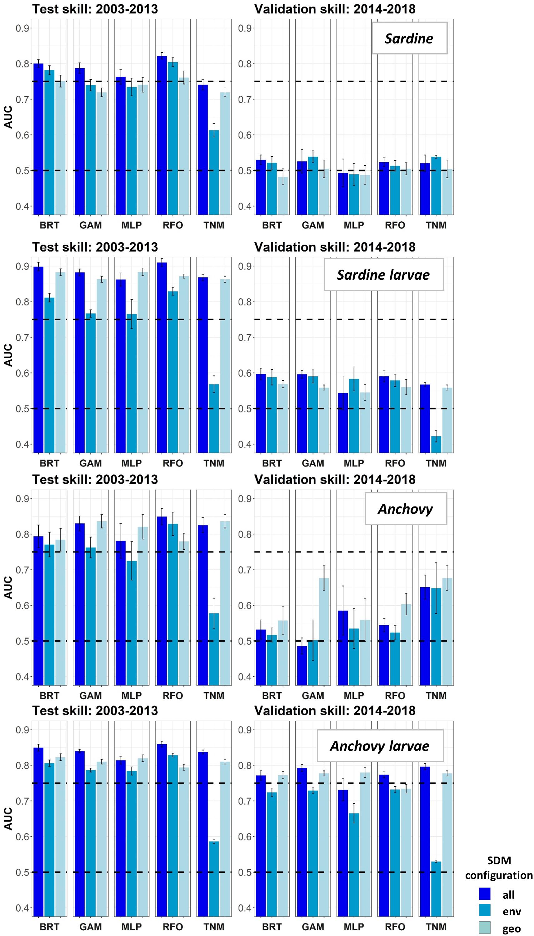
Figure 3. Area Under the Receiver Operating Curve (AUC) skill metrics for Experiment 1 SDMs. Means and standard deviations across all SDM ensembles (see Figure 1) are shown for each life stage of each species. Colors of bars denote the SDM configuration (“all,” “env,” or “geo”). The horizontal black dashed lines show AUC values of 0.5 (no better than a random model), and 0.75 (a rough approximation of a “useful” model), for reference.

In contrast to the results for the SDM training period of 2003–2013, SDM skill for the marine heatwave years of 2014–2018 was markedly lower (Figure 3). AUCs were particularly low for adult sardine, being close to 0.5, or no better than a random model. The TNM for adult anchovy retained some skill, however, mean AUCs were still <0.7. In contrast to the other three species/life stage combinations, the larval anchovy SDMs did retain some skill for years 2014–2018. The “all” and “geo” models generally did the best, suggesting that this result was due to the persistence of previously observed spatiotemporal structure in larval anchovy distributions.

The observed loss of skill for years 2014–2018 was not consistent across seasons. Adult sardine and anchovy SDMs showed improved AUCs (although still <0.75 on average) for the spring period, but much lower skill during summer (Supplementary Figure S2). In contrast, the skill of the larval SDMs was much higher during summer than in spring. In particular, AUCs for the larval sardine BRTs, GAMs and TNMs averaged >0.75 for the “all” configurations during summer, but were generally <0.6 during spring.

The modifications to the Experiment 1 larval SDMs with a longer testing and training time period allowed the SDMs to use records from El Niño years with very warm temperatures in the early 1980s and late 1990s (Figure 4). However, validation skill on data from 2014 to 2018 did not change markedly for either sardine larvae or anchovy larvae depending on the testing and training years used. In fact, SDMs for both taxa showed a slight decline in validation skill when the testing and training data were extended back in time to 1997, and then to 1980.

FIGURE 4

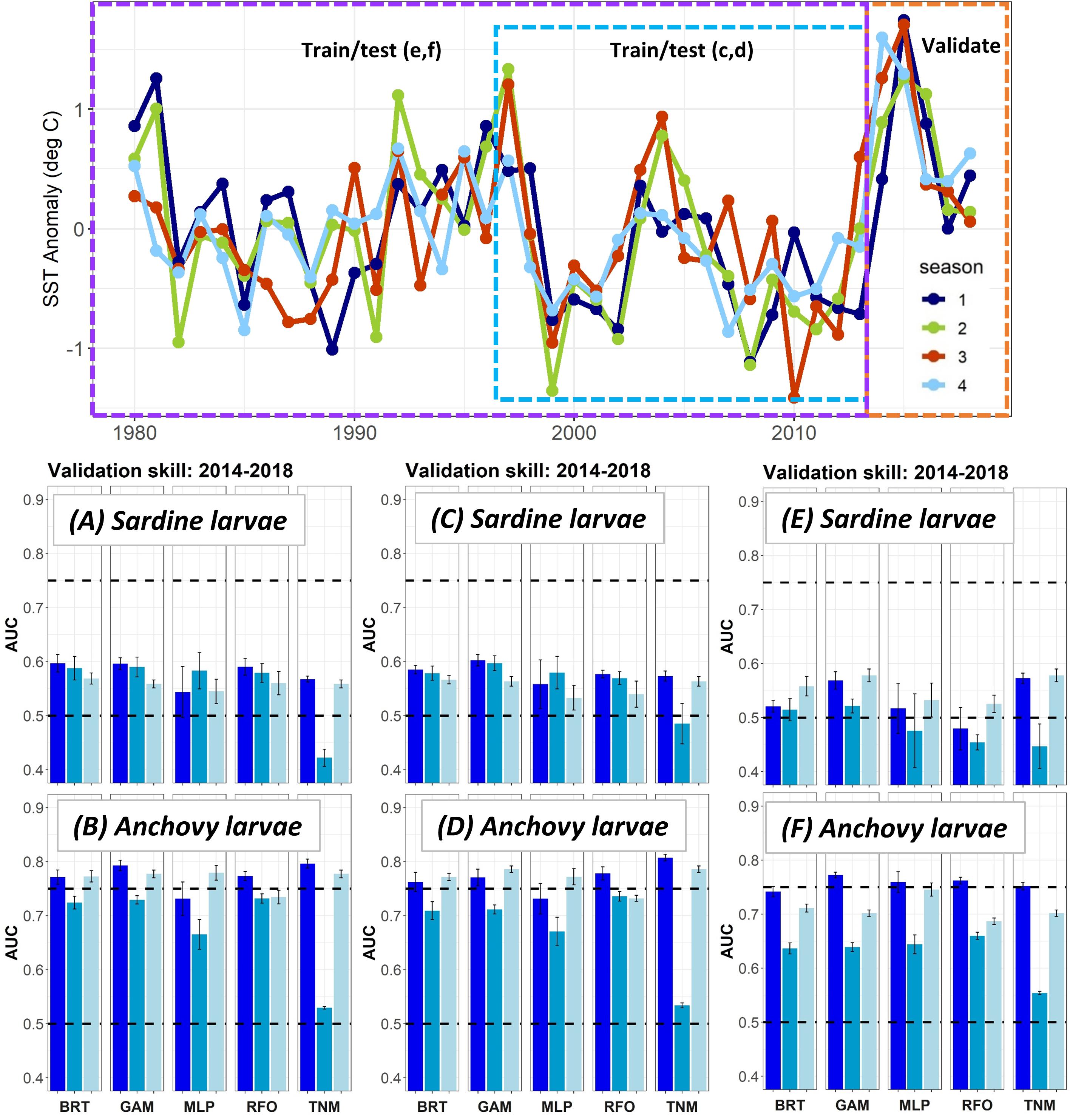
Figure 4. SST anomalies averaged across the ROMS domain from 1980 to 2018 (top), and validation AUCs for years 2014–2018 for larval sardine and larval anchovy SDMs trained using data from (A,B) 2003–2013 (i.e., Experiment 1), (C,D) 1997–2013, (E,F) 1980–2013. Means and standard deviations across all SDM ensembles (see Figure 1) are shown for each life stage of each species. Colors of bars denote the SDM configuration (“all,” “env,” or “geo”). The horizontal black dashed lines show AUC values of 0.5 (no better than a random model), and 0.75 (a rough approximation of a “useful” model), for reference.

None of the five SDM methods consistently out-performed the others across both time periods, for all species/life stage combinations (Figures 3, 4). In particular, the prediction skill for the three machine learning methods was not substantially different to those from the GAMs. The skill of the simple TNM was often weaker during 2003–2013, but it was among the best SDMs for years 2014–2018 for adult sardine, adult anchovy, and larval anchovy.

Two-dimensional representations of SDM predictions were examined by binning observations and SDM predictions by SST and latitude, and averaging probabilities of occurrence within each bin. A comparison of these between the testing and validation time periods suggested some potential drivers of skill loss for the adult sardine SDMs (Figure 5A). During the model training time period (2003–2013), sardine were most likely to be collected where SSTs were between approximately 10 and 18°C, with somewhat higher probabilities of occurrence north of 42°N. This pattern was captured well by the SDMs. During the marine heatwave years, adult sardine were collected roughly within this same SST range in the northern study area, but patterns were much different in the south. Sardine were less likely to be collected south of 40°N at SSTs of 10–15°C than they were previously, but much more likely to be collected where SSTs were >19°C (Figure 5A). This shift was not captured by any of the SDMs, which all assumed very low probabilities of occurrence in these very warm conditions, in line with historical observations. This mismatch is also evident from one-dimensional partial relationships of adult sardine to SST, across all observations and SDMs (Supplementary Figure S3).

FIGURE 5

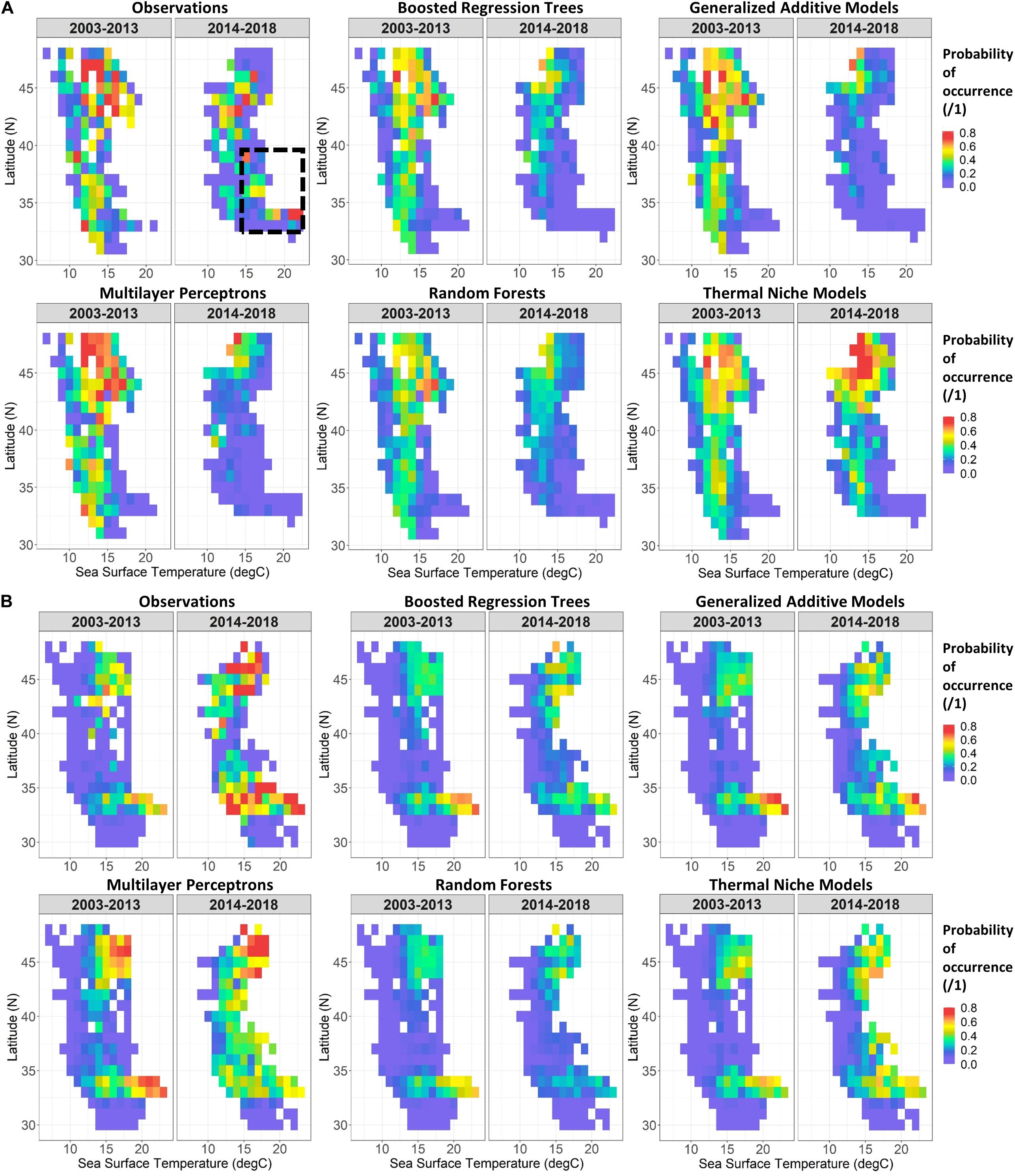
Figure 5. Two-dimensional partial responses of Experiment 1 SDMs for adult sardine (A) and anchovy larvae (B) against SST and latitude, integrated across all other predictors. Predictions from the five SDM types are shown, as well as a summary of observations (mean probabilities of occurrence within 1° SST and latitude bins) for years 2003–2013 (left) and 2014–2018 (right). The black dash box in (A) draws attention to sardine observations from 2014 to 2018 which were poorly predicted by the SDMs.

Two-dimensional representations of larval anchovy SDMs provide a contrast to the adult sardine SDMs (which performed the poorest on the validation dataset). Relationships between larval anchovy and SST with latitude remained much more constant between the training and validation time periods (Figure 5B). Larval anchovy were collected at SSTs of approximately 11–23°C throughout the time series, with two centers of abundance around 33–35°N, and 40–48°N. All of the SDMs captured these patterns well for the training years. While the SDMs were also able to predict the general patterns of distribution in the validation years, all underestimated overall probabilities of occurrence during 2014–2018, particularly at cooler SSTs < 19°C (Figure 5B and Supplementary Figure S3).

A comparison of observations and SDM predictions for two example years with relatively good sampling coverage (2008 and 2015) showed the contrasting responses of both species and life stages to the marine heatwave. Distributions of both adult and larval sardine appeared to move northward during spring 2015 (Figure 6A), although sampling coverage was not as comprehensive as in 2008. In 2008, both adult and larval sardine were concentrated south of 40°N during April and May, coinciding with areas of highest predicted probability from all of the SDMs. In 2015, adult sardine were not common in the trawl surveys, due to their low spawning stock biomass, but those that were present were located between 38 and 44°N. While the SDMs also predicted a northward shift in habitat, these predictions did not align exactly with observations, particularly for the GAMs and MLPs. Similarly, predictions from the larval sardine SDMs suggested a northward shift, but models underestimated the extent of the observed change in larval distributions (Figure 6A). The GAMs and MLPs did show some favorable habitat between 40 and 45°N, where larvae were collected, but also showed favorable habitat off southern California, where sampling collected very few larvae.

FIGURE 6

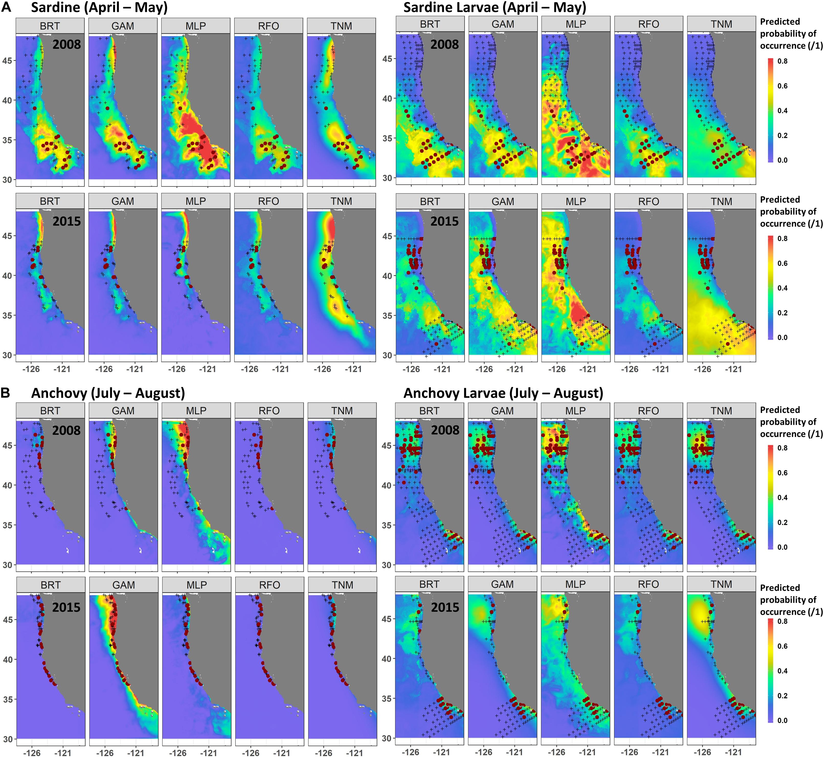
Figure 6. Predicted and observed distributions of sardine and sardine larvae during April–May (A), and anchovy and anchovy larvae during July–August (B), for two examples years. SDM predictions are a mean across Experiment 1 SDM ensembles (see Figure 2). Observed presences are shown in maroon dots, observed absences by black crosses.

In contrast to sardine, adult and larval anchovy did not show strong northward shifts during summer 2015 (Figure 6B). Adult anchovy were present between 37 and 48°N during July and August of both 2008 and 2015. This was captured better by the GAMs than the other SDMs for these particular years. Although larval sampling coverage differed between the years, the two centers of larval anchovy abundance appeared to persist during both 2008 and 2015 (Figure 6B). This persistence occurred despite strongly contrasting environmental conditions between the 2 years (Figure 1). However, while SST was moderately important to the larval anchovy SDMs, it was less influential than latitude and longitude (Supplementary Figure S4). SST was also not a strong contributor to the adult anchovy SDMs. Anchovy thus appeared more likely to maintain their historical spatiotemporal distribution patterns than sardine, partially due to weaker relationships with SST.

The maps in Figures 6A,B suggested that the SDMs often captured some aspects of distribution patterns, but that predictions were not precisely aligned with observations. To test the effect of spatial resolution on SDM skill, we thus aggregated all predictions and observations to 2 × 2°, taking the maximum value of each within each cell. AUCs increased to >0.75 on average for most of the BRTs, GAMs, RFOs, and TNMs for sardine larvae, for the adult anchovy TNMs, and for the “env” GAMs and TNMs for adult sardine using these spatial coarsened data, but remained <0.75 for all other models (results not shown). Collapsing observed and predicted probabilities of occurrence even further, down to means within 2° latitudinal blocks, showed that SDMs were more successful at capturing the general direction of change than the magnitude of change (Figure 7). For example, both the adult and larval sardine SDMs captured the tendency for there to be more sardine in the northern CCS and less in the south during spring, but under-predicted the scales of these shifts. In contrast, the adult anchovy GAMs and MLPs correctly predicted an increase in overall probabilities of occurrence but were unable to reproduce the spatial patterns of these increases. The larval anchovy SDMs correctly predicted the spatial persistence of the two main spawning locations in 2014–2018 and the increase in probabilities of occurrence in the northern CCS (Figures 6B, 7). However, the models were not able to predict the observed increases in probabilities of larval anchovy occurrence in the southern CCS.

FIGURE 7

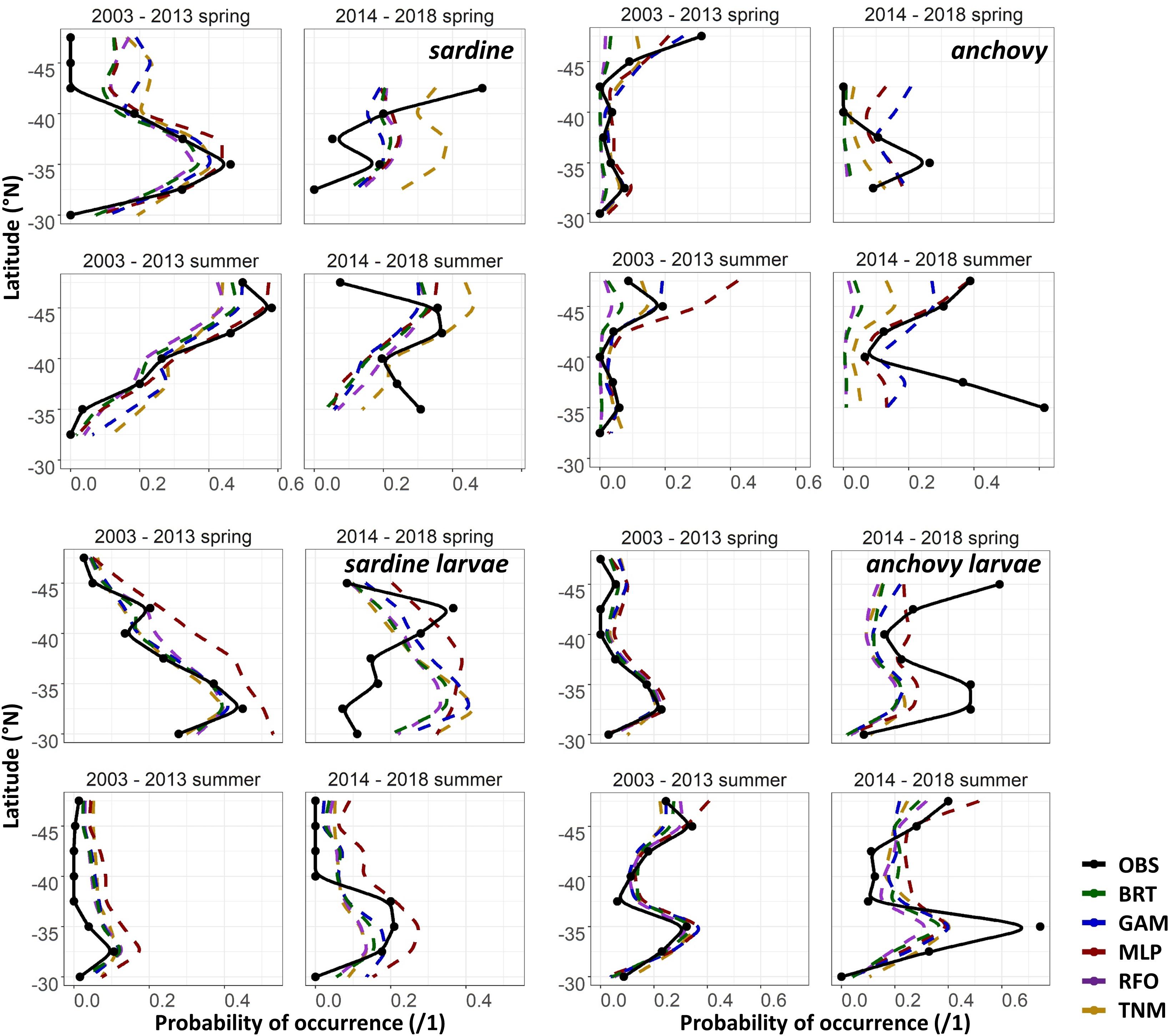
Figure 7. Mean observed (black) and SDM predicted (colors) probabilities of occurrence of each life stage of each species in spring (April–May) and summer (July–August) by 2° latitude bins, for the test (2003–2013) and validation (2014–2018) time periods for Experiment 1.

Sampling coverage during the model training time period (2003–2013) was generally more spatially extensive and covered more negative habitat than during the validation period (2014–2018), a trend evident in Figures 6A,B. To assess the potential impact of this difference on 2014–2018 AUCs, we re-scored data from these years with some “dummy” negative stations added. These negative stations were located at aggregated 1 × 1° locations sampled only during 2003–2013 but not 2014–2018, and where no sardine or anchovy were recorded during the earlier period. Dummy negative stations were calculated and added separately for the trawl and larval datasets, with one station each added for each location in each year (2014–2018) at the end of April, and the end of July, to capture the two best sampled seasons. Environmental data were extracted at these new locations, and re-scored through the SDMs. AUCs for this new dataset including dummy negative stations were generally higher than for the original data (Supplementary Figure S5). This improvement was more marked for adult sardine and anchovy than for larvae, suggesting that lower and more inshore spatial coverage in trawl surveys in recent years may have led to lower AUCs for these life stages. However, the general patterns of skill loss remained consistent, with adult SDMs retaining better skill in spring versus summer, and larval SDMs retaining more skill during summer.

Experiment 2: Near-Average Conditions

Area Under the Receiver Operating Curves for validation years were generally higher in Experiment 2 than for the same taxa and SDMs in Experiment 1 (Figure 8). This result suggested that SDM predictions were more successful in unseen years if the training data covered a more complete range of environmental conditions and/or stock sizes. In particular, larval sardine distributions were well predicted for 2003–2007, in contrast to the strong loss of skill in Experiment 1. The most skillful SDM configurations for larval sardine were “all” and “geo,” suggesting that this skill resulted from SDMs being better able to capture spatiotemporal structure in distributions. Experiment 2 AUCs for withheld validation years also improved for adult sardine and adult anchovy, but mostly remained <0.75. Notably, the adult anchovy SDMs were the only ones to lose substantial skill between the test and validation time periods in Experiment 2. This was partially due to the comparative rarity of anchovy in these earlier years, a result of lower spawning stock biomass and less trawl sampling during summer. Anchovy larvae AUCs for Experiment 2 were slightly weaker than for Experiment 1, but still remained fair to good for all SDMs except for the “env” TNM. These results indicate that the SDMs were largely capable of retaining reasonable skill for years not included in the model training and testing process. The marked loss of skill observed for validation years in Experiment 1 may therefore have resulted mostly from the novel environmental conditions and unexpected species responses to those conditions, rather than SDM overfitting.

FIGURE 8

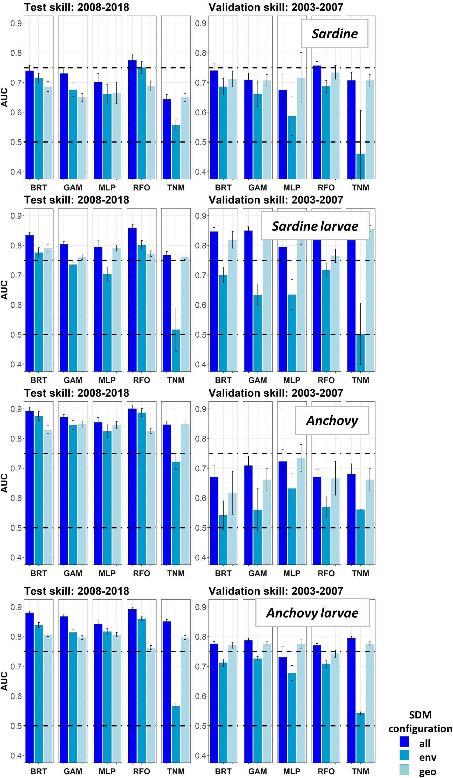
Figure 8. Area Under the Receiver Operating Curve (AUC) skill metrics for Experiment 2 SDMs. Means and standard deviations across all SDM ensembles (see Figure 1) are shown for each life stage of each species. Colors of bars denote the SDM configuration (“all,” “env,” or “geo”). The horizontal black dashed lines show AUC values of 0.5 (no better than a random model), and 0.75 (a rough approximation of a “useful” model), for reference.

To provide a “best case” model comparison against results from Experiments 1 and 2, we lastly re-trained the SDMs using all available data from 2003 to 2018 (50% each for model training and testing, no data withheld for external validation). A comparison of mean AUC by year and SDM type suggested that the RFOs and BRTs were mostly able to maintain good predictive skill throughout the entire time series, as long as they were initially trained on data including observations from the marine heatwave years, and observations across a range of stock sizes (Figure 9). The MLPs, GAMs, and TNMs also showed useful skill in some years for most taxa, but usually performed less skillfully than the BRTs and RFOs, implying that the tree-based SDMs were best able to capture the complex responses of our species to their environment across different environmental regimes. Results from all sets of SDMs together thus indicate that although some of the machine-learning SDMs were flexible enough to maintain reasonable skill both before and during the marine heatwave, most could only do so if they had access to observations from heatwave years during the model training process. Otherwise, the models had no way to anticipate the non-stationary responses of species to anomalously warm temperatures, and lost much of their predictive skill.

FIGURE 9

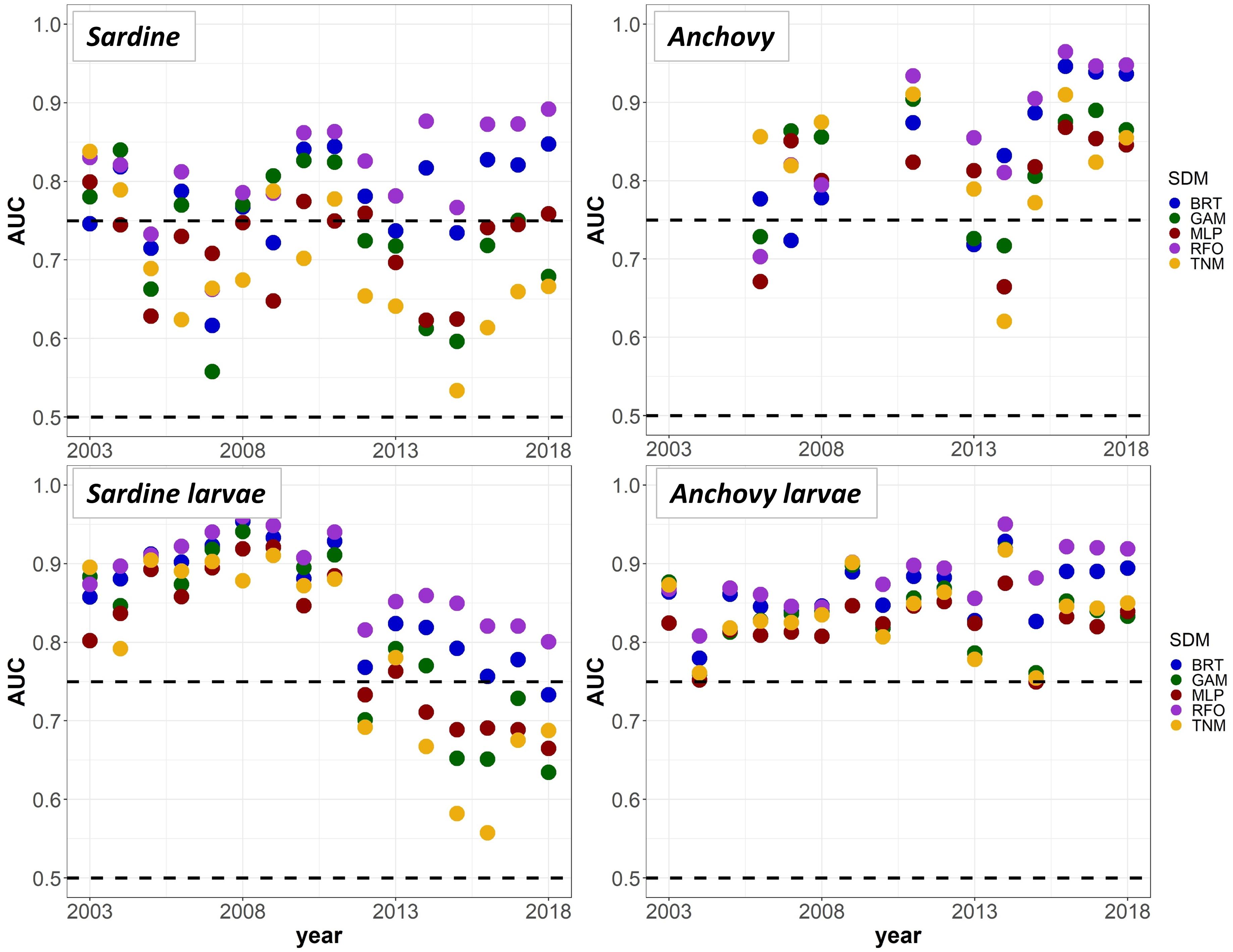
Figure 9. Mean Area Under the Receiver Operating Curve (AUC) test skill metrics for SDMs trained on random 50% splits of all available data from 2003 to 2018, for the “all” covariate configuration only. Colors denote the SDM type. The horizontal black dashed lines show AUC values of 0.5 (no better than a random model), and 0.75 (a rough approximation of a “useful” model), for reference.

Discussion

Our results show that most SDMs lost substantial predictive skill during novel environmental conditions experienced during the recent marine heatwave, regardless of the type of model or the suite of covariates used. However, performance differed among species and life stages. There was no single best type of SDM, although including spatial variables was generally useful. We note that global statistical performance may not always completely represent model value, as some SDMs could capture the general spatial direction of change, even if they could not replicate the observed magnitude.

Importance of Robust SDM Validation

Loss of SDM skill on out-of-model validation datasets is not uncommon, and can be broadly attributed to four issues: (1) model overfitting during training (Elith, 2019), (2) unreasonable model behavior during extrapolation (Hannemann et al., 2015; Beaumont et al., 2016), (3) the selection of irrelevant predictors which do not impact distribution (Steen et al., 2017), and (4) non-stationarity in relationships between a species and its environment (Dormann et al., 2012; Yates et al., 2018). Some degree of over-fitting to the training data may be expected with the more flexible machine learning SDMs used in this study (i.e., BRTs, MLPs, RFOs). However, it was notable that (with the exception of adult anchovy), the GAMs and TNMs showed similarly poor skill to the more complex SDMs for the validation time period. The primary driver of skill loss for years 2014–2018 is thus unlikely to be simply a problem of overfitting in the more complex models. Similarly, the extrapolation behavior of the SDMs to anomalously warm temperatures did not appear to be biologically unreasonable. For example, adult sardine were most commonly collected at SSTs between 9 and 18°C in the Southern California Bight between 2003 and 2013. The SDMs all predicted that this pattern would continue during 2014–2018, and all predicted low probabilities of occurrence where SSTs were warmer than 18°C. In contrast, observations showed that adult sardine were collected with relatively high occurrence in these southern locations, in waters as warm as 21.7°C. These very warm temperatures were rarely sampled between 2003 and 2013.

The third and fourth issues identified above are likely more relevant to our results. Statistical relationships between our species and their environment changed between the model training and validation time periods, particularly for adult sardine. While the relative importance of each predictor to the SDMs frequently varied across model type, all SDMs tended to show similar skill loss during 2014–2018. This suggests that none of the SDMs successfully captured the true drivers of spatial distribution for sardine and anchovy in our study region. The exception was larval anchovy, where the SDMs successfully predicted that the main distribution drivers were environmentally invariant geospatial predictors. However, we note that aggregating observations and predictions to a coarser spatial resolution improved the validation skill of some SDMs to more acceptable levels, and did qualitatively capture the northward shifts in adult and larval sardine distributions during the marine heatwave years. The spatial contraction of sampling effort in recent years may also have led to some relative loss of skill from reduced sampling in strongly negative habitats. In addition, breaking results down by season showed that the larval sardine SDMs performed better during summer, while the adult SDMs showed some improvement in skill during spring. These results suggest that better understanding of spatial processes and spawning phenology should allow the development of more reasonable predictive models in the future.

Our results highlight another important recommendation for the prediction of species distributions, which is the need to validate SDM predictions on an entirely withheld dataset. Results from Experiment 2 show that even when the validation dataset does not include previous unobserved values for environmental predictors (e.g., very warm SSTs), some loss of predictive skill is still possible for some taxa. However, Experiment 2 SDMs (validated against near-average conditions) generally maintained much better skill than those built under Experiment 1 (validated against novel conditions). If there are sufficient observations, the splitting of data into a model training, testing, and external validation set should be standard practice for properly assessing model skill, particularly for the highly flexible machine learning SDMs (Özesmi et al., 2006). This is particularly important if SDMs are to be transferrable to times, locations, or environmental conditions not included within the training data.

Influence of Species Ecology on SDM Performance

Environmental associations of sardine and anchovy in the CCS have been closely studied for more than 50 years (e.g., Lasker and Smith, 1977; Fiedler et al., 1986; Lindegren et al., 2013; Gallo et al., 2019). Extensive previous research suggests that both species have distinct temperature preferences, especially during spawning (Lluch-Belda et al., 1991; Green-Ruiz and Hinojosa-Corona, 1997; Zwolinski et al., 2011; Weber et al., 2018). We may therefore have reasonably expected that both species would respond in a predictable way during the unusual environmental conditions observed in recent years. However, although our results qualitatively captured some of the phenological shifts in spawning recorded by previous studies (e.g., McClatchie et al., 2016; Auth et al., 2018), our SDMs showed a substantial loss of predictive skill across both species and life stages for years 2014–2018, with the exception of larval anchovy.

Relationships between adult sardine and the ocean environment appeared to be especially non-stationary. In particular, none of the SDMs predicted the occurrence of sardine in warm (>18°C) waters during 2014–2018. This observation may be partially due to the increased incursion of adult sardine from the southern sub-stock into United States waters. The current stock assessment uses a SST cutoff rule, where sardine caught at < = 16.7°C are assumed to be from the northern sub-stock and those caught at >16.7°C from the southern sub-stock (Félix-Uraga et al., 2004; García-Morales et al., 2012; Demer and Zwolinski, 2014; Hill et al., 2019). However, re-training and re-validating the adult sardine SDMs only on observations where SST was <16.7°C, to remove the influence of the southern sub-stock, did not improve model validation skill, with all AUCs for 2014–2018 remaining <0.6 (results not shown). Thus, although the low historical sampling coverage in waters warmer than 20°C may have limited the ability of the SDMs to predict to these novel conditions in 2014–2018, relationships between sardine and their environment also changed substantially during the heatwave years even within cooler temperatures. In addition, re-training the larval sardine SDMs using data back to 1980 did not result in more skillful predictions in 2014–2018. These results suggest that distribution patterns and environmental associations for early life stages of sardine during the marine heatwave were unprecedented over the 38 years where larval data were available, despite several strong El Niño events occurring during this timeframe.

In contrast to the other species/life stage combinations, adult sardine SDM skill for both Experiment 2 and for the full models trained on years 2003–2018 mostly remained fair to poor. This result suggests that even when sardine SDMs were able to use observations from the marine heatwave years, they struggled to usefully generalize relationships between this species and its environment. This issue may partially stem from sardine migratory behavior. When biomass is high, the two sardine sub-stocks migrate seasonally. The northern sub-stock moves between southern California in winter and the Pacific Northwest in summer, while the southern sub-stock reaches southern California during summer and returns to coastal Baja California in winter (Lo et al., 2011; Demer et al., 2012). The two sub-stocks thus overlap strongly in space but much less so in time, giving the appearance of largely separate temperature habitats between the two groups. However, laboratory studies show that sardine larvae and adults from both sub-stocks can tolerate very similar, and broad (∼ 9–27°C), thermal ranges if given the opportunity to acclimate (Lasker, 1964; Brewer, 1976; Martínez-Porchas et al., 2009; Pribyl et al., 2016). The strong importance of SST to the sardine SDMs (Supplementary Figure S4) is thus unlikely to represent a purely physiological constraint. Previous studies have also found relationships between sardine and temperature to be complex. For example, McClatchie et al. (2010) showed that a long-standing SST-recruitment relationship for sardine was non-stationary through time, and had reduced predictive skill when applied to more recent data.

During the anomalous conditions of the marine heatwave, adult sardine may also have changed their migration and spawning phenology in response to conditions experienced weeks or months before sampling, leading to observed distribution shifts that did not follow historical environmental associations (see Figure 5A). As older, mature sardine comprise the bulk of the migrant population (Lo et al., 2011; McDaniel et al., 2016), the poor prediction skill during the marine heatwave period may also have been associated with changes in sardine age structure. The 2015–2018 sardine population was not only low in abundance, but trawl acoustic survey data showed younger age classes dominating the age composition (Hill et al., 2019). Younger fish may not have migrated as far north during these years, which may have contributed to the observed latitudinal mismatch between observations and SDM predictions for sardine.

The only species and life stage to retain good skill during the marine heatwave years was larval anchovy. However, this skill derived mostly from the inclusion of geospatial predictors in the SDMs, suggesting that anchovy spawning did not shift markedly in space or time in recent years. This was confirmed by the map comparisons in Figure 6B, showing the spatial persistence of two spawning areas for anchovy in summer during a near-average year (2008) and a heatwave year (2015). This was an unexpected result, as including fixed geospatial predictors in SDMs should theoretically reduce their usefulness for extrapolating to novel environmental conditions. However, previous studies have shown that anchovy in the northern CCS can be associated with the Columbia River plume during warmer months (Emmett et al., 2005; Litz et al., 2008). Spawning anchovy may therefore have maintained their association with this oceanographic feature during the heatwave years, despite the presence of anomalously warm temperatures.

Although the spatial structure of anchovy spawning activity persisted during the marine heatwave, their ability to maintain historical spawning areas under future warming is not clear (e.g., Howard et al., 2020). Climate change is expected to result in mean upper ocean temperature increases of 2–4°C in the CCS by 2100 under the RCP8.5 “business as usual” scenario, with future marine heatwaves leading to even higher SST extremes (Woodworth-Jefcoats et al., 2017; Alexander et al., 2018). While SDMs including geospatial predictors often did better for the marine heatwave test case described in this study, it is probably not reasonable to assume that these relationships will continue to hold decades into the future. Our results therefore highlight the ongoing need for improved mechanistic understanding of movement and distribution drivers for sardine and anchovy in the CCS, if climate change impacts on these species are to be realistically predicted over longer time horizons.

The difficulties inherent to predicting the distributions of migratory species with broad physiological tolerances are also apparent from our results, and have been described for other species previously (e.g., Dambach and Rödder, 2011; Yates et al., 2018). Sardine migratory behavior depends on population size, sub-stock structure, and age composition (Lluch-Belda et al., 1986; Demer et al., 2012; McDaniel et al., 2016). As a result, the presence or absence of sardine and their larvae in the CCS may depend partially on environmental conditions at the time of sampling, and partially on environmental and population drivers of migration and spawning condition earlier in the season. In addition, the same environmental conditions which cause shifts in suitable habitats can also impact recruitment and biomass, which are themselves linked to migration and distribution patterns. During the marine heatwave years, sardine biomass declined to very low levels while anchovy biomass increased sharply (Harvey et al., 2019; Hill et al., 2019). As a result, both environmental conditions and stock biomass for both species during 2014–2018 were outside the ranges of the training period. A combination of both factors, and interactions between them, likely contributed to loss of SDM skill. This is a central problem with using SDMs to predict or project species distributions into the future: it is often more straightforward to anticipate shifts in potential environmental niches than it is to model the complex relationships between stock productivity, movements, and realized habitat use (e.g., Koenigstein et al., 2016).

Other complex factors can drive decoupling of species distributions from their immediate environment, including the persistence of anomalous range extensions even after environmental conditions have returned to normal [e.g., bottlenose dolphin (Tursiops truncatus) off central California: Wells et al., 1990]. Migratory schooling animals may also show inertia in their behaviors deriving from collective memory (Macdonald et al., 2018), or from interactions between environmentally invariant and environmentally responsive movement behaviors (Bauer et al., 2011; Winkler et al., 2014). Taken together, these considerations suggest that caution is required when attempting to use statistical SDMs for future projections of pelagic species habitats. It is worth noting that a similar study predicting marine mammal distributions in the CCS during the 2014–2016 marine heatwave showed higher model skill than we describe here (Becker et al., 2018). Correlative SDMs may therefore still have use for certain climate prediction problems within some ecosystems. Progression toward more mechanistically informed distribution models which incorporate processes such as metabolism, energy budgets, foraging ecology, and migratory behavior can alleviate some of the drawbacks of statistical SDMs (e.g., Lehodey et al., 2008; Planque et al., 2011; Deutsch et al., 2015; Fiechter et al., 2015; Rose et al., 2015; Koenigstein et al., 2016; Howard et al., 2020). However, a sound understanding of physiological drivers across different species is required before the best modeling framework can be identified (Yates et al., 2018), and there are insufficient data available on these processes for many marine taxa.

Conclusion and Recommendations

Overall, our results suggest that statistical relationships defined in correlative SDMs can break down when confronted with novel environmental conditions. This loss of skill was relatively consistent across the five SDMs examined, despite strong differences in model complexity. While a lack of transferability of SDMs in time or space can result from multiple mechanisms (Yates et al., 2018), in our case, the non-stationary responses of our two test species to changes in their ocean environment were particularly influential. Whether the rate of change of the environment contributed to this non-stationarity is unclear (heatwaves represent sudden anomalous change), and validation of long time series would be a valuable test of longer term non-stationarity. Although sardine and anchovy are well-studied forage species in the CCS, their complex environmental associations and behaviors challenged our ability to effectively model their distributions across different oceanographic regimes. Our results thus show the importance of understanding the mechanistic drivers of range shifts in marine species, and the difficulties intrinsic to modeling the distributions of mobile, migratory animals.

We recommend that future work explores methods for including migration and spawning phenology in SDMs for sardine and anchovy in the CCS, for example via correlative SDMs which include spatially remote or time-lagged processes (Thorson et al., 2020), further development of mechanistic models (e.g., Rose et al., 2015), or exploration of hybrid correlative-mechanistic approaches. Development of distribution models by age group, or use of a measure of age composition as an additional covariate may also be beneficial for sardine SDMs. Consistent sampling across a wider range of thermal environments may also allow better definition of potential versus realized habitats for both species. Ultimately, if the SDMs described in this study can be improved to better represent the underlying processes driving distribution shifts in sardine and anchovy, they will be more useful for anticipating the potential impacts of climate change and anomalous environmental events on the future assessment and management of these species, and on the broader CCS.

Data Availability Statement

The CalCOFI larval fish observations are available at: https:// coastwatch.pfeg.noaa.gov/erddap/tabledap/erdCalCOFIlrvcntED toEU.html and https://coastwatch.pfeg.noaa.gov/erddap/tabledap/erdCalCOFIlrvcntQtoSA.html, while the adult trawl survey data are available at: https://coastwatch.pfeg.noaa.gov/erddap/tabledap/FRDCPSTrawlLHHaulCatch.html. Chlorophyll re-analysis fields are also on the Coastwatch ERDDAP server at: https://coastwatch.pfeg.noaa.gov/erddap/griddap/pmlEsaCCI42OceanColor8Day.html. Northern CCS larval survey data are available upon request from author T.D.A. ROMS environmental fields are available upon request by contacting the corresponding author.

Author Contributions

BM, SB, JS, DT, EH, and MJ conceived and designed the study. RB, TA, and CG contributed to data and essential background for the work. BM, SB, JS, CG, DT, EH, MJ, RB, and TA wrote and reviewed the manuscript. BM conducted the statistical analyses and prepared the manuscript figures. All authors contributed to the article and approved the submitted version.

Funding

The authors would like to acknowledge NOAA’s Fisheries and the Environment (FATE) program and Coastal and Ocean Climate Applications (COCA) program for funding portions of this work, including the Future Seas project (grant number NA17OAR4310268) and ongoing data collections in the region.

Disclaimer

The scientific results and conclusions, as well as any views or opinions expressed herein, are those of the author(s) and do not necessarily reflect the views of NOAA or the Department of Commerce.

Conflict of Interest

CG co-founded the company Benchmark Labs.

The remaining authors declare that the research was conducted in the absence of any commercial or financial relationships that could be construed as a potential conflict of interest.

Acknowledgments

We thank the vessels, scientists and crews involved in collecting the biological observations central to this study, as well as Y. Gu and B. Macewicz for data provision. J. Zwolinski, A. Thompson, W. Watson, and Y. Gu provided helpful comments and guidance on data and earlier manuscript drafts. This research was first developed as part of a North Pacific Marine Science Organization (PICES) workshop on “Application of Machine Learning to Ecosystem Change Issues in the North Pacific” convened by C. Hannah, C. Werner, H. Hasumi, and M. St. John in Victoria, BC, Canada October 2019. We also thank the two peer-reviewers for providing helpful feedback which substantially improved the manuscript.

Supplementary Material

The Supplementary Material for this article can be found online at: https://www.frontiersin.org/articles/10.3389/fmars.2020.00589/full#supplementary-material

Footnotes

1. ^ http://oceanmodeling.ucsc.edu/ccsnrt version 2016a

References

Alexander, M. A., Scott, J. D., Friedland, K. D., Mills, K. E., Nye, J. A., Pershing, A. J., et al. (2018). Projected sea surface temperatures over the 21st century: changes in the mean, variability and extremes for large marine ecosystem regions of Northern Oceans. Elementa 6:9. doi: 10.1525/elementa.191

CrossRef Full Text | Google Scholar

Asch, R. G. (2015). Climate change and decadal shifts in the phenology of larval fishes in the California current ecosystem. Proc. Natl. Acad. Sci. U.S.A. 112, E4065–E4074.

Google Scholar

Asch, R. G., and Checkley, D. M. Jr. (2013). Dynamic height: a key variable for identifying the spawning habitat of small pelagic fishes. Deep Sea Res. Part I 71, 79–91. doi: 10.1016/j.dsr.2012.08.006

CrossRef Full Text | Google Scholar

Auth, T. D., Brodeur, R. D., and Peterson, J. O. (2015). Anomalous ichthyoplankton distributions and concentrations in the northern California current during the 2010 El Niño and La Niña events. Prog. Oceanogr. 137, 103–120. doi: 10.1016/j.pocean.2015.05.025

CrossRef Full Text | Google Scholar

Auth, T. D., Daly, E. A., Brodeur, R. D., and Fisher, J. L. (2018). Phenological and distributional shifts in ichthyoplankton associated with recent warming in the northeast Pacific Ocean. Global Change Biol. 24, 259–272. doi: 10.1111/gcb.13872

PubMed Abstract | CrossRef Full Text | Google Scholar

Bauer, S., Nolet, B. A., Giske, J., Chapman, J. W., Åkesson, S., Hedenström, A., et al. (2011). “Cues and decision rules in animal migration,” in Animal Migrations: A Synthesis, eds E. J. Milner-Gulland, J. M. Fryxell, and A. R. E. Sinclair, Chap. 6 (New York: Oxford University Press Inc.), 68–87. doi: 10.1093/acprof:oso/9780199568994.003.0006

CrossRef Full Text | Google Scholar

Baumgartner, T. R. (1992). Reconstruction of the history of the Pacific sardine and northern anchovy populations over the past two millenia from sediments of the Santa Barbara basin, California. Calif. Coop. Oceanic Fish. Invest. Rep. 33, 24–40.

Google Scholar

Beaumont, L. J., Graham, E., Duursma, D. E., Wilson, P. D., Cabrelli, A., Baumgartner, J. B., et al. (2016). Which species distribution models are more (or less) likely to project broad-scale, climate-induced shifts in species ranges? Ecol. Modelling 342, 135–146. doi: 10.1016/j.ecolmodel.2016.10.004

CrossRef Full Text | Google Scholar

Becker, E. A., Forney, K. A., Redfern, J. V., Barlow, J., Jacox, M. G., Roberts, J. J., et al. (2018). Predicting cetacean abundance and distribution in a changing climate. Divers. Distrib. 25, 626–643. doi: 10.1111/ddi.12867

CrossRef Full Text | Google Scholar

Bond, N. A., Cronin, M. F., Freeland, H., and Mantua, N. (2015). Causes and impacts of the 2014 warm anomaly in the NE Pacific. Geophys. Res. Lett. 42, 3414–3420. doi: 10.1002/2015gl063306

CrossRef Full Text | Google Scholar

Brewer, G. D. (1976). Thermal tolerance and resistance of the northern anchovy, Engraulis mordax. Fish. Bull. 74, 433–445.

Google Scholar

Brodeur, R. D., Auth, T. D., and Phillips, A. J. (2019). Major shifts in pelagic micronekton and macrozooplankton community structure in an upwelling ecosystem related to an unprecedented marine heatwave. Front. Mar. Sci. 6:212. doi: 10.3389/fmars.2019.00212

CrossRef Full Text | Google Scholar

Brodie, S., Jacox, M. G., Bograd, S. J., Welch, H., Dewar, H., Scales, K. L., et al. (2018). Integrating dynamic subsurface habitat metrics into species distribution models. Front. Mar. Sci. 5:219. doi: 10.3389/fmars.2018.00219

CrossRef Full Text | Google Scholar

Brodie, S. J., Thorson, J. T., Carroll, G., Hazen, E. L., Bograd, S., Haltuch, M. A., et al. (2020). Trade-offs in covariate selection for species distribution models: a methodological comparison. Ecography 43, 11–24. doi: 10.1111/ecog.04707

CrossRef Full Text | Google Scholar

Buckley, L. B., Urban, M. C., Angilletta, M. J., Crozier, L. G., Rissler, L. J., and Sears, M. W. (2010). Can mechanism inform species’ distribution models? Ecol. Lett. 13, 1041–1054.

Google Scholar

Cavole, L. M., Demko, A. M., Diner, R. E., Giddings, A., Koester, I., Pagniello, C. M., et al. (2016). Biological impacts of the 2013–2015 warm-water anomaly in the Northeast Pacific: winners, losers, and the future. Oceanography 29, 273–285.

Google Scholar

Checkley, D., Ayon, P., Baumgartner, T., Bernal, M., Coetzee, J. C., Emmett, R. L., et al. (2009). “Habitats in Checkley,” in Climate Change and Small Pelagic Fish, eds C. Roy, J. Alheit, Y. Oozeki, and D. Checkley (Cambridge, MA: Cambridge University Press), 12–44.

Google Scholar

Checkley, D. M., Dotson, R. C. Jr., and Grif?th, D. A. (2000). Continuous, underway sampling of eggs of Pacific sardine (Sardinops sagax) and northern anchovy (Engraulis mordax) in spring 1996 and 1997 off southern and central California. Deep Sea Res. Part II 47, 1139–1155. doi: 10.1016/s0967-0645(99)00139-3

CrossRef Full Text | Google Scholar

Cheung, W. W., Brodeur, R. D., Okey, T. A., and Pauly, D. (2015). Projecting future changes in distributions of pelagic fish species of Northeast Pacific shelf seas. Prog. Oceanogr. 130, 19–31. doi: 10.1016/j.pocean.2014.09.003

CrossRef Full Text | Google Scholar

Crozier, L. G., Hendry, A. P., Lawson, P. W., Quinn, T. P., Mantua, N. J., Battin, J., et al. (2008). Potential responses to climate change in organisms with complex life histories: evolution and plasticity in Pacific salmon. Evol. Appl. 1, 252–270. doi: 10.1111/j.1752-4571.2008.00033.x

PubMed Abstract | CrossRef Full Text | Google Scholar

Dambach, J., and Rödder, D. (2011). Applications and future challenges in marine species distribution modeling. Aquat. Conserv. 21, 92–100. doi: 10.1002/aqc.1160

CrossRef Full Text | Google Scholar

Demer, D. A., and Zwolinski, J. P. (2014). Corroboration and refinement of a method for differentiating landings from two stocks of Pacific sardine (Sardinops sagax) in the California current. ICES J. Mar. Sci. 71, 328–335. doi: 10.1093/icesjms/fst135

CrossRef Full Text | Google Scholar

Demer, D. A., Zwolinski, J. P., Byers, K. A., Cutter, G. R., Renfree, J. S., Sessions, T. S., et al. (2012). Prediction and confirmation of seasonal migration of Pacific sardine (Sardinops sagax) in the California current ecosystem. Fish. Bull. 110, 52–70.

Google Scholar

Deutsch, C., Ferrel, A., Seibel, B., Pörtner, H. O., and Huey, R. B. (2015). Climate change tightens a metabolic constraint on marine habitats. Science 348, 1132–1135. doi: 10.1126/science.aaa1605

PubMed Abstract | CrossRef Full Text | Google Scholar

Di Lorenzo, E., and Mantua, N. (2016). Multi-year persistence of the 2014/15 North Pacific marine heatwave. Nat. Clim. Change 6, 1042–1047. doi: 10.1038/nclimate3082

CrossRef Full Text | Google Scholar

Dormann, C. F., Schymanski, S. J., Cabral, J., Chuine, I., Graham, C., Hartig, F., et al. (2012). Correlation and process in species distribution models: bridging a dichotomy. J. Biogeogr. 39, 2119–2131. doi: 10.1111/j.1365-2699.2011.02659.x

CrossRef Full Text | Google Scholar

Duguid, W. D., Boldt, J. L., Chalifour, L., Greene, C. M., Galbraith, M., Hay, D., et al. (2019). Historical fluctuations and recent observations of Northern Anchovy Engraulis mordax in the Salish Sea. Deep Sea Res. Part II Top. Stud. Oceanogr. 159, 22–41. doi: 10.1016/j.dsr2.2018.05.018

CrossRef Full Text | Google Scholar

Elith, J., and Leathwick, J. R. (2009). Species distribution models: ecological explanation and prediction across space and time. Annu. Rev. Ecol. Evol. Syst. 40, 677–697. doi: 10.1146/annurev.ecolsys.110308.120159

CrossRef Full Text | Google Scholar

Elith, J., Leathwick, J. R., and Hastie, T. (2008). A working guide to boosted regression trees. J. Anim. Ecol. 77, 802–813. doi: 10.1111/j.1365-2656.2008.01390.x

PubMed Abstract | CrossRef Full Text | Google Scholar

Elith, J. (2019). “Machine learning, random forests, and boosted regression trees,” in Quantitative Analyses in Wildlife Science, eds L. A. Brennan, A. N. Tri, and B. G. Marcot, Chap. 15 (Baltimore, MD: Johns Hopkins University Press), 281–297.

Google Scholar

Emmett, R. L., Brodeur, R. D., Miller, T. W., Pool, S. S., Krutzikowsky, G. K., Bentley, P. J., et al. (2005). Pacific sardines (Sardinops sagax) abundance, distribution, and ecological relationships in the Pacific Northwest. Calif. Coop. Oceanic Fish. Invest. Rep. 46, 122–143.

Google Scholar

Félix-Uraga, R., Gómez-Muñoz, V. M., Quiñonez-Velazquez, C., Melo-Barrera, F. N., and García-Franco, W. (2004). On the existence of Pacific sardine groups off the west coast of Baja California and southern California. Calif. Coop. Oceanic Fish. Invest. Rep. 45, 146–151.

Google Scholar

Fiechter, J., Rose, K. A., Curchitser, E. N., and Hedstrom, K. S. (2015). The role of environmental controls in determining sardine and anchovy population cycles in the California current: analysis of an end-to-end model. Prog. Oceanogr. 138, 381–398. doi: 10.1016/j.pocean.2014.11.013

CrossRef Full Text | Google Scholar

Fiedler, P. C., Methot, R. D., and Hewitt, R. P. (1986). Effects of California El Niño 1982–1984 on the northern anchovy. J. Mar. Res. 44, 317–338.

Google Scholar

Fritsch, S., Guenther, F., and Wright, M. N. (2019). neuralnet: Training of Neural Networks. R Package Version 1.44.2. Avaliable at: https://CRAN.R-project.org/package=neuralnet. (accessed February 07, 2019).

Google Scholar

Gallo, N. D., Drenkard, E., Thompson, A. R., Weber, E. D., Wilson-Vandenberg, D., McClatchie, S., et al. (2019). Bridging from monitoring to solutions-based thinking: Lessons from CalCOFI for understanding and adapting to marine climate change impacts. Front. Mar. Sci. 6:695. doi: 10.3389/fmars.2019.00695

CrossRef Full Text | Google Scholar

García-Morales, R., Shirasago-German, B., Félix-Uraga, R., and Pérez-Lezama, E. L. (2012). Conceptual models of Pacific sardine distribution in the California current System. Curr. Dev. Oceanogr. 5, 23–47.

Google Scholar

Gentemann, C. L., Fewings, M. R., and García-Reyes, M. (2017). Satellite sea surface temperatures along the West Coast of the United States during the 2014–2016 northeast Pacific marine heat wave. Geophys. Res. Lett. 44, 312–319. doi: 10.1002/2016gl071039

CrossRef Full Text | Google Scholar

Green-Ruiz, Y. A., and Hinojosa-Corona, A. (1997). Study of the spawning area of the Northern anchovy in the Gulf of California from 1990 to 1994, using satellite images of sea surface temperatures. J. Plankton Res. 19, 957–968. doi: 10.1093/plankt/19.8.957

CrossRef Full Text | Google Scholar

Greenwell, B., Boehmke, B., and Cunningham, J., and GBM Developers (2019). gbm: Generalized Boosted Regression Models. R Package Version 2.1.5. Avaliable at: https://CRAN.R-project.org/package=gbm (accessed January 14, 2019).

Google Scholar

Guisan, A., Tingley, R., Baumgartner, J. B., Naujokaitis-Lewis, I., Sutcliffe, P. R., and Tulloch, A. I. (2013). Predicting species distributions for conservation decisions. Ecol. Lett. 16, 1424–1435.

Google Scholar

Guisan, A., and Zimmermann, N. E. (2000). Predictive habitat distribution models in ecology. Ecol. Modelling 135, 147–186. doi: 10.1016/s0304-3800(00)00354-9

CrossRef Full Text | Google Scholar

Hannemann, H., Willis, K. J., and Macias-Fauria, M. (2015). The devil is in the detail: unstable response functions in species distribution models challenge bulk ensemble modelling. Global Ecol. Biogeogr. 25, 26–35. doi: 10.1111/geb.12381

CrossRef Full Text | Google Scholar

Harvey, C., Garfield, N., Williams, G., Tolimieri, N., Schroeder, I., Andrews, K., et al. (2019). Ecosystem Status Report of the California Current for 2019: A Summary of Ecosystem Indicators Compiled by the California Current Integrated Ecosystem Assessment Team (CCEIA). Washington, DC: U.S. Department of Commerce, 149.

Google Scholar

Hazen, E. L., Scales, K. L., Maxwell, S. M., Briscoe, D. K., Welch, H., Bograd, S. J., et al. (2018). A dynamic ocean management tool to reduce bycatch and support sustainable fisheries. Sci. Adv. 4:eaar3001. doi: 10.1126/sciadv.aar3001

PubMed Abstract | CrossRef Full Text | Google Scholar

Hijmans, R. J., Phillips, S., Leathwick, J., and Elith, J. (2017). dismo: Species Distribution Modeling. R Package Version 1.1-4. Avaliable at: https://CRAN.R-project.org/package=dismo (accessed January 09, 2017).

Google Scholar

Hill, K. T., Crone, P. R., Demer, D. A., Zwolinski, J., Dorval, E., and Macewicz, B. J. (2014). “Assessment of the Pacific sardine resource in 2014 for US management in 2014-15,” in National Oceanic and Atmospheric Administration Technical Memorandum NMFS-SWFSC-531, (Washington, DC: US Department of Commerce).

Google Scholar

Hill, K. T., Crone, P. R., and Zwolinski, J. P. (2018). “Assessment of the Pacific sardine resource in 2018 for US management in 2018-19,” in National Oceanic and Atmospheric Administration Technical Memorandum NMFS-SWFSC-600, (Washington, DC: US Department of Commerce).

Google Scholar

Hill, K. T., Crone, P. R., and Zwolinski, J. P. (2019). “Assessment of the Pacific sardine resource in 2019 for US management in 2019-20,” in National Oceanic and Atmospheric Administration Technical Memorandum NMFS-SWFSC-615, (Washington, DC: US Department of Commerce).

Google Scholar

Hobday, A. J., Oliver, E. C., Gupta, A. S., Benthuysen, J. A., Burrows, M. T., Donat, M. G., et al. (2018). Categorizing and naming marine heatwaves. Oceanography 31, 162–173.

Google Scholar

Holbrook, N. J., Scannell, H. A., Gupta, A. S., Benthuysen, J. A., Feng, M., Oliver, E. C., et al. (2019). A global assessment of marine heatwaves and their drivers. Nat. Commun. 10, 1–13.

Google Scholar

Howard, E. M., Penn, J. L., Frenzel, H., Seibel, B. A., Bianchi, D., Renault, L., et al. (2020). Climate-driven aerobic habitat loss in the California current system. Sci. Adv. 6:eaay3188. doi: 10.1126/sciadv.aay3188

PubMed Abstract | CrossRef Full Text | Google Scholar

Jacox, M. G. (2019). Marine heatwaves in a changing climate. Nature 571, 485–487. doi: 10.1038/d41586-019-02196-1

PubMed Abstract | CrossRef Full Text | Google Scholar

Jacox, M. G., Edwards, C. A., Hazen, E. L., and Bograd, S. J. (2018). Coastal upwelling revisited: ekman, Bakun and improved upwelling indices for the U.S. West Coast. J. Geophys. Res. 123, 7332–7350. doi: 10.1029/2018jc014187

CrossRef Full Text | Google Scholar

Jacox, M. G., Hazen, E. L., Zaba, K. D., Rudnick, D. L., Edwards, C. A., Moore, A. M., et al. (2016). Impacts of the 2015–2016 El Niño on the California current system: early assessment and comparison to past events. Geophys. Res. Lett. 43, 7072–7080. doi: 10.1002/2016gl069716

CrossRef Full Text | Google Scholar

Johnson, J. E., and Welch, D. J. (2009). Marine fisheries management in a changing climate: a review of vulnerability and future options. Rev. Fish. Sci. 18, 106–124. doi: 10.1080/10641260903434557

CrossRef Full Text | Google Scholar

Kahru, M., Jacox, M. G., and Ohman, M. D. (2018). CCE1: decrease in the frequency of oceanic fronts and surface chlorophyll concentration in the California current system during the 2014–2016 northeast Pacific warm anomalies. Deep Sea Res. Part I Oceanogr. Res. Pap. 140, 4–13. doi: 10.1016/j.dsr.2018.04.007

CrossRef Full Text | Google Scholar

Karp, M. A., Peterson, J. O., Lynch, P. D., Griffis, R. B., Adams, C. F., Arnold, W. S., et al. (2019). Accounting for shifting distributions and changing productivity in the development of scientific advice for fishery management. ICES J. Mar. Sci. 76, 1305–1315.

Google Scholar

Kleisner, K. M., Fogarty, M. J., McGee, S., Hare, J. A., Moret, S., Perretti, C. T., et al. (2017). Marine species distribution shifts on the US Northeast Continental Shelf under continued ocean warming. Prog. Oceanogr. 153, 24–36. doi: 10.1016/j.pocean.2017.04.001

CrossRef Full Text | Google Scholar

Koehn, L. E., Essington, T. E., Marshall, K. N., Kaplan, I. C., Sydeman, W. J., Szoboszlai, A. I., et al. (2016). Developing a high taxonomic resolution food web model to assess the functional role of forage fish in the California current ecosystem. Ecol. Modelling 335, 87–100. doi: 10.1016/j.ecolmodel.2016.05.010

CrossRef Full Text | Google Scholar

Koenigstein, S., Mark, F. C., Gößling-Reisemann, S., Reuter, H., and Pörtner, H. O. (2016). Modeling climate change impacts on marine fish populations: process-based integration of ocean warming, acidification and other environmental drivers. Fish Fish. 17, 972–1004. doi: 10.1111/faf.12155

CrossRef Full Text | Google Scholar

Kramer, D., Kalin, M. J., Stevens, E. G., Thrailkill, J. R., and Zweifel, J. R. (1972). “Collecting and processing data on fish eggs and larvae in the California current region,” in National Oceanic and Atmospheric Administration Technical Report NMFS-CIRC-370, Vol. 370, (Seattle, WA: US Department of Commerce).

Google Scholar

Kuhn, M., and Johnson, K. (2013). Remedies for Severe Class Imbalance. In: Applied Predictive Modeling. New York, NY: Springer.

Google Scholar

Kuhn, M., Wing, J., Weston, S., Williams, A., Keefer, C., Engelhardt, A., et al. (2019). caret: Classification and Regression Training. R Package Version 6.0-84. Avalaiable at: https://CRAN.R-project.org/package=caret (accessed March 20, 2020).

Google Scholar

Lasker, R. (1964). An experimental study of the effect of temperature on the incubation time, development, and growth of Pacific sardine embryos and larvae. Copeia 2, 399–405.

Google Scholar

Lasker, R., and Smith, P. E. (1977). Estimation of the effects of environmental variations on the eggs and larvae of the northern anchovy. Calif. Coop. Oceanic Fish. Invest. Rep. 19, 128–137.

Google Scholar

Lehodey, P., Senina, I., and Murtugudde, R. (2008). A spatial ecosystem and populations dynamics model (SEAPODYM)–Modeling of tuna and tuna-like populations. Prog. Oceanogr. 78, 304–318. doi: 10.1016/j.pocean.2008.06.004

CrossRef Full Text | Google Scholar

Liaw, A., and Wiener, M. (2002). Classification and Regression by randomForest. R News 2, 18–22.

Google Scholar

Lima, F. P., and Wethey, D. S. (2012). Three decades of high-resolution coastal sea surface temperatures reveal more than warming. Nat. Commun. 3, 1–13.

Google Scholar

Lindegren, M., Checkley, D. M., Rouyer, T., MacCall, A. D., and Stenseth, N. C. (2013). Climate, fishing, and fluctuations of sardine and anchovy in the California current. Proc. Natl. Acad. Sci. U.S.A. 110, 13672–13677. doi: 10.1073/pnas.1305733110

PubMed Abstract | CrossRef Full Text | Google Scholar

Link, J. S., Nye, J. A., and Hare, J. A. (2011). Guidelines for incorporating fish distribution shifts into a fisheries management context. Fish Fish. 12, 461–469. doi: 10.1111/j.1467-2979.2010.00398.x

CrossRef Full Text | Google Scholar

Litz, M. N., Heppell, S. S., Emmett, R. L., and Brodeur, R. D. (2008). Ecology and distribution of the northern subpopulation of northern anchovy (Engraulis mordax) off the US west coast. Cali. Coop. Oceanic Fish. Invest. Rep. 49, 167–182.

Google Scholar

Lluch-Belda, D., Lluch-Cota, D. B., Hernandez-Vazquez, S., Salinas-Zavala, C. A., and Schwartzlose, R. A. (1991). Sardine and anchovy spawning as related to temperature and upwell in the California current system. Calif. Coop. Oceanic Fish. Invest. Rep. 32, 105–111.

Google Scholar

Lluch-Belda, D., Magallón, F. J., and Schwartzlose, R. A. (1986). Large fluctuations in the sardine fishery in the Gulf of California: possible causes. Calif. Coop. Oceanic Fish. Invest. Rep. 27, 136–140.

Google Scholar

Lo, N. C., Macewicz, B. J., and Griffith, D. A. (2011). Migration of Pacific sardine (Sardinops sagax) off the west coast of United States in 2003–2005. Bull. Mar. Sci. 87, 395–412. doi: 10.5343/bms.2010.1077

CrossRef Full Text | Google Scholar

Macdonald, J. I., Logemann, K., Krainski, E. T., Sigurðsson, b, Beale, C. M., Huse, G., et al. (2018). Can collective memories shape fish distributions? A test, linking space-time occurrence models and population demographics. Ecography 41, 938–957. doi: 10.1111/ecog.03098

CrossRef Full Text | Google Scholar

Martínez-Porchas, M., Hernández-Rodríguez, M., and Bückle-Ramírez, L. F. (2009). Thermal behavior of the Pacific sardine (Sardinops sagax) acclimated to different thermal cycles. J. Thermal Biol. 34, 372–376. doi: 10.1016/j.jtherbio.2009.07.002

CrossRef Full Text | Google Scholar

McClatchie, S., Goericke, R., Auad, G., and Hill, K. (2010). Re-assessment of the stock-recruit and temperature-recruit relationships for Pacific sardine (Sardinops sagax). Can. J. Fish. Aquat. Sci. 67, 1782–1790. doi: 10.1139/f10-101

CrossRef Full Text | Google Scholar

McClatchie, S., Goericke, R., Leising, A., Auth, T. D., Bjorkstedt, E., Robertson, R. R., et al. (2016). State of the California current 2015-16: comparisons with the 1997-98 El Niño. Calif. Coop. Oceanic Fish. Invest. 57, 1–57.

Google Scholar

McDaniel, J., Piner, K., Lee, H. H., and Hill, K. (2016). Evidence that the migration of the northern subpopulation of Pacific sardine (Sardinops sagax) off the west coast of the United States is age-based. PLoS One 11:e0166780. doi: 10.1371/journal.pone.0166780

PubMed Abstract | CrossRef Full Text | Google Scholar

Mills, K. E., Pershing, A. J., Brown, C. J., Chen, Y., Chiang, F. S., Holland, D. S., et al. (2013). Fisheries management in a changing climate: lessons from the 2012 ocean heat wave in the Northwest Atlantic. Oceanography 26, 191–195.

Google Scholar

Moser, H. G., Charter, R. L., Smith, P. E., Ambrose, D. A., Watson, W., Charter, S. R., et al. (2001). Distributional atlas of fish larvae and eggs in the Southern California Bight region, 1951-1998. Calif. Coop. Oceanic Fish. Invest. Atlas 34:166.

Google Scholar

Muhling, B. A., Brodie, S., Jacox, M., Snodgrass, O., Dewar, H., Tommasi, D., et al. (2019). Dynamic habitat use of albacore and their primary prey species in the California current system. Calif. Coop. Oceanic Fish. Invest. Rep. 60, 1–15.

Google Scholar

Neveu, E., Moore, A. M., Edwards, C. A., Fiechter, J., Drake, P., Crawford, W. J., et al. (2016). An historical analysis of the California current circulation using ROMS 4D-Var: system configuration and diagnostics. Ocean Modelling 99, 133–151. doi: 10.1016/j.ocemod.2015.11.012

CrossRef Full Text | Google Scholar

Norberg, A., Abrego, N., Blanchet, F. G., Adler, F. R., Anderson, B. J., Anttila, J., et al. (2019). A comprehensive evaluation of predictive performance of 33 species distribution models at species and community levels. Ecol. Monogr. 89:e01370.

Google Scholar

Olden, J. D., Lawler, J. J., and Poff, N. L. (2008). Machine learning methods without tears: a primer for ecologists. Q. Rev. Biol. 83, 171–193. doi: 10.1086/587826

PubMed Abstract | CrossRef Full Text | Google Scholar

Özesmi, S. L., Tan, C. O., and Özesmi, U. (2006). Methodological issues in building, training, and testing artificial neural networks in ecological applications. Ecol. Modelling 195, 83–93. doi: 10.1016/j.ecolmodel.2005.11.012

CrossRef Full Text | Google Scholar

Planque, B., Bellier, E., and Lazure, P. (2007). Modelling potential spawning habitat of sardine (Sardina pilchardus) and anchovy(Engraulis encrasicolus) in the Bay of Biscay). Fish. Oceanogr. 16, 16–30. doi: 10.1111/j.1365-2419.2006.00411.x

CrossRef Full Text | Google Scholar

Planque, B., Loots, C., Petitgas, P., Lindstrøm, U. L. F., and Vaz, S. (2011). Understanding what controls the spatial distribution of fish populations using a multi-model approach. Fish. Oceanogr. 20, 1–17. doi: 10.1111/j.1365-2419.2010.00546.x

CrossRef Full Text | Google Scholar

Poloczanska, E. S., Brown, C. J., Sydeman, W. J., Kiessling, W., Schoeman, D. S., Moore, P. J., et al. (2013). Global imprint of climate change on marine life. Nat. Clim. Change 3, 919–925.

Google Scholar

Pribyl, A. L., Hyde, J. R., Robertson, L., and Vetter, R. (2016). Defining an ideal temperature range for the northern subpopulation of Pacific sardine, Sardinops sagax caeruleus. Environ. Biol. Fish 99, 275–291. doi: 10.1007/s10641-016-0473-1

CrossRef Full Text | Google Scholar

Punt, A. E., A’mar, T., Bond, N. A., Butterworth, D. S., de Moor, C. L., De Oliveira, J. A., et al. (2013). Fisheries management under climate and environmental uncertainty: control rules and performance simulation. ICES J. Mar. Sci. 71, 2208–2220. doi: 10.1093/icesjms/fst057

CrossRef Full Text | Google Scholar

R Core Team (2019). R: A Language and Environment for Statistical Computing. Vienna: R Foundation for Statistical Computing.

Google Scholar

Reiss, C. S., Checkley, D. M. Jr., and Bograd, S. J. (2008). Remotely sensed spawning habitat of Pacific sardine (Sardinops sagax) and Northern anchovy (Engraulis mordax) within the California current. Fish. Oceanogr. 17, 126–136. doi: 10.1111/j.1365-2419.2008.00469.x

CrossRef Full Text | Google Scholar

Rose, K. A., Fiechter, J., Curchitser, E. N., Hedstrom, K., Bernal, M., Creekmore, S., et al. (2015). Demonstration of a fully-coupled end-to-end model for small pelagic fish using sardine and anchovy in the California current. Prog. Oceanogr. 138, 348–380. doi: 10.1016/j.pocean.2015.01.012

CrossRef Full Text | Google Scholar

Sakuma, K. M., Field, J. C., Mantua, N. J., Ralston, S., Marinovic, B. B., and Carrion, C. N. (2016). Anomalous epipelagic micronekton assemblage patterns in the neritic waters of the California current in spring 2015 during a period of extreme ocean conditions. Calif. Coop. Oceanic Fish. Invest. Rep. 57, 163–183.

Google Scholar

Sathyendranath, S., Brewin, R. J., Brockmann, C., Brotas, V., Calton, B., Chuprin, A., et al. (2019). An ocean-colour time series for use in climate studies: the experience of the ocean-colour climate change initiative (OC-CCI). Sensors 19:4285. doi: 10.3390/s19194285

PubMed Abstract | CrossRef Full Text | Google Scholar

Scales, K. L., Hazen, E. L., Maxwell, S. M., Dewar, H., Kohin, S., Jacox, M. G., et al. (2017). Fit to predict? Eco-informatics for predicting the catchability of a pelagic fish in near real time. Ecol. Appl. 27, 2313–2329. doi: 10.1002/eap.1610

PubMed Abstract | CrossRef Full Text | Google Scholar

Silber, G. K., Lettrich, M. D., Thomas, P. O., Baker, J. D., Baumgartner, M., Becker, E. A., et al. (2017). Projecting marine mammal distribution in a changing climate. Front. Mar. Sci. 4:413. doi: 10.3389/fmars.2017.00413

CrossRef Full Text | Google Scholar

Smale, D. A., Wernberg, T., Oliver, E. C., Thomsen, M., Harvey, B. P., Straub, S. C., et al. (2019). Marine heatwaves threaten global biodiversity and the provision of ecosystem services. Nat. Clim. Change 9, 306–312. doi: 10.1038/s41558-019-0412-1

CrossRef Full Text | Google Scholar

Smith, J. A., Tommasi, D., Sweeney, J., Brodie, S., Welch, H., Hazen, E. L., et al. (2020). Lost opportunity: quantifying the dynamic economic impact of time-area fishery closures. J. Appl. Ecol. 57, 502–513. doi: 10.1111/1365-2664.13565

CrossRef Full Text | Google Scholar

Smith, P. E. (2005). A history of proposals for subpopulation structure in the Pacific sardine (Sardinops sagax) population off western North America. Calif. Coop. Oceanic Fish. Invest. Rep. 46:75.

Google Scholar

Steen, V., Sofaer, H. R., Skagen, S. K., Ray, A. J., and Noon, B. R. (2017). Projecting species’ vulnerability to climate change: which uncertainty sources matter most and extrapolate best? Ecol. Evol. 7, 8841–8851. doi: 10.1002/ece3.3403

PubMed Abstract | CrossRef Full Text | Google Scholar

Thompson, A. R., Harvey, C. J., Sydeman, W. J., Barceló, C., Bograd, S. J., Brodeur, R. D., et al. (2019). Indicators of pelagic forage community shifts in the California current large marine ecosystem, 1998–2016. Ecol. Ind. 105, 215–228. doi: 10.1016/j.ecolind.2019.05.057

CrossRef Full Text | Google Scholar

Thorson, J. T., Ciannelli, L., and Litzow, M. A. (2020). Defining indices of ecosystem variability using biological samples of fish communities: a generalization of empirical orthogonal functions. Prog. Oceanogr. 181:102244. doi: 10.1016/j.pocean.2019.102244

CrossRef Full Text | Google Scholar

Valencia-Gasti, J. A., Durazo, R., Weber, E. D., Mcclatchie, S., Baumgartner, T., and Lennert-Cody, C. E. (2018). Spring spawning distribution of Pacific sardine in US and Mexican waters. Calif. Coop. Oceanic Fish. Invest. Rep. 59, 79–85.

Google Scholar

Veneziani, M., Edwards, C. A., Doyle, J. D., and Foley, D. (2009). A central California coastal ocean modeling study: 1. Forward model and the influence of realistic versus climatological forcing. J. Geophys. Res. Oceans 114:C04015. doi: 10.1029/2008JC004774

CrossRef Full Text | Google Scholar

Weber, E. D., Chao, Y., and Chai, F. (2018). Performance of fish-habitat classifiers based on derived predictors from a coupled biophysical model. J. Mar. Syst. 186, 105–114. doi: 10.1016/j.jmarsys.2018.06.012

CrossRef Full Text | Google Scholar

Weber, E. D., and McClatchie, S. (2010). Predictive models of northern anchovy Engraulis mordax and Pacific sardine Sardinops sagax spawning habitat in the California current. Mar. Ecolo. Prog. Ser. 406, 251–263. doi: 10.3354/meps08544

CrossRef Full Text | Google Scholar

Wells, R. S., Hansen, L. J., Baldridge, A. B., Dohl, T. P., Kelly, D. L., and Defran, R. H. (1990). “Northward extension of the range of bottle-nose dolphins along the California coast,” in The Bottlenose Dolphin, eds S. Leatherwood and R. R. Reeves (San Diego, CA: Academic Press Inc), 421–431.

Google Scholar

Winkler, D. W., Jørgensen, C., Both, C., Houston, A. I., McNamara, J. M., Levey, J., et al. (2014). Cues, strategies, and outcomes: how migrating vertebrates track environmental change. Mov. Ecol. 2:10.

Google Scholar

Wood, S. N. (2017). Generalized Additive Models: An Introduction With R, 2nd Edn. London: Chapman and Hall/CRC.

Google Scholar

Woodworth-Jefcoats, P. A., Polovina, J. J., and Drazen, J. C. (2017). Climate change is projected to reduce carrying capacity and redistribute species richness in North Pacific pelagic marine ecosystems. Global Change Biol. 23, 1000–1008. doi: 10.1111/gcb.13471

PubMed Abstract | CrossRef Full Text | Google Scholar

Yates, K. L., Bouchet, P. J., Caley, M. J., Mengersen, K., Randin, C. F., Parnell, S., et al. (2018). Outstanding challenges in the transferability of ecological models. Trends Ecol. Evol. 33, 790–802.

Google Scholar

Zuur, A. F. (2012). A Beginner’s Guide to Generalized Additive Models With R. Newburgh, NY: Highland Statistics Limited, 1–206.

Google Scholar

Zwolinski, J. P., and Demer, D. A. (2012). A cold oceanographic regime with high exploitation rates in the Northeast Pacific forecasts a collapse of the sardine stock. Proc. Natl. Acad. Sci. U.S.A. 109, 4175–4180. doi: 10.1073/pnas.1113806109

PubMed Abstract | CrossRef Full Text | Google Scholar

Zwolinski, J. P., Demer, D. A., Byers, K. A., Cutter, G. R., Renfree, J. S., Sessions, T. S., et al. (2012). Distributions and abundances of Pacific sardine (Sardinops sagax) and other pelagic fishes in the California current ecosystem during spring 2006, 2008, and 2010, estimated from acoustic–trawl surveys. Fish. Bull. 110, 110–122.

Google Scholar

Zwolinski, J. P., Emmett, R. L., and Demer, D. A. (2011). Predicting habitat to optimize sampling of Pacific sardine (Sardinops sagax). ICES J. Mar. Sci. 68, 867–879. doi: 10.1093/icesjms/fsr038

CrossRef Full Text | Google Scholar

Zwolinski, J. P., Stierhoff, K. L., and Demer, D. A. (2019). “Distribution, biomass, and demography of coastal pelagic fishes in the California current ecosystem during summer 2017 based on acoustic-trawl sampling,” in NOAA Technical Memorandum NMFS NOAA-TM-NMFS-SWFSC-610, (Silver Spring, MA: NOAA), 76.

Google Scholar