Surface Inorganic Iodine Speciation in the Indian and Southern Oceans From 12°N to 70°S

Introduction

Iodine is naturally present in the ocean, predominantly as the inorganic ions iodide (I^–) and iodate (IO₃^–). Iodine speciation is linked to many aspects of ocean biogeochemistry, and has been proposed as a tracer of primary productivity (Wong, 2001; Ducklow et al., 2018), sedimentary inputs and oxygen status (Lu et al., 2018; Moriyasu et al., 2020). In addition, the concentration of iodide at the sea surface has recently attracted renewed interest from atmospheric chemists because of its impact on atmospheric composition and air quality e.g., (Sherwen et al., 2017; Cuevas et al., 2018).

The heterogeneous reaction of iodide with ozone at the sea surface has been identified as the largest, but also most uncertain, deposition sink for tropospheric ozone (Hardacre et al., 2015), and the dominant source of volatile reactive iodine (as I₂ and HOI) to the lower atmosphere (Carpenter et al., 2013). Following emission from the ocean, reactive iodine species initiate catalytic ozone depletion cycles, and hence further influence the oxidative capacity of the atmosphere. Atmospheric iodine cycling results in the formation of iodide oxides, which have been implicated in the nucleation of particles in coastal marine areas (McFiggans et al., 2004; Allan et al., 2015). In remote marine locations, iodine chemistry may also indirectly contribute to the depletion of inorganic volatile species such as gaseous elemental mercury during the polar spring (Wang et al., 2014). The ozone-iodide reaction is now thought to be the dominant source of iodine to the atmosphere, with other sources (e.g., release of iodinated organic compounds by marine algae) contributing only around 20% of the total iodine flux to the atmosphere globally (Carpenter et al., 2013; Prados-Roman et al., 2015). To incorporate the sea surface ozone sink and/or iodine source into atmospheric models, iodide concentrations at the interface need to be predicted accurately. However, parameterizations for global sea surface iodide concentrations (Chance et al., 2014; MacDonald et al., 2014) have been limited by the relative scarcity of observations. This is particularly the case for the Indian Ocean basin, where only a few sea surface iodide observations have hitherto been reported (Chance et al., 2014), but atmospheric iodine chemistry has been investigated (e.g., Mahajan et al., 2019).

In ocean waters, total inorganic iodine concentrations (the sum of iodide and iodate) behave approximately conservatively, with a value of around 450–500 nM across most of the oceans e.g., (Elderfield and Truesdale, 1980; Truesdale et al., 2000). Iodate is thermodynamically the more stable form under oxygenated conditions, and hence is present at higher concentrations throughout most ocean depths. However, at the ocean surface iodide concentrations are elevated and iodate depleted, despite this being thermodynamically unfavorable. Sea surface iodide concentrations typically range from undetectable to ∼250 nM, with values higher than this only encountered as outliers (Chance et al., 2014). Iodide concentrations and the iodide to iodate ratio decline with depth below the euphotic zone, and iodide concentrations are generally very low (<20 nM) in oxygenated waters below ∼500 m e.g., (Nakayama et al., 1989; Waite et al., 2006; Bluhm et al., 2011). Under low oxygen conditions, iodide becomes the thermodynamically favorable form, and is found to dominate in sub-oxic and anoxic waters (e.g., Wong and Brewer, 1977; Rue et al., 1997; Cutter et al., 2018). In addition to the two inorganic forms, iodine also occurs in association with dissolved organic matter as so-called dissolved organic iodine [DOI; e.g., (Wong and Cheng, 1998)]. In the open ocean, levels of DOI are typically low (<5% of the total iodine), but higher levels (e.g., 22% of total iodine) have sometimes been encountered (Wong and Cheng, 1998). However, organic forms of iodine are abundant in estuarine environments, where they can represent up to 64% of the total iodine (Wong and Cheng, 1998; Schwehr and Santschi, 2003). Deposition of particulate iodine to the ocean floor is only a small sink for iodine, with most being remineralized in the water column (Wong et al., 1976). Meanwhile, redox cycling of iodine in sediments is thought to occur (e.g., Price and Calvert, 1977) and iodide-iodine may be released from reducing sediments (e.g., Farrenkopf and Luther, 2002; Cutter et al., 2018).

The ratio of iodide to iodate varies with location as well as depth. Sea surface iodide concentrations exhibit a pronounced latitudinal gradient, with highest surface iodide concentrations observed at low latitudes and in coastal waters (Chance et al., 2014). The distribution of iodine species in the oceans is thought to result from a combination of hydrodynamic and biogeochemical drivers, which are not yet fully understood (Chance et al., 2014). The formation of iodide from iodate in the euphotic zone is thought to be associated with primary productivity, but the exact mechanism by which this occurs is not yet known (Campos et al., 1996; Bluhm et al., 2010; Chance et al., 2010). Similarly, the route for iodide oxidation back to iodate has been elusive, although recent work has suggested it may be linked to bacterial nitrification (Zic et al., 2013; Hughes et al., under review). The lifetime of iodide with respect to oxidation is poorly constrained but thought to be relatively long, with estimates ranging from several months (Campos et al., 1996; Zic et al., 2013) or more (Hardisty et al., 2020), to as much as 40 years (Tsunogai, 1971; Edwards and Truesdale, 1997). Given the relatively long lifetime of iodide in seawater, its distribution is also strongly influenced by advection and vertical mixing (e.g., Campos et al., 1996; Truesdale et al., 2000). Seasonal variations in biological activity and ocean mixing may result in seasonality in iodine speciation in the mixed layer (e.g., Chance et al., 2010). The interplay of these driving factors results in global scale correlations between sea-surface iodide concentrations and sea-surface temperature (SST), and nitrate (Chance et al., 2014), which have been used to predict sea-surface iodide fields (e.g., Ganzeveld et al., 2009; MacDonald et al., 2014; Sarwar et al., 2016). In particular, spatial variations in ocean mixed layer depth are likely to be the primary cause of the widely used relationship between sea surface iodide concentration and SST.

This manuscript explores an extensive new set of sea surface iodide and iodate observations from the Indian Ocean and the Indian sector of the Southern Ocean, spanning latitudes from ∼12°N to ∼70°S, regions which have been lacking in observations (Chance et al., 2014). To the best of our knowledge, only three studies have previously examined iodine speciation in the Indian Ocean, and all have been in the west of the basin [East African coastal area (Truesdale, 1978) and Arabian Sea (Farrenkopf et al., 1997; Farrenkopf and Luther, 2002)]. Of the data presented in these studies, there were only two sea surface iodide observations - both from the Arabian Sea (see Figure 1) - that could be included in Chance et al. (2014). The aim of this study was to substantially increase the number of observations in this region, in order to both improve understanding of large-scale gradients in ocean iodine speciation, and to increase global data coverage for model validation and the improvement of ocean iodide parameterizations. All of these will contribute to the creation of more accurate boundary conditions for atmospheric chemistry models.

FIGURE 1

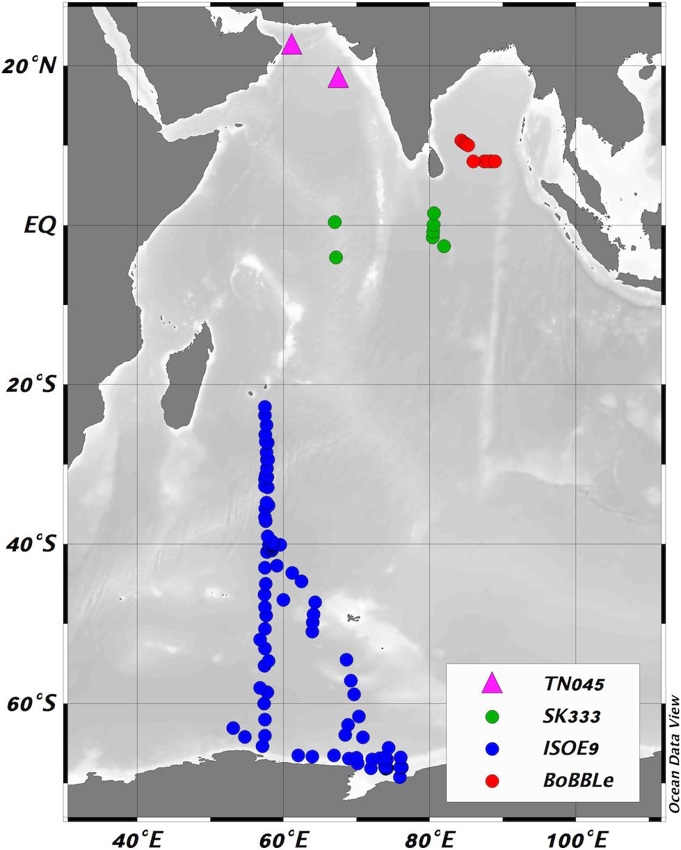
Figure 1. Locations of new sea surface iodide observations made during this work, colored according to cruise (green – SK333, red – BoBBLe, blue – ISOE9) and previous observations from the region made by Farrenkopf and Luther (2002), and included in the compilation of Chance et al. (2014) (pink triangles). Figure produced using Ocean Data View (Schlitzer, 2014).

Materials and Methods

Sample Collection

Samples were collected during three research cruises in the Indian Ocean and Indian sector of the Southern Ocean. Sampling locations for each cruise are shown in Figure 1. Samples were collected from the Bay of Bengal (BoB) during a zonal section cruise (Bay of Bengal Boundary Layer Experiment - BoBBLe) along 8°N, from 85.3°E to 89°E. The cruise took place between 24/6/2016 and 23/7/2016, on board the RV Sindhu Sadhana. In the Arabian Sea, samples were collected during the Rama mooring equatorial cruise IO1-16-SK (known as SK333 here), operated by Ministry of Earth Sciences, India (MoES) and National Oceanic and Atmospheric Administration, USA (NOAA), and taking place on the ORV Sagar Kanya. The cruise departed Chennai, India, on 23/08/2016 and returned to Sri Lanka on 23/09/2016. Samples were collected from the Southern Indian Ocean and Southern Ocean during the 9th Indian Southern Ocean Expedition (SOE9; Jan-March 2017), from Mauritius (22°S) to coastal waters of Prydz Bay, Antarctica (69°S) on board the MV SA Agulhas. Sampling included both (Antarctic) coastal and open ocean waters during this cruise.

During the BoBBLe and SOE9 cruises, surface water samples were obtained manually from the upper 30–70 cm of the sea surface using a metal bucket deployed over the windward side of the ship near the stern. Additional depth profile samples were obtained using a CTD (911 plus, Sea-Bird Electronics, United States) rosette equipped with 12 Niskin bottles. During the SOE9 cruise, depth profiles were taken at 17 CTD stations, and additional surface samples were taken (by bucket) at least twice a day along the entire cruise track (except when the ship was stationary for CTD stations). Sampling included two time-series, one at ∼40°S, and one in coastal Antarctic waters at ∼68°S (around the Polar Front), during which samples were collected at 4 or 6 h intervals for up to 72 h. During the SK333 cruise, samples were only collected using a CTD rosette. Sample dates, times and locations for all cruises are given in the online dataset available from the British Oceanographic Data Centre¹. In this manuscript, both shallow CTD samples (depth ≤ 10 m) and “bucket” samples will be considered to be comparable, and representative of the ocean surface. This follows the approach taken in previous examinations of sea surface iodide concentrations (Chance et al., 2014). Note only surface samples are considered in this manuscript, although selected depth profiles are presented in the Supplementary Material to aid interpretation of surface concentrations.

Immediately following collection, samples were filtered (Whatman GF/F) under gentle vacuum, and transferred to 50 mL polypropylene screw cap tubes. Duplicate aliquots were prepared for each sample. Aliquots were either stored at 4°C for on-board iodide determination within 24 h, or frozen at −20°C for transport back to our laboratories for analysis. The majority (91%) of frozen samples were analyzed within 12 months of collection, and all analyses were complete within 17 months of collection. Inorganic iodine speciation is preserved in frozen samples (≤−16°C) for at least one year (Campos, 1997). Repeat analyses of high and low concentration samples indicated that iodine speciation was preserved during the storage period. To avoid possible contamination, sample bottles for the iodine samples were kept strictly separated from the dissolved oxygen reagents containing iodine.

Iodide and Iodate Analysis

Iodide was determined by cathodic stripping square wave voltammetry (Luther et al., 1988; Campos, 1997) using a μAutolab III potentiostat connected to a 665VA stand (Metrohm) with a hanging mercury drop electrode, an Ag/AgCl reference electrode and a carbon or platinum auxiliary electrode. 12 (or 15) mL of the sample was introduced to a glass cell and 90 (or 112) μL of Triton X-100 (0.2%) was added. The sample was purged with N₂ (oxygen free grade) for 5 min before each measurement. The deposition potential was set at 0 V and deposition times were typically 60 s; scans ranged from 0 to −0.7 V, with a step of 2 mV, a 75 Hz frequency and a 0.02 V wave amplitude. Each scan was repeated 5–6 times, with scan repeatability equal or better than 5%. Calibration was by 2 or 3 standard additions of a KI solution (∼10^–5 or 10^–6 M). Precision was estimated by repeat analysis (n = 6) of selected seawater samples over period of 10 days and was found to be lower than 7% relative standard deviation.

Iodate was measured using a spectrophotometer (UV-1800, Shimadzu; 4 decimal places) after reduction to iodonium (I₃^–) (Truesdale and Spencer, 1974; Jickells et al., 1988). 2.3 mL of the sample was introduced in the 1 cm UV quartz cell, 50 uL of sulfamic acid (1.5 M) was added, and the first absorbance value was obtained after 1 min. Then 150 μL of KI (0.6 M) was added and the second absorbance read after 2.5 min. Iodate concentrations were calculated from the difference between the two absorbances. Calibration was performed daily using a series of KIO₃ standard solutions. Samples were measured at least in triplicate with repeatability better than 5%; reported values are means. Reported errors are calculated by propagation of the standard deviation on the repeated measurements, the errors on the fit of the calibration and error on the volumes pipetted. Note that strictly, this method measures all inorganic iodine in oxidation states from 0 to +5, but as this fraction is dominated by iodate it is taken as a measure of iodate.

Supporting Measurements

Samples from CTD stations use the temperature, salinity and depth data directly obtained from the CTD. Precision of these measurements was as follows: temperature: ±0.001°C; conductivity: ±0.0001 S m^–1; depth: ±0.005% of the full scale. CTD salinity was calibrated using a high-precision salinometer (Guildline AUTOSAL). Temperature and salinity of manually collected “bucket” samples were determined using an outboard thermometer, and the salinometer, respectively.

Samples for nitrate (NO₃^–) analysis were collected in 250 mL narrow mouth polypropylene amber bottles (Nalgene). Each bottle was rinsed twice with the sample water prior to collection. Analysis was performed onboard as soon as possible after sample collection, using an SKALAR SAN+ segmented continuous flow AutoAnalyzer. Precision and accuracy of NO₃^– measurements were ±0.06 and ±0.07 μM, respectively.

Ocean Modeling

The ocean iodine cycling model described in Wadley et al. (2020) was used to evaluate which physical and biogeochemical processes drive the observed trends in iodide concentration in the Indian Ocean and Indian sector of the Southern Ocean. The model comprises a biogeochemical model of iodine cycling embedded in a three-dimensional global ocean circulation framework, and has been calibrated using the data from a recently available extended global sea surface iodide compilation (Chance et al., 2019) which includes the current data set, plus additional depth resolved iodide measurements [see (Wadley et al., 2020) for details]. In the model, iodide production is driven by primary production, and iodide loss (by oxidation) is linked to biological nitrification. A spatially variable I:C ratio is used to allow the model to better capture the observed iodide concentrations.

Results and Discussion

Overview – Global Scale Trends

In total, 127 sea surface iodide observations and 130 sea surface iodate observations were made during the three cruises, including two time series. Measurements were made at 98 different sampling locations, spanning latitudes from ∼12°N to ∼70°S. This is a substantial increase in data coverage for the Indian Ocean and the Indian sector of the Southern Ocean region, which was previously particularly lacking in observations of sea surface iodine speciation (Chance et al., 2014). As noted in the introduction, only two sea surface iodide observations for the Indian Ocean were included in Chance et al. (2014), and both were from the Arabian Sea (see Figure 1).

The lowest iodide concentrations were observed at high latitudes, while the highest concentrations were encountered at the northern extent of the southern sub-tropical region and within the tropics (Figure 2). This latitudinal trend in sea surface iodide concentration broadly follows those observed in other ocean basins (Figure 3). In addition, a “dip” in sea surface iodide concentrations is seen around the equator and elevated concentrations are seen in coastal polar waters, as observed elsewhere (Figures 2, 3; Chance et al., 2010, 2014). While these global scale trends are well documented in the Atlantic and Pacific basins e.g., (Tsunogai and Henmi, 1971; Campos et al., 1999; Truesdale et al., 2000; Bluhm et al., 2011), to the best of our knowledge this is the first time they have been confirmed in the Indian Ocean and the Indian section of the Southern Ocean.

FIGURE 2

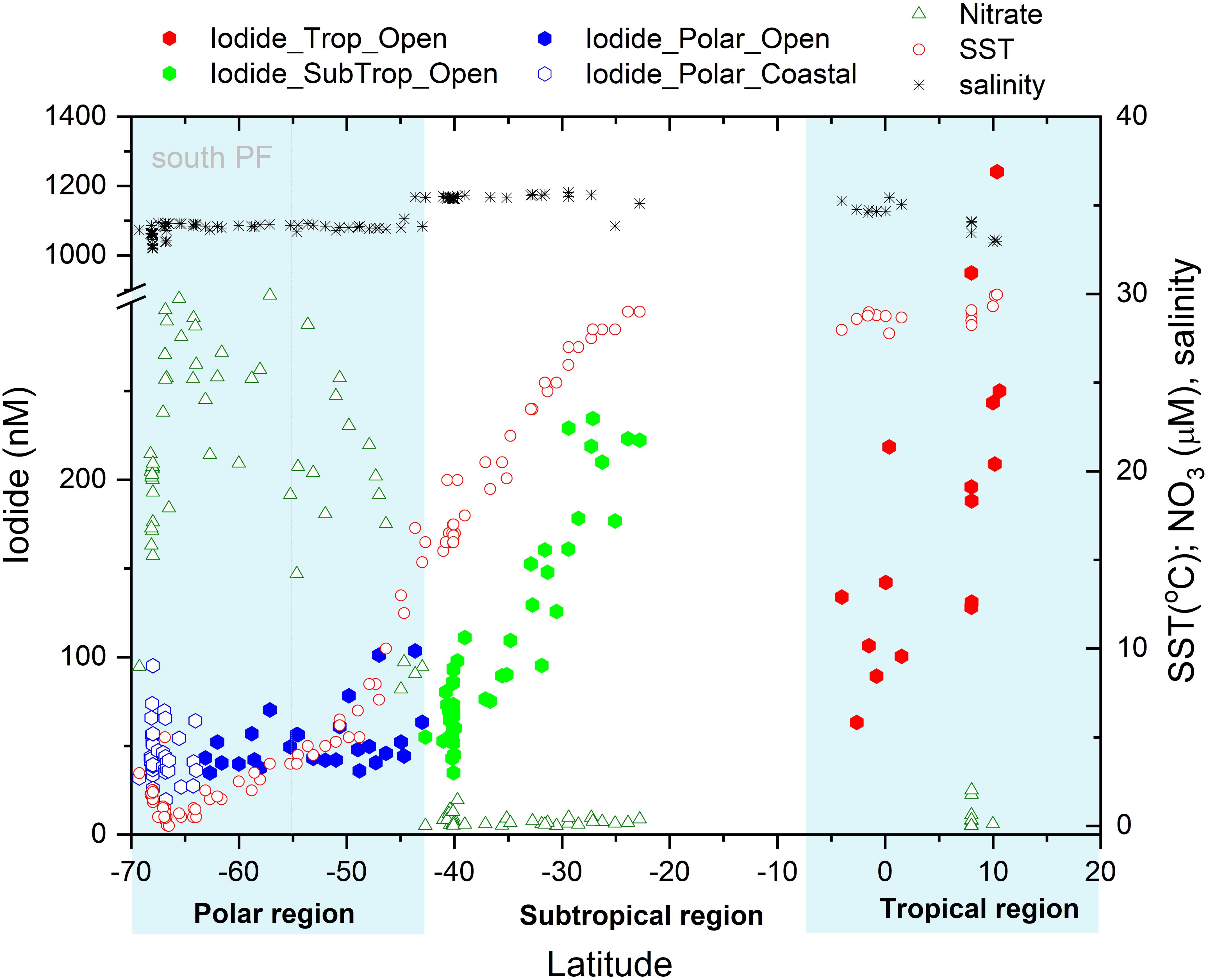
Figure 2. Latitudinal variation of surface iodide concentrations in nM observed in the open Indian and Southern Ocean (●) and in the coastal Southern Ocean (○) compared to the observed sea surface temperature (°C), salinity and nitrate concentrations (μM). Boxes indicate the three different oceanographic regimes considered in the text. The dotted gray line indicates the position of the Polar Front (PF).

FIGURE 3

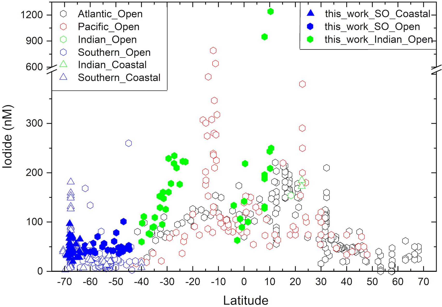
Figure 3. Latitudinal variation of sea surface iodide concentrations in the Indian (green) and Indian sector of the Southern Ocean (SO; blue), compared to other ocean basins (Atlantic – black, Pacific – red). New observations made as part of this work are shown with filled symbols, while other values [see compilation of Chance et al. (2019)] are shown in hollow symbols. Division between ocean basins follows the borders proposed by the World Ocean Circulation Experiment (https://www.nodc.noaa.gov/woce/woce_v3/wocedata_1/woce-uot/summary/bound.htm), and (Orsi et al., 1995) for the Southern Ocean.

Considering the entire data set, sea surface iodide concentrations ranged from 20 to 1241 nM, with a median of 61 nM (Figure 4). The very large range in the data is primarily due to the presence of two very high outliers in the Bay of Bengal, which are discussed later. When these outliers are excluded, the upper limit of the data is reduced to 250 nM, bringing the range within the global range of marine iodide concentrations previously reported (Chance et al., 2014). The large range in the overall data set can mainly be ascribed to the large span of latitudes covered. The median value is somewhat lower than the global median value 77 nM; (Chance et al., 2014), reflecting the bias toward high latitude/low iodide samples in our data set.

FIGURE 4

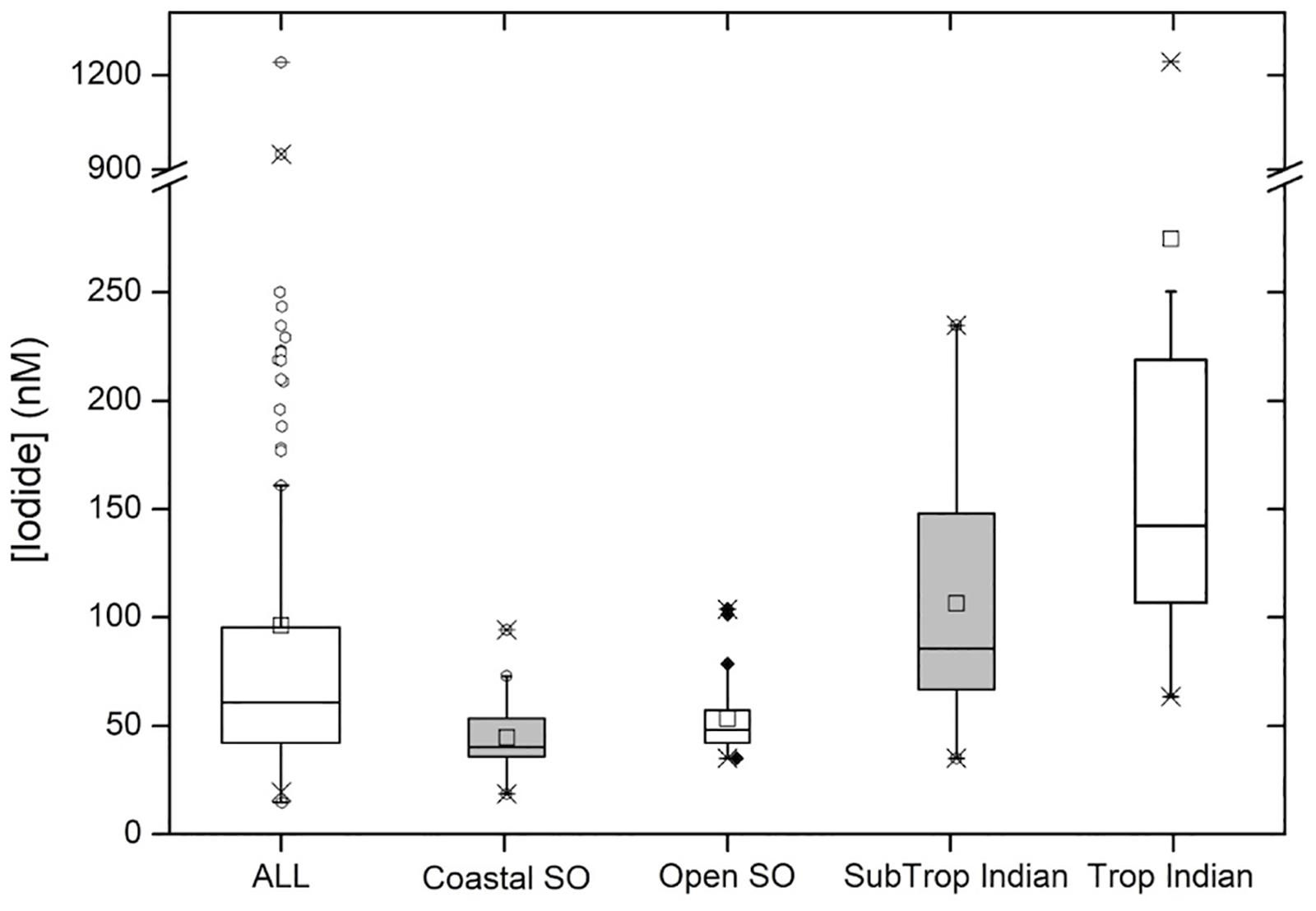
Figure 4. Box and Whisker plot showing descriptive statistics for the entire data set (“ALL”; n = 127) and sub-divided into the following regions: polar coastal waters (“Coastal SO”; n = 38), open waters of the Southern Ocean (“Open SO”; n = 27), the Indian Ocean subtropical convergence zone and southern subtropical gyre (“SubTrop Indian”; n = 46 and the tropical Indian Ocean (“Trop Indian”; n = 16). See main text for more detailed descriptions of these categories. Center lines show the medians; squares are the means; box limits indicate the 25th and 75th percentiles; whiskers extend 1.5 times the interquartile range from the 25th and 75th percentiles, outliers are represented by dots; crosses represent 1st and 99th percentiles; width of the boxes is proportional to the square root of the sample size.

Sea surface iodate concentrations ranged from 51 to 495 nM, with a median of 294 nM. Iodate concentrations broadly showed the opposite pattern to iodide concentrations, with highest median values in the Southern Ocean (median of 323 nM), intermediate values in the subtropical Indian Ocean (median of 294 nM) and lowest values in the tropical Indian Ocean (median 196 nM). However, there was only a very weak, inverse linear relationship between sea surface iodide and iodate concentrations (R² = 0.16, p = 3 × 10^–6; Figure 5). Total iodine concentrations in seawater are typically ∼450–500 nM (Chance et al., 2014, and references therein), with the budget dominated by iodide and iodate. Here we find the sum of iodide and iodate was less than this at most sampling locations (Figure 5), with a median value of 380 nM (range 88 to 560 nM). Although somewhat unusual, comparable low total inorganic iodine concentrations have been reported elsewhere [e.g., North Sea (Hou et al., 2007), South East China Sea (Wong and Zhang, 2003)]. Depleted total inorganic iodine may be due to uptake of iodine to the particulate phase in the surface ocean, or the presence of a significant dissolved organic iodine reservoir. Although it could imply substantial loss of iodine from the surface ocean to the atmosphere, current knowledge suggests the magnitude of such fluxes (e.g., Carpenter et al., 2013) is too small to have such a large impact on the sea surface concentrations. No clear relationships were evident between total inorganic iodine and either latitude or nitrate concentration.

FIGURE 5

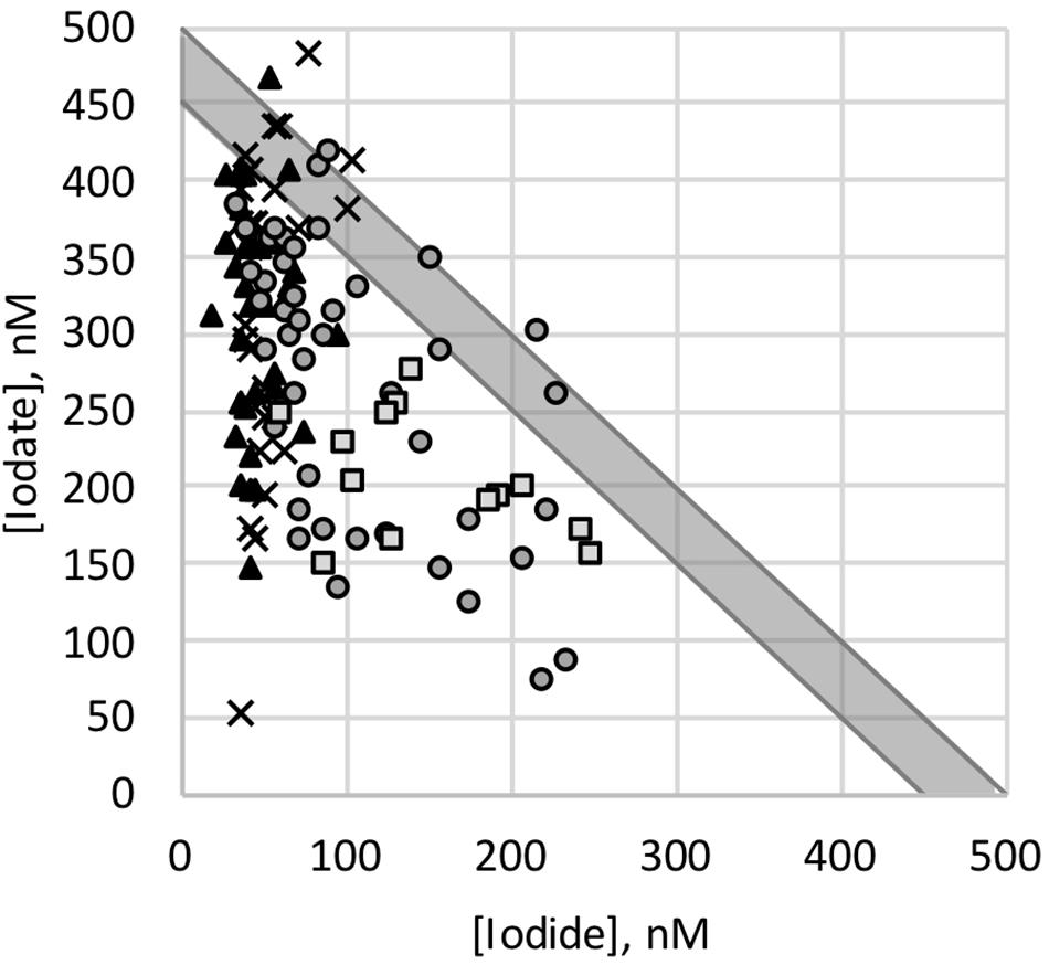
Figure 5. Sea surface iodate concentrations plotted against iodide concentrations, for samples from polar coastal waters (▲), open waters of the Southern Ocean (×), the Indian Ocean subtropical convergence zone and southern subtropical gyre (○) and the tropical Indian Ocean (□). Gray line shows 1:1 relationship, assuming a total inorganic iodine concentration of 450 to 500 nM (Chance et al., 2014). Note for clarity two samples with very high iodide concentrations not shown.

Our sampling area spanned a wide range of different hydrographic provinces and biogeochemical conditions (Figure 2). North of the equator, SST becomes a poor predictor of iodide concentration. To explore our data set further, we consider iodine speciation separately in each of three different hydrographic regimes (tropical, mid-latitudes, and polar).

South Indian Subtropical Gyre (∼23–42°S)

In the southern Indian Ocean, samples were collected along an approximate latitudinal transect at 57°E, from ∼23 to 42°S. The open ocean transect spanned the Indian South subtropical gyre and the subtropical convergence zone. North of this region, at ∼15°S, the Southern Equatorial Current (SEC; not sampled in this work) has been noted as a clear biogeochemical front, separating subtropical gyre waters from the lower oxygen northern Indian Ocean (Grand et al., 2015). The subtropical gyre waters are characterized by very low nitrate concentrations and relatively high salinity (Figure 2), with SST rising from ∼15°C in the south to ∼29°C in the north. Between these latitudes, iodide concentrations ranged from 35 to 235 nM and increased in step with decreasing latitude and increasing SST (Figure 2). In this region, iodide is strongly correlated with both latitude (R² = 0.86, p = 3 × 10^–20) and SST (R²_adj = 0.89, p = 2 × 10^–22) (Table 1). These are stronger correlations than the global relationships reported in Chance et al., 2014, and also have steeper gradients than found in the Chance et al. (2014) data set (Table 1).

TABLE 1

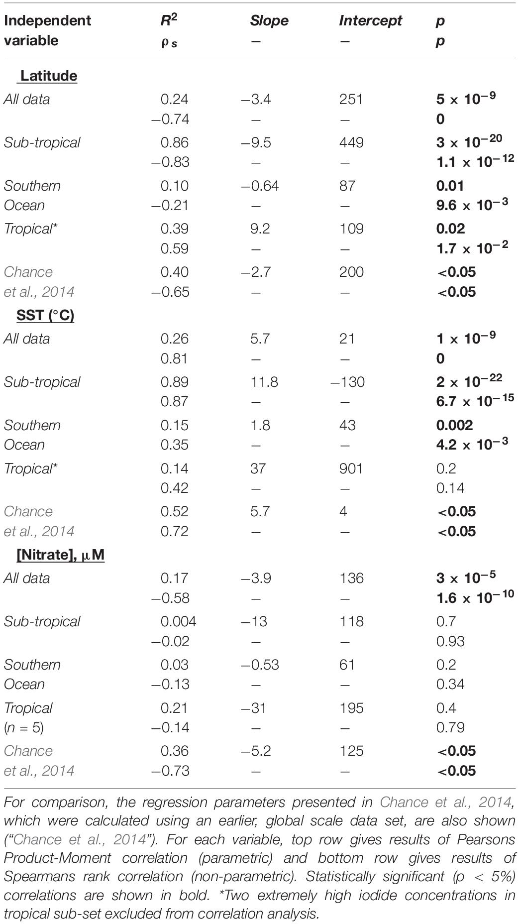
Table 1. Regression parameters for relationships between sea surface iodide (in nM) and latitude, SST and nitrate concentration, for iodide observations made in the Indian Ocean and Indian Ocean sector of the Southern Ocean during this work (“All data”), and hydrographic sub-divisions of this data-set.

Nitrate concentrations have been used to predict sea-surface iodide concentrations (Ganzeveld et al., 2009), and significant relationships between iodide and nitrate in upper 100 m of the water column have been reported for the subtropical Atlantic (Campos et al., 1999). However, in our data set no relationship between nitrate and iodide was apparent (R² = 0.0004; Table 1), implying sea surface nitrate concentrations are a poor predictor of sea surface iodide in this hydrographic region. This likely reflects the fact we only consider surface concentrations, which exhibited low nitrate concentrations (86% of data points were below 0.5 μM), but substantial gradients for iodide.

Comparison of Latitudinal Sea Surface Iodide Gradients Between Subtropical Regions of Different Ocean Basins

Using the extended dataset of global sea surface iodide observations (Chance et al., 2019), sea surface iodide gradients in the subtropical regions of each of the ocean basins were compared (Table 2). Considering each of the major ocean gyres individually reveals that the latitudinal dependency of iodide is greater in the Indian Ocean than in the north Atlantic, north Pacific or south Atlantic (Figure 3 and Table 2). Iodide in the south Pacific appears to also have a steep gradient if observations from the Peruvian upwelling region (Cutter et al., 2018) are included in the analysis. However, this dataset has an unusually large iodide concentration range (153 to 790 nM) within a small latitudinal band (∼11 to 16°S), and does not exhibit a latitudinal trend in iodide as observed elsewhere. This distinct behavior may be due to the influence of sub-surface low oxygen waters. The remaining data from the south Pacific subtropical gyre is from a transect along the 170°W meridian from 12 to 38°S (Tsunogai and Henmi, 1971). If the Peruvian upwelling data is excluded from the gradient analysis, the remaining data for the south Pacific exhibits a comparable iodide gradient to the other ocean basins. The higher sea surface iodide gradient observed in the subtropical Indian Ocean is driven by concentrations at low latitudes (∼25°S) being approximately double those at comparable latitudes in the other ocean basins, rather than a difference between concentrations at the high latitude limits of the gyres (Figure 3).

TABLE 2

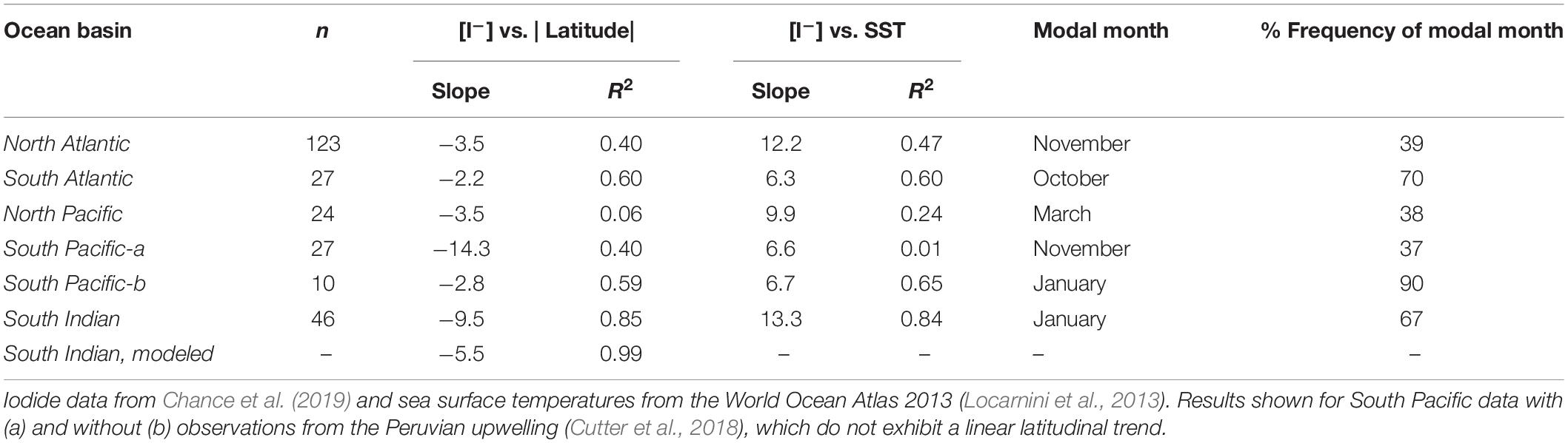
Table 2. Gradients of sea surface iodide concentrations against latitude and sea surface temperature (SST) for open ocean subtropical waters (defined by province) of the global ocean basins.

The same trend is also evident in iodide vs. SST gradients, which are steeper in the Indian Ocean than in other basins (Table 2). This implies that the differences between basins cannot entirely be accounted for by differences in SST gradients. Examination of climatological data (World Ocean Atlas, see Chance et al., 2014 for details) for the locations and months of iodide observations does not demonstrate any clear differences in SST, nitrate or mixed layer depth (MLD; defined using potential temperature) between ocean basins that might account for the difference in iodide gradient. Although SST is not thought to directly impact iodine cycling itself, its correlation with iodide concentration is important as it is widely used to predict sea surface iodide fields for use in atmospheric models (e.g., Sarwar et al., 2016). The stronger latitudinal dependency of iodide in the Indian Ocean that we observe here is not replicated in sea surface iodide values predicted using commonly employed global scale parameterizations based on sea surface temperature (Chance et al., 2014; MacDonald et al., 2014). This is likely to introduce uncertainties specific to the Indian Ocean when using such parameterizations, for example in model calculations of iodine emissions from the sea surface.

The observational data is too limited to properly evaluate whether the pattern is the result of seasonal biases in sampling; of the data used in this comparison, all subtropical Indian Ocean observations were made during the southern hemisphere summer (January and February), while the modal months for observations in other basins were November (North Atlantic), October (South Atlantic) and March (North Pacific), see Table 2. In the South Pacific, if data from the Peruvian upwelling is excluded, at least 90% of observations used were made in January (Tsunogai and Henmi, 1971), i.e., in the same season as the Indian Ocean data. Despite this, they have a lower latitudinal gradient (slope = 2.8 compared to 9.5; Table 2), hinting that the difference between basins is not due to seasonal variation and/or sampling biases and may instead be due to differences in iodine cycling.

Although less pronounced, a relatively steep iodide vs. latitude gradient in the Indian Ocean is replicated in our model (Table 2), and hence a series of model sensitivity tests have been conducted to investigate which processes may be responsible for the apparent differences in the iodide gradient between ocean basins. Specifically, the model was run with each of the iodide forcing processes in the Indian Ocean and Indian sector of the Southern Ocean replaced by those from the Atlantic. Figure 6 shows the forcing fields used for the two ocean basins, and the modeled iodide concentrations generated using these fields. The iodide vs. latitude gradient is significantly increased between 30°S and 20°S when the Indian Ocean productivity fields are replaced with those for the same latitudes in the Atlantic (Figure 6c). This is driven by a smaller decrease in productivity with decreasing latitude in the Indian Ocean than the Atlantic (Figure 6b). Thus productivity differences would act to decrease, rather than increase the iodide gradient. In the model oxidation of iodide in the mixed layer occurs as a function of nitrification, which is parameterized using the proportion of nitrate regenerated in the mixed layer (see Wadley et al., 2020). Differences in this ratio between the subtropical regions of the Indian and Atlantic oceans are small (Figure 6d), and have negligible impact on modeled iodide in the Indian Ocean (Figure 6e). At lower latitudes MLDs are similar in the two basins, but between ∼35 and 45°S, MLDs are significantly deeper in the Atlantic due to the greater northward extent of polar waters (Figure 6f). Since a deeper MLD dilutes iodide, modeled iodide concentrations are decreased between 45°S and 35°S when Atlantic MLDs are imposed in the Indian basin (Figure 6g). Again this further increases the latitudinal gradient of iodide, rather than decreasing it. Precipitation and evaporation act to dilute/concentrate iodide in the mixed layer, so changes in the net freshwater flux with latitude could influence the latitudinal iodide gradient. However, imposing the Atlantic surface freshwater flux in the Indian Basin had a negligible effect on modeled iodide (Figure 6i). Finally, the I:C ratio in the model determines the amount of iodide produced per unit carbon fixed by primary production. To fit model to the observed iodide in each basin, a higher I:C ratio is utilized in the Indian than in the Atlantic Ocean (Figure 6j; see Wadley et al., 2020). Replacing the I:C ratio in the Indian Ocean with that for the Atlantic Ocean results in lower modeled iodide concentrations in the Indian Ocean, but little overall change in the latitudinal iodide gradient (Figure 6k). Note the model currently underestimates the iodide gradient in the Indian Ocean (Table 2), and further refinement of the spatial variation in the I:C ratio is needed to improve the model fit to observations. This may show that the I:C ratio influences latitudinal gradients of iodide.

FIGURE 6

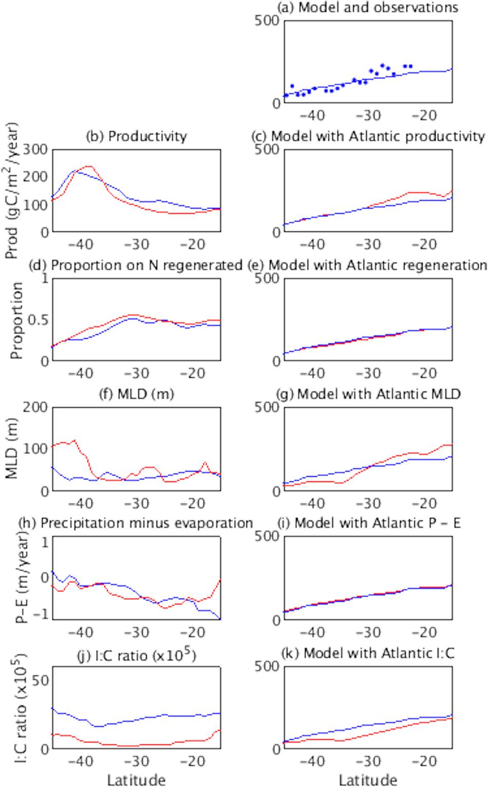
Figure 6. Impact of imposing Atlantic forcings in the Indian Ocean basin in the iodine cycling model. Plots are annual mean iodide for 57°E in the Indian Ocean. (a) observed (dots) and modeled (line) iodide, in nM (b,d,f,h,j) latitudinal sections for each process-related quantity for the Indian (blue) and Atlantic (red) Oceans, (c,e,g,i,k) corresponding latitudinal sections of iodide for control (blue) and Atlantic forcing imposed over the Indian basin (red).

In summary, basin scale differences in four key forcing fields (productivity, nitrification, MLD and P-E) do not appear to explain the difference in latitudinal iodide gradient between the subtropical Indian and southern Atlantic oceans. In fact, differences in productivity and MLD between the two basins appear to have the opposite effect, as Atlantic forcing fields resulting in an even steeper gradient than Indian Ocean forcing fields. Removal of advection in the model also results in an increase rather than a decrease in iodide at sub-tropical latitudes in the Indian Ocean (see later/Figure 7) and hence an even steeper latitudinal iodide gradient. This suggests the basin scale differences in iodide gradient are not due to advection in the Indian Ocean. Instead we suggest the difference may be the result of different phytoplankton types, with differing I:C iodide production ratios between basins. The need for a higher I:C ratio in the Indian Ocean/Indian sector of the Southern Ocean than the Atlantic (Figure 6j) implies there may be profound differences in microbiological community composition, and/or the cycling of iodine by such organisms between basins. Synechococcus dominates in the subtropical Indian Ocean, whereas Nanoeucaryotes and Prochlorococcus dominate in the subtropical Atlantic (Alvain et al., 2008). Recent work by our group indicates that the I:C ratio associated with iodide production varies between phytoplankton types, with Synechococcus having a higher I:C ratio than Nanoeucaryotes and Prochlorococcus types (Wadley et al., Manuscript in Preparation). Hence the higher relative abundance of Synechococcus in the subtropical Indian Ocean might account for the higher iodide concentrations observed at low latitudes, and the resulting steeper sea-surface iodide gradient. This also indicates that any change in microbiological community composition associated with climate change could significantly impact ocean iodide concentrations.

FIGURE 7

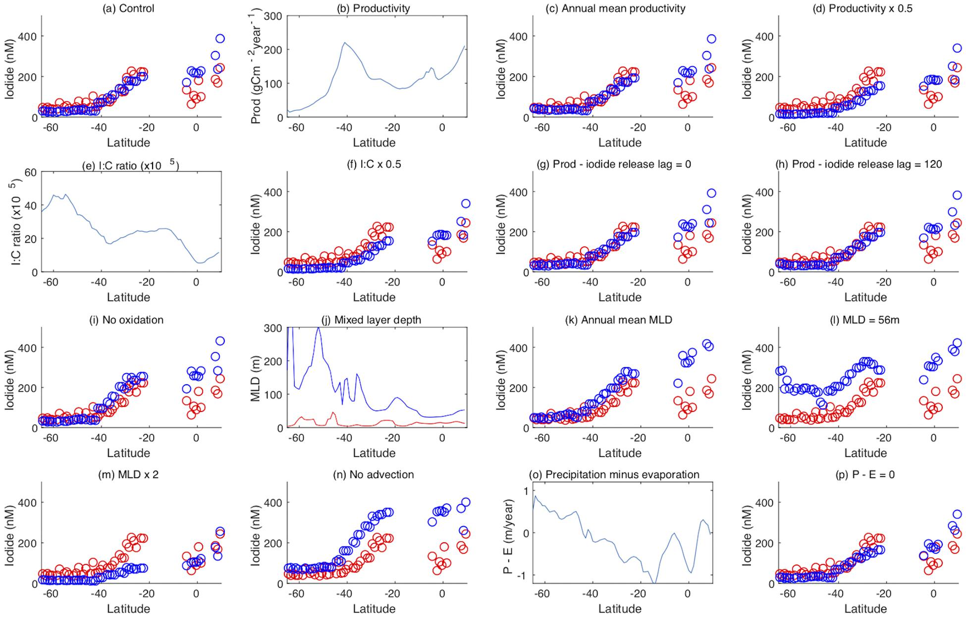
Figure 7. Results from model process sensitivity experiments. (a) Observed (red) and model (blue) iodide concentrations as a function of latitude, in the Indian Ocean and the Indian sector of the Southern Ocean along a section at 60°E (note observed iodide over 500 nM have been excluded here) (b) observed primary productivity (Behrenfeld and Falkowski, 1997) as a function of latitude, (c) iodide with the seasonal cycle of productivity replaced with the annual mean, (d) iodide with seasonal productivity halved, (e) the model I:C ratio, (f) iodide with the model I:C ratio halved, (g) iodide with iodide release from plankton at the same time as carbon assimilation, (h) iodide with iodide release from plankton lagged 120 days from carbon assimilation, (i) no mixed layer oxidation of iodide, (j) maximum (blue) and minimum (red) mixed layer depth from the OCCAM model (Aksenov et al., 2010) as a function of latitude, (k) iodide with the seasonal cycle of mixed layer depth replaced with the annual mean, (l) iodide with the seasonal cycle of mixed layer depth replaced by the constant global mean of 56 m, (m) seasonal MLD doubled, (n) no vertical or horizontal advection, (o) P-E from the OCCAM model (Aksenov et al., 2010) as a function of latitude, (p) P-E set to zero.

Southern Ocean Domain (∼42°S–68°S)

At the subtropical front around 42°S, a decrease in salinity is accompanied by a sharp increase in nitrate concentration (Figure 2). This front marks the transition from the Indian Ocean to the Southern Ocean (Orsi et al., 1995). The colder, nutrient rich waters south of the subtropical front have much lower iodide content, with a median concentration of 43 nM and range of 20–104 nM (Figure 4). Relationships between iodide concentrations and latitude or SST in this region are much weaker than those observed further north (Table 1). This may be due to disruption by strong, but variable, vertical mixing events, which are characteristic of the Southern Ocean. No significant relationship between sea surface iodide and nitrate was observed in the Southern Ocean samples (Table 1).

The Southern Ocean samples may be further subdivided into coastal (i.e., near the Antarctic continent) and open ocean samples. The former category was defined as samples falling within the Austral Polar biogeochemical province (Longhurst, 1998), while the latter category included samples from both the Antarctic and Sub-Antarctic provinces, and spanned the Polar Front. The range and distribution of concentrations seen in the coastal and open ocean subsets are very similar (Figure 4), despite the coastal samples spanning a much narrower latitudinal range (69–64°S, compared to 63–43°S). In the open ocean sub-set, iodide concentrations generally decrease moving south (R² = 0.16; p = 0.04), while in the coastal samples at the most southerly extreme of the data set, this relationship breaks down (R² = 0.02; Figure 2). A similar pattern is also reported in the global compilation of Chance et al. (2014), where Southern Ocean and Antarctic samples were predominantly from the Atlantic sector and the western Antarctic Peninsula. The range of concentrations observed in the Antarctic coastal samples (20 to 95 nM) is within that observed previously in coastal Antarctic waters during the austral summer (Chance et al., 2010). The magnitude of this variability is greater than can be accounted for by normalizing the iodide concentrations to salinity variations (e.g., due to ice melt water).

Northern Indian Ocean Including Southern Bay of Bengal (∼4°S–11°N)

Samples were collected from open ocean locations in the Bay of Bengal and the Arabian Sea, between ∼4°S and ∼11°N. Sampling locations were all within the Indian Monsoon Gyre biogeochemical province (Longhurst, 1998), and shared high sea-surface temperatures, variable salinity and typically low nitrate concentrations. This sample sub-set showed the highest, and most variable iodide concentrations (range 63–1241 nM, median 165 nM; Figure 4). This was primarily due to the occurrence of two extremely high iodide concentrations (>900 nM) in the Bay of Bengal; excluding these values, the range in tropical open ocean iodide was still the largest of the three hydrographic regions surveyed, with a maximum of 250 nM being observed in the Bay of Bengal (Figure 4). Such concentrations are comparable to measurements made at similar latitudes elsewhere (Figure 3).

All but one of the samples collected around the equator (∼5°S to ∼3°N) during the SK333 cruise had iodide concentrations in the range ∼80 to 120 nM. The exception to this was a station at 0°N where iodide concentrations reached ∼200 nM (Figure 2). As iodide concentrations were typically lower than in tropical waters further north and south (Figure 2), there was a positive rather than negative correlation between iodide and absolute latitude in this sample set (Table 1). A similar dip at very low latitudes is also seen in the Atlantic and Pacific (Figure 3; Chance et al., 2014). This feature is replicated in our model and is thought to be due to the advection and vertical mixing associated with the seasonally varying equatorial current system (see section).

As already noted, exceptionally high sea surface iodide concentrations of 1241 and 949 nM were observed at two stations in the Bay of Bengal (BS3 and BS8). Very high near-surface iodide concentrations were also observed at Station AR nearby (2039, 1546, and 479 nM at 10, 25, and 50 m, respectively, see Supplementary Figure S1). We believe these concentrations are real, and not the result of contamination or analytical error because: (i) repeat analyses gave the same results, (ii) very high concentration samples were also analyzed by ion chromatography, a completely independent method, and this yielded concentrations within 10% of those obtained by voltammetry (1277 and 960 nM for samples BS3 and BS8, respectively, and 1693 nM for Station AR at 25 m depth), (iii) results for Station AR show oceanographic consistency (see Supplementary Figure S1), (iv) no likely sources of iodine contamination were present during sampling. It is possible that the high, very localized, iodide concentrations could arise from the break-down of an iodine rich substrate, for instance a mass of brown macroalgae such as Laminaria digitata. However, nothing unusual of this nature was observed during sampling. These very high iodide levels result in total (dissolved) inorganic iodine concentrations more than double (2.2 and 2.6 times larger) the near universally observed value of ∼450–500 nM (Chance et al., 2014). This amount of iodide cannot be accounted for solely by the reduction of iodate in the water column (as this could only yield concentrations up to ∼500 nM). Instead it implies an exogenous source of iodine, which is either already in the form of iodide, or is reduced to iodide following introduction to the water column.

Samples with elevated iodide exhibited relatively low surface salinity (Supplementary Figure S1), possibly indicating an association with freshwater inputs. The Bay of Bengal is characterized by very heterogenous salinity - low salinity is caused by monsoon rainfall and high riverine inputs to the north, while high salinity water arrives from the Arabian Sea via the intense Southwest Monsoon Current (SMC). The BoBBLe cruise took place during the Asian summer monsoon season, during which the region experiences high rainfall. However, atmospheric wet deposition is thought unlikely to be the source of elevated iodide because meteoric water has a lower iodine content than seawater [20–124 nM (Sadasivan and Anand, 1979); 4.7–26.2 nM; (Gilfedder et al., 2007)]. Furthermore, observations of elevated sea surface iodide did not correspond to rainfall events encountered during the BoBBLe cruise itself. Similarly, riverine inputs are unlikely to be the iodide source, as total iodine concentrations in rivers, including the Ganges, are lower than or comparable to those in seawater [≤20 ug/L, ∼ 157 nM; (Moran et al., 2002; Ghose et al., 2003)], and the area surveyed was away from major outflows. While freshwater inputs are thus not thought to be the source of the excess iodide, stratification caused by rainwater dilution of surface layers could plausibly contribute to the persistence of high iodide concentrations at the ocean surface.

In addition to the SMC, the second main oceanographic feature in the BoBBLe study area is a wind driven upwelling feature called the Sri Lanka Dome (SLD), which manifests as a large cyclonic gyre in the south western part of the BoB to the east of Sri Lanka. Both the SLD and the SMC were well developed and distinct during the study period (Vinayachandran et al., 2018). Extreme iodide values were observed at stations north (AR, BS3) and east (BS8) of the SLD, but not in the stations that were inside the SLD (Supplementary Figures S1, S2; Vinayachandran et al., 2018). High iodide station AR exhibited high seawater pCO₂ (467–554 atm), low surface pH and low alkalinity, indicative of upwelled waters that are presumed to be associated with the SMC (Vinayachandran et al., 2018). Station BS3 was close in space and time, while station BS8 was also influenced by the SMC (Vinayachandran et al., 2018). We therefore speculate that the high iodide observed is in some way related to the SMC. However, the high salinity core of the SMC (i.e., Arabian Sea water), which was evident at depths of ∼25–150 m at stations east of the SLD, was not itself associated with elevated iodide (Supplementary Figure S1). This suggests the excess iodide was not in the main water mass carried by the SMC, and did not originate from the Arabian Sea. Instead we suggest its source could be coastal waters that are entrained in the periphery of the SMC and carried into the BoB with it.

Comparable high iodide concentrations have previously been observed in low oxygen sub-surface waters in the north western part of the Arabian Sea (Farrenkopf and Luther, 2002); these were attributed to advection from shelf sediments. More recently, plumes of very high iodide sub-surface concentrations (∼1000 nM) have also been reported in sub-oxic waters in the Eastern Tropical South Pacific (ETSP) (Cutter et al., 2018) and the Eastern Tropical North Pacific (ETNP) (Moriyasu et al., 2020). In both cases some outcropping of elevated iodide concentrations at the ocean surface was observed (Cutter et al., 2018; Moriyasu et al., 2020). In the ETSP, the plume followed an isopycnal and was associated with corresponding features in Fe(II) and nitrite, so was again thought to be due to a shelf sediment iodide source (Cutter et al., 2018). Elevated concentrations persisted more than 1000 km from the shelf break due to the relatively long iodide lifetime in seawater with respect to oxidation. Trace metal concentrations were not measured during the BoBBLe cruise, but sub-surface waters in the region have previously been reported to contain additional dissolved Fe from sedimentary inputs (Grand et al., 2015), suggesting it is plausible that stations on the edge of the SLD could be influenced by sedimentary interactions. Waters over the western Indian shelf experience severe hypoxia (Naqvi et al., 2000), and so could be subject to significant sedimentary iodide inputs as implicated in other low oxygen regions (Farrenkopf and Luther, 2002; Cutter et al., 2018). During the Southwest Monsoon, the West Indian Coastal Current flows south along the west coast of India, and these waters are advected along the path of the SMC into the BoB. We speculate that such waters have potential to contain “excess” iodide levels as a result of sedimentary inputs, and that it is the remnants of these water masses that we may have sampled. Iodide has a long lifetime in oxygenated seawater (6 months to several years; Chance et al., 2014; Hardisty et al., 2020), and so a signal may be expected to persist where other indicators of sedimentary inputs are lost (Cutter et al., 2018), and could potentially reach the ocean surface via upwelling areas such as the south western BoB (Supplementary Figure S2).

In the northern Indian Ocean agreement between model and observations is poorer than elsewhere, but modeled concentrations fall within the range of the observations in the area. Furthermore, the model predicts unusually high iodide concentrations in the BoB, where extremely high iodide concentrations were observed. As the model does not currently include sedimentary processes, this suggests additional physical and biogeochemical processes may also contribute to elevated iodide levels in the BoB.

We believe this is the third reported observation of very elevated (>500 nM) iodide concentrations at the surface of the open ocean. The dataset reported by Cutter et al. (2018) contains two surface samples with iodide concentrations of 594 and 960 nM immediately off the coast of Peru, while transects in Moriyasu et al. (2020), show patches of high iodide outcropping at the surface. An extreme surface iodide concentration of ∼700 nM has also been reported for the brackish waters of the Skaggerrak (Truesdale et al., 2003), a shallow strait that is subject to hypoxia (Johannessen and Dahl, 1996). The paucity of previous observations suggests it is a rare phenomenon, but it may nonetheless be of local significance.

Atmospheric ozone deposition and iodine emission fluxes will proportionally increase where surface iodide concentrations are high. An increase in iodide from 150 to 2050 nM (×13.7) leads to a 5–6-fold increase in total iodine emissions, for a typical ambient ozone concentration of 25 ppb and a wind speed of 7 m s^–1 (Supplementary Figure S3). This comprises a 4.5-fold increase in HOI emissions, which dominates the flux, and a 30-fold increase in I₂ emissions, which increase from 5.5% of the total flux at 150 nM iodide to 28% at 2050 nM iodide. It is assumed that the regional atmospheric impact of such “hot-spots” will be low, as they will only represent a small proportion of the relevant footprint area. However, the atmospheric impacts of such areas may become significant if either very localized processes are being considered, or their extent and/or frequency of occurrence increases. As areas of low oxygen waters in contact with shelf sediments become more extensive (Naqvi et al., 2000), the possibility that this could impact on surface iodide concentrations in coastal regions may need to be considered. Understanding the potential impact of low oxygen conditions and sedimentary inputs on surface iodide concentrations, and hence local atmospheric chemistry, requires both the sedimentary fluxes and the lifetime of iodide in oxygenated seawater to be better constrained. The atmospheric boundary layer above the northern Indian Ocean has high iodine oxide (IO) levels, with inputs dominated by the inorganic iodine flux from the ozone-iodide reaction (>90%), as a result of “ozone-related” pollution outflow (Prados-Roman et al., 2015). Hence atmospheric chemistry in the region may be particularly sensitive to changes in the surface iodide budget.

Exploring Physical and Biogeochemical Controls on Sea Surface Iodide in the Indian Ocean Using the Ocean Iodine Cycling Model

The trends in sea surface iodide concentrations observed across the south Indian subtropical gyre and Indian sector of the Southern Ocean are well replicated by the iodine cycling model of Wadley et al. (2020) (Figure 7a). We used the model to explore how physical (MLD, advection, net surface freshwater flux) and biogeochemical (productivity, iodide formation to carbon fixation ratio) factors influence iodine cycling in the study area.

Biological productivity drives iodide formation in the model, but has a different spatial distribution to iodide in the Indian Ocean basin (Figures 7a,b). Although both tend to increase moving north along the transect, the very strong peak in productivity centered on 40°S (Figure 7b) has no corresponding peak in either observed or simulated iodide concentrations. This indicates that other processes are also important in determining the iodide distribution. Imposing a constant level of productivity (set at the annual mean for each grid point) throughout the year had very little effect on modeled iodide concentrations, (Figure 7c), suggesting that the seasonal cycle of iodide production does not have a dominant effect on iodide concentrations. Halving the productivity in the model reduces simulated iodide concentrations by around a half south of 40°S (where iodide is very low, and iodate high), but only by around a quarter north of 40°S, and has almost no effect in the northern Indian Ocean where modeled iodide is highest (and thus modeled iodate lowest, at ≤300 nM). This may indicate that lower iodate concentrations to the north limit iodide production. The amount of iodide produced per unit primary productivity is specified in a spatially variable I:C ratio (Figure 7e; (Wadley et al., 2020). Halving this ratio is equivalent to halving primary production, and has identical consequences (Figure 7f).

As iodide is assumed to be evenly distributed throughout the mixed layer, surface concentrations are dependent on the MLD. Summer MLD minima are similar throughout the section, with typical values of a few tens of meters, whereas late winter MLD maxima increase with latitude (Figure 7j). Deepening of the MLD decreases iodide concentrations throughout the mixed layer as a result of dilution, while shoaling of the MLD decreases the total amount of iodide present integrated over the mixed layer, but does not change the concentration at any given depth within it. Removing the seasonal cycle of MLD in the model (by replacing with the annual mean MLD for each grid point) increases surface iodide concentrations, particularly at lower latitudes (Figure 7k), indicating that the removal of iodide through MLD shoaling is important. Removing both seasonal and spatial variation in the MLD by setting it to a uniform 56 m results in substantial increases in surface iodide concentrations at higher latitudes (Figure 7l), due to elimination of both dilution and shoaling effects. In contrast, doubling the MLD decreases iodide concentrations, with the greatest effect seen where iodide concentrations are highest (Figure 7m). Interestingly, this brings modeled and observed iodide concentrations into good agreement around the equator. Inspection of SK333 CTD data indicates that at the time of sampling, actual MLDs in this region (between 50 and 100 m) were deeper than the climatological values used in the model (less than 40 m; Figure 7j), which may indicate that short term variations in MLD, for example due to weather events, affected iodide concentrations.

In the model, phytoplankton mediated iodide formation occurs 60 days after the uptake of carbon, and the interplay of this lag period with the MLD cycle could influence iodide concentrations. However, changing the duration of the lag to 0 and 120 days in the model has only a small impact on the iodide, and only at high latitudes (Figures 7g,h).

The seasonal MLD cycle imposes an annual timescale on the removal of iodide from the mixed layer where the seasonal cycle has a large amplitude, but vertical and horizontal advection also exchange water between the surface layer and ocean interior. Turning off the circulation in the model, so that vertical mixing is the only physical mechanism for iodide removal from the mixed layer also results in increased mixed layer iodide concentrations at almost all locations (Figure 7n).

In addition to removal by MLD shoaling, the model also allows for the removal of mixed layer iodide by oxidation to iodate, via a pathway linked to nitrification (Wadley et al., 2020; Hughes et al., under review). Eliminating this pathway has little impact on modeled iodide concentrations at high latitudes, but results in a significant increase in concentrations north of 40°S (Figure 7i). This is because the iodide oxidation timescale in the model is multi-annual, and hence its impact is modulated by the lifetime of iodide in the mixed layer with reference to vertical mixing. At high latitudes, large seasonal changes in the MLD result in low sensitivity to oxidation, whereas at lower latitudes there is less annual mixed layer exchange, resulting in a longer iodide residence time, and hence oxidation is a more important process for mixed layer iodide removal.

The net surface freshwater flux resulting from precipitation and evaporation (P-E) acts to, respectively, dilute or concentrate iodide in the mixed layer (Figure 7o). Setting the P-E flux to zero has a small impact on iodide, decreasing concentrations in the subtropical gyres where evaporation is strong. Thus at these latitudes evaporation results in a modest increase in iodide concentrations.

The model sensitivity tests described above confirm that sea surface iodide concentrations in the Indian and Southern Oceans are determined by a combination of factors which interact non-linearly. The dominant processes that determine iodide concentrations are the rate of iodide production, which is a function of productivity and the I:C ratio, and the MLD and its seasonal cycle, which acts to dilute and remove iodide from the surface layer. Loss by oxidation has the greatest impact at lower latitudes where physical removal mechanisms are weakest. As the climate changes over coming decades, changes in any of these factors are likely to result in changes in sea surface iodide concentrations. For example, the 100 to 300 m depth layer in the Indian Ocean has significantly warmed since 2003 as a result of heat distribution from the Pacific (Nieves et al., 2015) and this is likely to reduce stratification, and enhance vertical mixing, with an accompanying reduction in mixed layer iodide concentrations. Conversely, changes in nutrient inputs to the Indian Ocean and declining oxygen levels will act to reduce iodide oxidation, due to its association with nitrification (Hughes et al., under review), and hence may act to increase iodide concentrations. Any changes in productivity, and/or shifts to different phytoplankton types with different I:C ratios, will also potentially alter the rate of iodide production, although this has been found to predominantly impact on iodide concentrations at higher latitudes (Wadley et al., manuscript in preparation).

Concluding Remarks

The 127 sea surface iodide observations examined here represent a substantial (>10%) increase in the number of measurements that have been made across the global oceans (925 individual observations were included in Chance et al., 2014). They span nearly 80 degrees latitude in the Indian Ocean and Indian sector of the Southern Ocean, a region where very few (n = 2) surface observations were previously available. This increase in observations will facilitate better predictions of sea surface iodide concentrations, and consequent atmospheric chemistry, and the data has already been incorporated in a new global iodide database (Chance et al., 2019) and parameterization (Sherwen et al., 2019).

The large scale latitudinal trends observed in the Indian Ocean and Indian sector of the Southern Ocean are similar to those in other ocean basins (Chance et al., 2014). At subtropical latitudes, the latitudinal and temperature dependency of iodide is steeper than in other ocean basins. Therefore, using global scale relationships with SST [e.g., (MacDonald et al., 2014)] to predict regional scale iodide concentrations for the Indian Ocean will be subject to biases. Exploration of this basin scale difference using a state-of-the-art global iodine cycling model (Wadley et al., 2020) indicates that it may be driven by differences in biological iodide production. We have also used the model to explore the controls on the sea-surface iodide distribution in the Indian Ocean basin. Model sensitivity tests indicate that sea surface iodide is likely to be a function of vertical mixing and the seasonal cycle in MLD, the rate of iodide production, which is related to productivity and the I:C ratio, and – at lower latitudes – iodide oxidation in the mixed layer. These factors interact in a non-linear manner.

Exceptionally high iodide concentrations were observed at a small number of stations in the northern Indian Ocean. Such high concentrations are rare, but have been reported previously in low oxygen subsurface waters (Farrenkopf and Luther, 2002), and more recently, in surface waters above the Peruvian and Mexican oxygen deficient zones (Cutter et al., 2018; Moriyasu et al., 2020). In all cases, the excess iodide is suggested to be sedimentary in origin, raising the possibility that processes at the sea floor could influence air-sea interactions, should that water reach the sea surface. Although such iodide “hot-spots” are unlikely to have significant impact on a global or regional scale, it is possible they may impact on local scale air-sea exchange processes involving iodine. Their existence also means care must be taken to ensure iodide concentrations used to generate parameterizations are representative of the entire study area.

Marine iodine cycling is anticipated to be affected by global change, with consequent impacts on atmospheric chemistry. The Indian Ocean basin is subject to a number of specific pressures with potential to affect iodine cycling. Despite the empirical relationship between SSI and SST, changes in vertical mixing as a result of the Indian Ocean warming may in fact reduce mixed layer iodide concentrations. Meanwhile, changes to biological processes as a result of anthropogenic nutrient inputs, ocean deoxygenation and changes in heat distribution are likely to impact iodide production and loss processes. Such changes will in turn impact ozone deposition and iodine emission from the sea surface.

Data Availability Statement

Sea surface iodide concentration data described in this work is available from the British Oceanographic Data Centre, as part of a global compilation of observations 10/czhx (Chance et al., 2019). Additional supporting datasets are available on request to the corresponding author.

Author Contributions

LT, AS, AKS, and AM collected seawater samples during the three research cruises. LT and RoC analyzed the samples for iodine speciation. AS, AKS, and RR provided the supporting biogeochemical measurements. RaC and PS provided insight regarding physical oceanography in the study area. DS and MW performed the iodine modeling described in section “Concluding Remarks.” RoC and LT interpreted the data and wrote the manuscript with input from TJ and MW, other authors also provided comments on the manuscript. LC, TJ, AM, and RoC conceived the study. All authors contributed to the article and approved the submitted version.

Funding

This work was funded by United Kingdom NERC grants NE/N009983/1 and NE/N01054X/1 awarded to RoC, LT, TJ, MW, DS, and LC. The research cruises were funded by the Ministry of Earth Sciences, India, and we thank the National Centre for Polar and Ocean Research for generously providing LT a berth on the SOE-09 expedition.

Conflict of Interest

The authors declare that the research was conducted in the absence of any commercial or financial relationships that could be construed as a potential conflict of interest.

Acknowledgments

We are grateful to the officers, crew and scientific parties onboard MV SA Agulhas, ORV Sagar Kanya, and RV Sindhu Sadhana for their essential support during the research cruises. We also thank Alex R. Baker (University of East Anglia) for loan of analytical equipment, and Matt Pickering (University of York) for help with ion chromatography analysis. The model simulations were undertaken on the High Performance Computing Cluster supported by the Research and Specialist Computing Support service at the University of East Anglia.

Supplementary Material

The Supplementary Material for this article can be found online at: https://www.frontiersin.org/articles/10.3389/fmars.2020.00621/full#supplementary-material

Footnotes

1. ^ http://doi.org/czhx

References

Aksenov, Y., Bacon, S., Coward, A. C., and Nurser, A. J. G. (2010). The North Atlantic inflow to the Arctic Ocean: high-resolution model study. J. Mar. Syst. 79, 1–22. doi: 10.1016/j.jmarsys.2009.05.003

CrossRef Full Text | Google Scholar

Allan, J. D., Williams, P. I., Najera, J., Whitehead, J. D., Flynn, M. J., Taylor, J. W., et al. (2015). Iodine observed in new particle formation events in the Arctic atmosphere during ACCACIA. Atmos. Chem. Phys. 15, 5599–5609. doi: 10.5194/acp-15-5599-2015

CrossRef Full Text | Google Scholar

Alvain, S., Moulin, C., Dandonneau, Y., and Loisel, H. (2008). Seasonal distribution and succession of dominant phytoplankton groups in the global ocean: a satellite view. Glob. Biogeochem. Cycles 22:GB3001. doi: 10.1029/2007GB003154

CrossRef Full Text | Google Scholar

Behrenfeld, M. J., and Falkowski, P. G. (1997). Photosynthetic rates derived from satellite-based chlorophyll concentration. Limnol. Oceanogr. 42, 1–20. doi: 10.4319/lo.1997.42.1.0001

CrossRef Full Text | Google Scholar

Bluhm, K., Croot, P., Wuttig, K., and Lochte, K. (2010). Transformation of iodate to iodide in marine phytoplankton driven by cell senescence. Aquat. Biol. 11, 1–15. doi: 10.3354/ab00284

CrossRef Full Text | Google Scholar

Bluhm, K., Croot, P. L., Huhn, O., Rohardt, G., and Lochte, K. (2011). Distribution of iodide and iodate in the Atlantic sector of the southern ocean during austral summer. Deep Sea Res. Part II Top. Stud. Oceanogr. 58, 2733–2748. doi: 10.1016/j.dsr2.2011.02.002

CrossRef Full Text | Google Scholar

Campos, M. L. A. M. (1997). New approach to evaluating dissolved iodine speciation in natural waters using cathodic stripping voltammetry and a storage study for preserving iodine species. Mar. Chem. 57, 107–117. doi: 10.1016/s0304-4203(96)00093-x

CrossRef Full Text | Google Scholar

Campos, M. L. A. M., Farrenkopf, A. M., Jickells, T. D., and Luther, G. W. (1996). A comparison of dissolved iodine cycling at the Bermuda Atlantic Time-Series station and Hawaii Ocean Time-Series Station. Deep Sea Res. Part II Top. Stud. Oceanogr. 43, 455–466. doi: 10.1016/0967-0645(95)00100-x

CrossRef Full Text | Google Scholar

Campos, M. L. A. M., Sanders, R., and Jickells, T. (1999). The dissolved iodate and iodide distribution in the South Atlantic from the Weddell Sea to Brazil. Mar. Chem. 65, 167–175. doi: 10.1016/s0304-4203(98)00094-2

CrossRef Full Text | Google Scholar

Carpenter, L. J., MacDonald, S. M., Shaw, M. D., Kumar, R., Saunders, R. W., Parthipan, R., et al. (2013). Atmospheric iodine levels influenced by sea surface emissions of inorganic iodine. Nat. Geosci. 6, 108–111. doi: 10.1038/ngeo1687

CrossRef Full Text | Google Scholar

Chance, R., Baker, A. R., Carpenter, L., and Jickells, T. D. (2014). The distribution of iodide at the sea surface. Environ. Sci. Process. Impacts 16, 1841–1859. doi: 10.1039/c4em00139g

PubMed Abstract | CrossRef Full Text | Google Scholar

Chance, R., Weston, K., Baker, A. R., Hughes, C., Malin, G., Carpenter, L., et al. (2010). Seasonal and interannual variation of dissolved iodine speciation at a coastal Antarctic site. Mar. Chem. 118, 171–181. doi: 10.1016/j.marchem.2009.11.009

CrossRef Full Text | Google Scholar

Chance, R. J., Tinel, L., Sherwen, T., Baker, A. R., Bell, T., Brindle, J., et al. (2019). Global sea-surface iodide observations, 1967-2018. Sci. Data 6:286.

Google Scholar

Cuevas, C. A., Maffezzoli, N., Corella, J. P., Spolaor, A., Vallelonga, P., Kjaer, H. A., et al. (2018). Rapid increase in atmospheric iodine levels in the North Atlantic since the mid-20th century. Nat. Commun. 9:1452.

Google Scholar

Cutter, G. A., Moffett, J. G., Nielsdottir, M. C., and Sanial, V. (2018). Multiple oxidation state trace elements in suboxic waters off Peru: in situ redox processes and advective/diffusive horizontal transport. Mar. Chem. 201, 77–89. doi: 10.1016/j.marchem.2018.01.003

CrossRef Full Text | Google Scholar

Ducklow, H. W., Stukel, M. R., Eveleth, R., Doney, S. C., Jickells, T., Schofield, O., et al. (2018). Spring-summer net community production, new production, particle export and related water column biogeochemical processes in the marginal sea ice zone of the Western Antarctic Peninsula 2012-2014. Philos. Trans. A Math. Phys. Eng. Sci. 376:20170177. doi: 10.1098/rsta.2017.0177

PubMed Abstract | CrossRef Full Text | Google Scholar

Edwards, A., and Truesdale, V. W. (1997). Regeneration of inorganic iodine species in Loch Etive, a natural leaky incubator. Estuar. Coast. Shelf Sci. 45, 357–366. doi: 10.1006/ecss.1996.0185

CrossRef Full Text | Google Scholar

Elderfield, H., and Truesdale, V. W. (1980). On the biophilic nature of iodine in seawater. Earth Planet. Sci. Lett. 50, 105–114. doi: 10.1016/0012-821x(80)90122-3

CrossRef Full Text | Google Scholar

Farrenkopf, A. M., and Luther, G. W. (2002). Iodine chemistry reflects productivity and denitrification in the Arabian Sea: evidence for flux of dissolved species from sediments of western India into the OMZ. Deep Sea Res. Part II Top. Stud. Oceanogr. 49, 2303–2318. doi: 10.1016/s0967-0645(02)00038-3

CrossRef Full Text | Google Scholar

Farrenkopf, A. M., Luther, G. W., Truesdale, V. W., and Van Der Weijden, C. H. (1997). Sub-surface iodide maxima: evidence for biologically catalyzed redox cycling in Arabian Sea OMZ during the SW intermonsoon. Deep Sea Res. Part II Top. Stud. Oceanogr. 44, 1391–1409. doi: 10.1016/s0967-0645(97)00013-1

CrossRef Full Text | Google Scholar

Ganzeveld, L., Helmig, D., Fairall, C. W., Hare, J., and Pozzer, A. (2009). Atmosphere-ocean ozone exchange: a global modeling study of biogeochemical, atmospheric, and waterside turbulence dependencies. Glob. Biogeochem. Cycles 23:GB4021.

Google Scholar

Ghose, N. C., Das, K., and Saha, D. (2003). Distribution of iodine in soil-water system in the Gandak basin, Bihar. J. Geol. Soc. India 62, 91–98.

Google Scholar

Gilfedder, B. S., Petri, M., and Biester, H. (2007). Iodine speciation in rain and snow: Implications for the atmospheric iodine sink. J. Geophys. Res. Atmos. 112:D07301.

Google Scholar

Grand, M. M., Measures, C. I., Hatta, M., Hiscock, W. T., Landing, W. M., Morton, P. L., et al. (2015). Dissolved Fe and Al in the upper 1000m of the eastern Indian Ocean: a high-resolution transect along 95°E from the Antarctic margin to the Bay of Bengal. Glob. Biogeochem. Cycles 29, 375–396. doi: 10.1002/2014gb004920

CrossRef Full Text | Google Scholar

Hardacre, C., Wild, O., and Emberson, L. (2015). An evaluation of ozone dry deposition in global scale chemistry climate models. Atmos. Chem. Phys. 15, 6419–6436. doi: 10.5194/acp-15-6419-2015

CrossRef Full Text | Google Scholar

Hardisty, D. S., Horner, T. J., Wankel, S. D., Blusztajn, J., and Nielsen, S. G. (2020). Experimental observations of marine iodide oxidation using a novel sparge-interface MC-ICP-MS technique. Chem. Geol. 532:119360. doi: 10.1016/j.chemgeo.2019.119360

CrossRef Full Text | Google Scholar

Hou, X., Aldahan, A., Nielsen, S. P., Possnert, G., Nies, H., and Hedfors, J. (2007). Speciation of I-129 and I-127 in seawater and implications for sources and transport pathways in the North Sea. Environ. Sci. Technol. 41, 5993–5999. doi: 10.1021/es070575x

PubMed Abstract | CrossRef Full Text | Google Scholar

Jickells, T. D., Boyd, S. S., and Knap, A. H. (1988). Iodine cycling in the Sargasso Sea and the Bermuda Inshore waters. Mar. Chem. 24, 61–82. doi: 10.1016/0304-4203(88)90006-0

CrossRef Full Text | Google Scholar

Johannessen, T., and Dahl, E. (1996). Declines in oxygen concentrations along the Norwegian Skagerrak coast, 1927-1993: a signal of ecosystem changes due to eutrophication? Limnol. Oceanogr. 41, 766–778. doi: 10.4319/lo.1996.41.4.0766

CrossRef Full Text | Google Scholar

Locarnini, R. A., Mishonov, A. V., Antonov, J. I., Boyer, T. P., Garcia, H. E., Baranova, O. K., et al. (2013). World Ocean Atlas 2013, Volume 1: Temperature, eds S. Levitus and A. Mishonov. Silver Spring: NOAA Atlas NESDIS 73, 40.

Google Scholar

Longhurst, A. R. (1998). Ecological Geography of the Sea. San Diego, CA: Academic Press.

Google Scholar

Lu, W., Ridgwell, A., Thomas, E., Hardisty, D. S., Luo, G., Algeo, T. J., et al. (2018). Late inception of a resiliently oxygenated upper ocean. Science 361, 174–177.

Google Scholar

Luther, G. W., Swartz, C. B., and Ullman, W. J. (1988). Direct determination of iodide in seawater by cathodic stripping square-wave voltammetry. Anal. Chem. 60, 1721–1724. doi: 10.1021/ac00168a017

CrossRef Full Text | Google Scholar

MacDonald, S. M., Gómez Martín, J. C., Chance, R., Warriner, S., Saiz-Lopez, A., Carpenter, L. J., et al. (2014). A laboratory characterisation of inorganic iodine emissions from the sea surface: dependence on oceanic variables and parameterisation for global modelling. Atmos. Chem. Phys. 14, 5841–5852. doi: 10.5194/acp-14-5841-2014

CrossRef Full Text | Google Scholar

Mahajan, A. S., Tinel, L., Hulswar, S., Cuevas, C. A., Wang, S., Ghude, S., et al. (2019). Observations of iodine oxide in the Indian Ocean marine boundary layer: a transect from the tropics to the high latitudes. Atmos. Environ. X 1:100016. doi: 10.1016/j.aeaoa.2019.100016

CrossRef Full Text | Google Scholar

McFiggans, G., Coe, H., Burgess, R., Allan, J., Cubison, M., Alfarra, M. R., et al. (2004). Direct evidence for coastal iodine particles from Laminaria macroalgae - linkage to emissions of molecular iodine. Atmos. Chem. Phys. 4, 701–713. doi: 10.5194/acp-4-701-2004

CrossRef Full Text | Google Scholar

Moran, J. E., Oktay, S. D., and Santschi, P. H. (2002). Sources of iodine and iodine 129 in rivers. Water Resour. Res. 38, 24-1–24-10.

Google Scholar

Moriyasu, R., Evans, Z. C., Bolster, K. M., Hardisty, D. S., and Moffett, J. W. (2020). The distribution and redox speciation of iodine in the Eastern Tropical North Pacific Ocean. Glob. Biogeochem. Cycles 34:e2019GB006302.

Google Scholar

Nakayama, E., Kimoto, T., Isshiki, K., Sohrin, Y., and Okazaki, S. (1989). Determination and distribution of iodide-iodine and total-iodine in the North Pacific Ocean by using a new automated electrochemical method. Mar. Chem. 27, 105–116. doi: 10.1016/0304-4203(89)90030-3

CrossRef Full Text | Google Scholar

Naqvi, S. W. A., Jayakumar, D. A., Narvekar, P. V., Naik, H., Sarma, V. V. S. S., D’Souza, W., et al. (2000). Increased marine production of N2O due to intensifying anoxia on the Indian continental shelf. Nature 408, 346–349. doi: 10.1038/35042551

PubMed Abstract | CrossRef Full Text | Google Scholar

Nieves, V., Willis, J. K., and Patzert, W. C. (2015). Recent hiatus caused by decadal shift in indo-pacific heating. Science 349, 532–535. doi: 10.1126/science.aaa4521

PubMed Abstract | CrossRef Full Text | Google Scholar

Orsi, A. H., Whitworth, T., and Nowlin, W. D. (1995). On the meridional extent and fronts of the Antarctic Circumpolar Current. Deep Sea Res. Part I Oceanogr. Res. Pap. 42, 641–673. doi: 10.1016/0967-0637(95)00021-w

CrossRef Full Text | Google Scholar

Prados-Roman, C., Cuevas, C. A., Hay, T., Fernandez, R. P., Mahajan, A. S., Royer, S. J., et al. (2015). Iodine oxide in the global marine boundary layer. Atmos. Chem. Phys. 15, 583–593. doi: 10.5194/acp-15-583-2015

CrossRef Full Text | Google Scholar

Price, N. B., and Calvert, S. E. (1977). Contrasting geochemical behaviors of iodine and bromine in recent sediments from the Namibian shelf. Geochim. Cosmochim. Acta 41, 1769–1775. doi: 10.1016/0016-7037(77)90209-5

CrossRef Full Text | Google Scholar

Rue, E. L., Smith, G. J., Cutter, G. A., and Bruland, K. W. (1997). The response of trace element redox couples to suboxic conditions in the water column. Deep Sea Res. Part I Oceanogr. Res. Pap. 44, 113–134. doi: 10.1016/s0967-0637(96)00088-x

CrossRef Full Text | Google Scholar

Sadasivan, S., and Anand, S. J. S. (1979). Chlorine, bromine and iodine in monsoon rains in India. Tellus 31, 290–294. doi: 10.1111/j.2153-3490.1979.tb00907.x

CrossRef Full Text | Google Scholar

Sarwar, G., Kang, D. W., Foley, K., Schwede, D., Gantt, B., and Mathur, R. (2016). Technical note: examining ozone deposition over seawater. Atmos. Environ. 141, 255–262. doi: 10.1016/j.atmosenv.2016.06.072

CrossRef Full Text | Google Scholar

Schlitzer, R. (2014). Ocean Data View. Available online at: http://odv.awi.de (accessed January 21, 2017).

Google Scholar

Schwehr, K. A., and Santschi, P. H. (2003). Sensitive determination of iodine species, including organo-iodine, for freshwater and seawater samples using high performance liquid chromatography and spectrophotometric detection. Anal. Chim. Acta 482, 59–71. doi: 10.1016/s0003-2670(03)00197-1

CrossRef Full Text | Google Scholar

Sherwen, T., Chance, R. J., Tinel, L., Ellis, D., Evans, M. J., and Carpenter, L. J. (2019). A machine-learning-based global sea-surface iodide distribution. Earth Syst. Sci. Data 11, 1239–1262. doi: 10.5194/essd-11-1239-2019

CrossRef Full Text | Google Scholar

Sherwen, T., Evans, M. J., Sommariva, R., Hollis, L. D. J., Ball, S. M., Monks, P. S., et al. (2017). Effects of halogens on European air-quality. Faraday Discuss. 200, 75–100. doi: 10.1039/c7fd00026j

PubMed Abstract | CrossRef Full Text | Google Scholar

Truesdale, V. W. (1978). Iodine in inshore and off-shore marine waters. Mar. Chem. 6, 1–13. doi: 10.1016/0304-4203(78)90002-6

CrossRef Full Text | Google Scholar

Truesdale, V. W., Bale, A. J., and Woodward, E. M. S. (2000). The meridional distribution of dissolved iodine in near-surface waters of the Atlantic Ocean. Prog. Oceanogr. 45, 387–400. doi: 10.1016/s0079-6611(00)00009-4

CrossRef Full Text | Google Scholar

Truesdale, V. W., Danielssen, D. S., and Waite, T. J. (2003). Summer and winter distributions of dissolved iodine in the Skagerrak. Estuar. Coast. Shelf Sci. 57, 701–713. doi: 10.1016/s0272-7714(02)00412-2

CrossRef Full Text | Google Scholar

Truesdale, V. W., and Spencer, C. P. (1974). Studies on the determination of inorganic iodine in seawater. Mar. Chem. 2, 33–47. doi: 10.1016/0304-4203(74)90004-8

CrossRef Full Text | Google Scholar

Tsunogai, S. (1971). Iodine in the deep water of the ocean. Deep Sea Res. Oceanogr. Abstr. 18, 913–919. doi: 10.1016/0011-7471(71)90065-9

CrossRef Full Text | Google Scholar

Tsunogai, S., and Henmi, T. (1971). Iodine in the surface water of the Pacific Ocean. J. Oceanogr. Soc. Jpn. 27, 67–72.

Google Scholar

Vinayachandran, P. N., Matthews, A. J., Kumar, K. V., Sanchez-Franks, A., Thushara, V., George, J., et al. (2018). BoBBLE: ocean–Atmosphere interaction and its impact on the South Asian Monsoon. Bull. Am. Meteorol. Soc. 99, 1569–1587. doi: 10.1175/bams-d-16-0230.1

CrossRef Full Text | Google Scholar

Wadley, M. R., Stevens, D. P., Jickells, T. D., Hughes, C., Baker, A. R., Chance, R. J., et al. (2020). A global model for iodine speciation in the upper ocean. Glob. Biogeochem. Cycles 34:e2019GB006467. doi: 10.1029/2019GB006467

CrossRef Full Text | Google Scholar

Waite, T. J., Truesdale, V. W., and Olafsson, J. (2006). The distribution of dissolved inorganic iodine in the seas around Iceland. Mar. Chem. 101, 54–67. doi: 10.1016/j.marchem.2006.01.003

CrossRef Full Text | Google Scholar

Wang, F., Saiz-Lopez, A., Mahajan, A. S., Gómez Martín, J. C., Armstrong, D., Lemes, M., et al. (2014). Enhanced production of oxidised mercury over the tropical Pacific Ocean: a key missing oxidation pathway. Atmos. Chem. Phys. 14, 1323–1335. doi: 10.5194/acp-14-1323-2014

CrossRef Full Text | Google Scholar

Wong, G. T. F. (2001). Coupling iodine speciation to primary, regenerated or “new” production: a re-evaluation. Deep Sea Res. Part I Oceanogr. Res. Pap. 48, 1459–1476. doi: 10.1016/s0967-0637(00)00097-2

CrossRef Full Text | Google Scholar

Wong, G. T. F., and Brewer, P. G. (1977). Marine chemistry of iodine in anoxic basins. Geochim. Cosmochim. Acta 41, 151–159. doi: 10.1016/0016-7037(77)90195-8

CrossRef Full Text | Google Scholar

Wong, G. T. F., Brewer, P. G., and Spencer, D. W. (1976). Distribution of particulate iodine in the Atlantic Ocean. Earth Planet. Sci. Lett. 32, 441–450. doi: 10.1016/0012-821x(76)90084-4

CrossRef Full Text | Google Scholar

Wong, G. T. F., and Cheng, X. H. (1998). Dissolved organic iodine in marine waters: Determination, occurrence and analytical implications. Mar. Chem. 59, 271–281. doi: 10.1016/s0304-4203(97)00078-9

CrossRef Full Text | Google Scholar

Wong, G. T. F., and Zhang, L. S. (2003). Geochemical dynamics of iodine in marginal seas: the southern East China Sea. Deep Sea Res. Part II Top. Stud. Oceanogr. 50, 1147–1162. doi: 10.1016/s0967-0645(03)00015-8

CrossRef Full Text | Google Scholar

Zic, V., Caric, M., and Ciglenecki, I. (2013). The impact of natural water column mixing on iodine and nutrient speciation in a eutrophic anchialine pond (Rogoznica Lake, Croatia). Estuar. Coast. Shelf Sci. 133, 260–272. doi: 10.1016/j.ecss.2013.09.008

CrossRef Full Text | Google Scholar