Variability of Sea-Air Carbon Dioxide Flux in Autumn Across the Weddell Gyre and Offshore Dronning Maud Land in the Southern Ocean

Introduction

The Southern Ocean defined here as south of 40°S is well-known for its key role in the sequestration of CO₂ (Sabine et al., 2004; Takahashi et al., 2009) and accounts for about 43% of the global oceanic uptake of anthropogenic CO₂ (Frölicher et al., 2015). Colder surface water in the high latitudes enables it to absorb more CO₂ owing to increased solubility. Further, in the seasonal sea-ice zone, winter sea-ice cover reduces the CO₂ flux to the atmosphere, and during spring-summer when the sea-ice retreats; biologically driven CO₂ drawdown takes place (e.g., Hoppema et al., 1999; Bakker et al., 2008; Roden et al., 2016). The rapid uptake of CO₂ also takes place at regions of deep-water formation in the higher latitudes near the Weddell, Scotia, or Ross Seas and in the Mertz polynya (e.g., Bakker et al., 1997; Chierici et al., 2004; Fransson et al., 2004; Schmittner et al., 2007; Mattsdotter-Björk et al., 2014; Mu et al., 2014; Shadwick et al., 2014). CO₂ taken up from the atmosphere in the surface waters is sequestered into the deep ocean during deep-water formation and remained for a long time over several centuries (e.g., Kheshgi, 2004), climatically relevant. This deepwater is subsequently brought to the surface by upwelling; rich with CO₂ begins to equilibrate with the atmosphere driving ocean CO₂ outgassing but often counteracted by biological CO₂ drawdown (e.g., Fransson et al., 2004; Metzl et al., 2006; Gruber et al., 2009). Biological uptake of CO₂ in the surface Southern Ocean is enhanced at frontal structures as well in the Antarctic Circumpolar Current (ACC; e.g., Chierici et al., 2004; Ito et al., 2010) and the marginal sea ice zone (e.g., Froneman et al., 2004; Arrigo et al., 2008).

An annual mean uptake of −0.42 ± 0.07 Pg C y^–1 was estimated for the region south of 44°S between 1990 and 2009 from the integrated model and inversions method. This was consistent with the value calculated from surface ocean carbon dioxide observations (−0.27 ± 0.13 Pg Cy^–1) for the same period (Lenton et al., 2013). These values were also consistent with the contemporary mean uptake (−0.34 ± 0.02 Pg Cy^–1) determined from ocean inversions and −0.30 ± 0.17 Pg Cy^–1 from surface pCO₂ climatology (for the decade of 1990s to early 2000s) by Gruber et al. (2009) for the reference year 2000. More recently, new Southern ocean uptake of −0.16 ± 0.18 was estimated in the south of 44°S from mapped surface observations of combined float observations with shipboard data of 2015–2017 (Bushinsky et al., 2019). However, the area south of 58°S shows different estimates of the flux over the models and observational results. For example, the model and inversions indicate a small annual sink of CO₂, whereas the observationally based estimate shows the area as a weak source of atmospheric CO₂ (Lenton et al., 2013). These discrepancies most likely are due to sparse observations since this part of the Southern Ocean (south of 58°S) is poorly sampled (e.g., Monteiro et al., 2010). It could also be due to the limitation in time-space resolutions by model formulations, of the large seasonal variability in the various processes including temperature wind regimes, sea-ice conditions, and biological activity which govern atmosphere-ocean interactions (Takahashi et al., 2012). Thus, the current understanding of the seasonal drivers of sea surface CO₂ in the Southern Ocean is still limited, where more observations during different seasons are required to be used in models to accurately represent the seasonal cycle of CO₂ (Chierici et al., 2012; Lenton et al., 2013; Mongwe et al., 2016). Further, the net annual CO₂ uptake, as well as the long-term trends in the seasonally ice-covered areas, are largely unknown (e.g., Takahashi et al., 2009; Long et al., 2013; Wanninkhof et al., 2013; Gregor et al., 2018). There is a need for a more comprehensive analysis of the individual regions and seasons (Hauck et al., 2010; Monteiro et al., 2015; McKinley et al., 2017). This study elucidates the drivers of variability for the sea surface CO₂ and sea-air CO₂ flux estimate in the South Atlantic Ocean with a focus on the Weddell gyre region and near the Antarctic coast given the importance of the region in the sequestration of atmospheric CO₂ and the climate system.

The Weddell Sea forms an important part of the Southern Ocean south of 58°S because of the large cyclonic Weddell gyre which extends from the open ocean to the coastal region off the Antarctic continent such as the Dronning Maud Land (Figure 1). The Weddell gyre plays an important role in the CO₂ drawdown from the atmosphere (Hoppema et al., 1999; Bakker et al., 2008). Although, only weak annual CO₂ uptake occurs in the Weddell gyre (Hoppema et al., 1999; Brown et al., 2015) within the annual Southern Ocean sink of −0.16 to 0.34 Pg Cy^–1 (Gruber et al., 2009; Lenton et al., 2013; Bushinsky et al., 2019). A strong seasonal cycle exists in the sea surface CO₂ concentration and sea-air CO₂ flux (Vernet et al., 2019). High biological productivity (photosynthetic) during spring and summer in the Weddell gyre associated with seasonal sea ice edge dynamics (Smith and Barber, 2007) modulates the CO₂ variability with higher uptake (e.g., Hoppema et al., 1999; Vernet et al., 2019; Henley et al., 2020). Photosynthetic activity at Weddell and coastal polynyas (Arrigo et al., 2008; Cape et al., 2014) and the formation and export of deep water to the world’s ocean (Grant et al., 2006; Brown et al., 2014) also contributes to the atmospheric CO₂ sequestration in this region. The surface water cooling that occurs during autumn leads to the uptake of CO₂ while in late autumn and during winter, there is the outgassing of CO₂ to the atmosphere (Brown et al., 2015). The deepening of the mixed layer depth associated with upwelling of CO₂-rich Circumpolar deep water (CDW) leads to increased surface ocean CO₂ concentration and results in the outgassing of CO₂ to the atmosphere which diminishes when the winter sea ice caps the surface ocean (Bakker et al., 2008; Brown et al., 2015).

FIGURE 1

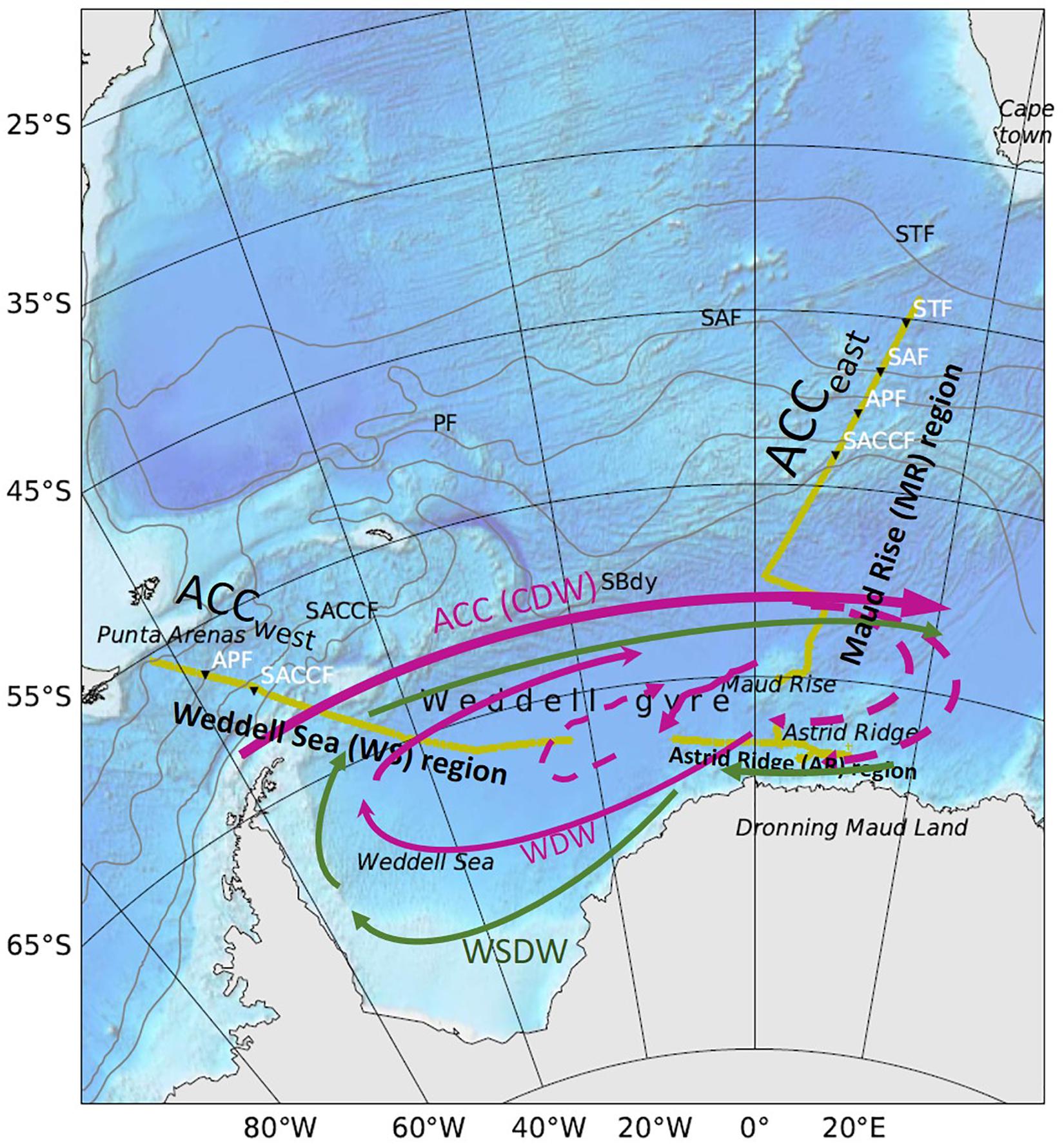
Figure 1. Study transect (yellow) with topography and trajectories of warm deep water (WDW, cyan), and Weddell Sea deep water (WSDW, green) modified after Hellmer et al. (2016). Gray lines: subtropical front (STF), subantarctic front (SAF), polar front (PF), South Antarctic circumpolar front (SACCF), and southern boundary (SBdy) are frontal positions as defined by Orsi et al. (1995). Solid black triangles are fronts identified along the study transect from the hydrographic data for this study.

This sea ice dynamic area is characterized by an abundant and persistent sea-ice cover that has extreme seasonal variability. The maximum extent of sea-ice cover occurs in September and by the following April, it would have shrunk to the third of the maximum extent (e.g., Vernet et al., 2019). Sea ice drift in dense pack ice and with icebergs are transported northward by the gyre. These melt in warmer waters and return freshwaters to the central gyre carrying micronutrients especially iron and stimulate primary productivity (Atkinson et al., 2001). The wind-driven, hydrodynamic circulation of the Weddell gyre connects the promontories (Astrid Ridge and Maud Rise) with the Weddell Sea on the west (Figure 1). The Weddell gyre makes the region the Weddell Sea deep water (WSDW) formation zone, as well as a region of upwelling (as a result of the interaction of the rise with the Weddell gyre) of warm deep water (WDW) also known as CDW (Hoppema et al., 1995; Fahrbach, 2006; Figure 1). The upwelling occurs particularly during austral autumn and winter periods (Gordon and Huber, 1990) through Ekman pumping. The biological productivity also can occur during sea ice cover due to the lowering of the sea ice concentration by upwelling of the WDW resulting in an ice-free ‘hole’ at the Maud Rise (Weddell polynyas) and near the Antarctic continent (coastal polynyas; Arrigo et al., 2008; Bakker et al., 2008; Cape et al., 2014; Vernet et al., 2019), which allows light to reach the surface ocean and stimulate primary productivity (Arrigo and Van Dijken, 2003). The upwelling of WDW tends to cause supersaturation of CO₂ in the surface, offset by biological drawdown decreases the surface ocean inorganic carbon levels (Fransson et al., 2004; Brown et al., 2015). The interplay between upwelling and biological production sets the source or sink characteristics in this region. Large seasonal changes in the surface CO₂ concentrations are observed due to the intense photosynthesis in summer and upwelling of deep waters during winter (Takahashi et al., 2014). Relative to other regions of the Southern Ocean, there are fewer sea surface CO₂ observations in the eastern and southern boundaries of the Weddell gyre. This is because of their remoteness and extreme conditions, especially during autumn/winter (e.g., Takahashi et al., 2009; Vernet et al., 2019). Figure 2 presents the sea surface fCO₂ observations available in SOCAT v-2020 (Bakker et al., 2016, 2020) from 1999 to 2019 showing the data available in the eastern and southern boundaries of the Weddell gyre are mostly just for one to 2 years. Enhanced observations of the nuanced interplay between physical and biological processes, at varying spatial and temporal scales in this data-sparse region of the Southern Ocean are required. Estimating the CO₂ fluxes will also require a thorough understanding of the processes controlling spatial and temporal variations.

FIGURE 2

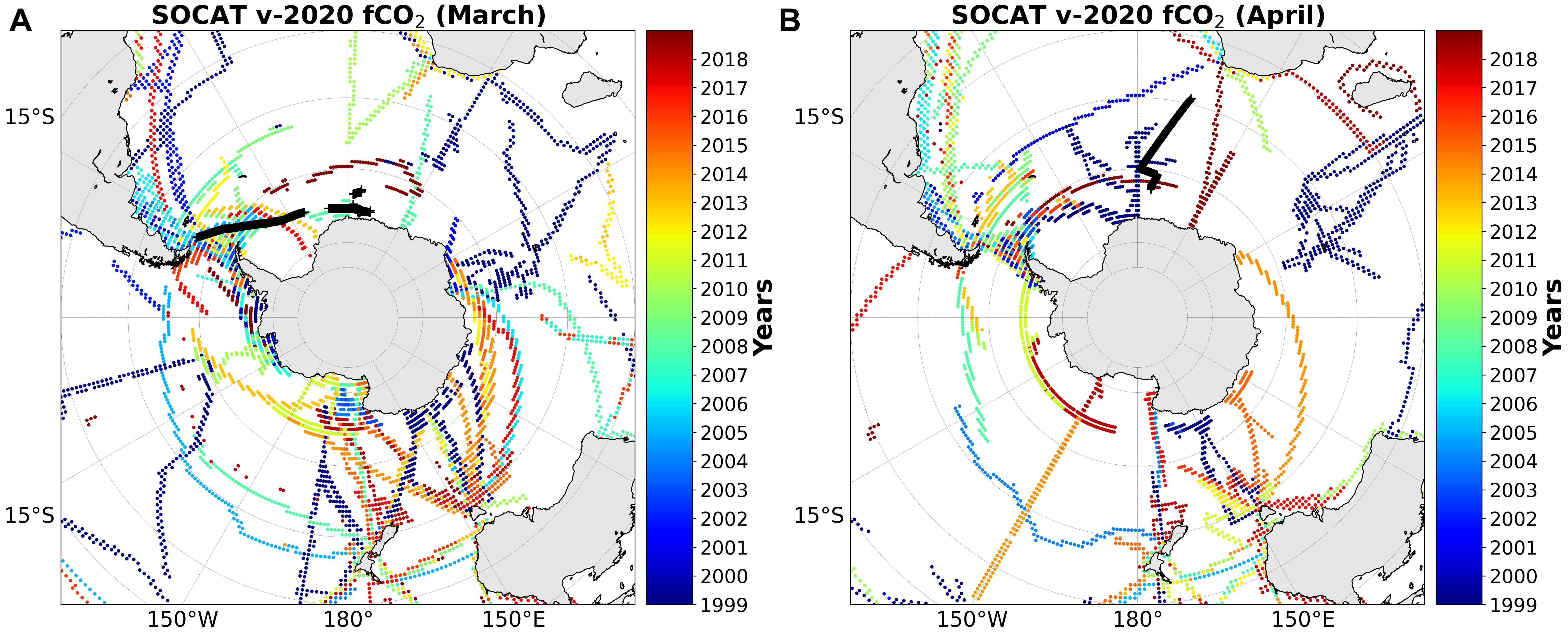
Figure 2. Map of available fCO₂ observations during autumn (March/April) in SOCAT v-2020 (Bakker et al., 2016, 2020) for the Southern Ocean from 1999 through 2019. Few years of observation are available in the Weddell gyre region the focus for this study (study transect; black color) relative to other regions in the Southern Ocean. (A) Years with available fCO₂ observations for March. (B) Years with available fCO₂ observations for April.

This study presents a unique dataset of surface water fCO₂, dissolved oxygen (DO), chlorophyll a, sea surface salinity, and temperature, and estimates on the air-sea CO₂ exchange characteristics in a large part of the Southern Ocean during austral autumn (February to April). The overarching aim of this study was to investigate the surface ocean property–property relationship to explain the physical and biological drivers controlling CO₂ fluxes in an area and season where few observations exist (see Figure 2).

Materials and Methods

Data and Calculations

The South Atlantic Southern Ocean was sampled between the 28th of February and the 10th of April 2019 onboard the Norwegian RV Kronprins Haakon. The study transect spanned from Punta Arenas (Chile) across ACC through the Weddell gyre to offshore of the Dronning Maud Land and Kong Håkon VII Hav at the Antarctic Coast. From there, heading northward along the 6°E meridian in the ACC toward Cape Town, South Africa (Figure 1; yellow transect) forms the eastern part of the transect. Underway continuous measurements were made for sea-surface and atmospheric CO₂ molar fractions (xCO₂) and ancillary parameters [sea-surface temperature (SST), sea-surface salinity (SSS), chlorophyll a fluorescence (chl^fluo) and DO]. Discrete seawater samples from Niskin bottles on a CTD rosette and from the ships’ water intake were also collected to supplement the dataset.

The dataset was divided into three sub-regions, categorized as the Weddell Sea (WS) region, Astrid Ridge (AR) region, and the Maud Rise (MR) region (Table 1 and Figure 1). This delineation was corresponded to the split along the transect (Figure 1) to ease the data analysis. The WS region span across part of the Weddell Sea in its southern extent and the ACC north of 60°S (ACCwest) in its northern extent (Figure 1). The AR region consists of the coastal waters near the Antarctic coast (66°S–68°S). Finally, the MR region spans the Weddell gyre in its southern extent to the north of 55°S in the ACC (ACCeast; Figure 1). The 60°S and 55°S are the northern boundary of the Weddell Gyre in the west and east, respectively (Deacon, 1979).

TABLE 1

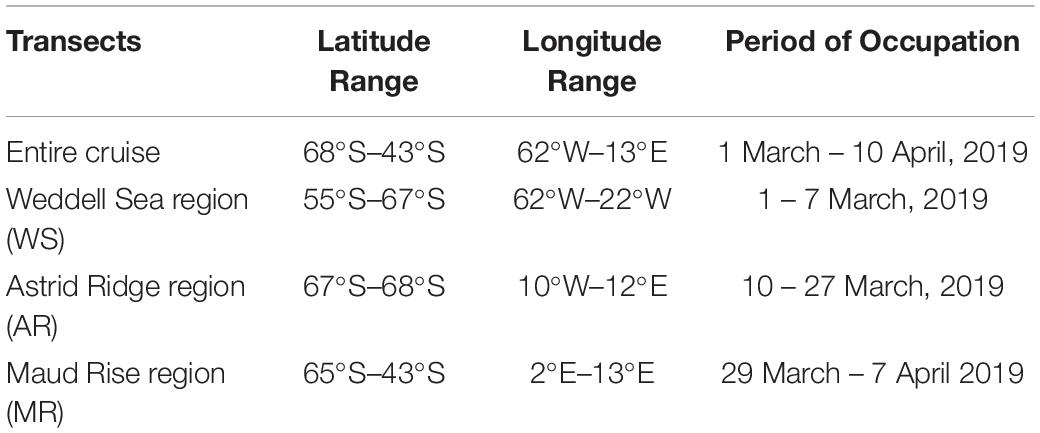
Table 1. Cruise transect and the three sub-regions defined with their coordinates.

Using hydrographic data from this study; oceanic fronts in the ACC were identified by characteristic property indicators based on criteria adopted from earlier works (Deacon, 1982; Orsi et al., 1995; Pollard et al., 2002; Chierici et al., 2004; Mattsdotter-Björk et al., 2014; Freeman, 2017; Strass et al., 2017). Four major fronts were indicated along the study transect (Figure 1, black solid triangles). The ACC fronts as defined by Orsi et al. (1995) are overlaid on the map (Figure 1, gray lines) with the study transect.

Fugacity of Carbon Dioxide

Sea surface and atmospheric CO₂ molar fractions (xCO₂) were measured onboard by an autonomous underway partial pressure of CO₂ (pCO₂) observation system (General Oceanics^®, Inc., model 8050) which consists of a gas-water equilibrating chamber and an infrared analyzer (LICOR^®, Model, 7000). The seawater was pumped from a side intake at 4 m below the sea surface, sprayed through the equilibration chamber; to equilibrate the CO₂ in the seawater with the air in the headspace of the chamber, and measured by the infrared analyzer, with an accuracy of ± 0.2 ppm. The analyzer was calibrated every 2.5 h using three standard gases in synthetic air with CO₂ molar fractions of 230, 400, and 550 ppm. The accuracy of the measurements by the General Oceanics system was estimated using secondary standards calibrated toward NOAA gases (traceable to WMO-x93 scale). Between calibrations, continuous measurements were made every third minute in a sequence of xCO₂ of standard gases, of air, and the seawater. The sea surface water and atmospheric fugacity of CO₂ (fCO₂ssw and fCO₂atm) were computed from the xCO₂ through pCO₂ corrected for non-ideal behavior using SST and SSS following the methods of Pierrot et al. (2009) for fCO₂ssw and with Lencina-Avila et al. (2016) for fCO₂atm. For an uncertainty in the measured standards of less than 1 ppm (reflecting the standard deviation of the difference between measured standards and certified values), with an accuracy in the equilibrator temperature of 0.01°C, (0.009°C at 0°C water temperature) and at the intake temperature of 0.001°C, the determined fCO₂ will be within 2 μatm as previously stated by Pierrot et al. (2009). This assumes that the pressure is determined within 0.2 hPa.

Sea-Air Carbon Dioxide Flux Calculations

Sea-air CO₂ flux (FCO₂) was calculated using equation (1):

$${\text{FCO}}_2=k\times s\times \mathrm{\Delta }{\text{fCO}}_2(1)$$

where

$$\mathrm{\Delta }{\text{fCO}}_2={\text{fCO}}_2\text{ssw}-{\text{fCO}}_2\text{atm}(2)$$

k is the CO₂ gas transfer velocity coefficient (cm hr^–1) estimated using the formulation of Wanninkhof (2014) with the coefficient factor of 0.251 and a quadratic wind speed. Co-location wind speed recorded at 36 m height from the ship’s scientific data and corrected to a 10 m standard height was utilized.

s is the CO₂ solubility coefficient (mol L^–1atm^–1) calculated following the equation and the coefficients for temperature and salinity dependence of the solubility of CO₂ in Weiss (1974). ΔfCO₂ equals the sea-air fCO₂ gradient in μatm. The recalculated fugacity of CO₂ from the continuous underway measured mole fractions for the atmospheric CO₂ (Supplementary Figures 1A,B), was used in equation (2) for fCO₂atm in the calculations for all the regions. The flux values are reported in mmol m^–2 d^–1 using a conversion factor of 0.24, taking into account the μatm, the conversion of cm h^–1 to m d^–1 and mol L^–1 atm to mol m^–3 atm.

Negative values of ΔfCO₂ represent the undersaturation of fCO₂ssw with respect to the atmospheric fCO₂ (fCO₂atm) and positive values represent supersaturation. The sea surface water is saturated with fCO₂ when ΔfCO₂ is 0. Similarly, negative values of FCO₂ quantify the flux of CO₂ into the ocean while positives values indicate the degassing of CO₂ to the atmosphere. At equilibrium, FCO₂ is 0.

The fugacity of CO₂ saturation (fCO₂sat) was calculated using the following equation:

$${\text{fCO}}_2\text{sat}=\frac{{\text{fCO}}_2\text{ssw}}{{\text{fCO}}_2\text{atm}}\times 100(3)$$

Sea Surface Temperature and Salinity

Continuous SST and SSS measurements were obtained by a thermosalinograph (SeaBird SBE21 TSG) and an additional temperature sensor (SBE38) at the seawater intake at the bottom of the ship, with an accuracy of ± 0.001°C. The accuracy of the salinity sensor of ± 0.02 psu was obtained by comparison with salinity measured using an Autosal^® on discrete water samples collected from the intake and the drift corrections obtained from calibrations of the sensor.

Dissolved Oxygen, Oxygen Saturation, and Apparent Oxygen Utilization

Dissolved oxygen concentration ([O₂], μmol kg^–1) was measured with the Aandera optode (model 4330, the accuracy of < ± 2%) sensor attached to the seawater intake, corrected for SSS. The optode DO values were evaluated by Winkler titration of water samples collected at 5–10 m depth from Niskin-CTD rosette and water intake, resulting in uncertainty of 2 ± 1%. Percentage oxygen saturation (O₂sat) and apparent oxygen utilization (AOU) were estimated using Eqs (4) and (5; Garcia et al., 2013), respectively.

$${\text{O}}_2\text{sat}=\frac{[{\text{O}}_2]}{[\mathrm{O}^{\prime }{}_2]}\times 100(4)$$

$$\text{AOU}=[\mathrm{O}^{\prime }{}_2]-[{\text{O}}_2](5)$$

[O’₂] is the O₂ solubility concentration (μmol kg^–1) calculated as a function of in situ temperature, salinity, and one atmosphere of the total pressure. The values of [O’₂] were calculated according to Garcia and Gordon (1992) based on the values of Benson and Krause (1984).

The AOU of a water sample is the difference between the concentration at oxygen saturation and the measured oxygen concentration in the water with the same physical and chemical properties. AOU is commonly used to investigate the sum of the biological activity that the sample has experienced since it was last in equilibrium with the atmosphere. At 100% O₂sat, AOU is 0. High oxygen utilization results in O₂sat < 100 and AOU > 0, while low oxygen utilization results in O₂sat > 100 and AOU < 0. Thus, positive AOU will depict the respiration/remineralization process and negative AOU will depict photosynthesis.

Chlorophyll a

Underway chlorophyll a fluorescence (chl^fluo) was measured with the Wetstar fluorometer every minute. The fluorometer was calibrated against a total of 109 chl-a measurements (chlextr) obtained from discrete samples, which were collected and analyzed after extraction using the acetone-spectrofluorometric method (Holm-Hansen and Riemann, 1978). Supplementary Figure 2A shows the diurnal (day and night) fluorescence derived chl-a which does not show a significant difference in the slope and intercept hence the combined data (Supplementary Figure 2B) was used for the calibration. Therefore, the linear correlation obtained between the combined diurnal WetStar sensor fluorescence and the extracted chl a, (r² = 0.85, N = 109) was used to convert the voltage signal (mV) to in situ chl-a:

$$\mathrm{chl}-\mathrm{a}=(0.09\times \text{fluorescence})+0.06(6)$$

Results

Physical Properties and Hydrography

Temperature ranges within the WS, AR, and MR regions were −0.9 to 6.19°C, −1.9–0.4°C, and −0.1–14.0°C, respectively (Table 2). SSS values were in the range of 33.26–34.46 psu, 33.45–34.25 psu, and 33.74–35.10 psu for the respective regions (Table 2). SST varied widely over the WS and MR regions with mean values and standard deviations of 1.1 (± 2.0)°C and 1.9 (± 3.1)°C, respectively, indicating the difference between warmer characteristics of ACC waters and the colder and more stratified water in the Weddell gyre. In the AR, temperature showed relatively small variability, the mean SST was -0.7 (± 0.7)°C (Table 2).

TABLE 2

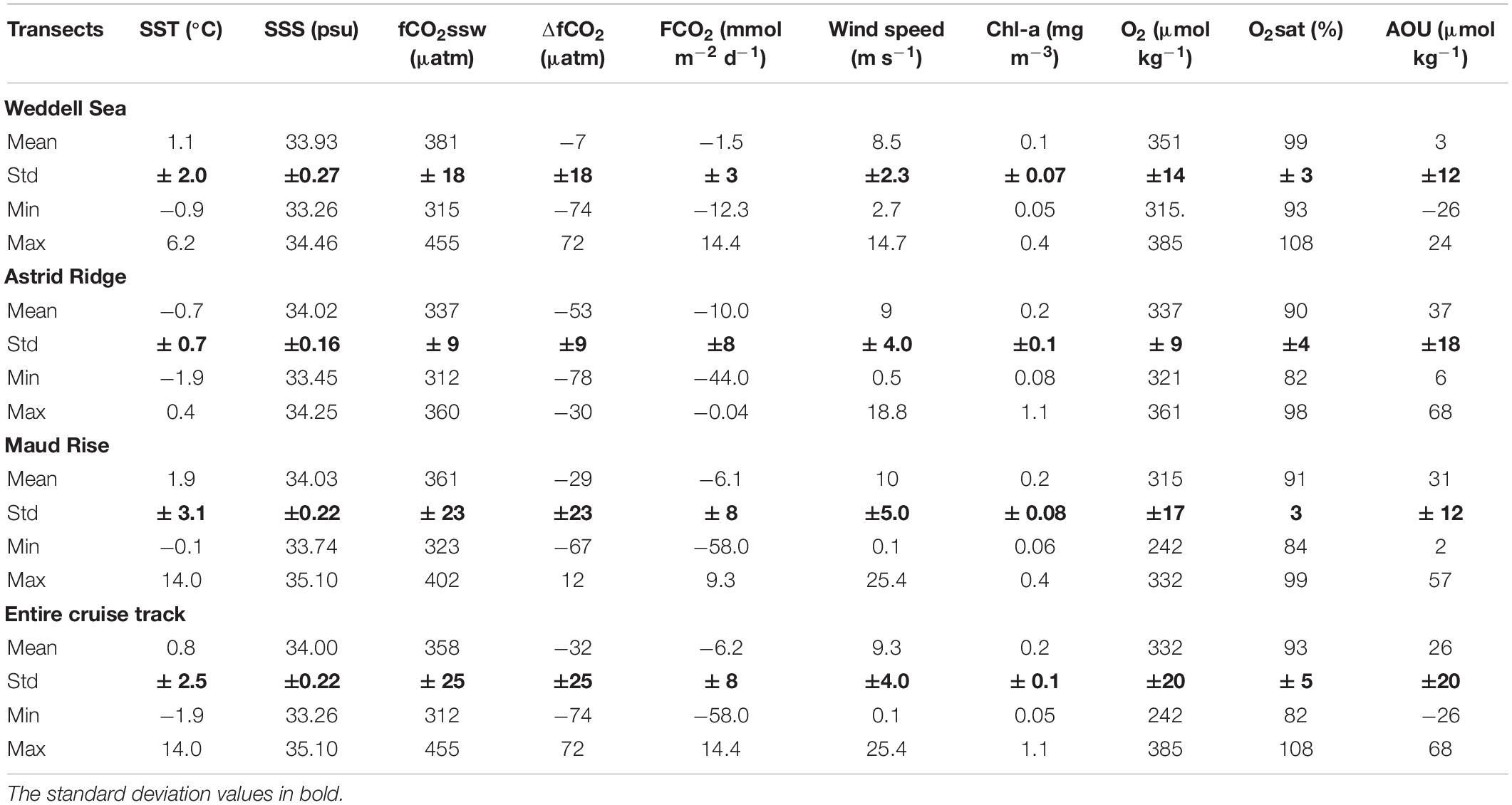
Table 2. Mean values, standard deviation (Std) (± 1σ), minimum (min), and maximum (max) values of the measured and calculated parameters in the defined regions in the study area.

The frontal systems described for the studied region are identifiable from the sharp gradient created by the most rapid changes in SST and SSS. For instance, while going southwards across ACCwest in the WS region, at 57.5°S, the SST and SSS rapidly decreased from 6 to 3°C and from 34.1 to 33.75 psu, respectively (Figure 3A), indicating the location of the Antarctic Polar Front (APF) on the western flank of the cruise track. A decrease in SST to about 1°C with an increase in SSS from 33.8 psu to 34.0 psu at around 59°S appears to be an expression of Southern ACC Front (Figure 3A, SACCF). Moving northward from AR on the eastern flank of the transect, SACCF was also identified at 53.25°S by the SST increase from below 1 to about 4°C with the corresponding decrease in the SSS from 34.0 psu to 33.8 psu (Figure 3C, SACCF) in the MR region. A weak northward increase of SST from below 4°C to about 5°C between 51 and 50°S shows an expression of APF (Figure 3C) and a northward increase of SST from 5 to 8°C with an increase in SSS from 33.70 to 33.80 psu indicating the Sub-Antarctic Front at 48.2°S (Figure 3C, SAF). The large sharp increase of SST and SSS from 8.5 to 14°C and from 33.9 to 35.10 psu, respectively, with warmer (greater than 11.5°C) and saltier (greater than 34.9 psu) waters on the northern side indicated the Subtropical Front at 45.28°S (Figure 3C, STF). STF was further south than the other fronts indicated for this study compared with the Orsi et al. (1995) frontal positions along the transect.

FIGURE 3

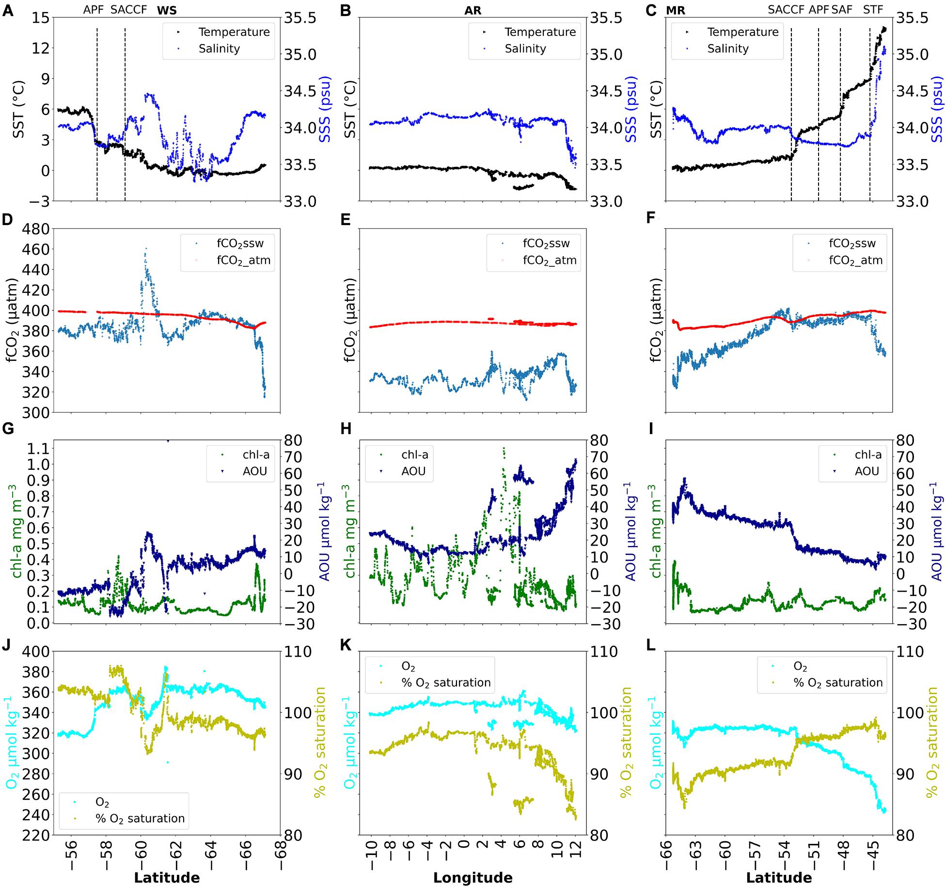
Figure 3. Spatial distributions of sea surface fugacity of CO₂ with physical and biological parameters. Column 1: (A,D,G,J) WS region, Column 2: (B,E,H,K) AR region, and Column 3: (C,F,I,L) MR region. The red color represents the distributions of the atmospheric fugacity of CO₂ in each of the defined regions.

Spatial Distribution of fCO₂ssw, With the Physical and Biological Parameters

WS Region

The fCO₂ssw distributions in the WS region ranged from 315 to 455 μatm (Table 2). The WS region showed the largest spatial variability of fCO₂ssw relative to other regions (Figure 3D) and included, the highest fCO₂ssw of 455 μatm recorded on the cruise in the WS region south of the SAACF, between 60 and 62°S, accompanied by a large increase in SSS, a small decrease in the SST and a small increase in chl-a (Figures 3A,D,G). Increasing fCO₂ssw toward saturation relative to the mean fCO₂atm also corresponded with increasing SSS in the SACCF (Figures 3A,D). The highest chl-a concentration (0.4 mg m^–3) in this region was found between 58 and 59°S (Antarctic zone; Figure 3G). South of 66°S the fCO₂ssw drastically decreased to the minimum value of 315 μatm, which coincided with a peak in chl-a of about 0.35 mg m^–3 (Figures 3D,G) and low temperatures. However, DO concentration variation only corresponded partly to the variability in the chl-a concentration. This was particularly clear in the APF and south of 66°S where no correlation between chl-a and DO was observed (Figures 3G,J). Opposite variation of AOU with DO saturation was observed as expected (Figures 3G,J), whereas there are deviations in the co-variation between the DO and oxygen saturation in the APF and SACCF region (Figure 3J).

AR Region

Along coastal longitudes of the AR region (Figure 1, Astrid Ridge region), all parameters showed less variability, except for chl-a which showed several peaks (Figure 3H) with an uneven fCO₂/chl-a relationship for photosynthesis (Figures 3E,H). For example, a chl-a concentration of 1.1 mg m^–3 coincided with a fCO₂ssw value of about 320 μatm as well as chl-a concentrations between 0.2 and 0.6 mg m^–3 as observed at 5°W and 2°W. Moreover, some values of fCO₂ssw were lower than 320 μatm and coinciding with chl-a concentrations of about 0.2–0.4 mg m^–3 at 7°E (Figures 3E,H). Low values of fCO₂ssw, SST, and SSS with high values of chl-a were recorded in this region (Figures 3B,E,H). AOU also showed the opposite variation to DO saturation (Figures 3H,K) and DO and oxygen saturation generally co-varied in this region (Figure 3K).

MR Region

In the MR region, fCO₂ssw showed large variability as indicated by the standard deviation of ± 23 μatm (Table 2). The lowest fCO₂ssw values in the south coincided with high chl-a and the lowest SST (Figures 3C,I). The fCO₂ssw increased northward and reached oversaturation at about 55°S, coinciding with increased SST and fCO₂ssw variability that coincided partly with the fronts (Figures 3C,F,I). The northward warming at the fronts corresponded to increasing fCO₂ssw, leading to fCO₂ oversaturation with an exception at the STF where warming corresponded to a decrease in fCO₂ssw and increased chl-a. AOU showed opposite variation to DO saturation (Figures 3I,L) and DO and oxygen saturation co-varied except for north of 54°S in the frontal waters (Figure 3I).

Spatial Distribution of FCO₂, ΔfCO₂, and Wind Speed

The spatial distribution of the sea-air CO₂ flux (FCO₂, mmol m^–2d^–1), ΔfCO₂ (μatm), and the co-location wind speed (m s^–1) from the ship data corrected to 10 m standard height, for the three defined regions are presented in Figure 4. Negative FCO₂ denotes a CO₂ flux into the ocean (CO₂ influx; sink) and positive values denote CO₂ flux out of the ocean to the atmosphere (CO₂ outgassing; source). The FCO₂ spatial distribution along the entire cruise varied from the largest CO₂ outgassing (source) of 14.4 mmol m^–2d^–1 between 60 and 62°S in the WS region to a large CO₂ sink of −58.0 mmol m^–2d^–1 at the Maud Rise in the MR region (Table 2 and Figures 4A,C). The colocation wind speed along the entire cruise varied from near zero wind speed of 0.1 m s^–1 to a maximum wind speed of 25.4 m s^–1 (Table 2) with mean values for each region being 8.5 (± 2.3) m s^–1, 9 (± 4) m s^–1 and 10 (± 5) m s^–1 (Table 2) for WS, AR, and MR, respectively. Despite occasions of CO₂ outgassing along the transect in the WS and MR region (Figures 4A,C), both regions showed an average ocean CO₂ uptake of −1.5 mmol m^–2 d^–1 and −6.1 mmol m^–2 d^–1 (Table 2) respectively and as well as the AR region where CO₂ influx was observed throughout the region (Figure 4B). The AR region showed the largest average sink for atmospheric CO₂ with an average flux estimate of −10.0 mmol m^–2 d^–1 (Table 2).

FIGURE 4

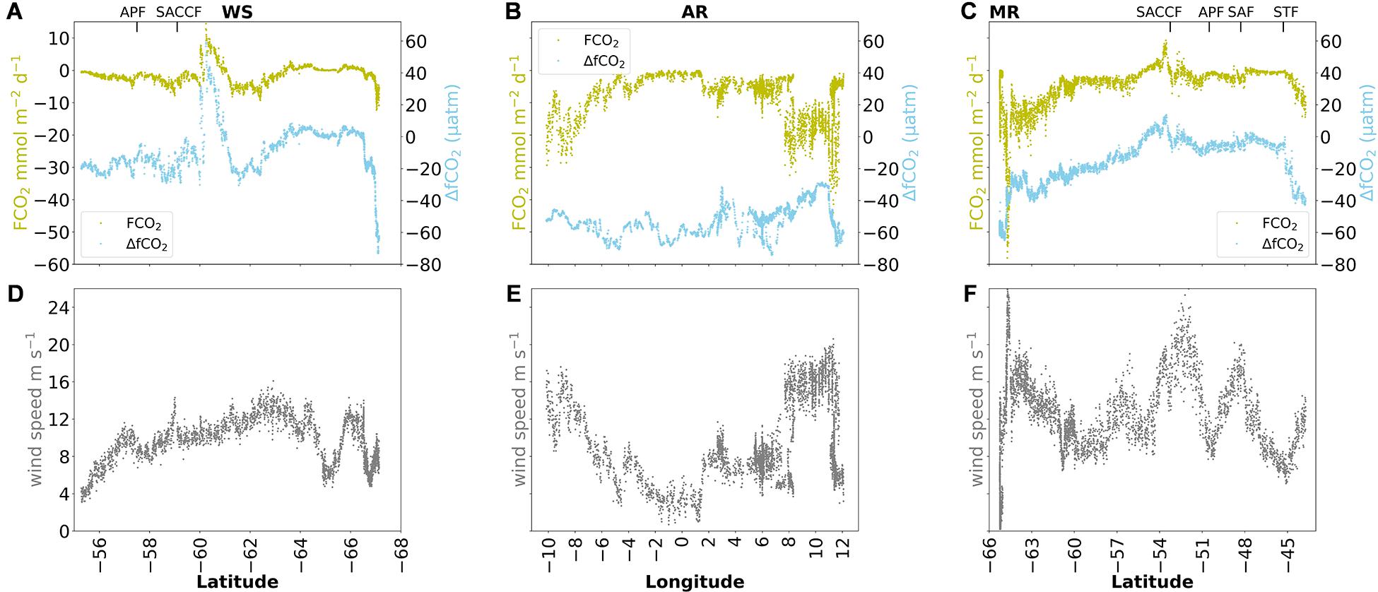
Figure 4. Spatial distributions of CO₂ flux (FCO₂, mmol m^–2 d^–1) with the sea-air gradient of fCO₂ (ΔfCO₂, μatm) and wind speed (m s^–1). Column 1: (A,D) WS region, Column 2: (B,E) AR region, and Column 3: (C,F) MR region.

In the WS region, FCO₂ showed a similar spatial variation pattern with ΔfCO₂ (Figure 4A). The large CO₂ outgassing in the WS coincided with the highest positive ΔfCO₂, with little change in the wind speed (Figures 4A,D). However, the largest undersaturation (largest negative ΔfCO₂) in the southernmost part at 67°S did not result in the expected higher CO₂ influx, a consequence of the relatively low wind speed (Figure 4D).

The AR region showed uptake of CO₂, which generally increased with increasing wind speed (Figures 4B,E). Also, here between 3°W and 1°E, the CO₂ influx did not correspond with the large undersaturation of fCO₂ssw (large negative ΔfCO₂, Figure 4B) where the CO₂ influx was nearly zero regardless of the large undersaturation of fCO₂ssw of about −60 μatm (Figure 4B). This also corresponded to the relatively low wind speed values recorded along this longitude (Figure 4E).

Moving northward in the MR region to 60°S, increasing wind speed as well as the magnitude of undersaturation of fCO₂ssw (large negative ΔfCO₂) resulted in larger CO₂ flux. However, between 60 and 57°S, the FCO₂ showed little change although both ΔfCO₂ and wind speed increased (Figures 4C,F). North of 57°S, FCO₂ showed a similar spatial variation pattern with ΔfCO₂ and higher wind speeds seemed to favor CO₂ outgassing between 52 and 48°S (Figures 4C,F). The highest wind speed of 25.4 m s^–1 recorded on the cruise was found along the latitudes of 52°S and around 65°S (Figure 4F). An increasing CO₂ influx with larger negative gradients of ΔfCO₂ and increasing wind speed was observed north of STF in the subtropical waters (Figures 4C,F).

Discussion

This study presents a recent sea-air CO₂ flux estimate from direct CO₂ observations in the Atlantic sector of the Southern Ocean and within the Weddell gyre region. From the observations performed in autumn, the whole region along the study transect acted as an average ocean CO₂ sink for atmospheric CO₂ with an average FCO₂ of −6.2 (± 8) mmol m^–2 d^–1 (Table 2). The Weddell gyre region showed a strong uptake of atmospheric CO₂ at the Maud Rise feature and near the Antarctic coast at the Astrid Ridge region and strong outgassing around 60°S. Integrating the CO₂ uptake for the Weddell gyre region, a flux value of −6.9 (± 8) mmol m^–2 d^–1 was obtained. Due to low CO₂ data coverage in this region during autumn (see Figure 2), few sea-air CO₂ flux estimates from direct sea-surface observations for the Weddell gyre region are available with which to compare the values estimated in this study. Hoppema et al. (2000) calculated a mean flux of −2.5 mmol m^–2 d^–1 for the autumn period March/May 1996 for the Weddell gyre region integrated over different subregions (in the western Weddell gyre, along the prime meridian, and the eastern Weddell gyre). The flux of −6.9 mmol m^–2 d^–1 obtained for this study indicates higher uptake of CO₂ in the region than previously estimated. Correspondingly, climatological monthly sea-air fluxes at a 4°lat × 5°long box resolution for the reference year 2000 (Takahashi et al., 2009) integrated over the Weddell gyre for the same months (March and April) as this study, yielded a flux of −1.8 mmol m^–2 d^–1. However, the paucity of spatial and temporal CO₂ observations for this region during autumn and for which space-time interpolation of available observations was used for the climatological flux estimate does not allow for a plausible comparison with the estimated value in this study. Nevertheless, sea-air fCO₂ disequilibrium (ΔfCO₂) in the study region estimated from sea−surface fCO₂ measurements from 2009 to 2018 in the SOCAT v-2020 database (Bakker et al., 2016, 2020), compared to the ΔfCO₂ calculated from this study during the same period (March and April) also show higher uptake of CO₂ in the overall, during this study than in the previous years (2009–2018; Supplementary Figure 3). Also, the mean values of fCO₂ssw estimated from available fCO₂ observations in the SOCAT v-2020 during the same period for this study, ranging from 2–8 years shows a higher fCO₂ssw in the surface ocean for this study for most of the region where observations are available for comparison (Supplementary Figures 4A,B). The anomaly plot (fCO₂ssw from this study minus mean fCO₂ssw from the SOCAT v-2020; Supplementary Figure 4C) show a higher fCO₂ssw for this study with the difference ranging from ca 20 to 120 μatm in the Weddell Sea and a lower fCO₂ssw of ca 20 μatm in the AR region which perhaps is due to the higher chl-a concentrations observed in this study (see Figure 3H). This shows the higher CO₂ uptake by surface oceans during this study relative to the SOCAT climatology-based estimates.

Regional Drivers of FCO₂

Carbon dioxide flux (FCO₂) in the surface ocean is primarily driven by ΔfCO₂ and wind speed. The ΔfCO₂ is affected by changes in temperature (SST), salinity (SSS), processes in the surface ocean that consume CO₂ (photosynthesis), or produces CO₂ (respiration), or upwelling of CO₂-rich waters at fronts and promontories that increases surface ocean fCO₂ in the Southern Ocean. Moreover, sea-ice formation and melting and processes within sea ice also affect the CO₂ flux by the changes in fCO₂ssw (e.g., Fransson et al., 2011).

The net uptake flux [−6.2 (± 8) mmol m^–2 d^–1] for this study was predominantly influenced by primary production leading to a large undersaturation of fCO₂ssw relative to the atmosphere in the AR and the MR region. A combination of greater stratification due to sea ice melt, increased light in summer with possible ice melt iron fertilization enhances biological CO₂ drawdown (Atkinson et al., 2001; Chen et al., 2011) in the study region. The biological CO₂ drawdown continues into autumn with ongoing primary production at the late stage (Brown et al., 2015). This could explain the high chl-a concentrations within the AR and MR regions for this study (Section “Spatial Distribution of fCO2ssw, With the Physical and Biological Parameters”). Also, the autumn bloom was observed in the upper water column west of the Astrid Ridge during the cruise for this study (Kauko et al., in review).

The WS region acted both as a weak sink and a weak source with an average FCO₂ of −1.5 (± 3) mmol m^–2 d^–1. The large variability was associated with the large fCO₂ssw supersaturation, fCO₂ outgassing between 60 and 62°S, and the low CO₂ influx found in the SACCF (Figure 4A). This may result from the upwelling in the region indicated by an increase in the SSS (Figure 3A). Upwelled deep waters are older and relatively rich in CO₂ from the remineralization of organic carbon in the deep (Gordon and Huber, 1990; Hoppema et al., 2000; Fransson et al., 2004). Once at the surface, they begin to equilibrate with the atmosphere driving CO₂ outgassing (Metzl et al., 2006; Gruber et al., 2009). Interestingly, the high fCO₂ssw is also seen at the same latitude north of the Peninsula in the SOCAT v-2020 for the number of available fCO₂ observations (Supplementary Figures 4A,B). This is likely a permanent local event as the area is known for intense upward mixing of cold deep waters (Heywood et al., 2002, 2004) which may be linked with the bathymetry interaction with the high rising South Scotia Ridge in the Scotia Sea in this region. The large CO₂ influx observed south of 67°S (Figure 4A) can be attributed to upwelling-induced primary production. This is because the large undersaturation of fCO₂ssw relative to the atmospheric CO₂ in Figure 3D corresponded to an increase in SST and high SSS (upwelling) (Figure 3A), and increased chl-a (primary production; Figure 3G). The course of the WDW from the western part of the Weddell gyre (Figure 1), supports the upwelling of WDW (increase in SST and high SSS) in the region.

The largest average regional CO₂ sink of −10.0 mmol m^–2 d^–1 (Table 2) was estimated for the AR region in the far south along the Antarctic coast. The sink was associated with the high chl-a concentrations recorded in this region (Figure 3H) which likely caused the undersaturation of fCO₂ssw (Figure 4B; ΔfCO₂). Therefore, the high ocean uptake of CO₂ could be attributed to primary production in combination with the effect of wind speed; since CO₂ influx also increased once the wind speed increases such as at 10°E (Figures 4B,E).

Maud Rise region was a stronger average CO₂ sink than the WS region and has an average FCO₂ of −6.1 (± 8) mmol m^–2 d^–1 (Table 2). The MR region spans from the Weddell gyre at the Maud Rise to the ACC and subtropical waters north of the STF (Figure 1). The net sink in this region was greatly influenced by the large CO₂ uptake at the Maud Rise and in the subtropical waters (Figure 4C). The Maud Rise has been identified by many other authors as an area of high primary productivity which results in a large biological CO₂ drawdown. Formation and upwelling of WDW (Gordon and Huber, 1990; Hoppema et al., 1999), interacting with the Maud Rise brings nutrients and CO₂ to the surface and drives productivity (Holm-Hansen et al., 2005). Indeed, the observed increase in SSS and SST (upwelling of WDW) at the Maud Rise latitude (65°S; Figure 3C) and the corresponding increase in the chl-a concentration (Figure 3I) supports the observed net CO₂ sink. The CO₂ outgassing in the ACC component of the MR region is associated with high wind speeds at the fronts and enhanced deep upwelling, driven by the strong westerly winds (e.g., Fransson et al., 2004; Brown et al., 2015). At the most northern extent of the MR region (north of the STF; Figure 3, column 3), the low values of DO, chl-a, and fCO₂ssw are characteristics of oligotrophic subtropical waters. Enhanced transport of dissolved organic carbon from the surface to the deep ocean has previously been observed in the oligotrophic subtropical oceans (Roshan and DeVries, 2017). This could potentially translate to the fCO₂ssw observed in the region (Figure 3F) and which results in the large undersaturation of fCO₂ssw (ΔfCO₂) and subsequent high FCO₂ (Figure 4C). Hoppema et al. (2000) also recorded undersaturated surface water for CO₂ and observed that the surface water in the region tends to flow northwards to participate in the formation of Antarctic Intermediate Water (AAIW) and so constitute a conduit for CO₂ uptake from the atmosphere. Other sea-surface fCO₂ observations in this region during April/May of the same year (2019) as this study also show low fCO₂ for the same region near the STF and similar fCO₂ distributions overall for the region of study (Supplementary Figure 5). This corroborates the autumn distribution of sea surface fCO₂ in the region for 2019 as presented in this study.

Regional Drivers of fCO₂ssw Using a Correlation Model

Dissolved O₂ can help to constrain understanding of the drivers of surface ocean carbon dynamics. To explain the nuanced interplay of the various drivers influencing the fCO₂ssw variability, a correlation model between the saturation of fCO₂ (fCO₂sat) and O₂ saturation (O₂sat) relative to the atmosphere as utilized by Carrillo et al. (2004) was explored (Figure 5). In the model, the calculated fCO₂sat and O₂sat (see Sections Sea-Air Carbon Dioxide Flux Calculations and Dissolved Oxygen, Oxygen Saturation, and Apparent Oxygen Utilization) were correlated and used as an index to derive the controlling or dominant chemical, physical and biological processes influencing fCO₂ssw variability.

FIGURE 5

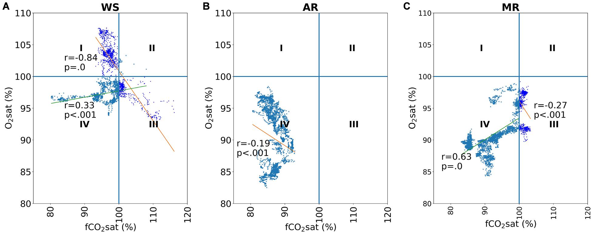
Figure 5. Percentage O₂ saturation (O₂sat) versus percentage fCO₂ (fCO₂sat) for the three regions. (A) WS region, (B) AR region, and (C) MR region. Vertical and horizontal sky-blue lines represent 100% saturation levels fCO₂ssw and O₂, respectively. Intersection points of the two lines denote the origin and 100% air-saturation of fCO₂ and O₂. I, II, III, IV represent the four quadrants. Distribution of observations driven dominantly by photosynthesis (in I) and respiration/remineralization and/or upwelling (in III) are represented by deep blue colors while those driven dominantly by warming/cooling effect (in II and IV) are represented by sky blue color.

The correlative exercise segregated the fCO₂ and O₂ data into four quadrants (Carrillo et al., 2004; Moreau et al., 2013) depicting four case waters (Figure 5). The distribution of observations in each quadrant helps infer the dominating processes controlling fCO₂ssw distribution in surface waters. Quadrant I depicted surface waters of simultaneous fCO₂ undersaturation (below 100% saturation level) and O₂ supersaturation (above 100% saturation level), implying photosynthesis dominantly driving the spatial distribution of fCO₂ssw. In Quadrant II, supersaturation of both O₂ and fCO₂ suggests warming of the surface waters as the dominant process increasing the saturation of both fCO₂ and O₂. Quadrant III depicted surface waters experiencing simultaneous fCO₂ supersaturation and O₂ undersaturation and implies dominant respiration/remineralization or upwelling of respired subsurface waters. Lastly, quadrant IV depicted surface waters of simultaneous fCO₂ and O₂ undersaturation which implies the cooling effect of temperature dominantly driving both fCO₂ and O₂ saturation in the surface water lower with respect to gas exchange. Consequently, if biological processes (primary production and respiration/remineralization) and upwelling are the dominant drivers controlling fCO₂ssw and O₂ saturation, a negative correlation will be expected with the O₂sat and fCO₂sat values distributed linearly through quadrant I and III in Figure 5. Also, if temperature-driven processes (warming and cooling) are the dominant control factor for fCO₂ssw and O₂ saturation, a positive correlation between O₂sat and fCO₂sat with the values distributed linearly through quadrant II and IV will be expected in Figure 5. The process vectors (correlation lines) in Figure 5 show deviations in correlative relationships, potentially indicating a more complex interplay between the processes driving the observed distribution of fCO₂sat and O₂sat. This is illustrated in Sections “Surface Water Property–Property Relationship With fCO₂sat/O₂sat Correlations for Case Waters QI and QIII” and “Surface Water Property–Property Relationship With fCO₂sat/O₂sat Correlations for Case Waters QII and QIV” as the spatial distributions of the fCO₂sat/O₂sat for the quadrants are described relative to the surface water properties of controlling variables (chl-a, AOU, SST). For example, increasing chl-a, a proxy for primary production, results in the consumption of CO₂ with the release of oxygen in the surface waters (Sigman and Hain, 2012) affecting their respective saturation levels. Negative values of AOU indicating low oxygen utilization corresponds to the photosynthetic process, while positive values of AOU indicate respiration/remineralization and upwelling. Likewise, an increase in temperature produces an increase in both the O₂ and fCO₂ saturation state. SSS is used as an index for upwelling since upwelled waters are more saline. Deviations in the correlative relationships could also be due to the difference in sea-air gas exchange rates for O₂ and fCO₂ (Broecker and Peng, 1983) or due to the formation and dissolution of calcium carbonate (Dieckmann et al., 2008). Since fCO₂ssw is a component of the ocean’s buffer system, the sea-air CO₂ exchange has a slower response than the case for oxygen with timescales ranging from days to weeks for O₂ and months for fCO₂ [details of the sea-air exchange model for O₂sat and fCO₂sat in Carrillo et al. (2004)]. Thus, the processes of differential sea-air gas exchange will affect the O₂sat/fCO₂sat ratio. The case waters depicted by the quadrants are hereafter referred to as QI, QII, QIII, and QIV.

Surface Water Property–Property Relationship With fCO₂sat/O₂sat Correlations for Case Waters QI and QIII

The case waters QI representing photosynthesis were found only in parts of the WS region; in the ACCwest on its northern extent and a small section on the southern extent in the Weddell gyre (Figure 6, yellow). The effect of photosynthesis on the fCO₂ssw distribution in this region confirms previous studies within the same region especially in the east of Drake Passage (Munro et al., 2015). QIII case waters representing respiration/remineralization and upwelling were found predominantly in the MR region (in the ACCeast) and some part of the WS region (in the Wedell gyre; Figure 6, deep blue). The fCO₂sat/O₂sat correlation for the QI and QIII in the WS region showed a significant negative correlation of −0.84, p < 0.001 with a slope of −0.78 (Figures 5A,I,III). This strong association between fCO₂sat and O₂sat indicated the combined influence of the biological and upwelling processes driving the observed fCO₂sat/O₂sat variability. Figure 7A presents the fCO₂sat/O₂sat variability for the case waters in QI and QIII. North of 60°S in the ACC and between 61 and 62°S in the Weddell gyre (Figure 3G), the variability in the chl-a concentrations, and the AOU (negative AOU) highlighted the photosynthetic relationship of fCO₂sat/O₂sat in the same region (Figure 7A). Between 60 and 61°S and South of 63°S along the same transect, upwelling of high saline (Figure 3A) and CO₂-rich waters (Figure 3D) with respiration/remineralization (positive AOU, Figure 3G) were evident from the corresponding supersaturation of fCO₂sat and the undersaturation of O₂sat (Figure 7A). The positive values of AOU and increase in SSS in this region, support the respiration/remineralization and upwelling processes driving the observed fCO₂sat/O₂sat here. The transition to supersaturation and a local maximum of fCO₂ssw between 60 and 61°S along the WS transect also previously observed near the same region (Stoll et al., 1999; Hoppema, 2004) was attributed to possible in situ remineralizations of organic matter. Besides, the area is known for intense upward mixing of cold deep waters (Heywood et al., 2002, 2004). Southward of 63°S, the observed values of chl-a concentration (Figure 3G) suggest an interplay of photosynthesis with the upwelling process shown for the region by the fCO₂sat/O₂sat distributions (Figure 7A). It is thought that photosynthesis offsets the fCO₂sat while enhancing the O₂sat and was evident in the slight supersaturation of fCO₂sat and the near-saturation level (close to 100% saturation) of O₂sat (Figure 7A) in the region. In the ACC, north of the APF the SST and SSS show a similar variation pattern (Figure 3A) to the fCO₂sat (Figure 7A) while at the APF both fCO₂sat and O₂sat decreases with decrease in SST and SSS (Figures 3A,7A). This also shows the interplay of temperature with photosynthesis in QI case waters.

FIGURE 6

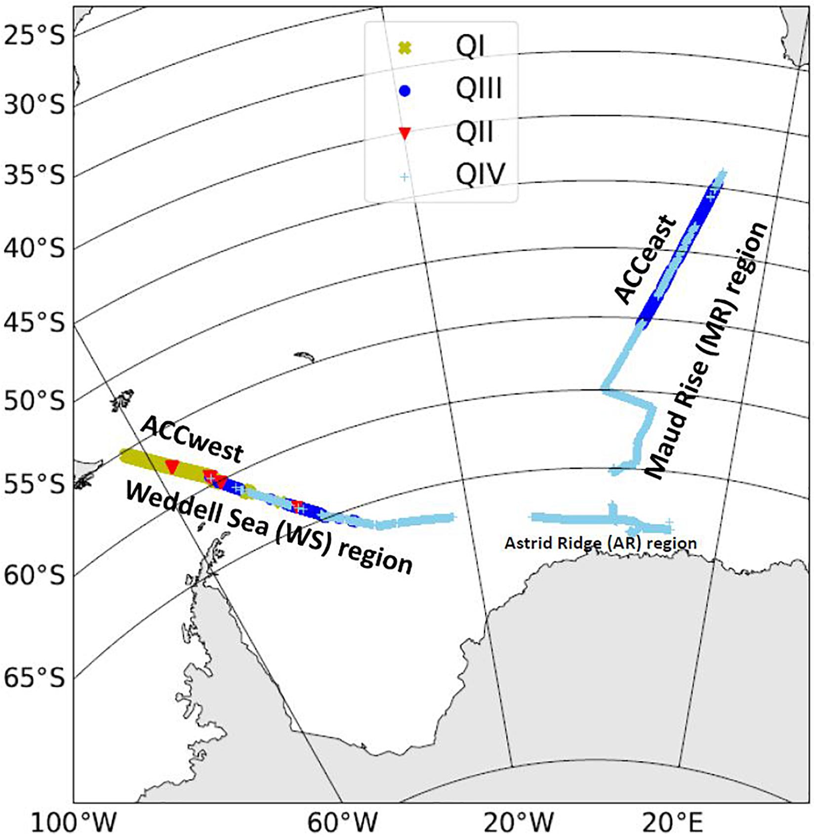
Figure 6. The spatial distribution of observations in the quadrants from the correlation model. Yellow = observations in the QI, Red = observations in QII, Deep blue = observations in QIII, and Sky blue = observations in QIV.

FIGURE 7

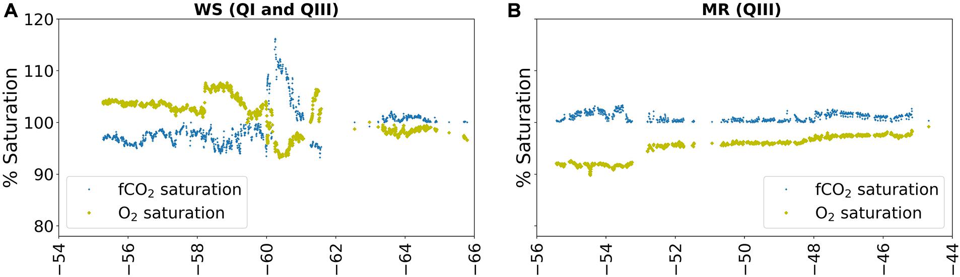
Figure 7. Spatial distribution of the fCO₂sat/O₂sat correlations for the case waters in QI and QIII. (A) WS region and (B) MR region.

For the QIII case waters in the MR region found in the ACCeast (the northern extent) in the eastern sector of the study transect (Figure 6, deep blue), the correlation value is −0.27, p < 0.001 (Figures 5C,III). The fCO₂sat/O₂sat variability for the case waters in QIII along the section of the MR is shown in Figure 7B. Although the positive AOU values in Figure 3I along this section generally indicates the respiration/remineralization process derived for the QIII case waters as shown by the fCO₂sat/O₂sat distribution (Figure 7B), the correlation values indicate no clear correlation between fCO₂sat and O₂sat for the process in this region. South of 54°S, the higher SST (Figure 3C) with increasing O₂sat (Figure 7B) is indicative of the interplay of temperature with the respiration/remineralization process. Moreover, this effect of temperature is not observed correspondingly on the fCO₂sat as the supersaturated fCO₂ was slightly above saturation level and almost constant while the undersaturated O₂ was increasing further north (Figure 7B). It is therefore deduced that temperature and photosynthesis (seen in the variation of chl-a along the section (Figure 3I), as well as respiration/remineralization processes, combine to drive the observed fCO₂sat/O₂sat variability in QIII for this region.

The overall mechanism above shows that the undersaturation and supersaturation of fCO₂sat each in QI and QIII case waters were generally driven by photosynthesis and respiration/remineralization and upwelling, respectively as derived for the quadrants. However, along the ACCeast on the MR section, the influence of temperature on the spatial distributions of fCO₂sat/O₂sat affected the fCO₂sat/O₂sat correlation in the ACC.

Surface Water Property–Property Relationship With fCO₂sat/O₂sat Correlations for Case Waters QII and QIV

The dominating process derived for the case waters QII (Figure 6, red) and QIV (Figure 6, sky blue) is the effect of temperature on the variability of fCO₂sat/O₂sat. These case waters (QII and QIV) were found in parts of the WS region while the waters of AR were completely distributed in the QIV. Waters along the southern extent and some parts of the ACCeast in the MR region were also observed as QIV case waters (Figure 6, sky blue).

The sections of the WS transect distributed in QIV were located south of 60°S in the Weddell gyre region (Figure 6, sky blue), with a considerably smaller section between 58 and 60°S (in the ACCwest) in the QII (Figure 6, red). A significant but weakly positive correlation of 0.33, p < 0.001 between fCO₂sat and O₂sat with a slope of 0.1 (Figures 5A,II,IV) was observed, indicating a weak effect of temperature on the fCO₂sat/O₂sat relationship. The low fCO₂sat/O₂sat correlation could be attributed to the near-saturation level of the supposed undersaturated fCO₂ and O₂ for most of the observations (Figure 8A), and the process vector (green regression line, Figure 5A) not passing through QII. As very few observations are in QII, this could indicate that the influence of temperature on the supersaturation of fCO₂sat and O₂sat in the QII is small. Figure 8A shows fCO₂sat/O₂sat variability for the case waters in QIV and the few observations for QII along the WS region. The cooling effect of temperature is expected as the dominant driver in QIV. However, the upwelling of rich-CO₂ indicated by the higher SSS values between 61 and 64°S and at 67°S (Figure 3A) potentially influence the fCO₂sat in Figure 8A and enhance fCO₂ to near-saturation level. Similarly, the near saturation of O₂sat (Figure 8A) could also potentially be the influence of photosynthesis along the same section (Figure 3G) enhancing the saturation of O₂. This is particularly clear around 67°S where O₂sat was enhanced with fCO₂sat greatly reduced (Figure 8A). Furthermore, the positive values of AOU, albeit low (< 20 μmol kg^–1; Figure 3G), indicate the influence of respiration/remineralization. Therefore the interplay between upwelling and respiration/remineralization and primary production (photosynthesis) enhanced the saturations of fCO₂sat and O₂sat for most of the observation for QIV in the WS. This indicates a more complex dynamic in the processes driving the observed fCO₂sat/O₂sat variability than the simplified representation of the cooling effect of temperature for the observations distributed in QIV.

FIGURE 8

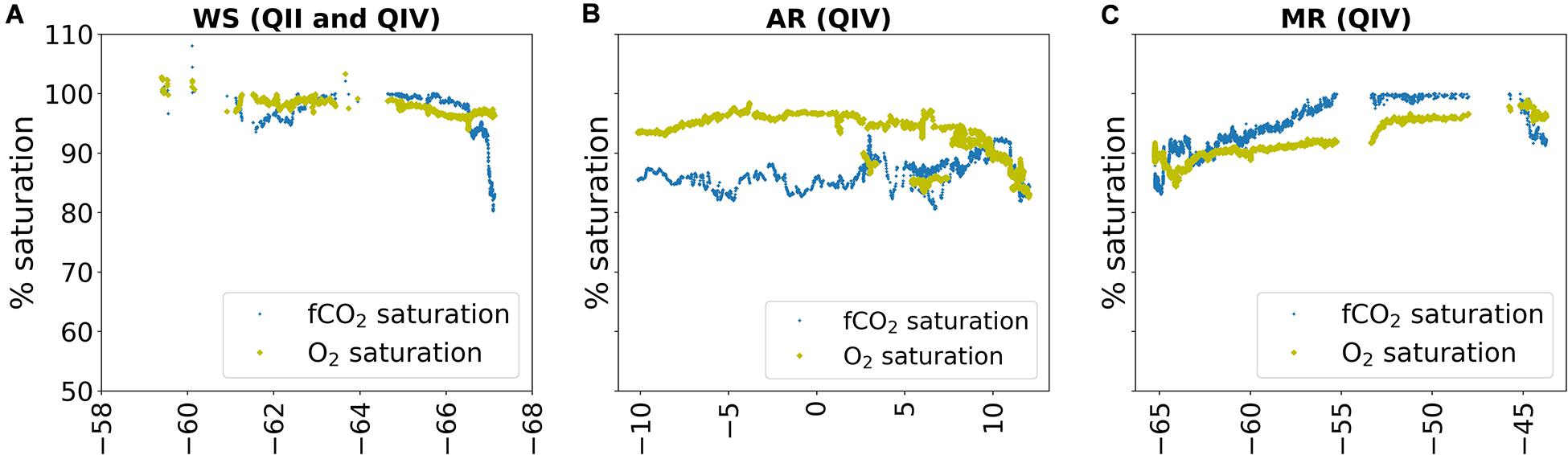
Figure 8. Spatial distribution of the fCO₂sat/O₂sat correlations for the case waters in QII and QIV. (A) WS region, (B) AR region, and (C) MR region.

The entire distribution of observations in the AR region are in the QIV (Figure 6, sky blue). The intricate interplay of different processes driving the relationship of fCO₂sat and O₂sat in the QIV is also observed in the AR region. An unexpectedly weak negative correlation of −0.19 (p < 0.001) was estimated (Figure 5B) instead of the positive correlation expected for the fCO₂sat/O₂sat relationship in QIV. Visualizing the distribution of the observations in the quadrant indicates two data populations: one, a positive correlation for fCO₂sat and O₂sat on the lower part and secondly, a negative correlation for the upper part of the distribution (Figure 5B). Figure 8B, shows the variability of fCO₂sat/O₂sat for the case waters in QIV along the AR transect. Longitudinal distributions of each of the two visualized groups (Figure 9) reveals the effect of temperature (the positive correlation) on the fCO₂sat/O₂sat at the east of 9°E, between 5 and 8°E, and at 3°E for the first group (Figures 9A,C). This is observed along the sections as both fCO₂sat and O₂sat decrease (Figure 8B) with decreasing SST and SSS (Figure 3B) which becomes significant at the east of 9°E. This could indicate cooling and freshening of the surface waters from glacial and sea-ice melt near the continent which decreases the fCO₂ and O₂ saturations (Klinck, 1998; Ohshima et al., 1998Dierssen et al., 2002; Carrillo et al., 2004). On the other hand, the longitudinal extent of the second data population distribution shows the effect of photosynthesis (negative correlation) across the whole region west of 10°E (Figure 9B,D). This corresponds with the variable chl-a concentrations associated with the fCO₂/chl-a relationship for photosynthesis along the region (see section “AR region”) and Figure 3H. The variable photosynthetic process could potentially be related to the patchy plankton blooms characteristics of Antarctic coastal waters (Carrillo et al., 2004). Furthermore, the increasing positive values of AOU along the region in the east of 9°E (Figure 3H) indicate also the influence of respiration/remineralization on the fCO₂sat/O₂sat relationship. Thus, the interplay of photosynthesis and respiration/upwelling combined with the cooling effect of temperature influence the undersaturation of fCO₂ and O₂ for AR in the QIV. This highlights the complex interaction between physical-chemical and biological processes setting the balance in the sea-air CO₂ in the Southern Ocean (Marinov et al., 2006; Henley et al., 2020).

FIGURE 9

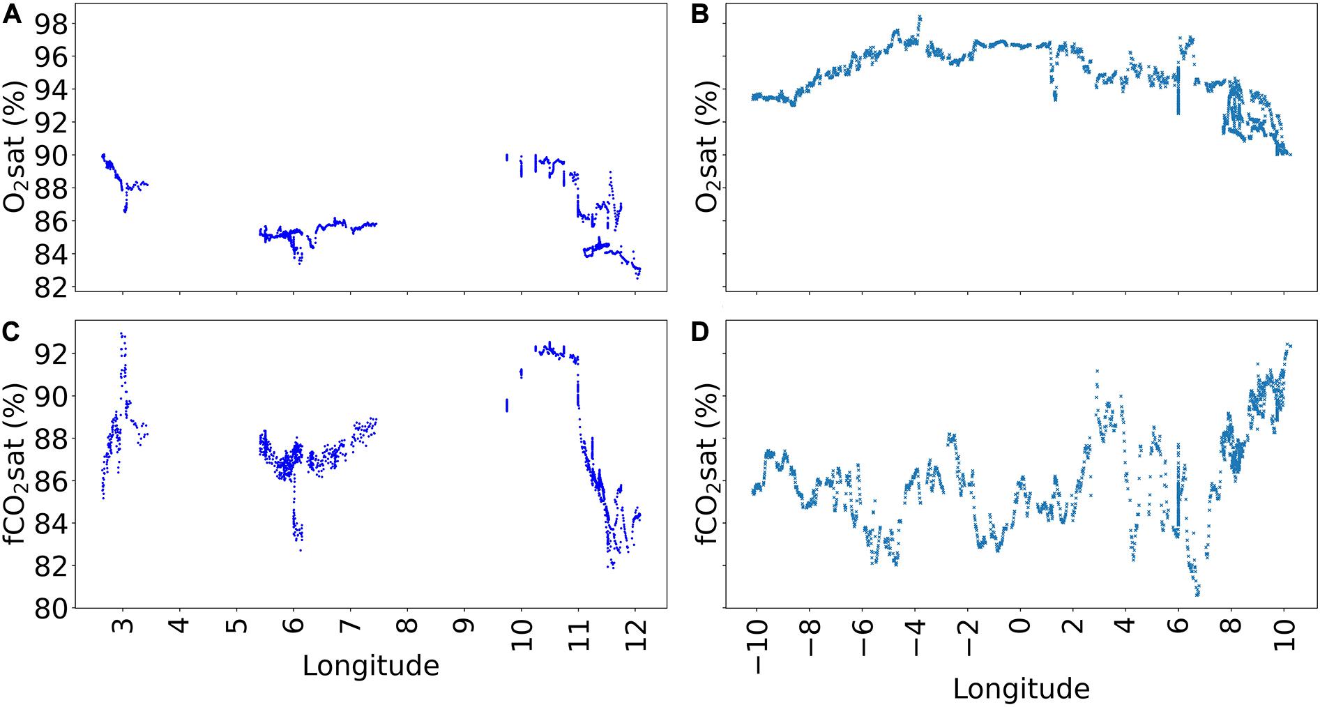
Figure 9. Longitudinal distributions of the two data populations visualized in the QIV quadrant for the AR region in Figure 5B. (A,C) Distributions of O₂sat and fCO₂sat, respectively for the positive correlation data population. (B,D) Distributions of O₂sat and fCO₂sat, respectively for the negative correlation data population.

Finally, the distribution of observations in QIV for the MR region was located between 43 and 66°S (Figure 6, sky blue) in the eastern sector of the transect. The significant positive correlation between fCO₂sat and O₂sat (0.63, p < 0.001; Figures 5C,IV) indicates the dominance of the temperature effect in QIV. The fCO₂sat/O₂sat variability for the case waters in QIV along the MR transect is presented in Figure 8C. Despite the high positive correlation value of 0.63, indicative of temperature dominated influence, respiration/remineralization process (positive values of AOU, Figure 3I) and photosynthesis (Figure 3I) also contribute to the observed CO₂/O₂ saturation states. In the northern reaches of the MR transect near the STF and the subtropical oligotrophic waters, the undersaturation of fCO₂sat and O₂sat (Figures 3C,C) indicated the influence of other processes (see Section “Regional Drivers of FCO₂”) with the surface water properties of the controlling variables defined in this study.

Given the above, it can be said that the cooling effect of temperature derived for QIV was not spatially determined except in the part of the colder and fresher waters of the Antarctic coast. The complex interplay between temperature, photosynthesis, and respiration influences the undersaturation of fCO₂sat and enhances O₂sat saturation for the Antarctic coastal waters in the QIV. Equally, upwelling-induced primary production offset the fCO₂sat for the other observations in the QIV. The sparse distribution of the observations in the QII will not allow a reliable interpretation of the observed process.

Conclusion

This study investigates the drivers of variability for fCO₂ssw and estimates the FCO₂ during autumn in the Atlantic sector of the Southern Ocean, spanning across the Weddell gyre and ACC. The net CO₂ flux to/from the atmosphere is driven by the concentration gradient between the atmosphere and the ocean and agitated by the windspeed. During the period of occupation of the Southern Ocean for this study, the whole region along the study transect acted as a net CO₂ sink for atmospheric CO₂ with an average FCO₂ of −6.2 (± 8) mmol m^–2 d^–1. The highest net uptake was observed for the Astrid Ridge region near the Antarctic continent, mainly driven by elevated biological productivity. Using fCO₂sat/O₂sat correlations, the underway-surface observations were partitioned into four quadrants, driven predominantly by (I) photosynthesis, (II) warming, (III) respiration/remineralisation, and upwelling, and (IV) cooling. Describing the spatial distributions of the fCO₂sat/O₂sat correlations for the quadrants relative to the surface water properties of controlling variables (chl-a, AOU, SST, and SSS) shows the complex interplay of the different processes driving the fCO₂ssw distributions. Overall, the observations illustrated the complex interaction between physical-chemical and biological processes setting the balance in the sea-air CO₂ flux in the Southern Ocean and explains the variation in the sea surface CO₂. For instance, the upwelling of CO₂-rich waters is offset by CO₂ uptake through photosynthesis as observed in the MR and WS region.

Finally, this work contributes to increasing the spatial and temporal coverage of observational fCO₂ data with surface layer properties in the Weddell gyre and Antarctic coastal area, given the importance of the region to the Southern Ocean’s role in the global ocean CO₂ uptake.

Data Availability Statement

The datasets used for this study are available at the Norwegian Polar Institute Data Center (NPDC) at the following website https://doi.org/10.21334/npolar.2020.cc4bfb5f and in the Surface Ocean CO₂ Atlas (SOCAT).

Author Contributions

AF, MC, and AR conceptualized the project. AF and MC collected the data and contributed specialist knowledge toward constructing and finalizing the manuscript. MO did the data analysis, interpretation, and compiled the manuscript. AR and WJ as the graduate adviser of MO also contributed specialist knowledge towards constructing and finalizing the manuscript. All authors contributed to the manuscript revisions, read, and approved the submitted version.

Conflict of Interest

The authors declare that the research was conducted in the absence of any commercial or financial relationships that could be construed as a potential conflict of interest.

Funding

The study was funded by the Research Council of Norway (RCN) project number 288370 and National Research Foundation, South Africa (Grant UID 118715) for the SANOCEAN Norway-South Africa collaboration project “Southern Ocean phytoplankton community characteristics, primary production, CO₂ flux and the effects of climate change (SOPHY-CO2).” Ph.D. bursary to MO was provided through NRF SANAP (Grant UID 110715) grant to AR and by Tertiary Education Trust Fund (TETFund) Nigeria. AF and MC were partly funded by the Fram Centre flagship research program “Ocean acidification and ecosystem effects in Northern waters” at the FRAM—High North Research Centre for Climate and the Environment. The Southern Ocean Ecosystem cruise with RV Kronprins Haakon was arranged by the Norwegian Polar Institute, with additional financial support from the Norwegian Ministry of Foreign Affairs. Measurements and data quality control were partly funded by the Integrated Carbon Observing System (ICOS).

Acknowledgments

The authors are thankful to the captain and crew on RV Kronprins Haakon. We also thank Tommy Ryan-Keogh of Southern Ocean Carbon and Climate Observatory (SOCCO) CSIR, South Africa, and Asmita Sing (Ph.D. candidate of SOCCO) affiliated to Stellenbosch University, South Africa for the chl-a underway data and Ylva Ericson at the Norwegian Polar Institute for support regarding CO₂-data reduction. The many researchers and funding agencies responsible for the collection of data and quality control are thanked for their contributions to SOCAT. The Surface Ocean CO₂ Atlas (SOCAT) is an international effort, endorsed by the International Ocean Carbon Coordination Project (IOCCP), the Surface Ocean Lower Atmosphere Study (SOLAS), and the Integrated Marine Biosphere Research (IMBeR) program, to deliver a uniformly quality-controlled surface ocean CO₂ database.

Supplementary Material

The Supplementary Material for this article can be found online at: https://www.frontiersin.org/articles/10.3389/fmars.2020.614263/full#supplementary-material

References

Arrigo, K. R., and Van Dijken, G. L. (2003). Phytoplankton dynamics within 37 Antarctic coastal polynya system. J. Geophys. Res. 108:3271. doi: 10.1029/2002JC001739

CrossRef Full Text | Google Scholar

Arrigo, K. R., van Dijken, G. L., and Bushinsky, S. (2008). Primary production in the Southern Ocean, 1997–2006. J. Geophys. Res. 113:C08004. doi: 10.1029/2007JC004551

CrossRef Full Text | Google Scholar

Atkinson, A., Whitehouse, M. J., Priddle, J., Cripps, G. C., Ward, P., and Brandon, M. A. (2001). South Georgia, Antarctica: a productive, cold water, pelagic ecosystem. Mar. Ecol. Prog. Ser. 216, 279–308. doi: 10.3354/meps216279

CrossRef Full Text | Google Scholar

Bakker, D. C. E., Alin, S. R., Bates, N. R., Becker, M., Castano-Primo, R., Cosca, C., et al. (2020). Surface Ocean CO2 Atlas Database Version 2020 (SOCATv2020) (NCEI Accession 0210711). [1999-2019]. Washington, DC: NOAA.

Google Scholar

Bakker, D. C. E., de Baar, H. J. W., and Bathmann, U. V. (1997). Changes of carbon dioxide in surface-waters during spring in the Southern Ocean. Deep Sea Res. II 4491–128. doi: 10.1016/s0967-0645(96)00075-6

CrossRef Full Text | Google Scholar

Bakker, D. C. E., Hoppema, M., Schröder, M., Geibert, W., and De Baar, H. J. W. (2008). A rapid transition from ice covered CO2-rich waters to a biologically mediated CO2 sink in the eastern Weddell Gyre. Biogeosciences 5, 1373–1386. doi: 10.5194/bg-5-1373-2008

CrossRef Full Text | Google Scholar

Bakker, D. C. E., Pfeil, B., Landa, C. S., Metzl, N., O’Brien, K. M., Olsen, A., et al. (2016). A multi-decade record of high-quality fCO2 data in version 3 of the Surface Ocean CO2 Atlas (SOCAT). Earth Syst. Sci. Data 8, 383–413. doi: 10.5194/essd-8-383-2016

CrossRef Full Text | Google Scholar

Benson, B. B., and Krause, D. (1984). The concentration and isotopic fractionation of oxygen dissolved in freshwater and seawater in equilibrium with the atmosphere. Limnol. Oceanogr. 29, 620–632. doi: 10.4319/lo.1984.29.3.0620

CrossRef Full Text | Google Scholar

Broecker, W. S., and Peng, T. H. (1983). Tracers in the Sea. Lamont-Doherty Geological Observatory. New York, NY: Columbia University.

Google Scholar

Brown, P. J., Jullion, L., Landschützer, P., and Bakker, D. C. E. (2015). Carbon dynamics of the Weddell Gyre, Southern Ocean. Glob. Biogeochem. Cycl. 29, 288–306. doi: 10.1002/2014GB005006

CrossRef Full Text | Google Scholar

Brown, P. J., Meredith, M. P., Jullion, L., Naveira Garabato, A., Torres-Valdes, S., Holland, P., et al. (2014). Freshwater fluxes in the Weddell Gyre: Results from δ18O. Philos. Trans. Royal Soc. A. 372:20130298. doi: 10.1098/rsta.2013.0298

PubMed Abstract | CrossRef Full Text | Google Scholar

Bushinsky, S. M., Landschützer, P., Rödenbeck, C., Gray, A. R., Baker, D., Mazloff, M. R., et al. (2019). Reassessing Southern Ocean air-sea CO2 flux estimates with the addition of biogeochemical float observations. Glob. Biogeochem. Cycl. 33, 1370–1388. doi: 10.1029/2019GB006176

PubMed Abstract | CrossRef Full Text | Google Scholar

Cape, M. R., Vernet, M., Kahru, M., and Spreen, G. (2014). Polynya dynamics drive primary production in the Larsen A and B embayments following ice shelf collapse. J. Geophys. Res. Oceans. 119, 572–594. doi: 10.1002/2013JC009441

CrossRef Full Text | Google Scholar

Carrillo, C. J., Smith, R. C., and Karl, D. M. (2004). Processes regulating oxygen and carbon dioxide in surface waters west of the antarctic Peninsula. Mar. Chem. 84, 161–179. doi: 10.1016/j.marchem.2003.07.004

CrossRef Full Text | Google Scholar

Chen, L., Xu, S., Gao, Z., Chen, H., Zhang, Y., Zhan, J., et al. (2011). Estimation of Monthly Air-Sea CO2 Flux in the Southern Atlantic and Indian Ocean Using in-situ and Remotely Sensed Data. Rem. Sens. Environ. 115. 1935–1941. doi: 10.1016/j.rse.2011.03.016

CrossRef Full Text | Google Scholar

Chierici, M., Signorini, S. R., Mattsdotter-Björk, M., Fransson, A., and Olsen, A. (2012). Surface water fCO2 algorithms for the high-latitude Pacific sector of the Southern Ocean. Remote Sens. Environ. 119, 184–196. doi: 10.1016/j.rse.2011.12.020

CrossRef Full Text | Google Scholar

Chierici, M, Fransson, A, Turner, D, Pakhomov, E. A., and Froneman, P. W. (2004). Variability in pH, fCO2, oxygen, and flux of CO2 in the surface water along a transect in the Atlantic sector of the Southern Ocean. Deep Sea Res. II. 51, 2773–2787. doi: 10.1016/j.dsr2.2001.03.002

CrossRef Full Text | Google Scholar

Deacon, G. E. R. (1982). Physical and biological zonation in the Southern Ocean. Deep Sea Res. 29, 1–15. doi: 10.1016/0198-0149(82)90058-9

CrossRef Full Text | Google Scholar

Deacon, G. E. R. (1979). The Weddell Gyre. Deep Sea Res. 26, 981–995.

Google Scholar

Dieckmann, G. S., Nehrke, G., Papadimitriou, S., Göttlicher, J., Steininger, R., Kennedy, H., et al. (2008). Calcium carbonate as ikaite crystals in Antarctic sea ice. Geophys. Res. Lett. 35, 35–37. doi: 10.1029/2008GL033540

CrossRef Full Text | Google Scholar

Dierssen, H. M., Smith, R. C., and Vernet, M. (2002). Glacial meltwater dynamics in coastal waters west of the Antarctic peninsula. PNAS 99, 1790–1795 doi: 10.1073/pnas.032206999

PubMed Abstract | CrossRef Full Text | Google Scholar

Fahrbach, E. (2006). The Expedition ANTARKTIS-XXII/3 of the Research Vessel “Polarstern” in 2005. Rep. Ber. Polar Meeresforsch. 533, 1–246. doi: 10.1002/352760412x.ch1

CrossRef Full Text | Google Scholar

Fransson, A., Chierici, M., Yager, P., and Smith, W. O. (2011). Antarctic sea ice carbon dioxide system and controls. J. Geophys. Res. 116:C12035, doi: 10.1029/2010JC006844

CrossRef Full Text | Google Scholar

Fransson, A, Chierici, M, Anderson, L. G., and David, R. (2004). Transformation of carbon and oxygen in the surface layer of the eastern Atlantic sector of the Southern Ocean. Deep Sea Res. II. 51, 2757–2772.

Google Scholar

Freeman, N. M. (2017). Physical and Biogeochemical Features of the Southern Ocean: Their Variability and Change Over the Recent Past and Coming Century. PhD Thesis. Boulder: University of Colorado

Google Scholar

Frölicher, T. L., Sarmiento, J. L., Paynter, D. J., Dunne, J. P., Krasting, J. P., and Winton, M. (2015). Dominance of the Southern Ocean in anthropogenic carbon and heat uptake in CMIP5 models. J. Clim. 28:2. doi: 10.1175/JCLI-D-14-00117.1

CrossRef Full Text | Google Scholar

Froneman, P. W., Pakhomov, E. A., and Balarin, M. G. (2004). Size fractionated phytoplankton biomass, production and biogenic carbon flux in the eastern Atlantic sector of the Southern Ocean in late austral summer 1997-1998. Deep Sea Res. II. 51, 2715–2729. doi: 10.1016/j.dsr2.2002.09.001

CrossRef Full Text | Google Scholar

Garcia, H. E., and Gordon, L. I. (1992). Oxygen solubility in seawater: better fitting equations. Am. Soc. Limnol. Oceanogr. Inc. 37, 1307–1312. doi: 10.4319/lo.1992.37.6.1307

CrossRef Full Text | Google Scholar

Garcia, H. E., Locarnini, R. A., Boyer, T. P., Antonov, J. I., Mishonov, A. V., Baranova, O. K., et al. (2013). WORLD OCEAN ATLAS 2013 Vol 3, Dissolved Oxygen, Apparent Oxygen Utilization, and Oxygen Saturation, ed S. Levitus, and A. Mishonov, (Washingdon, DC: NOAA).

Google Scholar

Gordon, A. L., and B. A., Huber (1990). Southern Ocean winter mixed layer. J. Geophys. Res. 95, 655–672. doi: 10.1029/JC095iC07p11655.

CrossRef Full Text | Google Scholar

Grant, S., Constable, A., Raymond, B., and Doust, S. (2006). Bioregionalisation of the Southern Ocean: Report of experts’ workshop. Hobart: WWF-Australia and ACE CRC.

Google Scholar

Gregor, L., Kok, S., and Monteiro, P. M. S. (2018). Interannual drivers of the seasonal cycle of CO2 in the Southern Ocean. Biogeosciences 15, 2361–2378. doi: 10.5194/bg-15-2361-2018

CrossRef Full Text | Google Scholar

Gruber, N., Gloor, M., Mikaloff, F. S. E., Doney, S. C., Dutkiewicz, S., Michael, J., et al. (2009). Oceanic sources, sinks, and transport of atmospheric CO2. Glob. Biogeochem. Cycl. 23:GB1005. doi: 10.1029/2008GB003349

CrossRef Full Text | Google Scholar

Hauck, J., Hoppema, M., Bellerby, R. G. J., Volker, C., and Wolf-Gladrow, D. (2010). Data-based estimation of anthropogenic carbon and acidification in the Weddell Sea on a decadal timescale. J. Geophys. Res. 115:C03004. doi: 10.1029/2009JC005479

CrossRef Full Text | Google Scholar

Hellmer, H. H., Rhein, M., Heinemann, G., Abalichin, J., Abouchami, W., Baars, O., et al. (2016). Meteorology and oceanography of the Atlantic sector of the Southern Ocean—A review of German achievements from the last decade. Ocean Dyn. 66, 1379–1413. doi: 10.1007/s10236-016-0988-1

CrossRef Full Text | Google Scholar

Henley, S. F, Cavan, E. L, Fawcett, S. E, Kerr, R, Monteiro, T, Sherrell, R. M, et al. (2020). Changing Biogeochemistry of the Southern Ocean and Its Ecosystem Implications. Front. Mar. Sci. 7:581. doi: 10.3389/fmars.2020.00581

CrossRef Full Text | Google Scholar

Heywood, K. J., Naveira Garabato, A. C., and Stevens, D. P. (2002). High mixing rates in the abyssal Southern Ocean. Nature 415, 1011–1015.

Google Scholar

Heywood, K. J., Naveira Garabato, A. C., Stevens, D. P., and Muench, R. D. (2004). On the fate of the Antarctic Slope Front and the origin of the Weddell Front. J. Geophys. Res. C 109, 06013–06021.

Google Scholar

Holm-Hansen, O., Kahru, M., and Hewes, C. D. (2005). Deep Chlorophyll a Maxima (DCMs) in Pelagic Antarctic Waters. II. Relation to Bathymetric Features and Dissolved Iron Concentrations. Mar. Ecol. Prog. Ser. 297, 71–81. doi: 10.3354/meps297071

CrossRef Full Text | Google Scholar

Holm-Hansen, O., and Riemann, B. (1978). Chlorophyll a determination: Improvements in methodology. Oikos 30, 438–447.

Google Scholar

Hoppema, M. (2004). Weddell Sea is a globally significant contributor to deep-sea sequestration of natural carbon dioxide. Deep Sea Res. 51, 1169–1177. doi: 10.1016/j.dsr.2004.02.011

CrossRef Full Text | Google Scholar

Hoppema, M., Fahrbach, E., Schröder, M., Wisotzki, A., and de Baar, H. J. W. (1995). Winter-summer differences of carbon dioxide and oxygen in the Weddell Sea surface layer. Mar. Chem. 51, 177–192. doi: 10.1016/0304-4203(95)00065-8

CrossRef Full Text | Google Scholar

Hoppema, M., Fahrbach, E., Stoll, M. H. C., and De Baar, H. J. W. (1999). Annual uptake of atmospheric CO2 by the Weddell Sea derived from a surface layer balance, including estimations of entrainment and new production. J. Mar. Syst. 19, 219–233. doi: 10.1016/s0924-7963(98)00091-8

CrossRef Full Text | Google Scholar

Hoppema, M., Stoll, M. H. C., and De Baar, H. J. W. (2000). CO2 in the Weddell Gyre and Antarctic Circumpolar Current : Austral Autumn and Early Winter. Mar. Chem. 72, 203–220.

Google Scholar

Ito, T., Woloszyn, M., and Mazloff, M. (2010). Anthropogenic carbon dioxide transport in the Southern Ocean driven by Ekman flow. Nature 463, 80–83. doi: 10.1038/nature086687

CrossRef Full Text | Google Scholar

Kauko, H. M. T., Hattermann, T. J., Ryan-Keogh, A., Singh, L., de Steur, A., Fransson, M, et al. (in review) Phenology and environmental control of phytoplankton blooms in the Kong Håkon VII Hav in the Southern Ocean. Front. Mar. Sci..

Google Scholar

Kheshgi, H. S. (2004). Ocean sink duration under stabilization of atmospheric CO2: A 1, 000-year timescale. Geohys. Res. Lett. 31:L20204. doi: 10.1029/2004GL020612

CrossRef Full Text | Google Scholar

Klinck, J. M. (1998). Heat and salt changes on the continental shelf west of the Antarctic Peninsula between January 1993 and January 1994. J. Geophys. Res. 103, 7617–7636. doi: 10.1029/98jc00369

CrossRef Full Text | Google Scholar

Lencina-Avila, J. M., Ito, R. G., Garcia, C. A. E., and Tavano, V. M. (2016). Sea-air carbon dioxide fluxes along 35°S in the South Atlantic Ocean. Deep Sea Res. Pt. I Oceanogr. Res. Pap. 115, 175–187. doi: 10.1016/j.dsr.2016.06.004

CrossRef Full Text | Google Scholar

Lenton, A., Tilbrook, B., Law, R. M., Bakker, D., Doney, S. C., Gruber, N., et al. (2013). Sea-air CO2 fluxes in the Southern Ocean for the period 1990-2009. Biogeosciences. 10, 4037–4054. doi: 10.5194/bg-10-4037-2013

CrossRef Full Text | Google Scholar

Long, M. C., Lindsay, K., Peacock, S., Moore, J. K., and Doney, S. C. (2013). Twentieth-century oceanic carbon uptake and storage in CESM1 (BGC). J. Clim. 26, 6775–6800.

Google Scholar

Marinov, I., Gnanadesikan, A., Toggweiler, J. R., and Sarmiento, J. L. (2006). The southern ocean biogeochemical divide. Nature 441, 964–967. doi: 10.1038/nature04883

PubMed Abstract | CrossRef Full Text | Google Scholar

Mattsdotter-Björk, M., Fransson, A., Torstensson, A., and Chierici, M. (2014). Ocean acidification state in western Antarctic surface waters: Controls and interannual variability. Biogeosciences 11, 57–73. doi: 10.5194/bg-11-57-2014

CrossRef Full Text | Google Scholar

McKinley, G. A., Fay, A. R., Lovenduski Nicole, S., and Pilcher Darren, J. (2017). Natural Variability and Anthropogenic Trends in the Ocean Carbon Sink. Annu. Rev. Mar. Sci. 9, 1.26–9.26. doi: 10.1146/annurev-marine-010816-060529

PubMed Abstract | CrossRef Full Text | Google Scholar

Metzl, N., Brunet, C., Jabaud-Jan, A., Poisson, A., and Schauer, B. (2006). Summer and winter air–sea CO2 fluxes in the Southern Ocean. Deep Sea Res. I 53, 1548–1563. doi: 10.1016/j.dsr.2006.07.006

CrossRef Full Text | Google Scholar

Mongwe, N. P., Chang, N., and Monteiro, P. M. S. (2016). The seasonal cycle as a mode to diagnose biases in modelled CO2 fluxes in the Southern Ocean. Ocean Model. 106, 90–103. doi: 10.1016/j.ocemod.2016.09.006

CrossRef Full Text | Google Scholar

Monteiro, P. M. S., Gregor, L., Levy‘, M., Maenner, S., Sabine, C. L., and Swart, S. (2015). Intraseasonal variability linked to sampling alias in air-sea CO2 fluxes in the Southern Ocean. Geophys. Res. Lett. 42, 8507–8514. doi: 10.1002/2015GL066009

CrossRef Full Text | Google Scholar

Monteiro, P. M. S., Schuster, U., Hood, M., Lenton, A., Metzl, N., Olsen, A., et al. (2010). “A Global Sea Surface Carbon Observing System: Assessment of Changing Sea Surface CO2 and Air-Sea CO2 Fluxes,” in Proceedings of OceanObs’09: Sustained Ocean Observations and Information for Society Vol. 2, Venice. doi: 10.5270/OceanObs09.cwp.64

CrossRef Full Text | Google Scholar

Moreau, S., di Fiori, E., Schloss, I. R., Almandoz, G. O., Esteves, J. L., Paparazzo, F. E., et al. (2013). The role of phytoplankton composition and microbial community metabolism in sea-air Delta pCO2 variation in the Weddell Sea. Deep Sea Res. Pt. I. 82, 44–59. doi: 10.1016/j.dsr.2013.07.010

CrossRef Full Text | Google Scholar

Mu, L., Stammerjohn, S. E., Lowry, K. E., and Yager, P. L. (2014), Spatial variability of surface pCO2 and air-sea CO2 flux in the Amundsen Sea Polynya, Antarctica. Elem. Sci. Anthropocene. 2:000036. doi: 10.12952/journal.elementa.000036

CrossRef Full Text | Google Scholar

Munro, D. R., Lovenduski, N. S., Stephens, B. B., Newberger, T., Arrigo, K. R., Takahashi, T., et al. (2015). Estimates of net community production in the Southern Ocean determined from time-series observations (2002–2011) of nutrients, dissolved inorganic carbon, and surface ocean pCO2 in Drake Passage. Deep Sea Res. Pt. II 114, 49–63. doi: 10.1016/j.dsr2.2014.12.014

CrossRef Full Text | Google Scholar

Ohshima, K. I., Yoshida, K., Shimoda, H., Wakatsuchi, M., Endoh, T., and Fukuchi, M. (1998). Relationship between the upper ocean and sea ice during the Antarctic melting season. J. Geophys. Res. 103, 7601– 7615

Google Scholar

Orsi, A. H., Whitworth, T., and Nowlin, W. D. (1995). On the meridional extent and fronts of the antarctic circumpolar current. Deep Sea Res. Part I. 42, 641–673. doi: 10.1016/0967-0637(95)00021-W

CrossRef Full Text | Google Scholar

Pierrot, D., Neill, C., Sullivan, K., Castle, R., Wanninkhof, R., Lüger, H., et al. (2009). Recommendations for autonomous underway pCO2 measuring systems and data-reduction routines. Deep Sea Res. Pt. II Top. Stud. Oceanogr. 56:8–10) 512–522. doi: 10.1016/j.dsr2.2008.12.005

CrossRef Full Text | Google Scholar

Pollard, R. T., Lucas, M. I., and Read, J. F. (2002). Physical controls on biogeochemical zonation in the Southern Ocean. Deep Sea Res. Part II Top. Stud. Oceanogr. 49, 3289–3305. doi: 10.1016/S0967-0645(02)00084-X

CrossRef Full Text | Google Scholar

Roden, N. P., Tilbrook, B., Trull, T. W., Virtue, P., and Williams, G. D. (2016). Carbon cycling dynamics in the seasonal sea-ice zone of East Antarctica. J. Geophys. Res. Oceans 121, 8749–8769.

Google Scholar

Roshan, S., and DeVries, T. (2017). Efficient dissolved organic carbon production and export in the oligotrophic ocean. Nat. Commun. 8:2036.

Google Scholar

Sabine, C. L., Feely, R. A., Gruber, N., Key, R. M., Lee, K., Bullister, J. L., et al. (2004). The oceanic sink for anthropogenic CO2. Science 305, 367–371. doi: 10.1126/science.1097403

PubMed Abstract | CrossRef Full Text | Google Scholar

Schmittner, A., Chiang, J. C. H., Hemming, S. R. (2007). “Introduction: the ocean’s meridional overturning circulation,” in Ocean Circulation: Mechanisms and Impacts- Past and Future Changes of Meridional Overturning, Vol. 173, eds. A. Schmittner, J. C. H. Chiang, and S. R. Hemming, 1–4. doi: 10.1029/173GM02

CrossRef Full Text | Google Scholar

Shadwick, E. H., Tilbrook, B., and Williams, G. D. (2014). Carbonate chemistry in the Mertz Polynya (East Antarctica): Biological and physical modification of dense water outflows and the export of anthropogenic CO2. J. Geophys. Res. Oceans 119, 1–14,Google Scholar

Sigman, D. M., and Hain, M. P. (2012). The Biological Productivity of the Ocean. Nat. Educ. Knowl. 3:21

Google Scholar

Smith, W, and Barber, D eds (2007). Polynyas: Windows to the World. Oxford: Elsevier.

Google Scholar

Stoll, MHC, de Baar HJW, Hoppema M, and Fahrbach, E. (1999). New early winter fCO2 data reveal continuous uptake of CO2 by the Weddell Sea. Tellus 679–687, doi: 10.3402/tellusb.v51i3.16460

CrossRef Full Text | Google Scholar

Strass, V. H., Leach, H., Prandke, H., Donnelly, M., Bracher, A. U., and Wolf-gladrow, D. A. (2017). The physical environmental conditions for biogeochemical differences along the Antarctic Circumpolar Current in the Atlantic Sector during late austral summer 2012. Deep Sea Res. Part II 138, 6–25. doi: 10.1016/j.dsr2.2016.05.018

CrossRef Full Text | Google Scholar

Takahashi, T., Sutherland, S. C., Chipman, D. W., Goddard, J. G., Ho, C., and Newberger, T, et al. (2014). Climatological distributions of pH, pCO2, total CO2, alkalinity, and CaCO3 saturation in the global surface ocean, and temporal changes at selected locations. Mar. Chem. 164, 95–125

Google Scholar

Takahashi, T., Sutherland, S. C., Wanninkhof, R., Sweeney, C., Feely, R. A., Chipman, D. W., et al. (2009). Climatological mean and decadal change in surface ocean pCO2, and net sea-air CO2 flux over the global oceans. Deep Sea Res. Part II Top. Stud. Oceanogr. 56, 554–577. doi: 10.1016/j.dsr2.2008.12.009

CrossRef Full Text | Google Scholar

Takahashi, T., Sweeney, C., Hales, B., Chipman, D. W., NewBerger, T., Goddard, J. G., et al. (2012). The changing carbon cycle in the Southern Ocean. Oceanography 25, 56–67. doi: 10.5670/oceanog.2011.65

CrossRef Full Text | Google Scholar

Vernet, M., Geibert, W., Hoppema, M., Brown, P. J., Haas, C., Hellmer, H. H., et al. (2019). The weddell gyre, southern ocean: present knowledge and future challenges. Rev. Geophys. 57, 1–86. doi: 10.1029/2018RG000604

CrossRef Full Text | Google Scholar

Wanninkhof, R. (2014). Relationship between wind speed and gas exchange over the ocean revisited. Limnol Oceanogr. Methods 12, 351–362. doi: 10.4319/lom.2014.12.351

CrossRef Full Text | Google Scholar

Wanninkhof, R., Park, G. H., Takahashi, T., Sweeney, C., Feely, R., Bullister, J. L., et al. (2013). Global ocean carbon uptake: Magnitude, variability, and trends. Biogeosciences 10, 1983–2000 doi: 10.5194/bg-10-1983-2013

CrossRef Full Text | Google Scholar

Weiss, R. F. (1974). Carbon Dioxide in Water and Seawater: The Solubility of Non-ideal Gas. Mar. Chem. 2, 203–215. doi: 10.1016/0304-4203(74)90015-2

CrossRef Full Text | Google Scholar