Low-Cost, Computer Vision-Based, Prebloom Cluster Count Prediction in Vineyards

Introduction

Despite advances in vineyard management techniques, one of the most challenging aspects in viticulture involves accurate estimation of grapevine yield. Yield estimates are used prior to harvest to allocate resources such as labor, tank space, and packaging, as well as to predict revenue. Progress in yield estimation methods—either through cost reduction or increased precision—could have a significant impact on the economic well-being of the viticulture industry. For example, after a drought in 2016, anecdotal reports from grape growers in the Finger Lakes region of NY in 2017 suggested most yield estimates only accounted for approximately two thirds of the actual yield at harvest.

Most techniques for yield estimation are manual and/or destructive (Atzberger, 2013; Ma et al., 2016), and involve counting clusters and assessing average cluster weight. One such method, called the Largest Cluster Weight Method, is simply multiplying an estimate of the number of clusters in the vineyard by the historic average weight of a single cluster. The inherent weakness of this method is that it relies on long-term averages and does not consider the often dramatic annual fluctuations in environmental conditions that impact the number of clusters and average cluster weight. Other methods, such as the Lag-Phase Method and the Growing Degree Day Method (Dami and Sabbatini, 2011), attempt to predict the final berry weight based on early-stage cluster weight and environmental conditions. These methods offer an alternative method only for the final berry weight estimate and provide no superior method for cluster number estimates (Dami and Sabbatini, 2011). Estimating the number of clusters in the vineyard is often accomplished by manually counting a subset of the vineyard and extrapolating the average of this subset over the size of the entire vineyard. This method is laborious and time consuming and may result in lost revenue due to inaccurate estimates. It can also be highly inaccurate for vineyards in cool climates where environmental conditions year to year result in significant variation in cluster weight and number of clusters per vine.

To automate yield prediction many researchers have turned to vision-based sensing for cluster and berry counting as well as weight estimates. Specifically, there has been significant focus on imaging vines from the side of the trellis as described in a comprehensive recent review (Seng et al., 2018). Current methods tend to rely on systems such as high precision LIDAR and RGB, stereovision, and/or near infrared cameras. Such systems can cost thousands or tens of thousands of dollars. These methods achieve reasonable success in warm climates with small vines (Rose et al., 2016; Rist et al., 2018), but in regions such as the Northeastern U.S. where grapevines are highly vigorous due to high organic matter in the soil and ample precipitation, foliage often impedes visual assessment resulting in inaccurate measurements.

In pursuit of a more accessible and effective yield estimation technique for use in cool climate vineyards, we propose to leverage standard computer vision techniques (machine learning and optical tracking) on videos captured from a comparably low-cost smartphone carried through the vineyard by a vehicle, robot, or person. The goal is to achieve more accurate cluster counts than averaging a subset of manually counted vines, while keeping the cost affordable to small vineyard owners and below alternative computer vision methods. Instead, a small subset of manually counted vines and/or previous years data is used to calibrate computer vision generated estimates from videos, offering higher accuracy than manual counting alone. Our key insight is that by deploying these techniques at the early stages of the growth cycle, between Eichhorn-Lorenz (EL) stages 12–15 (Eichhorn and Lorenz, 1977), there are significant benefits to be gained. First, early cluster counts gives the grower more time to capitalize on the yield prediction insight. Second, this phenological stage occurs before the canopy has fully closed, allowing for greater visibility of the clusters. Furthermore, different cultivars of grapes share greater visual similarities earlier in the year. As the vine develops, features that visually distinguish different cultivars become more prominent, requiring more training data and a more complex computer vision model to accommodate the visual variations among them. Lastly, during EL 12–15, the shoots are relatively short and the ends of the shoots are new growth, which has distinct visual features.

Specifically, we implement a machine learning (ML) framework, testing a variety of classifiers and trackers, and show that early clusters have a high likelihood of being detected and that their numbers correlate with final harvest data. We further use training data from videos collected by one user to count clusters in videos collected by another to show general applicability. We also explore the reliability of manual counting techniques and the challenges associated with variations between different counters, and how augmenting these counts with computer vision can improve the reliability of these cluster count estimations.

Materials and Methods

Experimental Overview

This work was undertaken at the Cornell teaching vineyard in Lansing, NY (42°34′22.32″N, 76°35′48.22″W). Mature Vitis vinifera L. grapevines with vine spacing of 6 ft × 9 ft were cane-pruned and vertically shoot-positioned according to regional practices (Wolf, 2008).

Four separate datasets were collected to investigate cluster number counting in the vineyard. The first dataset was used to evaluate yield estimates given a manually counted subset of the vineyard. For all counts collected, counters were given a handheld tally counters and instructed to count the number of shoots and clusters in each panel (composed of four vines each). In 2019, the counters were Cornell undergraduate student in the summer Cornell Orchards intern program. They were instructed to touch each shoot and cluster they counted, moving their hands through the vine to push aside foliage, increasing the visibility of the cluster. In 2019, manual counts of 70 panels (280 vines) were performed by four different counters, counting the entire set of vines twice, each count being performed by a different individual. In 2020, one manual count of 78 panels (312 vines) was performed by a single graduate student who had a strong background in viticulture and data collection.

The second dataset, collected in June 2019, measured the number of clusters per shoot. This was done by randomly selecting 400 shoots from the vineyard and counting the number of clusters on each shoot. 200 shoots were counted manually in the field, the other 200 were counted using images taken of the vine with a smartphone camera. To ensure no counting bias, equal samples were taken from the west and the east side of the rows for both datasets.

For the third dataset, four different individuals were tasked with counting the same panel, containing four Riesling vines, during the same week that the 2019 automated cluster count data was collected. They were instructed to count this single panel with the same efficiency as the rest of the dataset. The purpose of this relatively small investigation was to determine the variance in clusters counts amongst different counters.

The last dataset consisted of videos of a drive by for each panel, to be used for generating automated counts of vine features. The aim was to use these automated counts, with calibration from manual counts, to estimate the number of clusters better than a simple average of a subset of the vineyard as proposed by Pool (2001), Dami and Sabbatini (2011). To validate total yield predictions for the manual and automated counting methods, each panel was counted a second time during harvest and used as a baseline for measurement. The harvest count is considered to be the most accurate manual count for two reasons. First, every grape cluster in the vineyard must be harvested, and very few are missed, minimizing undercounting. Second, once a cluster is harvested, it is removed from the vine and placed into a bin. This eliminates the potential for double counting any cluster, minimizing over counting.

Video footage of the vines was captured in late May—early June, corresponding to EL phenological stages 12–15. These phenological stages were chosen because clusters are visible but minimally occluded by foliage, maximizing the ability to count clusters visually. Manual counts of shoots and clusters as well as video data were collected during 2019 on 78 panels (312 vines) of Riesling and during 2020 on 40 panels (160 vines) of Riesling and 30 panels (120 vines) of Pinot noir. In 2019, video data was collected with the camera and lights mounted to an ATV which was driven down the row. In 2020, video data was collected with the camera and lights being held by a person walking down the row.

Automated Counting

Automated counts were acquired through a combination of machine learning object detection and optical tracking. The videos were collected using an iPhone^® XR shooting at 240 frames per second in 1080 by 1920-pixel resolution. This frame rate allows for better visual tracking of vine features to eliminate double counting. The phone was held in a Zhiyun Smooth-Q 3-Axis Gimbal ($80) for stabilization, reducing the effects of bumpy ground and/or footsteps. The gimbal was mounted to an ATV using a tripod as shown in Figure 1. Two battery powered Neewer CN-160 LED light panels ($24), each capable of producing 900 Lux at 1 meter, were mounted above and below the phone to illuminate the vines and reduce shadows cast by the leaves. Videos were captured shortly after sunset (10 p.m.) to maintain reproducible lighting conditions, reducing the amount of training data and model complexity needed for the object detection algorithm. Nighttime also provided less windy conditions, reducing rapid movement and motion blur of clusters and shoots. An ATV (all-terrain vehicle) was driven down the row at ~1.6 km/h, taking anywhere from 2.5 to 3.5 min per row (10 panels or 40 vines).

FIGURE 1

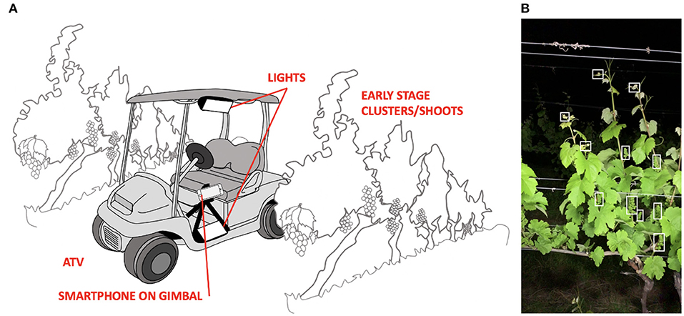
Figure 1. (A) Diagrammatic representation of setup to perform automated cluster and shoot counts in vineyards. (B) Frame from the recorded video, with example clusters highlighted in the white box.

A system overview of the counting software is given in Figure 2B. Our software framework used a Faster Region-based Convolutional Neural Network (Faster R-CNN) (Ren et al., 2016) with a ResNet50 (He et al., 2016) feature extractor for automated object detection. Detected objects were then tracked from frame to frame using a Kernelized Correlation Filter (Henriques et al., 2014) to prevent double counting. New detections were associated with previous trackers using an intersection over union metric (IOU).

FIGURE 2

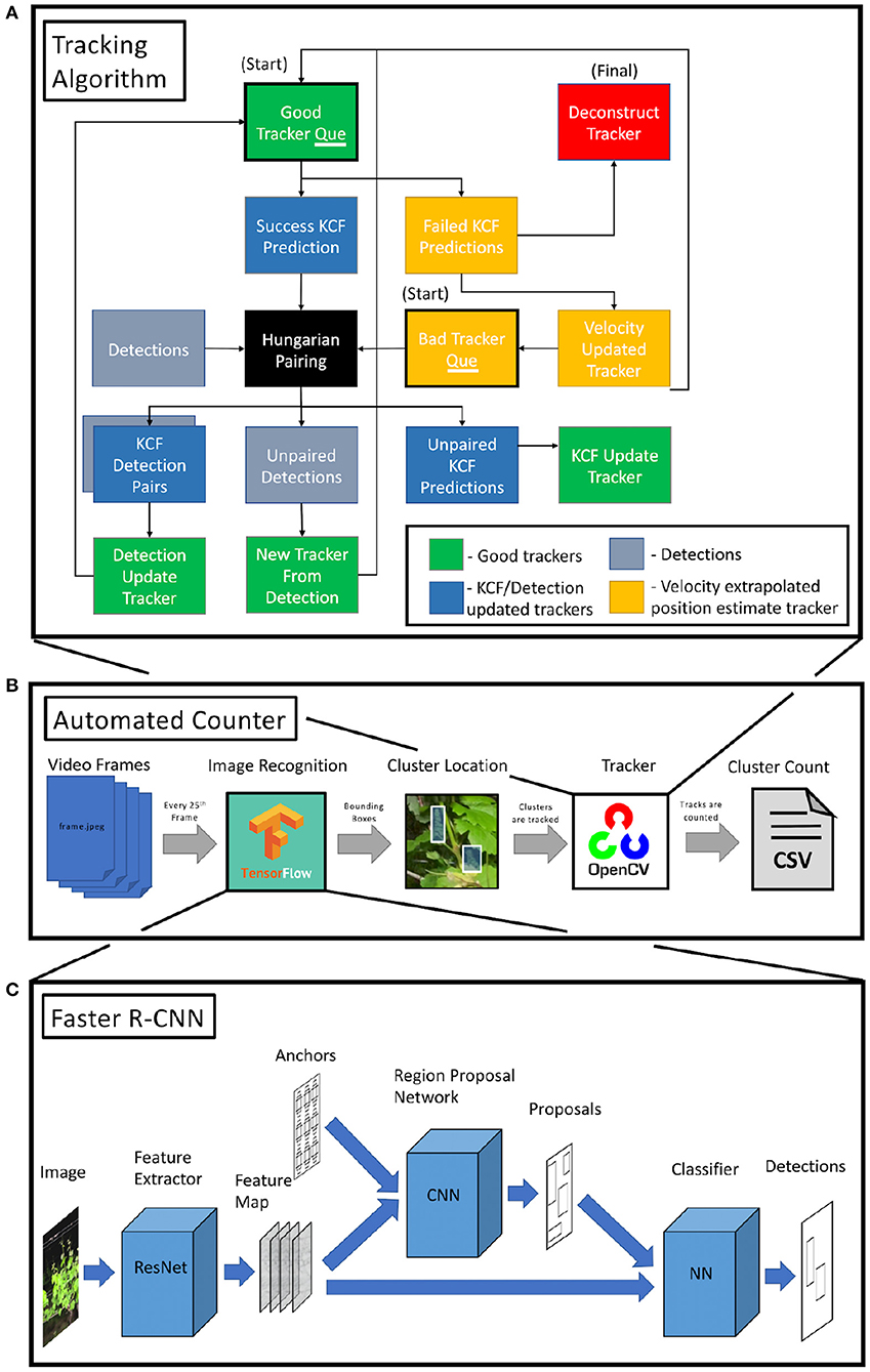
Figure 2. (A) Overview of tracking algorithm used to reduce cluster recounting. Trackers start in one of the two queues (black outline) and are updated using either KCF or, in the event that KCF fails, velocity extrapolation and are then paired with new detections. Unpaired detections are converted into trackers and reenter the queue to be processed in the subsequent frame. (B) System overview of CV software. Video frames are passed into the object detector. These detections are then passed into the tracking algorithm and tallied. (C) Overview of the Faster R-CNN. Three separate networks are used for feature extraction, object location proposal, and classification.

The Faster R-CNN was implemented using a TensorFlow¹ model which was pretrained on the COCO dataset (cocodataset.org). Using a pretrained model reduces the amount of new training data and time needed to detect clusters and shoots. The final network was trained on 611 images containing 4,580 clusters and 1,158 images containing 6,746 shoots. Performance metrics were validated on 108 images containing 829 clusters and 204 images containing 1,201 shoots. To test the transferability of the system across different years and cultivars, the network was separately trained on images collected on Riesling vines from 2019 and validated on Riesling and Pinot noir vines from 2020, however the final network was trained on images from both growing seasons. The images were labeled by two student interns and reviewed and edited by a third person to ensure quality. Image labels were generated using an open-source Python-based utility called LabelImg². Bounding boxes were selected to minimally enclose the entirety of the visible part of the grape cluster and the largest white leaf at the top of the shoot. Training the network took ~5.5 h on an 8-core Xeon workstation with a Nvidia GeForce GTX 1080; a computer that costs ~$1,500 U.S.

The Faster R-CNN is composed of three main models as shown in Figure 2C. First, high level image features are extracted using a ResNet50 feature extractor. The ResNet architecture has been proven to perform well on a variety of computer vision tasks, winning first place in the 2015 ImageNet classification, localization, and detection competitions as well as the 2015 COCO detection and segmentation competitions. These image features were then passed, in conjunction with a set of anchors, into a region proposal network (RPN). Anchors are a set of uniformly distributed bounding boxes of various size and ratio. The RPN (a fully connected CNN), uses the ResNet50 generated features to select and finetune the anchors that most closely resemble an object, generating object proposals including a bounding box and objectness score. The 256 × 256 anchors of stride 16; scale factors of 0.25, 0.5, 1, and 2; and aspect ratios of 0.5, 1, and 2. Because these anchors were used by the RPN to propose cluster and shoot locations, the anchor parameters were selected to resemble the bounding boxes in the training and validation data. This reduces the amount of learning the RPN needs to do during training. The size and shape of the grape clusters and shoots are relatively similar within the frame because the distance between the camera and the vine is relatively steady, allowing us to reduce the number of anchors and simplify the model. The features generated by the ResNet50 backbone which correspond to the object region generated by the RPN, are then passed into a traditional neural network classifier to determine the object class.

Visual trackers were used to maintain the unique identity of each cluster or shoot as it moves across the frame in the video. As shown in Figure 2A, at each new frame, new positions for each tracker are predicted using a Kernelized Correlation Filter (KCF). The KCF tracker was implemented using OpenCV³, an open-source computer vision repository. A simple Hungarian Algorithm (Kuhn, 1955) was used to pair new object detections with existing trackers based on the Jaccard index (ratio of intersection over union of bounding boxes) of detection-KCF prediction pairs. New detections for that frame were compared against existing tracker position predictions. Tracker prediction-detection pairs that meet a Jaccard index threshold are updated in descending order of Jaccard index to reflect the detection location, minimizing the optical drift that all visual trackers can be susceptible to. Trackers which remain unpaired to new detections simply maintain the KCF predicted object location. Detections which remain unpaired are converted to new trackers.

Failure of the KCF to generate a predicted object location indicates one of two cases: the object has left the field of view, or the object has become untrackable due to occlusion by another object (leaf, post, etc.). In the first case, the track failure occurs when the track is located near the edge of the frame, so the tracker object is deconstructed and counted in the tally. KCF failures that occur closer to the center of the frame are more likely to be caused by occlusions. We attempted to fix those errors as follows. Under the assumption that the camera was moving at a relatively constant speed over a short amount of time (~0.5 s), the tracker was propagated forward through time using the previously observed average velocity of the tracker. This maintained tracker reenters the Hungarian Algorithm to be re-paired with a tracker in the event that the associated object is redetected once it is no longer occluded. The computation for each KCF tracker location prediction was parallelized to take advantage of a multicore CPU and increase computation speed.

Estimate Method Description and Evaluation

Two basic models were used to predict the number of clusters in the vineyard. Both models use a subset of panels that were manually counted in June to predict the total number of clusters in the dataset. The first model, which acts as a null model, takes these manually counted panels and from it directly determines the average number of grape clusters per panel. This value is then multiplied by the number of panels in the vineyard to determine the number of clusters in the vineyard. While many small wine grape growers in the Northeastern U.S. do not use formal methods to generate yield estimate predictions, those who do yield estimation tend to use this manual method due to the limited required resources.

The second model starts with automated counts of the entire dataset generated by the videos and computer vision algorithm. These counts are then linearly calibrated using a subset of manually counted panels to help account for any occlusion or double counting that may occur in the computer vision pipeline. The total number of clusters is predicted by summing the linearly calibrated computer vision counts.

The performance of both models depends highly on how the manually counted panels are chosen from the vineyard, as counting panels with vines that are “abnormal” can significantly skew the final cluster count estimate. To evaluate the effectiveness of these methods, two metrics for cluster count error were used. The first metric is the Root-Mean-Square-Error (RMSE), defined as:

$\begin{array}{ll}RMSE=\sqrt{\frac{{\displaystyle {\sum }_{i\text{=}1}^n{({\widehat{y}}_i-y_i)}^2}}{n}}& (1)\end{array}$

Where ŷ_i and y_i are the predicted and actual yield for panel i and n is the total number of panels in the dataset. This is then normalized by the actual average number of clusters per panel, resulting in the relative square error as given by:

$\begin{array}{ll}SE=\frac{RMSE}{\frac{{\displaystyle {\sum }_{i\text{=}1}^n{y}_i}}{n}}\times 100& (2)\end{array}$

The relative square error gives a metric for how well these methods perform at estimating the number of clusters on a panel by panel basis. The second metric is the relative error of the estimate of the total number of clusters in the dataset. This metric gives a better idea of how well these methods perform on estimating the total number of clusters in the vineyard, and is given by:

$\begin{array}{ll}E=\left|\frac{{\displaystyle {\sum }_{i=1}^n({\widehat{y}}_i-y_i)}}{{\displaystyle {\sum }_{i\text{=}1}^n{y}_i}}\right|\times 100& (3)\end{array}$

For the manual estimation of the total number of clusters, the subset of panels used to find the average number of clusters per panel was randomly selected and the RMSE, SE and total error and relative error were calculated. To investigate the sensitivity of the estimated error to which panels were chosen to be counted, the process was repeated 1,000 times, selecting a different random subset each time. This process was repeated for the automated technique, each time randomly selecting the subset of panels used for calibration.

Results

We tested several object detection networks, and found that the Faster R-CNN performed the best with a mean average precision (mAP) of 0.6357 at 0.5 IOU threshold. For comparison, the Single Shot Detector with ResNet50 backbone and Single Shot Detector with MobilNetV1 backbone scored a mAP of 0.501 and 0.3638, respectively. Furthermore, the network trained on images collected on Riesling vines from 2019 were validated on Riesling and Pinot noir vines from 2020, yielding a mean average precision of 0.502 at (0.5 IOU), well within the region needed for accurate system performance.

In the first dataset, amongst the four counters counting the same panel, the mean and standard deviation counts were 270.75 ± 30.73 clusters, and 113 ± 13.12 shoots. The same panel was later counted twice more during manual counts of the entire block and the two counters tallied 377 and 348 clusters, and 140 and 155 shoots. The harvest count, which is considered the most accurate, was 320 clusters.

There was no inherent counting bias dependent on which side of the vine the counts were taken from. In 2019, the number of clusters per shoot was found to be 2.43 ± 0.640 and 2.42 ± 0.638 when manually counting 100 shoots from the east side and 100 shoots from the west side in the field, respectively. Similarly, the number of clusters per shoot was found to be 2.37 ± 0.614 and 2.40 ± 0.550 when counting 100 shoots from the east side and 100 shoots from the west side from images, respectively.

The manual counts and uncalibrated automated counts of clusters and shoots are presented in Figure 3 with corresponding R²values in Table 1. The mean, standard deviation and maximum error of each method are given in Table 2. The mean number of clusters per panel as calculated using the entire dataset is presented in Table 3.

FIGURE 3

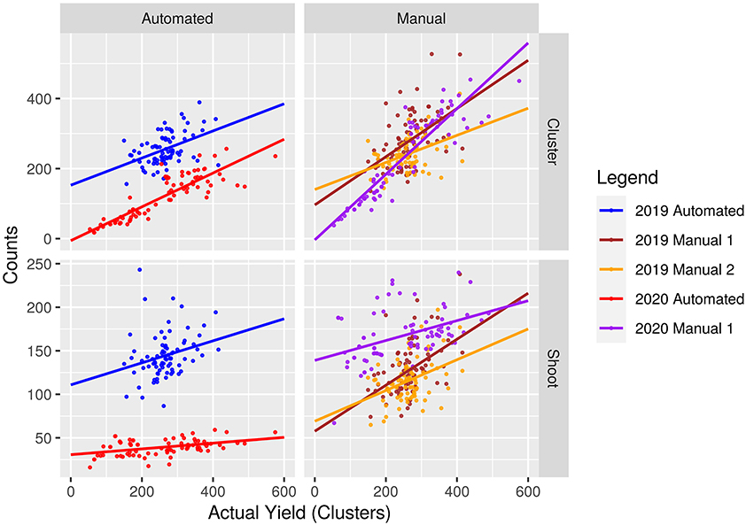
Figure 3. Manual and uncalibrated automated counts of clusters and shoots plotted against the actual number of clusters in each panel with lines of best fit.

TABLE 1

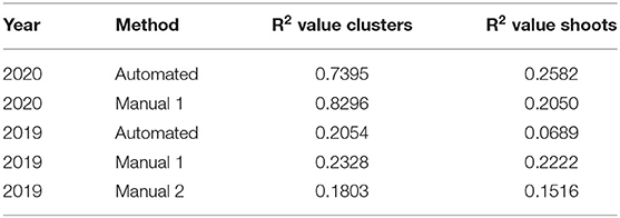
Table 1. R² values corresponding to the line of best fit for data presented in Figure 3.

TABLE 2

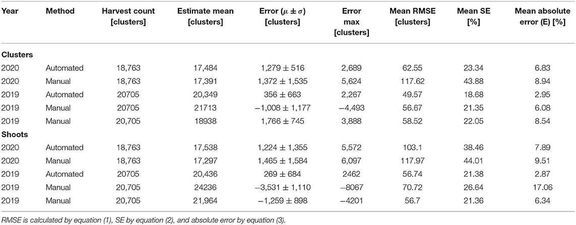
Table 2. Performance of each method for cluster count estimation method.

TABLE 3

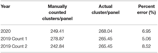
Table 3. Average number of clusters per panel, derived from counting all panels manually.

The average error of manual counts that leverage the null model vary depending on the specific counter. Analysis shows that in both 2019 and 2020, the proposed method, on average, shows less yield estimate error when counting grape clusters directly, as opposed to counting shoots. Furthermore, on average across both growing seasons, the calibrated automated counts of clusters predicted the yield with a mean error of 4.89 and 5.38% using clusters and shoots, respectively. In contrast, manual methods on averaged predicted yield with a mean error of 7.35 and 10.97% using clusters and shoots, respectively. The distribution of error for each model is presented in Figure 4.

FIGURE 4

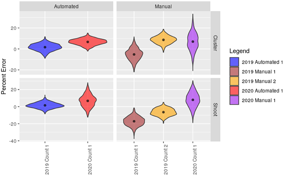
Figure 4. Distributions of percent error in cluster count prediction for automated and manual methods. The black dot represents the mean percent error.

Discussion

The manual count accuracy greatly depended on the counter. In our first experiment, we found that for a panel containing 320 clusters, the manual counts spanned from 237 to 309. Furthermore, the linear correlation between the manual counts and actual number of clusters in each panel for the entire dataset had R² values spanning from 0.18 to 0.83. Likewise, the relative square error of these counters spanned from 19.36 to 26.31%. Despite the relatively high error in manually counting panels, this method is still the most widely used in industry. Current recommendations for overcoming this problem are simply to sample a larger portion of the vineyard (Pool, 2001).

The automated method outperforms the manual method on both shoots and clusters. The reason why the automated method is able to perform with lower mean and max error is that it has a lower relative square error than the manual methods (Table 2). In essence, it can better account for the high variance in the number of clusters per panel than an average of a subset can.

The data suggests that counting clusters rather than shoots results in better performance for both automated and manual methods. While there is a positive correlation between the number of shoots and the number of clusters in a panel, the accuracy of the manual shoot counts were not able to be verified in the same way that the cluster counts were; it is unknown whether the poor performance of counting shoots was due to error on the part of the counter, or high variance in the number of clusters per shoot. For the automated counts, the difference in shoot counting error from 2019 to 2020 may be explained by the video capturing techniques. In 2019 the videos were captured with the camera mounted to an ATV, and the camera was further from the vines, capturing the entirety of all of the shoots. In 2020, the videos were collected by a different individual that held the camera and lights as they walked down the row, and on average the camera was held closer to the vine, cutting off more of the tops of the shoots from the frame. The performance of the automated estimates counting clusters, however, is robust against the variations in video capturing techniques.

When comparing our most reliable manual counter in the 2020 dataset against the automated method, the automated method only slightly outperforms the manual method. However, the error of the automated counts has a much smaller standard deviation, meaning the amount of error in the total cluster count estimate is less sensitive to which panels from the dataset are selected to be used for calibration, and results in a smaller max error than the manual counting method. For instance, in 2020, out of the 70 panels, the automated method was calibrated on 20 panels resulting in an error of −1,279 ± 516 clusters. In contrast, the manual counting method resulted in an error or −1,212 ± 1551 clusters.

While increasing the amount of calibration data would likely improve the performance of the automated method, further improvements may also be made to the software to increase the overall system performance. For instance, there are a variety of other object detection models that could be tested to improve performance. While Faster R-CNN, Single Shot Detector, ResNet50, and MobileNetV1 are widely used object detection model components, other popular object detectors such as ZFNet (Zeiler and Fergus, 2014), YOLO (Redmon et al., 2016), or RetinaNet (Lin et al., 2017), to name a few, may increase the performance of the system. While no formal performance metrics for the KCF tracker were collected, its performance was visually inspected and compared against MIL tracker (Babenko et al., 2009), MOSSE tracker (Bolme et al., 2010), and CSR tracker (Lukezic et al., 2017), with the KCF tracker showing the best performance. Alternative methods that fuse object detection with tracking in a single deep learning model, such as GOTURN (Held et al., 2016) or ROLO (Ning et al., 2017) may lead to increased performance of the system.

The automated counting method processed videos at 5 frames per second, or about 1–1.5 min per panel. The entire software framework is bundled into a stand-alone, easy to use, executable program that is capable of batch processing videos. Given current rates of cloud computing, acres of videos could be processed in a few hours for tens of dollars on services like Google Cloud or AWS. Final automated counts still need to be correlated to final yield using an aforementioned cluster weight estimation method such as historical values, Lag-Phase, or the Growing Degree Day Method. Transition to practice and wide scale use of this system is advanced by the object detection algorithm's ability to perform on cultivars it was not trained on. However, further generalizability could be achieved by open-sourcing image training data from different regions, cultivars, lighting conditions, and camera image sensors. We are currently investigating intellectual property licensing to companies in the agritech industry in an effort to disseminate this technology to grape growers. Our hope to make this technology available and easy to use for both small and large-scale grape growers.

Based on our experimental results using data from 2020, we found that the counters must count at least 50 panels to achieve the same accuracy as the automated method calibrated on 20 panels (Figure 5). The counters (in the experimental vineyard) spent an average 15 min per panel, amounting to almost 13 h for 50 panels, whereas counting 20 panels and imaging all 70 panels would take 5.3 h. As the vineyard size increases, the amount of time saved increases. New York state vineyards have anywhere from 160 to 200 panels per acre (Davis et al., 2020), therefore using our automated system for a 40 acre vineyard with 8,000 panels would lead to a decrease in labor time by two orders of magnitude (~100).

FIGURE 5

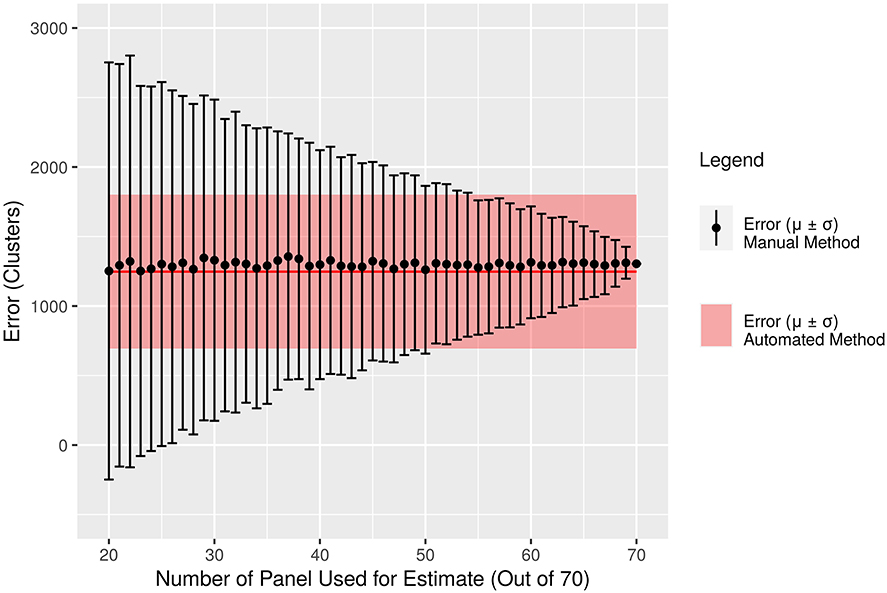
Figure 5. The mean error and standard deviation of the manual method are plotted in black for data collected in 2020. The standard deviation of the error decreases as the number of panels used is increased. The red line represents the mean error of the automated method on the same dataset but only using 20 panels. The red shaded region represents the standard deviation of the automated method using 20 panels.

In contrast to the work presented here, previous research in ground vehicle-based computer vision methods for yield estimation in grapes has been primarily focused on estimating the total weight of the yield, instead of just the cluster number. Aquino et al. (2018) achieved 12.83% relative square error across 30 panels (three vines/panel) and overall relative error close to 0 by detecting and counting individual berries. However, the data collection occurred later in the season, near EL phenological stages 29–31, after fruit set. Furthermore, it required the fruit to be completely exposed by stripping all the leaves from the fruit zone, the use of $1,000 mirrorless DSLR camera, an inductive sensor installed on the ATV to trigger the camera, and a custom-built electronic control system to merge image and GPS data; requirements that make implementation impossible or impractical for many grape growers.

Efforts to enable improved yield estimation using readily available and cheap hardware, such as smartphones have been made by Grossetete et al. (2012). However, this work was focused on non-destructively imaging grape clusters after floration and using CV to count the number of berries per cluster, a value that can indicate the average cluster weight. Alternatively, Cunha et al. (2010) derived methods that use SPOT satellite imaging to predict useful yield estimates up to 17 months in advance. However, the vegetation data from SPOT has a spatial resolution of ~km, making this method impractical for many small vineyards.

The need for low-cost, easy to use, and inexpensive methods for increasing the accuracy of early-stage yield predictions in vineyards is driven by a competitive high-value crop market and the larger economic impacts of the grape and wine industry worldwide. The proposed computer vision-based method has lower setup and operational costs than other CV methods, less labor time than traditional methods, and operates during the pre-bloom stage, while offering higher reliability in cluster count estimates than traditional methods. These factors, along with the system's simplicity and ease of use, lower the barrier to entry for computer vision agritech use in smaller vineyards.

Data Availability Statement

The raw data supporting the conclusions of this article will be made available by the authors, without undue reservation.

Author Contributions

KP and JV developed the original idea for this work and acquired the funding. JJ, JV, and KP contributed to the experimental design and contributed to the data interpretation. JJ performed the field work and data analyses, wrote the first version of the manuscript, and revised and edited the manuscript. All authors approved the submitted version.

Funding

This work was supported by NSF grant #1837367 CPS: TTP Option: Medium: Touch Sensitive Technologies for Improved Vineyard Management and NIFA grant #1014705 Improving Vineyard Management Using Touch Sensitive Soft Robots.

Conflict of Interest

The authors declare that the research was conducted in the absence of any commercial or financial relationships that could be construed as a potential conflict of interest.

Acknowledgments

We would like to thank Ryan O'Hern for implementing an early version of the physical and software implementation. We further thank Anne Kearney, Justin Jackson, and Alex Siskovic for their help with field counting, video collection, and image labeling.

Footnotes

1. ^tensorflow.org.

2. ^github.com/tzutalin/labelImg.

3. ^opencv.org.

References

Aquino, A., Millan, B., Diago, M., and Tardaguila, J. (2018). Automated early yield prediction in vineyards from on-the-go image acquisition. Comp. Electr. Agricult. 144, 26–36. doi: 10.1016/j.compag.2017.11.026

CrossRef Full Text | Google Scholar

Atzberger, C. (2013). Advances in remote sensing of agriculture: context description, existing operational monitoring systems and major information needs. Remote Sens. 5, 949–981. doi: 10.3390/rs5020949

CrossRef Full Text | Google Scholar

Babenko, B., Yang, M., and Belongie, S. (2009). “Visual tracking with online multiple instance learning,” in 2009 IEEE Conference on computer vision and Pattern Recognition (Miami, FL: IEEE), 983–990. doi: 10.1109/CVPR.2009.5206737

PubMed Abstract | CrossRef Full Text | Google Scholar

Bolme, D. S., Beveridge, J. R., Draper, B. A., and Lui, Y. M. (2010). “Visual object tracking using adaptive correlation filters,” in 2010 IEEE Computer Society Conference on Computer Vision and Pattern Recognition (San Francisco, CA: IEEE), 2544–2550. doi: 10.1109/CVPR.2010.5539960

PubMed Abstract | CrossRef Full Text | Google Scholar

Cunha, M., Marcal, A. R. S., and Silva, L. (2010). Very early prediction of wine yield based on satellite data from VEGETATION. Int. J. Remote Sen.s 31, 3125–3142. doi: 10.1080/01431160903154382

CrossRef Full Text | Google Scholar

Dami, I., and Sabbatini, P. (2011). Crop estimation of grapes. Columbus, OH: The Ohio State University Fact Sheet.

Google Scholar

Davis, T. J., Gómez, M. I., Russell, M., and Hans, W. P. (2020). Cost of Establishment and production of V. Vinifera grapes in the Finger Lakes region of New York-2019 (Ithaca, NY).

Google Scholar

Eichhorn, V. K. W., and Lorenz, D. H. (1977). Phenological Development Stages of the Grapewine, 28–29.

Google Scholar

Grossetete, M., Berthoumieu, Y., Costa, J. P. D., Germain, C., Lavialle, O., and Grenier, G. (2012). “Early estimation of vineyard yield: site specific counting of berries by using a smartphone,” in International Conference of Agricultural Engineering—CIGR-AgEng, (Valencia).

Google Scholar

He, K., Zhang, X., Ren, S., and Sun, J. (2016). “Deep residual learning for image recognition,” in Proceedings of the IEEE Conference on Computer Vision and Pattern Recognition (Las Vegas, NV), 770–778. doi: 10.1109/CVPR.2016.90

PubMed Abstract | CrossRef Full Text | Google Scholar

Held, D., Thrun, S., and Savarese, S. (2016). “Learning to track at 100 fps with deep regression networks,” in European Conference on Computer Vision Cham: Springer), 749–765. doi: 10.1007/978-3-319-46448-0_45

CrossRef Full Text | Google Scholar

Henriques, J. F., Caseiro, R., Martins, P., and Batista, J. (2014). High-speed tracking with kernelized correlation filters. IEEE Trans. Pattern Anal. Mach. Intell. 37, 583–596. doi: 10.1109/TPAMI.2014.2345390

PubMed Abstract | CrossRef Full Text | Google Scholar

Kuhn, H. W. (1955). The Hungarian method for the assignment problem. Naval. Res. Log. Q. 2, 83–97. doi: 10.1002/nav.3800020109

CrossRef Full Text | Google Scholar

Lin, T., Goyal, P., Girshick, R., He, K., and Dollár, P. (2017). “Focal loss for dense object detection,” in Proceedings of the IEEE International Conference on Computer Vision (Venice), 2980–2988. doi: 10.1109/ICCV.2017.324

PubMed Abstract | CrossRef Full Text | Google Scholar

Lukezic, A., Vojir, T., Zajc, L. C., Matas, J., and Kristan, M. H. (2017). “Discriminative correlation filter with channel and spatial reliability,” in Proceedings of the IEEE Conference on Computer Vision and Pattern Recognition (Honolulu, HI), 6309–6318. doi: 10.1109/CVPR.2017.515

CrossRef Full Text | Google Scholar

Ma, J., Da-Wen, S., Jia-Huan, Q., Dan, L., Hongbin, P., Wen-Hong, G., et al. (2016). Applications of computer vision for assessing quality of agri-food products: a review of recent research advances. Crit. Rev. Food Sci. Nutr. 56, 113–127. doi: 10.1080/10408398.2013.873885

PubMed Abstract | CrossRef Full Text | Google Scholar

Ning, G., Zhang, Z., Huang, C., Ren, X., Wang, H., Cai, C., et al. (2017). “Spatially supervised recurrent convolutional neural networks for visual object tracking,” in 2017 IEEE International Symposium on Circuits and Systems (ISCAS) (IEEE), 1–4. doi: 10.1109/ISCAS.2017.8050867

CrossRef Full Text | Google Scholar

Pool, R. (2001). Estimating and Adjusting Crop Yield in the Finger Lakes Vineyards. Ithaca, NY.

Redmon, J., Divvala, S., Girshick, R., and Farhadi, A. (2016). “You only look once: unified, real-time object detection,” in Proceedings of the IEEE Conference on Computer Vision and Pattern Recognition (Las Vegas, NV), 779–788. doi: 10.1109/CVPR.2016.91

CrossRef Full Text | Google Scholar

Ren, S., He, K., Girshick, R., and Sun, J. (2016). Faster r-cnn: Towards real-time object detection with region proposal networks. IEEE Trans. Pattern Anal. Mach. Intell. 39, 1137–1149. doi: 10.1109/TPAMI.2016.2577031

PubMed Abstract | CrossRef Full Text | Google Scholar

Rist, F., Herzog, K., Mack, J., Richter, R., Steinhage, V., and Töpfer, R. (2018). High-precision phenotyping of grape bunch architecture using fast 3D sensor and automation. Sensors 18:763. doi: 10.3390/s18030763

PubMed Abstract | CrossRef Full Text | Google Scholar

Rose, J. C., Kicherer, A., Wieland, M., Klingbeil, L., Töpfer, R., and Kuhlmann, H. (2016). Towards automated large-scale 3D phenotyping of vineyards under field conditions. Sensors 16:2136. doi: 10.3390/s16122136

PubMed Abstract | CrossRef Full Text | Google Scholar

Seng, K. P., Ang, L., Schmidtke, L. M., and Rogiers, S. Y. (2018). Computer vision and machine learning for viticulture technology. IEEE Access 6, 67494–67510. doi: 10.1109/ACCESS.2018.2875862

CrossRef Full Text | Google Scholar

Wolf, T. K. (2008). Wine Grape Production Guide for Eastern North America. Ithaca, NY.

Zeiler, M. D., and Fergus, R. (2014). “Visualizing and understanding convolutional networks,” in European Conference on Computer Vision (Cham: Springer), 818–833. doi: 10.1007/978-3-319-10590-1_53

CrossRef Full Text | Google Scholar