A Finite Element Analysis of the Stability of Composite Beams With Arbitrary Curvature

Introduction

Laminated composite (fiber-reinforced) structures are increasingly used in a wide range of engineering applications (naval, aeronautical, automation, mechanical, civil, medical engineering, etc.), due to the outstanding proprieties that such structures may exhibit when a proper design of the material and the lamination scheme are employed: light weight, high stiffness-to-weight and tensile strength-to-weight ratios, high damping, excellent corrosion, thermal and high impact resistance (Fraternali et al., 2011, 2012; Bencardino et al., 2012). Nowadays, laminated composite structures play a crucial role in the production of various innovative structures or products, which include: light-weight roof structures, arch bridges, impact energy mitigation and vibration isolation devices, just to name a few examples. In order to capture the puzzling mechanical response of such structures, various theoretical and numerical approaches have been proposed in the literature, including zig-zag displacement-based theories and stress-based methods, with special attention on the modeling of anisotropy, warping, fracture and damage (Feo and Fraternali, 2000; Roberts and Al-Ubaidi, 2001; Fraternali et al., 2002, 2010, 2011, 2012; Fraternali, 2007; Schmidt et al., 2009; Feo and Mancusi, 2010; Bencardino et al., 2012; Markkula et al., 2013; Viera et al., 2013; Özütok and Madenci, 2017). Shear deformation and warping effects may be rather important in composite beams. At this regard (Özütok and Madenci, 2017) by Özütok and Madenci analyses the effects of a non-linear distribution of the shear stress through the beam thickness within a higher-order shear deformation theory; Roberts and Al-Ubaidi develop in Roberts and Al-Ubaidi (2001) an approximate theory for assessing the influence of shear deformation on restrained torsional warping of pultruded bars; while Viera et al. develop a thin-walled beam model able to simulate warping and higher order effects in Viera et al. (2013). For what concerns stability phenomena, which are of peculiar interest in the case of composite beams due to the characteristic slenderness of such structures, it is worth mentioning the non-linear elastic approaches proposed in Ascione et al. (2011, 2013); Fraternali et al. (2013); Mascolo and Pasquino (2016); Özütok and Madenci (2017), and Mascolo et al. (in press). The recent study illustrated in Fraternali et al. (2013) presents a geometrically nonlinear theory of laminated curved beams, which assumes that cross-section rotations and shear strains are moderately large, while axial strains are infinitesimal. Due to its minor complexity with respect to the finite elasticity theory, the model presented in Fraternali et al. (2013) is particularly convenient for computing the first stability point of a composite laminated beam and studying its behavior near such a point.

In the present paper, we develop a comprehensive finite-element approximation of the mechanical model given in Fraternali et al. (2013), which is founded upon the use of Lagrangian isoparametric elements (section Finite Element Model). The adopted model proves to be a robust and versatile tool that allows to model the geometrically non-linear response and the buckling behavior of laminated composite beams with arbitrary curvature. It takes into account both shear deformations and warping effects, which are essential to accurately predict in-plane and out-plane buckling loads. The proposed stability analysis employs the path-following procedure proposed by Bathoz and Dhatt (1979) and the algorithm for computing stability points proposed by Simo and Wriggers (1990) (section Finite Element Analysis of the Stability of Composite Curved Beams). The accuracy of the proposed finite-element model is assessed by presenting different numerical results relative to the stability of isotropic and composite beams and establishing comparisons with the corresponding results of classical beam theories and other theories available in the relevant literature (section Numerical Results). We end with concluding remarks and directions for future work in section Concluding Remarks.

Finite Element Model

Let us denote by C^h a finite-element discretization of axis curve of a laminated beam, and let us assume that the elements C₁, …, C_n belong to the Lagrange family (Reddy, 1992) (see Figure 1)

$\begin{array}{cc}{C}^h={{\displaystyle \cup }}_{e=1}^{n_e}{C}_e.& (1)\end{array}$

FIGURE 1

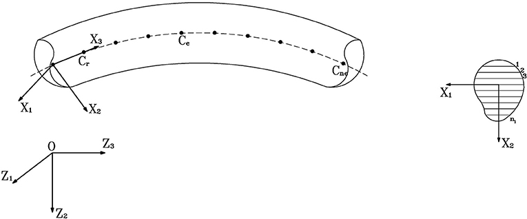
Figure 1. Finite element discretization of the axis of a laminate curved beam (n_l: numbers of layers).

On adopting an isoparametric finite-element approximation (Reddy, 1992) we use the same shape functions to approximate both the geometry and the (generalized) displacement field over the generic element C_e

$\begin{array}{cc}{Z}_{2_e}^h={\displaystyle {\displaystyle \sum }_{I=1}^n}{N}_I{Z}_{2_I,}{Z}_{3_e}^h={\displaystyle {\displaystyle \sum }_{I=1}^n}{N}_I{Z}_{3_I,}{\widehat{u}}_e^h={\displaystyle {\displaystyle \sum }_{I=1}^n}{N}_I{\widehat{u}}_I.& (2)\end{array}$

In Equation (2) N_I is the shape function corresponding to the node I and consists of a complete polynomial of order n − 1; Z_2I and Z_3I are the coordinates of I with respect to the global frame {0, Z₁, Z₂, Z₃} (Figure 1); ${\widehat{u}}_I$ is the generalized displacement vector relative to the same node.

In particular, for a four-node Lagrangian element, we represent in Figure 2 the transformation (2)_1,2 which maps the master element onto a curved (cubic) element.

FIGURE 2

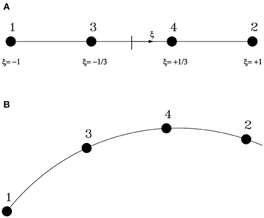
Figure 2. Standard (A) and distorted (B) four-node Lagrangian element.

The Jacobian of the transformation from the local coordinate ξ (Figure 2) to the global coordinate X₃ (Figure 1) is given by Nomizu and Kobayashi (1963)

$\begin{array}{cc}\begin{array}{l}J=\frac{d{X}_3}{d\xi }=\sqrt{{\left(\frac{d{Z}_{2_e}^h}{d\xi }\right)}^2+{\left(\frac{d{Z}_{3_e}^h}{d\xi }\right)}^2}\hfill \\ =\sqrt{{\left({\displaystyle {\displaystyle \sum }_{I=1}^n}{N}_{I,\xi }{Z}_{2_I}\right)}^2+{\left({\displaystyle {\displaystyle \sum }_{I=1}^n}{N}_{I,\xi }{Z}_{3_I}\right)}^2}\hfill \end{array}& (3)\end{array}$

N_{I, ξ} being the derivative of N_I with respect to ξ. Denoting by (·)′ the derivative with respect to X₃, we have:

$\begin{array}{cc}{N}_I^{\prime }=\frac{d{N}_I}{d{X}_3}=J^{-1}{N}_{1,\xi }.& (4)\end{array}$

By making use of Equation (2)_1,2, we obtain the following approximation of the curvature radius R (Nomizu and Kobayashi, 1963)

$\begin{array}{cc}{R}_e^h=\frac{{\left[{\left(Z_{2_e}^h\right)}_{,\text{ξ}}^2+{\left(Z_{3_e}^h\right)}_{,\text{ξ}}^2\right]}^{3/2}}{\left[{\left(Z_{2_e}^h\right)}_{,\text{ξ}}{\left(Z_{3_e}^h\right)}_{,\text{ξξ}}-{\left(Z_{2_e}^h\right)}_{,\text{ξξ}}{\left(Z_{3_e}^h\right)}_{,\text{ξ}}\right]}=\frac{{\left[{\left({\displaystyle {\sum }_{I=1}^n{N}_{I,\text{ξ}}{Z}_{2_I}}\right)}^2+{\left({\displaystyle {\sum }_{I=1}^n{N}_{I,\text{ξ}}{Z}_{3_I}}\right)}^2\right]}^{3/2}}{\left[\left({\displaystyle {\sum }_{I=1}^n{N}_{I,\text{ξ}}{Z}_{2_I}}\right)\left({\displaystyle {\sum }_{J=1}^n{N}_{J,\text{ξξ}}}{Z}_{3_J}\right)-\left({\displaystyle {\sum }_{I=1}^n{N}_{I,\text{ξξ}}{Z}_{2_I}}\right)\left({\displaystyle {\sum }_{J=1}^n{N}_{J,\text{ξ}}}{Z}_{3_J}\right)\right]}.& (5)\end{array}$

Coming back to Equation (2)₃, we now observe that it can be written in the following compact form

$\begin{array}{cc}{\widehat{u}}_e^h= N{U}_e& (6)\end{array}$

where U_e is the M-dimensional vector collecting nodal, generalized, displacements of

$\begin{array}{cc}{C}_e(U_e={[{\widehat{u}}_1^T,{\widehat{u}}_2^T,\dots ,{\widehat{u}}_n^T]}^T),& (7)\end{array}$

while N is the following matrix

$\begin{array}{cc}{N}_{[m\times M]}=[N_1,N_2,\dots ,N_n],& (8)\end{array}$

whose blocks are diagonal submatrices

$\begin{array}{cc}{N}_{I_{[m\times m]}}=diag(N_I{N}_I\dots N_I).& (9)\end{array}$

Equation (6) leads us to obtain the following approximation of the generalized strains

$\begin{array}{cc}{\widehat{E}}_e^h(U_e)={\widehat{E}}_e^{(1)h}(U_e)+\frac{1}{2}{\widehat{E}}_e^{(2)h}(U_e,U_e)& (10)\end{array}$

where

$\begin{array}{cc}\begin{array}{l}{\widehat{E}}_e^{(1)h}(U_e)=B_o{U}_e\hfill \\ {\widehat{E}}_e^{(2)h}(U_e,\delta U_e)=B_L(U_e)\delta U_e\hfill \end{array}& (11)\end{array}$

$\begin{array}{c}{B}_0\text{ and }{B}_L\left(U_e\right)\text{ being the following }\sigma \times M\text{ matrices}\\ \begin{array}{l}{B}_0=[B_{0_1},B_{0_2},\dots ,B_{0_n}],\hfill \\ B_L(U_e)=A(U_e)G.\hfill \end{array}& (12)\end{array}$

The σ × m submatrices B_0I in Equation (12)₁ are given by

$\begin{array}{ll}{B}_{o_I}=\left[\begin{array}{ccc}{B}_{o_I}^{E\nu }& {\text{B}}_{o_I}^{E\phi }& 0\\ 0& B_{o_I}^{\Theta \varphi }& 0\\ 0& 0& 0\\ 0& 0& B_{o_I}^{ww}\\ 0& 0& B_{o_I}^{w^{\prime }{w}^{\prime }}\end{array}\right]\text{ ,}& (13)\end{array}$

where

$\begin{array}{ll}{B}_{o_I}^{E\nu }=B_{o_I}^{\Theta \varphi }=\left[\begin{array}{ccc}{N^{\prime }}_1& 0& 0\\ 0& {N^{\prime }}_1& N_1/R\\ 0& -N_1/R& {N^{\prime }}_1\end{array}\right],& B_{o_I}^{E\phi }=\left[\begin{array}{ccc}0& {-N}_1{ }^{\prime }& 0\\ N_1& 0& 0\\ 0& 0& 0\end{array}\right],\\ B_{o_I}^{ww}{ }_{[m_w\times m_w]}=diag\left(N_I{N}_I\dots N_I\right),\\ B_{o_I}^{w^{\prime }{w}^{\prime }}{ }_{[m_w\times m_w]}=diag({N^{\prime }}_1{N^{\prime }}_1\dots {N^{\prime }}_1).& (14)\end{array}$

The matrices A and G, which appear in Equation (12)₂, are instead given by

$\begin{array}{ll}A{\left(U_e\right)}_{\left[\sigma \times 9\right]}=\left[\begin{array}{c}A\left(U_e\right)\\ 0\end{array}\right],G_{\left[9\times M\right]}=\left[G_{1,}{G}_{2,}\dots ,G_n\right],& (15)\end{array}$

where

$\begin{array}{ll}{G}_I{ }_{\left[9\times m\right]}=\left[{\overline{G}}_{I,}0\right],{\overline{G}}_I{ }_{\left[9\times 6\right]}=\left[\begin{array}{cccccc}{N}_1{ }^{\prime }& 0& 0& 0& 0& 0\\ 0& N_1{ }^{\prime }& 0& 0& 0& 0\\ 0& 0& N_1& 0& 0& 0\\ 0& 0& 0& N_1& 0& 0\\ 0& 0& 0& 0& N_1& 0\\ 0& 0& 0& 0& 0& N_1\\ 0& 0& 0& N_1{ }^{\prime }& 0& 0\\ 0& 0& 0& 0& N_1{ }^{\prime }& 0\\ 0& 0& 0& 0& 0& N_1{ }^{\prime }\end{array}\right],& (16)\end{array}$

$\begin{array}{l}A{\left(U_e\right)}_{\left[9\times 9\right]}=\\ \left[\begin{array}{ccccccccc}0& {\varphi }_3& \frac{{\varphi }_3}{R}& \frac{{\varphi }_3}{2}& 0& \left(v_2{ }^{\prime }+\frac{v_3}{R}+\frac{{\varphi }_1}{2}\right)& 0& 0& 0\\ -{\varphi }_3& 0& 0& 0& \frac{{\varphi }_3}{2}& \left(-v_1{ }^{\prime }+\frac{{\varphi }_2}{2}\right)& 0& 0& 0\\ v_1{ }^{\prime }& \left(v_2{ }^{\prime }+\frac{v_3}{R^2}\right)& \left(\frac{v_2{ }^{\prime }}{R}+\frac{v_3}{R^2}\right)& 0& 0& 0& 0& 0& 0\\ \left(-{\varphi }_3{ }^{\prime }+\frac{{\varphi }_2}{R}\right)& 0& 0& 0& \left(\frac{v_1{ }^{\prime }}{R}+\frac{{\varphi }_2}{R}+\frac{{\varphi }_3{ }^{\prime }}{2}\right)& \left(\frac{{\varphi }_2{ }^{\prime }}{2}+\frac{{\varphi }_3}{R}\right)& 0& \frac{{\varphi }_3}{2}& \left(-v_1{ }^{\prime }+\frac{{\varphi }_2}{2}\right)\\ 0& \left(-{\varphi }_3{ }^{\prime }+\frac{{\varphi }_2}{R}\right)& \left(-\frac{{\varphi }_3{ }^{\prime }}{R}+\frac{{\varphi }_2}{R^2}\right)& \left(-\frac{{\varphi }_3{ }^{\prime }}{2}+\frac{{\varphi }_2}{2R}\right)& \left(\frac{v_2{ }^{\prime }}{2}+\frac{v_3}{R^2}+\frac{{\varphi }_1}{2R}\right)& -\frac{{\varphi }_1{ }^{\prime }}{2}& -\frac{{\varphi }_3}{2}& 0& \left(-v_2{ }^{\prime }-\frac{v_3}{R}-\frac{{\varphi }_1}{2}\right)\\ 0& 0& 0& \left(-\frac{{\varphi }_2{ }^{\prime }}{2}+\frac{{\varphi }_3}{2R}\right)& -\frac{{\varphi }_1{ }^{\prime }}{2}& -\frac{{\varphi }_1}{2R}& \frac{{\varphi }_2}{2}& -\frac{{\varphi }_1}{2}& 0\\ 0& 0& 0& 0& \left(-\frac{{\varphi }_3{ }^{\prime }}{R}+\frac{{\varphi }_2}{R^2}\right)& \left(-\frac{{\varphi }_2{ }^{\prime }}{R}+\frac{{\varphi }_3}{R^2}\right)& 0& \left(-{\varphi }_2{ }^{\prime }+\frac{{\varphi }_3}{R}\right)& \left(-{\varphi }_3{ }^{\prime }+\frac{{\varphi }_2}{R}\right)\\ 0& 0& 0& 0& \left(-\frac{{\varphi }_3{ }^{\prime }}{R}+\frac{{\varphi }_2}{R^2}\right)& 0& {\varphi }_1{ }^{\prime }& 0& \left(-{\varphi }_3{ }^{\prime }+\frac{{\varphi }_2}{R}\right)\\ 0& 0& 0& 0& 0& -\frac{{\varphi }_1{ }^{\prime }}{R}& \left(-{\varphi }_2{ }^{\prime }+\frac{{\varphi }_3}{R}\right)& {\varphi }_1{ }^{\prime }& 0\end{array}\right]& (17)\end{array}$

Finite Element Analysis of the Stability of Composite Curved Beams

Path-Following Procedure

Let us consider the variational formulation of the equilibrium equations. The use of Equations (6, 10, 11) allows us to set such equations into the following discrete form

$\begin{array}{l}\begin{array}{ccc}\delta {\Pi }^h& =& \delta U^{T}R(U,\lambda )\end{array}\\ ={\displaystyle {\sum }_{e=1}^{n_e}\left\{\delta U_e^T{\displaystyle {\int }_{-1}^1\left[B_0^T+B_L^T\left(U_e\right)\right]\widehat{D}\left[B_0+\frac{1}{2}{B}_L\left(U_e\right)\right]}{U}_{e}Jd\xi \right\}}\\ -\lambda {\displaystyle \sum _{e=1}^{n_e}\left\{\delta U_e^T{\displaystyle {\int }_{-1}^1{N}^T\left[{\widehat{q}}_e^{\left(1\right)}+{\widehat{q}}_e^{\left(2\right)}\left(U_e\right)\right]Jd\xi }\right\}}\\ -\lambda {\displaystyle \sum _{I=1}^{n_n}\left\{\delta {\widehat{u}}_I^T\left[{\widehat{Q}}_I^{\left(1\right)}+{\widehat{Q}}_I^{\left(2\right)}\left({\widehat{u}}_I\right)\right]\right\}=0}& (18)\end{array}$

where Π^h is the discretized functional of the total potential energy Π; δΠ^h is the first variation of Π^h with increment δU; R(U, λ) (residuai vector) is the Gateaux derivative of Π^h with respect to $U(R=D_U{\Pi }^h)$.

On accounting for a possibility of non-linear elastic response of the material, we assume that the elasticity matrix $\widehat{D}$, whose elements are the resultants and the resultant moments of the local elastic moduli (Fraternali et al., 2013), depends on the deformation of the beam ($\widehat{\text{D}}$ = $\widehat{\text{D}}(U)$).

Equation (18) can also be written in the following compact form

$\begin{array}{ll}\delta U^{T}R\left(U,\lambda \right)=\delta U^T\left\{K\left(U\right)U-\lambda \left[Q^{\left(1\right)}+Q^{\left(2\right)}\left(U\right)\right]\right\}=0,& (19)\end{array}$

where K(U) is the N × N global (secant) stiffness matrix, which derives from the assembly of the element stiffness matrices K_e (e = 1, 2, …, n_e). Such matrices are defined by the equations

$\begin{array}{ll}{K}_e\left(U_e\right)\left(U_e\right)={\displaystyle {\int }_{-1}^1\left[B_0^T+B_L^T\left(U_e\right)\right]}\widehat{S}\left(U_e\right)Jd\xi ,& (20)\end{array}$

where $\widehat{S}$ is the generalized stress vector

$\begin{array}{ll}\widehat{S}\left(U_e\right)=\widehat{D}\left[B_0+\frac{1}{2}{B}_L\left(U_e\right)\right]U_e,& (21)\end{array}$

while Q⁽¹⁾ and Q⁽²⁾(U) are the global force vectors, which derive from the assembly of the element vectors

$\begin{array}{ll}{Q}_e^{(1)}={\displaystyle {\int }_{-1}^1{N}^T{\widehat{q}}_e^{(1)}}Jd\xi ,Q_e^{(2)}\left(U_e\right)={\displaystyle {\int }_{-1}^1{N}^T{\widehat{q}}_e^{(2)}\left(U_e\right)}Jd\xi ,& (22)\end{array}$

and the nodal force vectors ${\widehat{Q}}_I^{(1)}$ and ${\widehat{Q}}_I^{(2)}({\widehat{u}}_I)(I=1,2,\dots ,n_n)$.

Due to the arbitrariness of δU, Equation (19) is equivalent to the following nonlinear system of N equations

$\begin{array}{ll}R\left(U,\lambda \right)=K\left(U\right)U-\lambda \left[Q^{\left(1\right)}+Q^{(2)}\left(U\right)\right]=0,& (23)\end{array}$

which can be solved by employing one of the algorithms known in literature as path-following methods (for an overview of such methods (see e.g., Riks, 1972). The basic idea of path-following methods is to append a constraint Equation f(U, λ) = 0 to (23). Here, following Bathoz and Dhatt (1979), we adopt a displacement control and assume

$\begin{array}{ll}f\left(U\right)=e_p^{T}U-\text{u}=0,& (24)\end{array}$

where e_p is the vector of ℜ^N which has only the pth component different from zero and equal to 1, while μ is a prescribed value of the pth component of U. Therefore, we are led to solve the extended system

$\begin{array}{cc}{\mathit{R}}^{\ast }\left(\mathit{U},\lambda \right)=\left\{\begin{array}{c}\mathit{R}\left(\mathit{U},\lambda \right)\\ {\mathit{e}}_p^T\mathit{U}-\text{ μ}\end{array}\right\}=0,& (25)\end{array}$

The linearization of Equation (25) by the Newton-Raphson method gives the system of incremental equilibrium equations

$\begin{array}{cc}{\mathit{R}}^{\ast }\left(\mathit{U}+\Delta \mathit{U},\lambda +\Delta \lambda \right)={\mathit{R}}^{\ast }\left(\mathit{U},\lambda \right)+\left[\begin{array}{cc}{D}_U\mathit{R}& D_{\lambda }\mathit{R}\\ {\mathit{e}}_p^T& 0\end{array}\right]\left\{\begin{array}{c}\Delta \mathit{U}\\ \Delta \lambda \end{array}\right\}=0,& (26)\end{array}$

The matrix D_UR, which is usually referred to as tangent stiffness matrix and denoted by K_T, is given in the Appendix. Concerning the vector D_λR, from Equation (23) we deduce

$\begin{array}{cc}{D}_{\lambda }\mathit{R}=-\left[{\mathit{Q}}^{\left(1\right)}+{\mathit{Q}}^{\left(2\right)}\left(\mathit{U}\right)\right].& (27)\end{array}$

The non-symmetric system (26), that we rewrite in the form

$\begin{array}{cc}\left[\begin{array}{cc}{\mathit{K}}_T& -\left({\mathit{Q}}^{\left(1\right)}+{\mathit{Q}}^{(2)}\right)\\ {\mathit{e}}_p^T& 0\end{array}\right]\left\{\begin{array}{c}\Delta \mathit{U}\\ \Delta \lambda \end{array}\right\}=-\left\{\begin{array}{c}\mathit{R}\left(\mathit{U},\lambda \right)\\ {\mathit{e}}_p^T\mathit{U}-\mathbf{\mu }\end{array}\right\},& (28)\end{array}$

can be solved by a procedure known in literature as bordering algorithm (see e.g., Keller, 1977). Such algorithm and the overall procedure for the solution of the extended system (25) are described in Table 1.

TABLE 1

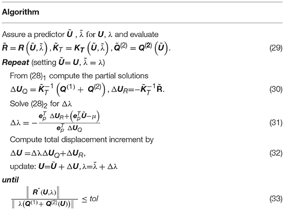
Table 1. Bordering algorithm.

In particular, if the first predictor U satisfies the constraint (24), Equation (31) reduces to

$\begin{array}{cc}\Delta \text{λ}=\frac{e_p^T\Delta U_R}{e_p^T\Delta U_Q}& (34)\end{array}$

We point out that, since we proceed by displacement control, we apply the above iterative procedure in incremental steps. Within the generic step, say the ith one, we increment by δ the displacement component U_p which exhibited the largest variation in the previous step. We hence set in the extended system (25)

$\begin{array}{cc}\mu ={\text{e}}_p^T{U}^{i-1}+\delta & (35)\end{array}$

and begin the new iteration loop by assuming the predictor $\tilde{U}=U^{i-1}+\delta e_p$, $\tilde{\lambda }={\lambda }^{i-1}$, which satisfies Equation (24).

Computation of Stability Points

In the current section we get a finite-element approximation of the problem of computing stability points based on the Trefftz criterion (Trefftz, 1930).

Within the previous settings, we obtain the following discrete equation

$\begin{array}{cc}{D}_U^2{\displaystyle {\prod }_e^h\left(U,\text{λ}\right)}{U}_1\delta U=\delta U^T{K}_T\left(U,\text{λ}\right)U_1=0& (36)\end{array}$

which must be satisfied by every variation δU.

A point U, λ such that Equation (36) holds for some U₁ is usually called stability point, while U₁ is called buckling mode (or eigenvector) associated with U, λ.

Due to the arbitrariness of δU, Equation (36) is equivalent to the system of N Equations

$\begin{array}{cc}{K}_T\left(U,\lambda \right)U_1=0& (37)\end{array}$

In the following we will denote U₁ by V. In order to exclude the trivial case V=0, it is necessary to append a constraint equation l(V)=0 to system (37). Possible choices of such an equation are

$\begin{array}{cc}\Vert V\Vert -1=0& (38)\end{array}$

$\begin{array}{cc}{e}_p^{T}V-V_0=0& (39)\end{array}$

V₀ being a fixed (non-zero) value of the pth component of V. In this work we make use of Equation (39) and, after having reduced K_T to an upper triangular matrix (by Gauss elimination technique), we identify the index p with the equation number where the lowest diagonal term of the reduced stiffness matrix appears. In this way we prevent the pth component of V becoming exceedingly large. Concerning V₀, we set

$\begin{array}{cc}{V}_0=\frac{e_p^T{V}_0}{\Vert V_0\Vert }& (40)\end{array}$

V₀ being the initial approximation to V.

Stability points can be classified in limit (or turning) and bifurcation points (Budiansky, 1974). Following Spence and Jepson (Spence and Jepson, 1985) we can distinguish between the two cases by using the following criteria

$\begin{array}{cc}\text{Bifurcation point}:V^T\left(Q^{\left(1\right)}+Q^{(2)}\left(U\right)\right)=0& (41)\end{array}$

$\begin{array}{cc}\text{Limit point}:V^T\left(Q^{\left(1\right)}+Q^{(2)}\left(U\right)\right)\ne 0& (42)\end{array}$

An efficient procedure for the computation of stability points has been proposed by Simo and Wriggers (1990). It consists of solving the extended system

$\begin{array}{cc}{R}^{\ast \ast }\left(U,V,\lambda ,\mu \right)=\left\{\begin{array}{c}R\left(U,\lambda \right)\\ K_T\left(U,\lambda \right)V\\ e_p^{T}V-V_0\\ e_p^{T}U-\mu \end{array}\right\}=0& (43)\end{array}$

which derives from the addition of Equations (37, 39) to the system of non-linear equilibrium Equations (25).

Since the tangent stiffness matrix becomes progressively ill-conditioned as the solution approaches the stability point, where K_T is singular, from a numerical point of view it is convenient to transform the extended system (43) into the following equivalent form Simo and Wriggers (1990)

$\begin{array}{cc}{R}_{\eta }^{\ast \ast }\left(U,V,\lambda ,\mu \right)=\left\{\begin{array}{c}R\left(U,\lambda \right)+\eta \left(e_p^{T}U-\mu \right)e_p\\ K_T\left(U,\lambda \right)V+\eta \left(e_p^{T}V-V_0\right)e_p\\ e_p^{T}V-V_0\\ e_p^{T}U-\mu \end{array}\right\}=0,& (44)\end{array}$

η being an arbitrary positive number. The linearization of Equation (44) by the Newton-Raphson method leads us to obtain the set of incremental equations

$\begin{array}{c}\left[\begin{array}{cccc}{K}_{T_{\eta }}& 0& -Q& -\eta e_p\\ D_U\left(K_{T}V\right)& K_{T_{\eta }}& D_{\lambda }\left(K_{T}V\right)& 0\\ 0^T& e_p^T& 0& 0\\ e_p^T& 0^T& 0& -1\end{array}\right]\left\{\begin{array}{c}\Delta U\\ \Delta V\\ \Delta \lambda \\ \Delta \mu \end{array}\right\}\\ =\left\{\begin{array}{c}R\left(U,\lambda \right)+\eta \left(e_p^{T}U-\mu \right)e_p\\ K_{T_{\eta }}\left(U,\lambda \right)V-\eta V_0{e}_p\\ e_p^{T}V-V_0\\ e_p^{T}U-\mu \end{array}\right\}& (45)\end{array}$

where Q=Q⁽¹⁾ + Q⁽²⁾(U), while

$\begin{array}{cc}{K}_{T\eta }\left(U,\lambda \right)=K_T\left(U,\lambda \right)+\eta e_p{e}_p^T(p\text{ not summed})& (46)\end{array}$

is a rank-one updated stiffness matrix. The solution of the non-symmetric system (45) can be obtained by a bordering algorithm similar to that described in the previous section Path-Following Procedure. Table 2 shows this algorithm and the global procedure for the solution of the extended system (44).

TABLE 2

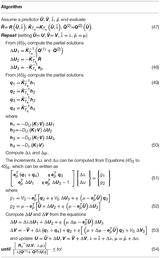
Table 2. Bordering algorithm.

We furnish the expressions of the vectors h_j (j = 1, …, 4), which appear in Equations (50), in the Appendix.

Overall Algorithm for Stability Analysis

We compute the pre-buckling and post-buckling equilibrium paths of a laminated beam by combining the procedures described in Sections Path-Following Procedure and Computation of Stability Points.

More precisely, denoted the initial stiffness matrix by K₀ (see the Appendix) and an arbitrary numeric value by λ₀, we consider the couple λ₀, $U_0={\lambda }_0{K}_0^{-1}{Q}^{(1)}$ as the initial predictor of the first equilibrium state.

We hence correct this predictor as described in section Path-Following Procedure and keep computing equilibrium states along the primary path. We check for the sign of the tangent stiffness matrix determinant in correspondence of each state, which is a simple operation since the solution of the extended system (25) requires the factorization (i.e., the triangular decomposition) of K_T.

If the sign of det K_T changes between two successive states, say i and i + 1, a stability point has passed. We hence switch from the path-following procedure to the procedure for computing stability points.

In particular we assume $\tilde{U}={\text{U}}^{i+1}$, $\tilde{V}=V_0=K_0^{-1}{e}_p$, $\tilde{\lambda }={\lambda }^{i+1}$, $\tilde{\mu }={e_p^T\text{U}}^{i+1}$ (for the meaning of the index p see the beginning of section Computation of Stability Points).

Once the stability point U_c, λ_c has been computed, we check if it is a limit or a bifurcation point. In the case of a limit point we come back to the path-following procedure to complete the primary path. In the case of a bifurcation point, we switch to the secondary (or bifurcated) path by adding to U_c a vector proportional to the eigenvector V

$\begin{array}{cc}U=U_c+\zeta \frac{V}{\Vert V\Vert }& (55)\end{array}$

ζ being a scaling factor to be determined in such a way that it results R(U,λ_c) ≤ tol.

We then follow the secondary path using the path-following procedure and arrest the calculations when the cross-section rotations or the shear strains are more than moderately large or the axial strains are more than infinitesimal (18).

Numerical Results

We present in this section several numerical results relative to the evaluation of the stability points and to the post-buckling behavior of straight and curved beams.

In all the examples we supposed the beam cross-section to be rectangular with lengths H₁ and H₂ along the directions X₁ and X₂, respectively. We denoted the cross-section area by A = H₁H₂, the moments of inertia by I₁ and I₂, the polar moment of inertia by I_G and the De Saint Venant torsional rigidity by J_t

$\begin{array}{cc}{I}_1=\frac{H_1{H}_2^3}{12},I_2=\frac{H_1^3{H}_2}{12},{\text{I}}_{\text{G}}=I_1+I_2,{\text{J}}_{\text{t}}=\frac{H_1^3{H}_2}{3}.& (56)\end{array}$

Concerning the expression of the warping function w, we examined the following three cases:

No Warping (NW): w = 0

Warping Function (W1): w = w₁₁X₁X₂

Warping Function (W3): $w=w_{20}{X}_1^2+w_{11}{X}_1{X}_2+w_{02}{X}_2^2+$

                      $w_{30}{X}_1^3+w_{21}{X}_1^2{X}_2+w_{12}{X_{1}X}_2^3+w_{03}{X}_2^3$.

We used cubic Lagrangian finite elements and a four-point Gauss quadrature formula to compute the tangent stiffness matrix and its derivatives. By this choice we avoided the numerical inconvenient known in literature as shear and membrane (or inplane) locking (see e.g., Prathap and Bhashyam, 1982; Reddy and Averill, 1990).

We always assumed that the external loads retain their directions during the deformation of the beam (dead loading).

Bifurcation Points of Isotropic, Straight and Curved Beams

In order to assess the accuracy of our numerical model, we firstly present some results concerned with bifurcation points of isotropic straight and curved beams. They can be compared with those available in the relevant literature and corresponding to classical beam theories (see e.g., Timoshenko and Gere, 1961; Brush and Almroth, 1975). We assumed a ratio E/G = 0.385 between Young's and shear moduli.

The first example deals with a circular ring submitted to a radial dead load of intensity q, which is uniformly distributed along the centerline. We discretized one half of the ring by 20 finite elements imposing the following boundary conditions (no warping was considered)

$\begin{array}{l}{v}_1=v_2=v_3={\varphi }_1={\varphi }_2={\varphi }_3=0\text{\hspace{1em}for }{X}_3=0,\\ v_1=v_3={\varphi }_1={\varphi }_2={\varphi }_3=0,\text{\hspace{1em}for }{X}_3=\pi R,& (57)\end{array}$

where R is the initial radius of the centerline. In particular, the ratios H₁/H₂ = 2, R/H₂ = 20 were considered.

According to Donnel' s theory (see e.g., Brush and Almroth, 1975), the first bifurcation point occurs at a load level $q_{bif}=4E{I}_1/R^3$ and the buckling mode corresponds to an ovalization of the ring.

It has to be remarked that the first bifurcation point occurs at a sensibly different load level $q_{bif}=3E{I}_1/R^3$ if the external load remains orthogonal to the axis during the deformation of the ring (see e.g., Timoshenko and Gere, 1961; Brush and Almroth, 1975).

Table 3 shows the numerical convergence of the solutions of the extended system (44) for increasing values of the parameter η.

TABLE 3

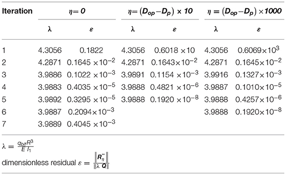
Table 3. Convergence behavior or the first bifurcation point or a circular ring submitted to a radial dead load q uniformly distributed along the centerline (H₁/H₂ = 2, R/H₂ = 20, 20 element mesh).

Denoting by D_p the least diagonal term of the factorized tangent stiffness matrix and by D_op the corresponding term in the factorized initial stiffness matrix K₀, in our numerical experiments we set η = 0, η = (D_op − D_p) × 10 and η = (D_op − D_p) × 1000.

As already observed by Simo and Wriggers (1990), for η = 0 the results exhibit oscillations near the bifurcation point, while for η > 0 they converge in a stable way to the value $3.9888E{I}_1/R^3$.

Table 3 also shows that in the latter case the solution is rather insensitive to the value of η.

The small difference existing between our and Donnel's bifurcation load can be justified observing that Donnel's theory does not account for shear deformation and for the quadratic terms in X₁ and X₂ of the axial strain E₃₃, which are instead present in our model. In all the subsequent numerical applications we η = (D_op − D_p) × 10.

The second example we considered deals with the classical case of a simply supported straight beam loaded by a compressive force at one end (X₃ = L). Table 4 compares the bifurcation loads computed by using the present theory with those corresponding to Euler's theory ($P_{Eul}={\pi }^{2}E{I}_1/L^2$) and Timoshenko's theory, for several the values of the ratio L/H₂, assuming H₁/H₂ = 2. Upon putting ρ = χ P_Eul/GA (χ = 1.2 shear correction factor), we considered both the exact values deriving from Timoshenko's Theory

$\begin{array}{cc}\frac{P_{bif}}{P_{Eul}}=\frac{-\left(4+3\rho \right)+\sqrt{{\left(4+3\rho \right)}^2+16\rho }}{2\rho }& (58)\end{array}$

and the approximate ones (see e.g., Timoshenko and Gere, 1961)

$\begin{array}{cc}\frac{P_{bif}}{P_{Eul}}=\frac{1}{1+\rho }.& (59)\end{array}$

Concerning the comparisons between our and classical theories, we stressed the influences of warping and quadratic terms in X₁, X₂ of the axial strain E₃₃ (Γ terms). It has to be remarked that our theory turns into a first-order shear deformation theory with no shear correction factor (χ = 1) in absence of warping and Γ terms.

TABLE 4

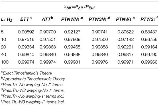
Table 4. First bifurcation load of a simply supported, axially loaded straight beam for several ratios L/H₂ (H₁/H₂ = 2, 20 element mesh).

Table 4 shows that our results corresponding to a cubic warping function and absence of Γ terms closely approximate those by Timoshenko. Furthermore, the influence of Γ terms is found to be appreciable (up to 2.7%) for thick beams. We took into account Γ deformation terms in all the successive numerical applications.

We complete this first group of numerical results by showing some further examples concerned with lateral buckling of straight bars and semicircular arches.

We firstly considered a narrow simply supported beam transversally loaded at the middle point and a narrow cantilever transversally loaded at the free end (H₁/H₂ = 0.1, L/H₂ = 10). The kinematical boundary conditions of the first case are

$\begin{array}{l}{v}_1=v_2=v_3={\varphi }_3=0\text{\hspace{1em}for }{X}_3=0,\\ v_1=v_2={\varphi }_3=0\text{\hspace{1em}for }{X}_3=L,& (60)\end{array}$

Three positions of the load were considered: load at the centroid, load at the extrados (X₁ = 0, X₂ = − H₂/2) and load at the intrados (X₁ = 0, X₂ = H₂/2). The last two cases obviously give rise to a deformation-dependent loading (Q⁽²⁾(U) ≠ 0).

Table 5 shows a comparison between the first bifurcation points computed within the present theory and those corresponding to the classical Prandtl's theory (See e.g., Timoshenko and Gere, 1961).

TABLE 5

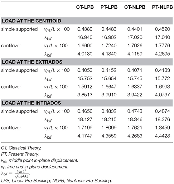
Table 5. First lateral bifurcation point of a simply supported beam loaded by a transverse force Q at the middle point and of a cantilever loaded by a transverse force Q at the free end (H₁/H₂ = 0.1, L/H₂ = 10, 20 element mesh).

In the context of the present theory, we adopted a bilinear warping function (W1) and assumed both a linear and a (geometrically) nonlinear pre-buckling behavior (the first was treated by discarding the part K_L of the tangent stiffness matrix, see the Appendix).

We also generalized Prandtl's theory in order to include a nonlinear pre-buckling behavior. This was obtained by using our model, neglecting shear deformation, warping and Γ terms and making the torsional stiffness equal to GJ_t.

It has to be remarked that the present theory assumes a torsional rigidity equal to GI_G (as in the De Saint Venant theory of torsion without warping) and takes into account warping effects by introducing in the displacement field a polynomial warping function.

It is evident that our numerical results agree better with those by Prandtl when the warping is unconstrained, as in the case of the simply supported beam. On the contrary, in the second example (cantilever), our and Prandtl's results somewhat differ due to the presence of the restraint which doesn't allow the warping of the built-in end.

Further on we remark that the assumption of a linear pre-buckling behavior, as in the original Prandtl's theory, is less accurate for the cantilever than for the simply supported beam. Indeed, in the first case the in-plane displacements are sensibly higher than in the second case and produce moderate rotations.

Finally, Table 6 shows the bifurcation loads of hinged and clamped narrow semicircular arches (v₁ = v₂ = v₃ = ϕ₃ = 0 for X₃ = 0, πR in the first case). The load consists of a uniform radial dead load along the centerline.

TABLE 6

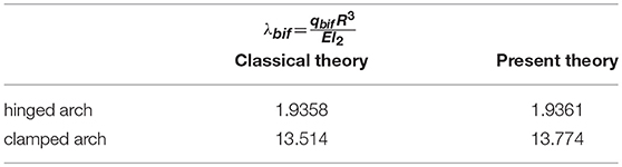
Table 6. First lateral bifurcation load of a hinged and a clamped semicircular arch loaded by a radial dead load q uniformly distributed along the centerline (H₁/H₂ = 0.1, R/H₂ = 10, 20 element mesh).

The results of the present theory are compared with those given in Timoshenko and Gere (1961), which are relative to the classical beam theory. In particular, the first ones correspond to the choice of a bilinear warping function (W1).

Concluding Remarks

This work has developed a finite element model of the moderate rotation theory (MRT) of laminated composite beams proposed in Fraternali et al. (2013), and its application to the computation of nonlinear equilibrium paths and stability points of a variety of numerical examples. The proposed model describes laminated composite beams with arbitrary curvature of the beam axis, and takes into account shear deformation, warping effects, in-plane and out-of-plane instability. For the straight and curved beams examples analyzed in the present study, we conclude the following:

(i) the moderate rotation theory (MRT) and the classical beams theories correlate very well in almost all isotropic cases;

(ii) the influence of warping effects on the bifurcation load is generally pretty high for beams made up of composite materials.

Future work will apply the model presented in this work to a wide collection of technically relevant case-studies, with special emphasis on the study of the stability of light-weight roof structures and arch bridges, which make use of laminated composite beams (Fraternali et al., 2013).

Author Contributions

IM led the numerical part of the study. MM supervised the numerical part of the study. AA led the mechanical modeling part of the study. FF supervised all tasks.

Conflict of Interest Statement

The authors declare that the research was conducted in the absence of any commercial or financial relationships that could be construed as a potential conflict of interest.

Acknowledgments

IM, AA, and FF gratefully acknowledge financial support from the Italian Ministry of Education, University and Research (MIUR) under the Departments of Excellence grant L.232/2016.

Supplementary Material

The Supplementary Material for this article can be found online at: https://www.frontiersin.org/articles/10.3389/fbuil.2018.00057/full#supplementary-material

References

Ascione, L., Berardi, V. P., Giordano, A., and Spadea, S. (2013). Local buckling behavior of FRP thin-walled beams: a mechanical model. Comp Struct. 98, 111–120. doi: 10.1016/j.compstruct.2012.10.049

CrossRef Full Text | Google Scholar

Ascione, L., Giordano, A., and Spadea, S. (2011). Lateral buckling of pultruded FRP beams. Compos B Eng. 42, 819–824. doi: 10.1016/j.compositesb.2011.01.015

CrossRef Full Text | Google Scholar

Bathoz, I. L., and Dhatt, G. (1979). Incremental displacement algorithms for non-linear problems. Int. J. Num. Meth. Engng. 14, 1262–1267. doi: 10.1002/nme.1620140811

CrossRef Full Text | Google Scholar

Bencardino, F., Rizzuti, L., Spadea, G., and Swamy, R. N. (2012). Implications of test methodology on post-cracking and fracture behavior of steel fibre reinforced concrete. Compos. B Eng. 46, 31–38. doi: 10.1016/j.compositesb.2012.10.016

CrossRef Full Text

Brush, D. O., and Almroth, B. O. (1975). Buckling of Bars, Plates and Shells. New York, NY: McGraw-Hill.

Budiansky, B. (1974). “Theory of buckling and post-buckling behavior of elastic structures,” in Advances in Applied Mechanics, eds Chia-Shun Yih (New York, NY: Academic Press), 1–65.

Google Scholar

Feo, L., and Fraternali, F. (2000). On a moderate rotation theory of thin-walled composite beams. Compos. B. Eng. 31, 141–158. doi: 10.1016/S1359-8368(99)00079-7

CrossRef Full Text | Google Scholar

Feo, L., and Mancusi, G. (2010). Modeling shear deformability of thin-walled composite beams with open cross-section. Mech. Res. Commun. 37, 320–325. doi: 10.1016/j.mechrescom.2010.02.005

CrossRef Full Text | Google Scholar

Fraternali, F. (2007). Free discontinuity finite element models in two-dimensions for in-plane crack problems. Theor. Appl. Fract. Mech. 47, 274–282. doi: 10.1016/j.tafmec.2007.01.006

CrossRef Full Text | Google Scholar

Fraternali, F., Angelillo, M., and Fortunato, A. (2002). A lumped stress method for plane elastic problems and the discrete-continuum approximation. Int. J. Solids Struct. 39, 6211–6240. doi: 10.1016/S0020-7683(02)00472-9

CrossRef Full Text | Google Scholar

Fraternali, F., Ciancia, V., Chechile, R., Rizzano, G., and Feo, L. (2011). Incarnato, L. Experimental study of the thermo-mechanical properties of recycled PET fiber reinforced concrete. Comp. Struct. 93, 2368–2374. doi: 10.1016/j.compstruct.2011.03.025

CrossRef Full Text | Google Scholar

Fraternali, F., Farina, I., Polzone, C., Pagliuca, E., and Feo, L. (2012). On the use of R-PET strips for the reinforcement of cement mortars. Compos. B. Eng. 46, 207–210. doi: 10.1016/j.compositesb.2012.09.070

CrossRef Full Text | Google Scholar

Fraternali, F., Negri, M., and Ortiz, M. (2010). On the convergence of 3D free discontinuity models in variational fracture. Int. J. Fract. 166, 3–11. doi: 10.1007/s10704-010-9462-0

CrossRef Full Text | Google Scholar

Fraternali, F., Spadea, S., and Ascione, L. (2013). Buckling behavior of curved composite beams with different elastic response in tension and compression. Compos. Struct. 100, 280–289, doi: 10.1016/j.compstruct.2012.12.021

CrossRef Full Text | Google Scholar

Keller, H. B. (1977). “Numerical solution of bifurcation and nonlinear eigenvalue problems,” in Applications of Bifurcation Theory, eds P.H. Rabinowitz (New York, NY: Academic Press), 359–384.

Google Scholar

Markkula, S., Malecki, H. C., and Zupan, M. (2013). Uniaxial tension and compression characterization of hybrid CNS-glass fiber-epoxy composites. Comp. Struct. 95, 337–345. doi: 10.1016/j.compstruct.2012.07.013

CrossRef Full Text | Google Scholar

Mascolo, I., Fulgione, M., and Pasquino, M (in press). Lateral torsional buckling of compressed open thin walled beams: experimental confermations. Int. J. Mansory Res. Innovat.

Mascolo, I., and Pasquino, M. (2016). Lateral-torsional buckling of compressed highly variable cross section beams. Curved. Al. Layer. Struct. 3443, 146–153. doi: 10.1515/cls-2016-0012

CrossRef Full Text | Google Scholar

Nomizu, K., and Kobayashi, S. (1963). Foundations of Differential Geometry. New York, NY: Wiley.

Google Scholar

Özütok, A., and Madenci, E. (2017). Static analysis of laminated composite beams based on higher-order shear deformation theory by using mixed-type finite element method. Int. J. Mech. Sci. 130, 234–243. doi: 10.1016/j.ijmecsci.2017.06.013

CrossRef Full Text | Google Scholar

Prathap, G., and Bhashyam, G. (1982). Reduced integration and the shear-flexible beam element. lnt.J. Num. Meth. Engng. 18, 195–210. doi: 10.1002/nme.1620180205

CrossRef Full Text | Google Scholar

Reddy, J. N. (1992). An Introduction to the Finite Element Method, 2nd Edn. New York, NY: McGraw-Hill.

Google Scholar

Reddy, J. N., and Averill, R. C. (1990). On the behavior of plate elements based on the first-order shear deformation theory. Engng. Comput. 7, 57–74. doi: 10.1108/eb023794

CrossRef Full Text | Google Scholar

Riks, E. (1972). The application of newton's method to the problem of elastic stability. J. Appl. Mech. 39, 1060–1066. doi: 10.1115/1.3422829

CrossRef Full Text | Google Scholar

Roberts, T. M., and Al-Ubaidi, H. (2001). Influence of shear deformation on restrained torsional warping of pultruded FRP bars of open cross-section. Thin-Walled Struct. 39, 395–414. doi: 10.1016/S0263-8231(01)00009-X

CrossRef Full Text | Google Scholar

Schmidt, B., Fraternali, F., and Ortiz, M. (2009). Eigenfracture: an eigendeformation approach to variational fracture. Siam. J. Multiscale Model. Simul. 7, 1237–1266. doi: 10.1137/080712568

CrossRef Full Text | Google Scholar

Simo, J. C., and Wriggers, P. (1990). A general procedure for the direct computation of turning and bifurcation points. int. J. Num. Meth. Engng. 30, 155–176. doi: 10.1002/nme.1620300110

CrossRef Full Text | Google Scholar

Spence, A., and Jepson, A. D. (1985). Folds in the solution of two parameter systems and their calculation, Pan. I, SIAM J. Num. Anal. 22, 347–368. doi: 10.1137/0722021

CrossRef Full Text | Google Scholar

Timoshenko, S. P., and Gere, J. M. (1961). Theory of Elastic Stability. New York, NY: McGraw-Hill.

Google Scholar

Trefftz, E. (1930). “Über die Ableitung der Stäbilitats-kriterien des elastischen Gleichgewichtes aus der elasticitäts theorie endlicher Deformationen,” in Proceedings of the Third international Congress for Applied Mechanics (Stockholm), 44–50.

Viera, R. F., Virtuoso, F. B. E., and Pereira, E. B. R. (2013). A higher order thin-walled beam model including warping and shear modes. Int. J. Mech. Sci. 66, 67–82. doi: 10.1016/j.ijmecsci.2012.10.009

CrossRef Full Text | Google Scholar

Notation

We report below the list of the main notations used in the text. Throughout this paper we use boldface character to denote numerical vectors and matrices; we also use the superscript T to denote the transpose of a vector or a matrix.

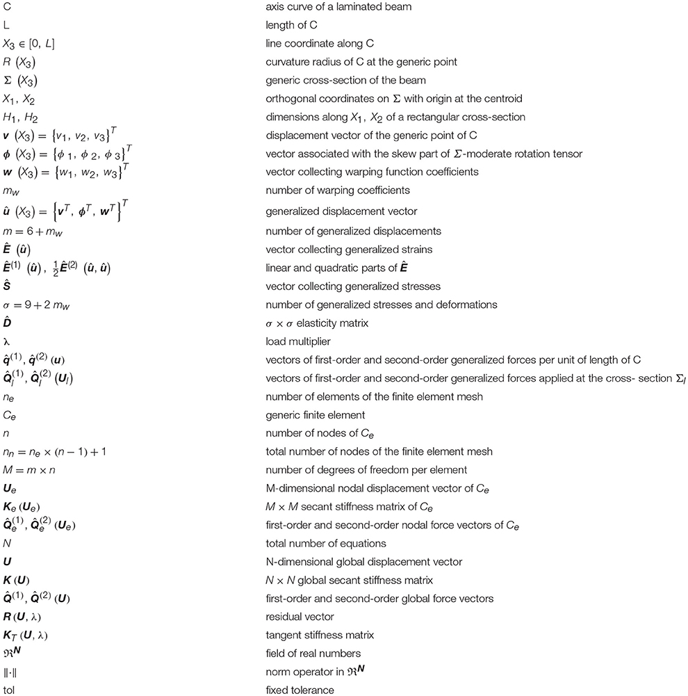
Given a scalar function f(U,λ):ℜ^N×ℜ → ℜ, we denote by D_Uf the vector which represents the Gateaux derivative of f with respect to U

$V^T{D}_{U}F={\text{lim}}_{\gamma \to 0}\frac{1}{\gamma }\left[f\left(U+\gamma V,\lambda \right)-f\left(U,\lambda \right)\right],\forall V\in {\Re }^N$

and by D_λf the partial derivative of f with respect to λ.

Similarly, given a vector function R(U,λ):ℜ^N×ℜ → ℜ^N, we denote by D_UR the N × N matrix which represents the Gateaux derivative of R with respect to U

$D_{U}RV={\lim }_{\gamma \to 0}\frac{1}{\gamma }\left[R\left(U+\gamma V,\lambda \right)-R\left(U,\lambda \right)\right],\forall V\in {\Re }^N,$

and by D_λR the partial derivative of R with respect to λ.

Finally, in the case of a scalar function f(U, λ), we denote by $D_U^{2}f$ the bilinear operator $D_U^{2}f{V}_1{V}_2=V_2^T{D}_U\left(D_{U}f\right)V_1,\forall V_1,V_2\in {\Re }^N.$