Manifold Learning and Clustering for Automated Phase Identification and Alignment in Data Driven Modeling of Batch Processes

Introduction

Most commercial APIs are produced by consecutive batch operations that follow a pre-established recipe. Likewise, these operations are run as the sequence of multiple process phases in single units. The flexibility provided on the duration of most of these phases results in batches that follow similar trajectories but with uneven duration. Fed-batch fermentation, complex reaction sequences followed by crystallization, centrifugation, and drying are some examples of the type of processes found in the pharmaceutical industry. In recent years, the increasing interest in having better control of these processes together with the increasing availability of process analytical technologies (PAT) has driven the application of data driven modeling for process monitoring, quality prediction, and control (García-Muñoz and Mercado, 2013; Yu et al., 2014; Debevec et al., 2018). However, irrespective of the modeling approach, building models that capture meaningful variability of the processes and which are not limited to describe individual process phases requires the identification and alignment of the various phases. In general, methods that do not consider the steps for phase identification and batch alignment, are less robust in dealing with data coming from multi-phase, uneven processes. González-Martínez et al. (2014) demonstrate that the methods which do not synchronize key events of the batch process diminish the performance of the data driven models. In most cases, these methods rely on unfolding the data in the variable-wise direction. This eliminates the practical need for aligning batches of uneven duration and can deal with non-aligned data to a certain extent (Facco et al., 2009; Wold et al., 2009; Mingxing et al., 2010). The observation-wise unfolding-T scores batch-wise unfolding (OWU-TBWU) (Wold et al., 2009) is an example of these types of methods. It is widely considered as the default pre-treatment step for batch data of uneven duration. In OWU-TBWU, variable-wise unfolding is applied to train a Partial Least Squares (PLS) model that links the unfolded data with a dummy time-batch progression variable. The data is then interpolated based on the PLS T-scores and finally, batch-wise unfolding is applied to the interpolated data. The interpolation procedure applied as part of OWU-TBWU is known as TLEC (González-Martínez et al., 2014). In most cases, these methods have been demonstrated in simple benchmark processes that normally would not require phase identification however its applicability to real industrial scenarios is limited to individual process phases that must be manually isolated from the rest of the process.

One of the most intuitive ways to identify different phases in a process is determining the time when the events that mark the phase change occur. In principle, this information can be extracted from the data in the form of distinctive events on the trajectories of certain process variables. Doan and Srinivasan (2008) propose the automated identification of Singular Points (SP) in the data as a method to denote when the phase change takes place. Different methods have been proposed to identify SP directly from data trajectories. Srinivasan and Qian (2005) use numerical strategies based on the definition of three different types of SP that can occur in a given process, i.e., 1) extremes, 2) sharp changes or discontinuities, and 3) trend changes. Thus, according to this method, the identification of SP in the signal is based on ad-hoc thresholds defined for 1) signal changes over time, 2) numerically approximated first and second derivatives, and 3) the regression analysis of linear models. Alternatively, Kaistha and Moore (2001) proposed the use of signal filters to extract the event times from the trajectories, however this requires the a priori definition of the features to be used as signal filters. Maurya et al. (2007) use an approach equivalent to dynamic trend analysis were the data trajectories are halved sequentially to identify trends based on the fitness of polynomials of up to second degree. Once the trends are identified, the SP are defined as the changing time between trends, and a fuzzy-matching-based method is used to estimate similarity of new trajectories with the identified trends. Although these approaches are very intuitive, it is difficult to generalize and to automate their application to different processes, because they require the definition and tuning of ad-hoc strategies. Additionally, only univariate changes are used as source of information on the process phases and some of the strategies can be highly sensitive to noise in the signals.

More advanced methods which consider automated phase identification are divided into two groups: either based on clustering analysis or model identification (Wang et al., 2018). Approaches based on clustering analysis can perform supervised or unsupervised learning (i.e., imposing the knowledge on the number or the type of expected process phases, or using methods which aim to learn the existence of different phases directly from the data). In the adjoined multi-model approach for monitoring, proposed by Ng and Srinivasan (2009), a fuzzy C-means algorithm for clustering is used to determine the membership grade of every data point in the space of the process variables. Overlapping PCA models are trained to deal with points that share membership between consecutive process phases. Wang et al. (2018) implement a sequential clustering approach with an ad-hoc index defined to evaluate the goodness of the phase partition. A support vector data description method is then proposed to classify new data. Zhang et al. (2018) use a standard implementation of K-nearest neighbor for clustering on the space produced by a moving window Principal Component Analysis (PCA). Luo et al. (2016) propose the warped k-means method to identify clusters directly on the time series trajectories of the selected variables. The main limitation of these methods is the space on which the clustering analysis is performed. The use of PCA based latent space or the space of the process variables, significantly reduces the ability to identify clusters for the different phases of the process.

Methods based on model identification explore formulations based on the fitness of a given model to a period of the time series and the transition to a different model when a change in phase occurs. PCA or extensions of this method are commonly used as modeling strategy. The goal is to identify a model from the data and to establish a method to determine when the data deviates from the model. The deviation is then an indication of change on the process phase. Qiao et al. (2012) and Sun et al. (2011) propose PCA based model identification strategies and define statistical parameters as the cumulative contributions between different PCA models to identify the phase change. Liu et al. (2016) implement a similar approach based on kernel-PCA. This method can deal with non-linear relations in the data. More recently Wang et al. (2019) propose a combined approach between model identification and cluster analysis. A linear dynamic model is first identified and then distances are computed between the trajectories of different batches to apply cluster analysis. K-means was used to identify clusters in the distance data. Beaver et al. (2007) use non-hierarchical k-PCA as way to find an optimal separation of phases by finding the best set of PCA models to fit a given set of process windows in the time series. Thus, the final optimal solution will provide the partition points as well as the number of process phases. Zhu et al. (2011) present a more robust method based also on process windows in the time series, but in this case, a coupled Independent component analysis (ICA) and PCA model are fitted to the lagged data of each window. The lagged data is selected based on the number of phases in the process, multiple alternatives of phase separation are implemented and a final assembled model is constructed by aggregating solutions from different alternatives on the number and location of the clusters. Finally, other methods that do not require model identification or cluster analysis have been also proposed, e.g., Guo and Jin (2019) propose a method for phase identification based on the changes in the correlation matrix of a moving window of operation.

Most methods for batch alignment are based on time interpolation for compression/expansion of the time trends. This transformation is applied following different approaches: 1) the direct interpolation from start to end, 2) the use of an indicator variable, and 3) the dynamic time warping DTW (Kassidas et al., 1998). Although DTW can be very effective to synchronize two or more time series, it suffers of some drawbacks that limit its applicability significantly. DTW can not be applied for online monitoring, it is computational expensive and the shrinking/expansion effect on the time trend might result in distorting the information contained in the data (Guo and Jin, 2019). Solutions to the distortion problem have been proposed based on the combination of global and local constraints to the distance optimization that is solved in DTW (Spooner et al., 2017; Zhang et al., 2017). However, the complexity of the problem that needs to be solved increases and a single generic strategy that will guarantee non-aggressive and non-pathological warping in every case does not exist.

This paper presents a novel method based on machine learning algorithms for phase identification and alignment. The proposed approach combines unsupervised and supervised learning strategies and exploits the principles of manifold learning to reduce the dimensionality of the space that contains information about the phase changes in the process. First, t-SNE is used to embed the data on a reduced space where the process phases can be identified more easily. Then, SVMs are used to model the manifold learning performed by t-SNE. A similar approach, known as inductive manifold learning, has been proposed in applications of partner recognition Kim and Lee (2014). In the second stage of the method, supervised learning based on SVMs is applied to classify the process condition at every time point and determine its membership to the corresponding phase. Batch alignment is achieved through the sequential alignment of the individual process phases. The time progression of every phase is sub-sampled at a constant frequency using linear interpolation to guarantee that every phase has the same duration in all batches. Some of the advantages of this method compared to other approaches are: 1) it performs unsupervised phase identification, therefore it does not require pre-defining the number of phases or the events that indicate phase changes. 2) It works for processes with uneven phase duration. 3) It accounts and exploits the sequential nature of the phases in the process. 4) It results in a very intuitive visualization of the phases of the process and allows for an early identification of deviations in the process. 5) It is a low complexity method with very low computational requirements for online implementation. 6) As opposed to other approaches based on PCA, it does not make assumptions on linearity and normality of the data. 7) Only two elements must be defined for the algorithm to work, i.e., the variables used for phase identification and the perplexity parameter of the t-SNE algorithm. 8) Distortion in the time progression is not induced because the data is interpolated from the start to end of every phase at constant frequency. The effectiveness of this method is demonstrated not only on a in-silico benchmark case (i.e., the Pensim process), but also on two real industrially relevant cases based on data obtained from the large scale production of APIs.

The first part of this paper provides a background on the methods used in the proposed algorithm, i.e., t-SNE and SVMs for regression and classification. Then the proposed method is explained, supported by the results obtained from its application to the Pensim benchmark case study. The results section discusses the application of the proposed method to the industrial cases. Data from a hydrogenation reaction and the operation of a centrifuge-dryer is evaluated to determine the performance of the method in real process data. Finally, the conclusions summarize the main findings of this work.

Methods

This section provides background on the machine learning algorithms used as part of the proposed method for automated batch identification and alignment. The main aspects of the t-SNE method and SVMs are discussed. For further insight into these methods, the reader is directed to the cited references.

t-Distributed Stochastic Neighbour Embedding

t-Distributed Stochastic Neighbour Embedding developed by Van der Maaten and Hinton (2008) is a non-linear dimensionality reduction algorithm that has proven to be very effective for visualization of high dimensional data (Van der Maaten, 2014; Kobak and Berens, 2018). Three main aspects of t-SNE can be highlighted when it is compared with PCA. PCA is used as reference because it is a widely applied method for dimensionality reduction in applications of phase identification and in general in data driven modeling. First, PCA aims to keep in the low dimensional space the directions of largest variability while t-SNE goal is to keep the local similarities and as result magnifies differences between data points. Secondly, PCA’s reduced space results from the linear combinations of the input space while t-SNE is a non-parametric manifold learning method for which does not exist an explicit mathematical form of the reduced space and for which does not exist an inverse form. Finally, PCA can be obtained via singular value decomposition and the dimensionality reduction is limited by the linear correlations found in the input space, t-SNE dimensionality reduction results from minimizing the Kullback-Leibler (KL) divergence over all data points, an normally a bi-dimensional or tri-dimensional space is selected as output to allow visualization of embedded data. The use of t-SNE for applications in data driven modeling has being investigated in very recent years, however the focus has been limited to visualization and fault identification (Zhu et al., 2019; Zheng and Zhao, 2020). In this work, t-SNE was chosen because the mentioned characteristics of the method fit well with the requirements of the application for process phase identification. The goal is to identify similarities between data points belonging to the same process phase. There is not a priori knowledge on the distribution of the data, nor on the type of correlations present. The dimensionality of the reduced space is kept low and it is non-dependent of the case.

Conceptually t-SNE aims to find the distribution of data points in the reduced space that retains most of the original local similarities between data points in the high dimensional input space. t-SNE was proposed as a modification to the original Stochastic Neighbor Embedding (SNE) by Hinton and Roweis (2002). In SNE the conditional probability, $p_{j|i}$, for the similarity of point ${\mathit{x}}_j$ respect to point ${\mathit{x}}_i$, based on the Euclidean distance in the original high dimensional space, is given by Eq. 1.

$p_{j|i}=\frac{exp\left(-{\Vert {\mathit{x}}_i-{\mathit{x}}_j\Vert }^2/2{\sigma }_i^2\right)}{{{\displaystyle \sum }}_{k\ne i}exp\left(-{\Vert {\mathit{x}}_i-{\mathit{x}}_k\Vert }^2/2{\sigma }_i^2\right)}(1)$

This conditional probability is high for neighboring points, very low for distant points, and follows a Gaussian distribution centered at ${\mathit{x}}_i$ with variance ${\sigma }_i$. The value assigned for ${\sigma }_i$ in the SNE method is determined based on the perplexity parameter $Perp\left(P_i\right)$ which is the main tuning parameter of the method and needs to be defined by the user depending on the application. The perplexity can be interpreted as a measure for the expected number of neighbors and it is related with the probability distribution $P_i\sim \mathcal{N}\left({\mathit{x}}_i,{\sigma }_i\right)$ through the Shannon entropy of $P_i$ according to Eq. 2 (Van der Maaten and Hinton, 2008). Binary search methods or root-finding methods can be used to determine the values of ${\sigma }_i$. These solutions should make the perplexity of the obtained probability distributions match the value specified by the user (Van der Maaten, 2014).

$Perp\left(P_i\right)=2^{-{\displaystyle {\sum }_j{p}_{j|i}{\text{log}}_2{p}_{j|i}}}(2)$

For t-SNE a symmetric function is used to describe the similarities in the high dimensional space. This is achieved by using the joint probability $p_{ij}$ given by Eq. 3 where N is the number of data points. In t-SNE the similarities between points in the low dimensional space are described using a normalized t-distribution with one degree of freedom instead of the Gaussian distribution used in the original SNE. This reduces the crowding of the embedded points in the low dimensional space because the heavier tails of the t-distribution make that dissimilar points in the input space to be embedded farther apart in the low dimensional map. This results in creating more space to distribute the locally similar points (Van der Maaten, 2014). The joint probability $q_{ij}$ for the two points, ${\mathit{y}}_i$ and ${\mathit{y}}_j$, embedded in the low dimensional space is given by Eq. 4.

$p_{ij}=\frac{p_{i|j}+p_{j|i}}{2N}(3)$

$q_{ij}=\frac{{\left(1+{\left|\left|{\mathit{y}}_i-{\mathit{y}}_j\right|\right|}^2\right)}^{-1}}{{{\displaystyle \sum }}_{k\ne l}{\left(1+{\Vert {\mathit{y}}_k-{\mathit{y}}_l\Vert }^2\right)}^{-1}}(4)$

The manifold learning in t-SNE is achieved via the minimization of the loss function. This loss function is the KL divergence between the joint probabilities of the points in the low-dimensional space $\left(q_{ij}\right)$ and the input high dimensional space $\left(p_{ij}\right)$ according to Eq. 5.

$\mathrm{ℒ}={\displaystyle \sum }_{i,j}{p}_{ij}{\text{log}}_2\frac{p_{ij}}{q_{ij}}(5)$

Minimizing the KL divergence results in finding the location for the N data points in the low dimensional space that keeps the similarities between points as close as possible to the originals. The exact solution of this optimization problem can be obtained applying descent methods using the analytical gradient of the KL divergence shown in Eq. 6. Since the solution of this problem is $\mathcal{O}\left(N^2\right)$ the memory requirements can become too large when the number of data points in the data set is large. To solve this issue the t-SNE method can be applied based on the Barnes-Hut approximation. The reader is referred to Van der Maaten (2014) for further details on the derivation of this approximation.

$\frac{\partial \mathbf{ℒ}}{\partial {\mathit{y}}_i}=4{\displaystyle \sum }_{i,j}\left(p_{ij}-q_{ij}\right)q_{ij}\frac{\left({\mathit{y}}_i-{\mathit{y}}_j\right)}{{{\displaystyle \sum }}_{k\ne l}\left(1+{\Vert {\mathit{y}}_k-{\mathit{y}}_l\Vert }^2\right)}(6)$

Finally, the manifold learning obtained via t-SNE is non-parametric, this means that it can not be inverted and can not be applied to embed new data points in an already existing low dimensional space. This limits significantly the application of this method. A solution already proposed is to parameterize the t-SNE manifold learning with the parallel application of a machine learning method for regression. Van der Maaten (2009) propose the use of artificial neural networks (ANN) for this purpose. This approach has been already tested in different applications, however tuning the ANN to reproduce the manifold learning is rather complex task with many degrees of freedom. Zhu et al. (2019) propose an algorithm to implement this approach in the visualization of process data through parametric t-SNE. In this paper an alternative approach is implemented based on SVM for regression. Thus, the manifold learning obtained via t-SNE is approximated via SVMs. A similar approach has been already proposed to perform pattern recognition (Kim and Lee, 2014). This approach is preferred because the degrees of freedom on the SVMs are lower than those of an ANN, making the implementation more robust and reproducible. The accuracy achieved via SVM on the manifold learning proved to be sufficient for the intended application in the three cases evaluated in this work.

Support Vector Machines

The proposed algorithm for phase identification of batch processes exploits SVMs for two different purposes. First, a non-linear regression model is trained to reproduce the manifold learning obtained via t-SNE. Secondly, binary classification models are trained to assign the membership of the new data points to each of the identified process phases. In this section some concepts on the use of SVMs for regression and classification are introduced.

The working principle of an SVM is to define an hyperplane in a high dimensional feature space $\left(\mathrm{ℱ}\subseteq {\mathrm{ℝ}}^{{\mathrm{n}}_{\mathrm{f}}}\right)$ which, 1) for the classification problem discriminates the data or 2) for the regression problem best describes the response in terms of the predictors. This hyperplane is defined in terms of the support vectors which are a subset of data points on every side of the hyperplane in the feature space. If $\phi :{\mathit{ℝ}}^{n_{\mathrm{i}}}\to \mathrm{ℱ}$ is the mapping function between the input space where the data points are initially located $\left(\mathit{x}\in {\mathrm{ℝ}}^{{\mathrm{n}}_{\mathrm{i}}}\right)$ and the feature space, a linear hyperplane is defined as shown in Eq. 7.

$f\left(\mathit{x}\right)={\mathit{w}}^T\phi \left(\mathit{x}\right)+b:\left(\mathit{w},\phi \right)\in {\mathrm{ℝ}}^{{\mathrm{n}}_{\mathrm{f}}},b\in \mathrm{ℝ}(7)$

However, determining the location of the hyperplane in terms of w and b does not require $\phi \left(\mathit{x}\right)$ to be evaluated explicitly. Instead, the inner product in the feature space $\phi {\left({\mathit{x}}_i\right)}^T\phi \left({\mathit{x}}_j\right)$ can be replaced by the kernel function $K\left({\mathit{x}}_i,{\mathit{x}}_j\right)$ (Aizerman et al., 1964). This results from the application of the Mercer’s condition (James and Russell, 1909). The training method for SVMs is derived from the primal and dual formulation of the optimization problem, which is different for classification and regression. The binary classification problem considers the output to be a class variable $y_i\in \left\{-\mathrm{1,1}\right\}$ and the equation of the hyperplane to be $f\left(\mathit{x}\right)=0$ for all points lying in the hyperplane. Thus, the problem of finding the best discriminating hyperplane is to determine the values of w and b that maximize the margin, i.e., the distance from the hyperplane to the support vectors. This problem is equivalent to minimizing the L2-norm $\Vert \mathit{w}\Vert$ subject to the condition that for all the training data points $y_{i}f\left({\mathit{x}}_i\right)\ge 1$ with the support vectors being located in the boundary where $y_{k}f\left({\mathit{x}}_k\right)=1$. The Lagrangian for the primal formulation of the optimization problem for classification is given in Eq. 8, where ${\alpha }_i$ are the multipliers.

${\mathcal{J}}_P=\frac{1}{2}\left({\mathit{w}}^{\mathit{T}}\mathit{w}\right)-{\displaystyle \sum }_i{\alpha }_i\left(y_{i}f\left({\mathit{x}}_i\right)-1\right)(8)$

The dual formulation in Eq. 9 results from introducing the optimality conditions and replacing the inner product in the feature space by the kernel function. The solution to this optimization problem results in the formulation of the classification hyperplane as $f\left(\mathit{x}\right)={\displaystyle {\sum }_i{\alpha }_i^{\text{*}}{y}_{i}K\left(\mathit{x},{\mathit{x}}_i\right)+{\mathit{b}}^{\text{*}}}$ (Burges, 1998), where ${\alpha }^{\text{*}}$ and $b^{\text{*}}$ are the optimal solutions for the Lagrangian multipliers and the intercept, respectively.

$\begin{array}{ll}\underset{\mathit{\alpha }}{\text{max}}\hfill & {\displaystyle \sum }_i{\alpha }_i-\frac{1}{2}{\displaystyle \sum }_i{\displaystyle \sum }_j{\alpha }_i{\alpha }_j{y}_i{y}_{j}K\left({\mathit{x}}_i,{\mathit{x}}_j\right)\hfill \\ \text{s}.\text{t}.\hfill & {\displaystyle \sum }_i{\alpha }_i{y}_i=0\hfill \end{array}(9)$

Equation 10 shows the regularized optimization problem for a regression problem. The loss function in this case is defined based on an e-intensive loss function according to the original formulation of the SVM problem by Vapnik et al. (1996). In this case the output $y_i$ is a continuous response variable and the intensive loss function equals zero if $|y_i-f\left({\mathit{x}}_i\right)|\le \epsilon$, otherwise it takes the value of $|y_i-f\left({\mathit{x}}_i\right)|-\epsilon$.

$\begin{array}{cc}\underset{\mathit{w},b}{\text{min}}& \frac{1}{N}{\displaystyle \sum }_i|y_i-f\left({\mathit{x}}_i\right){|}_{\epsilon }+\frac{\lambda }{2}{\left|\left|\mathit{w}\right|\right|}^2\end{array}(10)$

The primal formulation for this regression problem is given in Eq. 11. ${\mathrm{ℰ}}_i,{\mathrm{ℰ}}_i^{\prime }$ are the slack variables which allow violation of the error margin around the regression hyperplane and the constant $c>0$ establishes an overall tolerance for these violations.

$\begin{array}{ll}\underset{\mathit{w},b,\mathrm{ℰ},{\mathrm{ℰ}}^{\text{*}}}{\text{min}}\hfill & \frac{1}{2}\left({\mathit{w}}^T\mathit{w}\right)+c{\displaystyle \sum }_i\left({\mathrm{ℰ}}_i+{\mathrm{ℰ}}_i^{\prime }\right)\hfill \\ \text{s}.\text{t}.\hfill & y_i-f\left({\mathit{x}}_i\right)\le \epsilon +{\mathrm{ℰ}}_i\hfill \\ \hfill & f\left({\mathit{x}}_i\right)-y_i\le \epsilon +{\mathrm{ℰ}}_i^{\prime }\hfill \\ \hfill & {\mathrm{ℰ}}_i,{\mathrm{ℰ}}_i^{\prime }\ge 0\hfill \end{array}(11)$

As in the case of the classification problem, the dual formulation allows to find the solution without the need for computing the inner product explicitly in the feature space. Equation 12 presents the dual formulation obtained from the Lagrangian, the optimality conditions and the kernel function. The solution of this problem results in the dual representation of the regression model $f\left(\mathit{x}\right)={\displaystyle {\sum }_i\left({\alpha }_i^{*}-{\alpha }_i^{\prime *}\right)K\left(\mathit{x},{\mathit{x}}_i\right)+b^{\text{*}}}$ (Suykens et al., 2002).

$\begin{array}{ll}\underset{\mathit{\alpha },{\mathit{\alpha }}^{\prime }}{\text{max}}\hfill & -\frac{1}{2}{\displaystyle \sum }_{i,j}\left({\alpha }_i-{\alpha }_i^{\prime }\right)\left({\alpha }_j-{\alpha }_j^{\prime }\right)K\left({\mathit{x}}_i,{\mathit{x}}_j\right)\hfill \\ \hfill & -\epsilon {\displaystyle \sum }_i\left({\alpha }_i-{\alpha }_i^{\prime }\right)+{\displaystyle \sum }_i{y}_i\left({\alpha }_i-{\alpha }_i^{\prime }\right)\hfill \\ \text{s}.\text{t}.\hfill & {\displaystyle \sum }_i\left({\alpha }_i-{\alpha }_i^{\prime }\right)=0\hfill \\ \hfill & {\alpha }_i,{\alpha }_i^{\prime }\in [0,c]\hfill \end{array}(12)$

Zhang and Song (2015) discuss several different kernel functions. The method proposed in this paper uses the kernel of a Gaussian Radial Basis Function (RBF) for classification and regression. The RBF kernel $K\left({\mathit{x}}_i,{\mathit{x}}_j\right)=exp\left(-\gamma {\Vert {\mathit{x}}_i-{\mathit{x}}_j\Vert }^2\right)$ has proven to be successful in many applications, the model fitness can be tuned via γ to guarantee accuracy and prevent overfitting.

Automated Phase Identification and Alignment for Batch Processes

Overview

The proposed algorithm for automated identification and alignment of phases in batch processes consists of three stages. The main input required for the algorithm is a set of training data, i.e., a given set of historical batches that display the normal operation of the process. The user must define one batch to be the reference batch and the set of variables to be used by the method to learn information on the phases of the process. Ideally these variables should display the changes that are associated with the different phases of the process. Once these inputs have been defined the first stage of the algorithm will result in the unsupervised identification of the process phases. The information obtained from this stage consists of the reference time points in time series of the reference batch used for phase identification and the embedded map where clusters are formed by data points of every identified phase. In the following stage these elements are used to train the machine learning method which is the core for the phase identification and alignment of the future batches. This method consists of two consecutive SVMs. First, a regression model which is trained to reproduce the manifold learning obtained by t-SNE and then a set of SVM models for binary classification that are trained to assign the membership of every new data point to the corresponding phase of the process. Thus, the second stage results in the models that will be used for the implementation of the algorithm to new batches. The final stage is the online application of the method for batch alignment. This stage consists of the application of the already trained SVM models following a simple programmed sequential logic to assign the phase membership to the new data points. Figure 1 shows the information flow through the different stages of the algorithm. Every stage of the proposed method is now explained in detail.

FIGURE 1

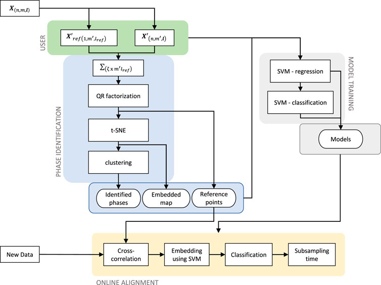
FIGURE 1. Architecture of the method for automated phase identification and alignment.

In-silico data generated from the Pensim benchmark case is used in this section to demonstrate the results obtained through the application of the proposed method. Pensim is a model for the industrial scale production of penicillin (Birol et al., 2002). The process data was obtained from simulations of the Pensim model implemented in RAYMOND (Gins et al., 2014).

Phase Identification

Batch process data obtained from online sensors which is sequentially concatenated every time that a new batch is produced is depicted as a 3-way data array or tensor. represents a training set that consists of the data stored from n historical batches, for which m variables were continuously measured for a given l number of time instances. Since every batch can have a different duration, l is a vector with the number of time instances per batch as individual elements. This means that the tensor X consist of n horizontal slices of data with different lengths as shown in Figure 2. This figure also shows the batch-wise unfolded version of X to illustrate how the batch data normally consists of several uneven sets of equivalent data. Every set represents a phase in the process.

FIGURE 2

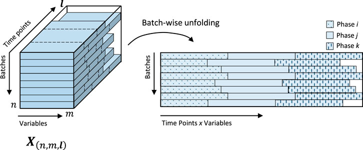
FIGURE 2. Data structure in multi-phase batch processes.

As shown in Figure 1 the method takes X as input. Out of this data, the user must define first the reference batch and the subset of $m^{\prime }\le m$ variables which are informative with respect to phase changes in the process. The reference batch is a single batch from the training data that serves as a guide to identifying the process phases. Selecting this batch is non-critical and any batch in the training data that displays normal variability of the process (i.e., normal operation conditions NOC) can serve as a reference. Selecting a batch under NOC eases the learning process and favors the correct phase identification. Contrary, the subset of phase informative variables is critical for the phase identification and the chosen variables might affect the outcome. Generally, variables with a high information content on the process phase must be favored to be part of this subset. However, the inclusion of too many variables can result in the identification of many changes in the process which are not necessarily related with changes in the process phase. The training data is then split into two tensors, i.e., ${\mathit{X}}_{ref,[1\times m^{\prime }\times l_{ref}]}^{\prime }$ and ${\mathit{X}}_{[n\times m^{\prime }\times l]}^{\prime }$.

Variable scaling is applied to this data using the minimum and maximum values of the time series for each variable in all batches of the training data. Scaling the data in this way guarantees that every variable takes values in the same range, i.e., $[0,1]$, but most importantly it guarantees that the time trajectories for each variable display the same dynamics of the original data. The scaled data is used to construct the matrix ${\mathit{\Sigma }}_{[\zeta \times m^{\prime }{l}_{ref}]}$ according with Eq. 13, where $\zeta =n{\displaystyle {\sum }_i{l}_i}$ is the total number of time instances along all batches in the data set. This matrix results from concatenating the matrices of outer product $(\otimes )$ between corresponding vectors in the third mode of ${\mathit{X}}_{ref}^{\prime }$ and ${\mathit{X}}^{\prime }$. These can be interpreted as the cross- and auto-correlation matrices for each variable of each batch with respect to the reference batch. Given the scale applied to the data, the individual elements of $\mathit{\Sigma }$ take also values in the range [0, 1].

$\mathit{\Sigma }=\left[\begin{array}{ccccc}{\mathit{X}}_{(\mathrm{1,1},:)}\otimes {\mathit{X}}_{ref(\mathrm{1,1},:)},& \cdots & {\mathit{X}}_{(1,i,:)}\otimes {\mathit{X}}_{ref(1,i,:)},& \cdots & {\mathit{X}}_{(1,m\prime ,:)}\otimes {\mathit{X}}_{ref(1,m\prime ,:)}\\ :& & :& & :\\ {\mathit{X}}_{(j,1,:)}\otimes {\mathit{X}}_{ref(\mathrm{1,1},:)},& \cdots & {\mathit{X}}_{(j,i,:)}\otimes {\mathit{X}}_{ref(1,i,:)},& \cdots & {\mathit{X}}_{(j,m\prime ,:)}\otimes {\mathit{X}}_{ref(1,m\prime ,:)}\\ :& & :& & :\\ {\mathit{X}}_{(n,1,:)}\otimes {\mathit{X}}_{ref(\mathrm{1,1},:)},& \cdots & {\mathit{X}}_{(n,i,:)}\otimes {\mathit{X}}_{ref(1,i,:)},& \cdots & {\mathit{X}}_{(n,m\prime ,:)}\otimes {\mathit{X}}_{ref(1,m\prime ,:)}\end{array}\right](13)$

$\mathit{\Sigma }$ can be visualized using heat maps. Figure 3 depicts a fraction of $\mathit{\Sigma }$ for the Pensim data, i.e., the auto-correlation of the reference batch and the cross-correlation with another batch. The heap maps show the highly deterministic character of $\mathit{\Sigma }$ which contains information on the time points at which equivalent changes occur in every batch with respect to the reference batch. This can be seen clearly in a simplified case involving a dummy process that consist of a single variable undergoing a step change. Figure 4 shows how the heat map for the cross-correlation matrix $\mathit{\Sigma }$ of two uneven batches of this dummy process. This shows how the information about the time when the phase change occurs in both batches is captured in $\mathit{\Sigma }$. Additionally, this shows how the column vectors of $\mathit{\Sigma }$ are highly correlated. From Eq. 13 it is clear that this correlation is by construction the result of the outer product and the concatenation. Thus, the next step is to determine a reduced version of $\mathit{\Sigma }$ with a significantly lower number of columns but which contain as much as possible the original information on the change of phases in the process. For the case described in Figure 4, it is clear that this matrix could be reduced to a single column matrix with no loss on the information. In the proposed algorithm, this factorization is performed via QR decomposition of $\mathit{\Sigma }$. QR factorization is used to estimate the rank deficiency of $\mathit{\Sigma }$ (Chan, 1987). This also allows to identify the R columns of $\mathit{\Sigma }$ which are sufficient to express most of the variance in $\mathit{\Sigma }$. The column permutation matrix $\mathit{\Pi }$ is identified such as $\mathit{\Sigma \Pi }=\mathit{QR}$, and the absolute diagonal elements of $\mathit{R}$ are in descending order. Thus, the first R elements of $\mathit{\Pi }$ correspond with the columns that are kept from $\mathit{\Sigma }$. In the simple step change case described before, the rank of $\mathit{\Sigma }$ is one $\left(R=1\right)$ and therefore a single column selected after $t_{ref}$ is sufficient to capture the same information regarding the phase change for the $Batc{h}_i$.

FIGURE 3

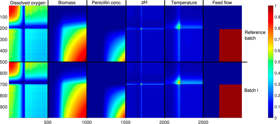
FIGURE 3. Cross-auto-correlation matrix for two batches of the Pensim process.

FIGURE 4

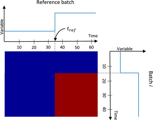
FIGURE 4. Cross-correlation matrix for a step change.

Once the informative columns from $\mathit{\Sigma }$ are identified all other columns turn redundant and can be discarded. t-SNE method is then applied to ${\mathit{\Sigma }}_{[\zeta \times \left(R+1\right)]}^{\prime }$, which is the reduced version of $\mathit{\Sigma }$. In ${\mathit{\Sigma }}^{\prime }$ one additional column has been added to account for the time progression of each batch. This input accounts for the sequential nature of the process, and it is scaled to the range of the other variables, i.e., $\left[\mathrm{0,1}\right]$. The time progression is computed as the time of every data point divided by the total duration of each batch. The conditions for the application of t-SNE are the standard Euclidean distance and the approximation based on the Barnes-Hut method. The exact t-SNE optimization method was not considered due to the high number of elements in the data set, which is the same number of rows in ${\mathit{\Sigma }}^{\prime }$, i.e., ζ. The perplexity parameter, which as explained before is a measure for the overall expected number of neighbors, can be interpreted as the minimum number of time instances that are expected to be part of a single phase, multiplied by the number of batches in the training data set, i.e., $l_{phase}\times n$. The reason is that all time instances for all batches belonging to the same process phase are expected to be neighbors in the embedded low dimensional space. The application of t-SNE to the data in the R-dimensional space results on embedding the data into a two dimensional space. Figure 5 shows the t-SNE reduced space on which the data from ${\mathit{\Sigma }}^{\prime }$ has been embedded. This visualization already demonstrates the reason for using t-SNE as technique for manifold learning and dimensionality reduction with the aim of phase identification. Since t-SNE finds the location for every data point in the reduced space as the result of an equilibrium of repulsion and attraction forces between points, the embedded space will favor the formation of clusters where similar points come together. In this application it means that points that belong to the same process phase will be separated from those that belong to other phases.

FIGURE 5

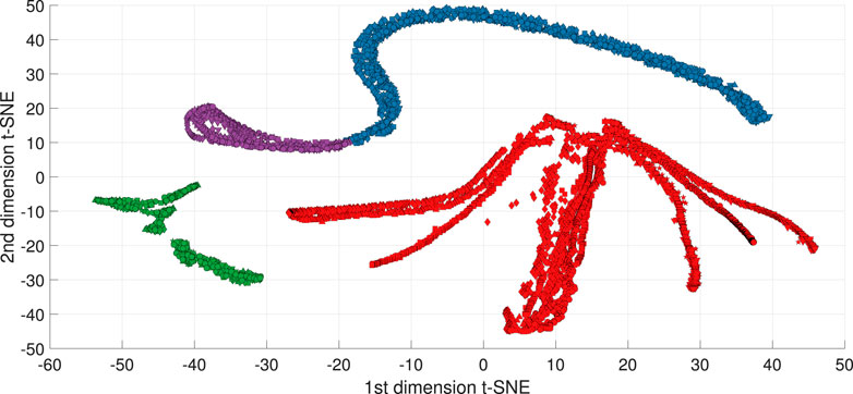
FIGURE 5. t-SNE embedded space for Pensim process.

The final step of this stage is to assign a class to the clusters formed in the reduced space obtained via t-SNE. Due to the ability of t-SNE to form separate clusters for groups of neighboring data points, this task is highly successful and can be performed with standard methods as k-means with a test criteria such as the Davies-Bouldin index (Thakare and Bagal, 2015) to automatically determine the number of clusters present in the t-SNE space. Density based spatial clustering methods such as DBSCAN (Ester et al., 1996) are preferred when clusters with arbitrary forms are present in the embedded space. The labeling of the classes is performed based on the identified clusters but following two logic rules. First, a cluster takes a label for a process phase if this contains data points from every batch in the training data set. This means that only common process conditions observed in all batches are identified as valid process phases. In case other clusters are formed in the embedded space which do not have data points from every batch in the data set, they are associated with out of trend conditions. Secondly, the labels are assigned as a numerical discrete sequence based on the know progression of the process. It must be clarified that due to the nature of the manifold learning applied via t-SNE, the location of the clusters in the reduced space do not reflects the sequential order of the process phases. The colors of the embedded points in Figure 5 are assigned based on the clusters identified using DBSCAN.

As shown in Figure 3 the completion of this stage results on three elements that are relevant for the next stage of the algorithm, i.e., 1) the time points on the variables of the reference batch which were found to be sufficient to construct the cross‐correlation matrix ${\mathit{\Sigma }}^{\prime }$, 2) the embedded map obtained from the application of t-SNE and 3) the number of sequential phases identified as clusters in the embedded map and the corresponding labeled data.

Offline Training

As shown in Figure 1, the model training stage consists of two supervised learning steps based on SVMs. First, the regression model is trained to reproduce the manifold learning obtained from t-SNE. This step is required because t-SNE is a non-parametric method that do not to allow mapping new data to an already learned embedded space. Thus, one needs to rely in other methods to apply this transformation to the new data. Secondly, classification is performed based on independent one-vs-all SVM models trained for the binary classification of every identified process phase. This means that every model evaluates the membership of the data to the phase for which the model was trained. Figure 6 depicts the structure of the machine learning method described in this paper. This figure represents the transformations applied by the described methods and their use to move from the original cross-correlation space to the phase classification in the 2-dimensional embedded space.

FIGURE 6

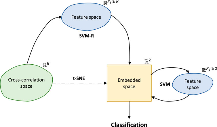
FIGURE 6. Manifold learning and clustering for phase classification.

The training and cross-validation of the SVM for regression is performed using ${\mathit{\Sigma }}^{\prime }$ as input and the corresponding coordinates in the t-SNE embedded space as responses. As opposed to the version of ${\mathit{\Sigma }}^{\prime }$ used for the original phase identification, the extra column used to impose the sequential character of the process is in this case the count of completed phases at every data point. This means that the SVM models take the knowledge of the number of phases that have already been completed at a given time in the process as an input. For the online implementation, this variable is updated every time a new process phase starts. 5 fold cross-validation is used to train the regression model preventing overfitting. Figure 7 shows the results obtained on the manifold learning using the SVM regression models. The comparison of these results with Figure 5 shows that the trained SVM models for regression approximate the embedding and clustering obtained from t-SNE. The results on the three cases evaluated show that this approximation is enough for the current application.

FIGURE 7

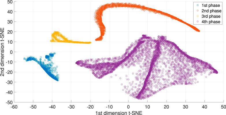
FIGURE 7. Manifold learning via SVM-regression for the Pensim process.

The output from the SVM regression model is used to train the sequential SVM classification models. Additional dummy data is generated to improve the classification performance of every individual SVM. This dummy data is generated using the same data points from ${\mathit{\Sigma }}^{\prime }$ but with a wrong assignment of the completed phase count. This dummy data allows to train the SVM model to distinguish wrongly labeled data from data with the correct membership assignment. The SVM regression mapping model is used to embed the dummy data on the 2-dimensional space. The resulting embedding for the dummy data does not follow the transformation obtained from the application of t-SNE because this data was not present on the initial dimensionality reduction. Nevertheless, this serves the purpose of discriminating correctly labeled data from that with a wrong phase label. Additionally, this allows a better definition of the boundaries for classification around the cluster in the embedded space. Figure 8 shows the boundaries obtained for the clusters representing each of the identified phases in the Pensim process. These borders are drawn by evaluating a grid of discrete points of the 2-dimensional embedded space. These results demonstrate how this method can also be used for online visualization of the progress of the process through its different phases. Finally, it can also support the early identification of deviations in the process, which can be seen as data points that are embedded into out of phase regions.

FIGURE 8

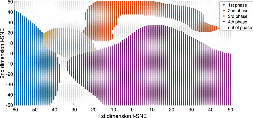
FIGURE 8. Classification boundaries for every identified phase of the Pensim process.

The final part of this stage is to determine a fixed time duration for each phase in the process. This duration will be used to align every phase in every batch. The algorithm proposed in this paper is based on the time interpolation to sub-sample the data so the final duration per phase is the same for every batch. The algorithm selects the shortest duration of every phase found in the training data as the fixed duration to which all other batches will be aligned. This means that for every phase in every batch a time compression factor $\tau \ge 1$ is determined. Thus, the time series for each variable is sub-sampled based on τ, resulting in a new data set ${\mathit{X}}_{[n\times m\times l_{min}]}$ for which all batches have the same time duration and the process phases are perfectly aligned. The parameter τ turns into an additional variable of the process which is included as an input for the data driven modeling of the process.

Online Phase Alignment

The goal of this stage is to label every new data point measured in the current batch as member of one of the already identified process phases, and then apply the time alignment factor to synchronize the progress of the current batch with respect to historical batches. Assigning the phase label to every new data point first requires computing its cross-correlation with the reference batch. This is done based only on the R identified reference time points. This results in a single row vector with R elements. This row vector is extended with the count of the already completed phases in the current batch. This serves as the input for the SVM regression models. Once the current data point is mapped to the embedded space the programmed decision logic shown in Figure 9 is applied to determine the membership of the current data point. First, the SVM model for classification of the current phase is applied, if the output label still corresponds with the current phase then the algorithm finishes and the membership is preserved. In case the output of the SVM model indicates that the current data point does not belong to the current phase then this triggers an extra verification step. The current data point is evaluated on the SVM model for the next phase. The count of already completed phases is temporary updated by one and then the input is embedded again and evaluated by the SVM model. If this results in the current data point being member of the next phase then the label is assigned and the count of completed phases is kept. Otherwise, the current data point will be treated as out-of-phase with the label of the current phase. Several successive points found to be out-of-phase could be an early indication for an unexpected deviation in the process.

FIGURE 9

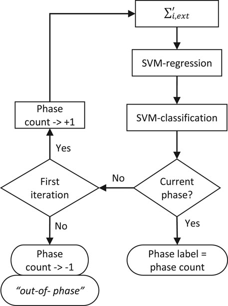
FIGURE 9. Classification decision logic for online phase alignment.

The online application of this algorithm has a low computational cost making feasible its online implementation. The complete evaluation of membership for the new data point requires in the worse case, i.e., at time points where a phase change occurs, 1) computing R product operations $O\left(R\right)$, 2) up to two applications of the SVM-regression models and 3) up to two applications of the SVM classification models, the complexity of the SVM models is linear on the number of support vectors times the number of inputs $O\left(n_{SV}R\right)$.

Since the actual sampling factor for every phase of the current batch is only known when the phase is completed, the proposed algorithm for time alignment considers applying the mean time compression factor of the phase $\left(\tilde{\tau }\right)$ while the phase is still not completed. $\tilde{\tau }$ is computed from the results obtained with the training data set. This leads to two possible extreme results: the time progression is accelerated or decelerated. The first case implies that the current phase finishes before the expected aligned time for the end of the phase. In the second case, the expected aligned time is reached and the phase is not yet completed. To solve those deviations the algorithm dynamically adapts the value of τ. In the first case τ is reduced at once to the value that guarantees the phase alignment, while in the second case τ is increased with every extra time point till the time when the phase change occurs.

Results

In this section, the final results on the application of the proposed method to the Pensim in-silico process are presented and discussed. Then the application of the method to the two industrial data sets is addressed. The industrial cases correspond to multi-phase processes which are part of the production lines of different API at commercial scale. The cases presented in this paper are a batch hydrogenation reaction and a batch centrifuge-drying process. In every case the data set available from the process consisted of several batches for which several variables were measured continuously. In every case the data was divided into training and validation sets. The computational complexity of the method proposed in this paper was evaluated based on the time required to process single data points for every case. The computational times were measured working on a laptop computer, Core i7-9750H @ 2.6 GHz and 16 MB of RAM.

Pensim Process

Figure 8 demonstrates that the implementation of the proposed algorithm on the Pensim process resulted in the identification of 4 phases for the process. Figure 10 shows the overlay plot for two of the simulated batches of the Pensim process: one from the training data set and one from the independent validation data set. Four process variables were selected to perform the phase identification and alignment following the proposed method. The trajectories of these variables display the changes occurring throughout the process. The dissolved oxygen and the pH follow smooth trajectories with information about the changes occurring during the batch stage of the Pensim process. The feed rate marks clearly the start of the fed-batch phase, and the Penicillin concentration displays the dynamic behavior during this phase. The vertical red lines in Figure 10 mark the times identified for the phase change based these variables and the proposed method. The first phase identified corresponds to the lag phase of the bacteria. During this time the bacteria adapts to the medium and not much changes are observed. The second phase corresponds with the exponential growth of the bacteria, this results in the rapid reduction of dissolved oxygen and the increase of temperature, no significant production of penicillin is observed yet. The final phase of the batch stage of this process is the extreme condition with low dissolved oxygen and low substrate concentration, increase on temperature and pH are observed and these conditions precede the start of the fed-batch operation. The final phase of the process is the fed-batch phase. In this phase the concentration of penicillin starts increasing. Figure 10 demonstrates how the proposed method is able to identify the phase changes even when they occur at very distinctive times, and with differences in the absolute values of the variables. Additionally, this case demonstrates that the method does not rely solely on variables displaying abrupt changes to identify the change on the process phase. On the contrary in this particular case the variables used for alignment, display smooth curvatures, and the manifold learning and clustering method is still able to find the partition times.

FIGURE 10

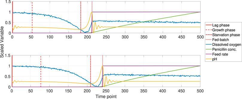
FIGURE 10. Overlay plot for two batches of Pensim with the identified phases.

The performance of the method presented in this paper was evaluated based on the results obtained for this benchmark case. Results in terms of phase identification and alignment, as well as, the impact on applications of process monitoring, i.e., fault identification and quality prediction were considered. Two reference methods reported in literature for phase identification and alignment were implemented as well to compare the performance. A set of simulated normal batches from the Pensim process were used to train the algorithms implemented for phase identification and batch alignment. The resulting pre-processed data was used to train standard PCA and PLS models. The PCA model was used for fault identification while PLS was used for regression of the output variables. It is important to mention that the focus of this paper is on the performance of the proposed algorithm for its purpose of automated phase identification and alignment, the performance for applications of process monitoring, fault identification and regression depend on the interplay with the selected modeling method.

The reference methods implemented for phase identification and alignment were the indicator variable (IV) with manual phase identification and the method proposed by Srinivasan and Qian (2007) which uses singular points for phase identification and dynamic time warping for alignment (SP-DTW). The IV method was set up to split the process in the two well known phases, i.e., batch and fed-batch, and to use the volume as indicator variable for the linear interpolation and alignment. The SP-STW method was briefly described in Section 1. The singular points were identified according with their definition over the trajectory of the dissolved oxygen. This variable was selected because it displays most of the process changes occurring during the operation, and it does not have abrupt changes due to control actions, which can be mistaken as SP. The DTW was implemented using the values [50,1,1] for the Sakoe-Chiba band constraint, and the global and local slope constraints, respectively.

The A set of four different faulty conditions were simulated for this case study. The faults are, 1) a ramp change on the feed rate, 2) a ramp change in the feed temperature, 3) the temporary reduction on the aeration flow rate, and 4) the change on the pH of the solution used to control the pH in the reactor. To evaluate the performance for fault identification, two thirds of the simulated data were used for model training, and the remaining was split into normal and faulty batches. The results obtained in terms of fault identification for the different methods and faults evaluated are reported in Table 1. These results are given in terms of the accuracy, which is the number of correctly labeled batches (normal/faulty) over the total number of tested batches, and the time delay between the know start of the fault and the detection time from the PCA monitoring strategy. The time delay was computed as the mean over the total of faulty batches. The overall results demonstrate the better performance obtained by the proposed method (tsne-SVMs) compared to the reference methods. An equally good performance is observed for the three methods with respect to the first two faults. This shows that the proposed method does not hinder the fault identification performance in cases where the deviation is unbounded and occurs directly on one of the monitored variables. In these cases, the fault can be easily picked by the monitoring strategy, and the performance seems to be independent of the phase identification and alignment method. In contrast, the fault identification performance depends more strongly on the pre-processing strategy in face of more complex faults. The third and fourth faults are examples of this. In both cases, the fault is bounded and occurs in a non-monitored variable, with an impact on the monitored trajectories. Since the implemented monitoring strategy is the same in all cases, we can conclude that the better performance for fault detection is thanks to the pre-processing method. Figure 11 shows the trajectories for two faulty batches in the case of the temporary reduction in the aeration rate. The original data for the dissolved oxygen is shown together with the data trends after alignment using SP-DTW and the proposed algorithm. Additionally, the online monitoring plot for the overall mean squared error is presented. The last plot includes the threshold for normality, based on the 95% confidence interval. Figure 11 clearly shows that the effect on the trajectory due to the DTW hinders the presence of the deviation in the faulty batches. In contrast, the proposed method does not distort the variable trajectory and therefore the deviation from the normal behavior prevails in the data after alignment. As result, the monitoring method is able of identifying on time this type of deviation. Regarding the last fault, it can be seen that the effect of the alignment technique is not as decisive as in the previous fault. However, in this case, it is still the case that a better performance is obtained when using the proposed approach. The observed improvement respect to the reference method is on both the detection time and accuracy.

TABLE 1

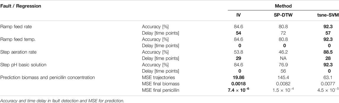
TABLE 1. Process monitoring applications on the Pensim process using different methods for phase identification and alignment.

FIGURE 11

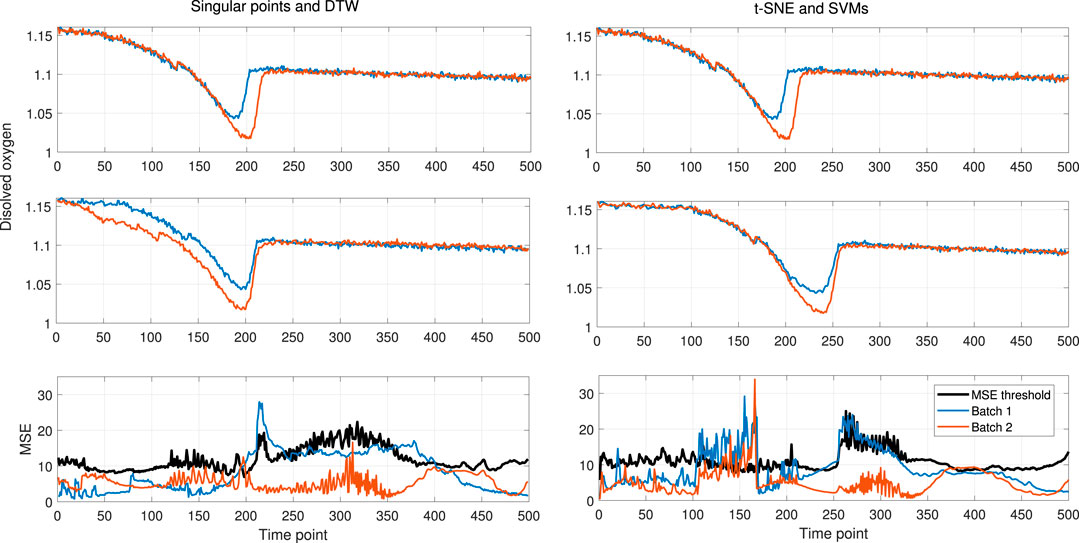
FIGURE 11. Results on the fault detection for the Pensim process. Temporary drop in the aeration rate.

Finally, an offline PLS model was trained to predict the biomass and the penicillin concentration throughout the process. The results in terms of the mean squared error (MSE) over the predicted trajectories for the two outputs, as well as the MSE on the estimation of the final concentrations, are reported in Table 1. These results show that the accuracy is higher when the proposed algorithm is used, compared to the SP-DTW method. However, the best performance is obtained using the simple IV. Figure 12 shows the trajectories for the biomass and the penicillin concentration throughout the process. The aligned data trajectories, based on the application of the two compared methods, are overlaid with the resulting prediction from the PLS model in every case. The obtained trajectories in the case of SP-DTW display variability which is not original from the process but that results from the compression/expansion applied during DTW. The added variability affects the performance of the PLS model and results on the largest error not only along the trajectory but also in the end point. In contrast, the proposed algorithm for alignment reproduces correctly the smooth trajectory of the two outputs along the different phases of the process without undesired variability being introduced into the regression model.

FIGURE 12

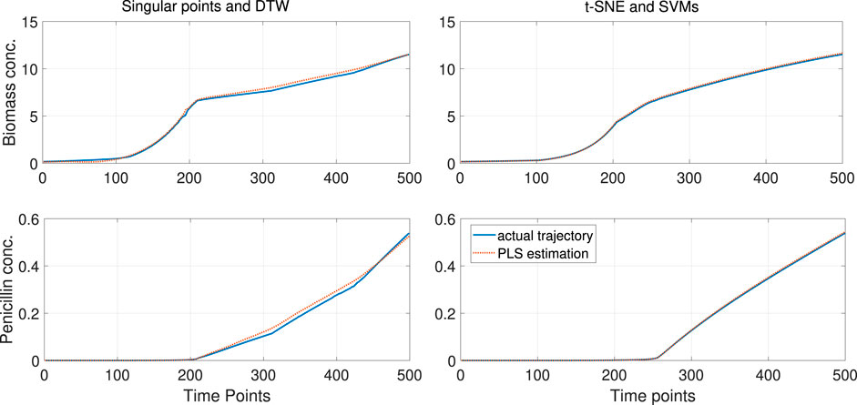
FIGURE 12. Predicted trajectories for biomass and penicillin concentration based on PLS.

Batch Hydrogenation Reaction

This case consists of a highly exothermic hydrogenation reaction that is completed as a sequence of four consecutive reaction cycles. In every cycle hydrogen is fed in the reactor to induce the reaction, then the flow is stopped to prevent the pressure to rise about safety limits in the reactor. The reactor partially cools down and a new cycle is started. Hydrogen flow, pressure in the reactor, reactor temperature and bottom temperature are the variables selected to perform phase identification. As in the Pensim case, the main driver for the selection of these variables is the information contained in their trajectories. The hydrogen flow and reactor pressure clearly display the four reaction cycles while the temperatures contribute to identifying the overall progression of the process because they increase with each new cycle. 15 batches are used for training while the obtained models for phase identification and alignment are validated on 10 independent batches.

Figure 13 shows the results obtained regarding the clusters on the embedded map (Figure 13A), the regions learned from the SVMs models for phase classification (Figure 13B), and the overlay plot of the variables used for phase identification, indicating the partition obtained by the proposed algorithm (Figure 13C). This case illustrates the application of the proposed method to a multi-phase processes that consists of repetitive cycles of similar operations. The results show that the method is not always able to discriminate the same operation being repeated several times in the process as different phases. In Figure 13A it can be seen that the embedded data points for the second and third hydrogenation cycle come very close together and the clustering method does not discriminate them as two separate clusters. However, this does not affect the online phase alignment because the partition time at the start of the third hydrogenation cycle, i.e. red dashed line in Figure 13C, is identified when the classification algorithm identifies that the second intermediate phase has ended. However, the SVM classification model for the second hydrogenation cycle should be evaluated. An alternative solution to this condition is to perform a more detailed work on clustering or tuning the perplexity of the original t-SNE so the two phases can be discriminated in separate clusters.

FIGURE 13

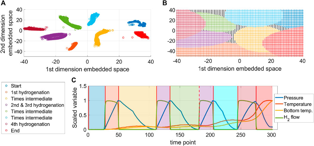
FIGURE 13. Results on the phase identification for an hydrogenation reaction.

Finally, an interesting observation of the distribution of clusters in the embedded space is the fact that the clusters for similar phases appear close to each other. In Figures 13A, B it can be seen that the clusters for the start and end of the reaction are located at the right of the embedded space, while the clusters corresponding to the hydrogenation cycles are together at the left of the space, and the intermediate phases are located in the center of the space.

Batch Centrifuge Drying

A centrifuge dryer is a unit operation that combines in a single equipment the centrifugation and drying processes for crystallized materials. The centrifugation step separates the mother liquid from the solid material and wash-out possible residual impurities. After this process phase is completed, the flow of gas starts and then the gas stream is heated to drive the evaporation of the residual solvents. The variables considered in this case for the phase identification and alignment are the temperature of the gas at the inlet, the flow of gas and the temperature inside the main chamber of the unit. From the process description, it is clear that the trajectories of the gas flow and temperature describe well the phase changes occurring in this process, in particular during the drying stage. The temperature inside the equipment contributes also to identify the changes during centrifugation because some evaporation of the solvent occurs once the centrifuge starts spinning and therefore the temperature reflects this phenomenon. 20 batches are used to train the algorithm and the results are validated in the same number of batches. Figure 14 depicts the results of the application of the proposed method to this process. Similar to the previous case, this figure shows the results obtained for the clusters in the embedded space (Figure 14A), the boundaries for phase classification based on the trained SVM models (Figure 14B), and finally an overlay of the variables to demonstrate where the phase partition times were located (Figure 14C). Compared to the previous cases, this process has the higher number of non-repetitive phases on the process. A total of six phases were identified using the proposed algorithm. These phases correspond to the known stages of the process demonstrating the validity of the results. For both cases, the hydrogenation reaction and this case, despite the large number of process phases and therefore the high number of clusters in the embedded space, the ability of t-SNE to form well defined clusters of similar points allows a robust classification of the data points. Additionally, in this case due to the larger differences between the process conditions of every phase, the regions identified for classification of every cluster are more compact, with a larger presence of the embedded space that is not associated to a particular phase allowing for a more informative classification for cases with deviations in the process.

FIGURE 14

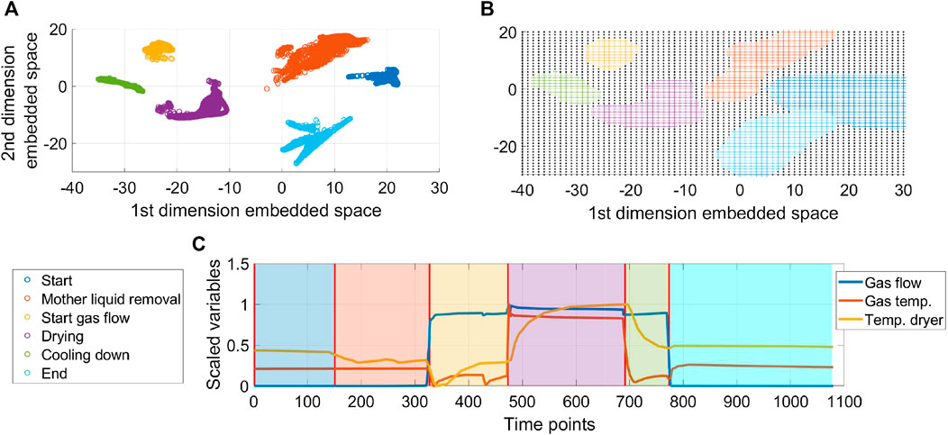
FIGURE 14. Results on the phase identification for the centrifuge drying process.

The mean time to compute the membership per data point was of around 30 $\mu s$ for the Pensim and the hydrogenation reaction cases, while for the centrifuge-drying case, it was of around 200 $\mu s$. This shows that the computational time changes from case to case, because it depends on the number of reference points R to compute the cross-correlation and the SVM regression models, but also on the number of support vectors for each SVM model. However, these results already provide a good indication of the feasibility of implementing the method proposed in this paper for online monitoring applications in industrial systems.

Conclusions

In this paper a novel machine learning method is presented to perform phase identification and alignment of data from batch processes based on manifold learning and clustering. This method exploits t-SNE to generate an embedded low dimensional map of the cross-correlation data between the training batches and a reference batch. The embedding results in a clear visualization of the phases occurring in the process because points that belong to the same phase appear as neighbors in the high dimensional cross-correlation space and therefore appear together as clusters in the low dimensional space. Since the information on the sequential character of the process is kept, different clusters are formed even for process phases that occur recursively. SVMs for regression are trained to model the embedding obtained with t-SNE and are used to apply the transformation to new batches. Based on the information learned, a set of SVM models are trained for supervised classification. These models identify the membership of the new data points to the previously identified process phases. The method presented in this paper for online phase identification and alignment can be used for the better implementation of data-driven modeling applications for batch processes. The proposed method was demonstrated on a benchmark case and two different real industrial cases. The benchmark case helps to demonstrate the method step by step and also to validate the results when compared to other existing methods. The industrial cases illustrate the method’s performance when applied to real data. Future work will focus on improving the methods to reproduce the manifold learning obtained via t-SNE.

Data Availability Statement

The data analyzed in this study is subject to the following licenses/restrictions: Ownership by Janssen Pharmaceutica. Requests to access these datasets should be directed to jan.vanimpe@kuleuven.be.

Author Contributions

Conceptualisation: CM, KP, and JVl; investigation and literature review: CM; resources: CM, KP, and JVl; writing, original draft preparation: CM; writing, review: CM, SB, KP, and JVl; visualisation: CM; supervision: SB, KP, and JVl; project administration: KP and JVl.

Conflict of Interest

Author KP is employed by Janssen Pharmaceutica. The remaining authors declare that the research was conducted in the absence of any commercial or financial relationships that could be construed as a potential conflict of interest.

Funding

This work was supported by KU Leuven Center-of-Excellence Optimization in Engineering (OPTEC) and the project G086318N of the Fund for Scientific Research Flanders (FWO). CM holds a VLAIO-Baekeland (HBC.2017.0239) grant.

References

Aizerman, M., Braverman, E., and Rozonoer, L. (1964). Theoretical foundations of the potential function method in pattern recognition learning. Autom. Rem. Contr. 25, 821–837.

Google Scholar

Beaver, S., Palazoglu, A., and Romagnoli, J. A. (2007). Cluster analysis for autocorrelated and cyclic chemical process data. Ind. Eng. Chem. Res. 46, 3610–3622. doi:10.1021/ie060544v

CrossRef Full Text | Google Scholar

Birol, G., Ündey, C., and Çinar, A. (2002). A modular simulation package for fed-batch fermentation: penicillin production. Comput. Chem. Eng. 26, 1553–1565. doi:10.1016/s0098-1354(02)00127-8

CrossRef Full Text | Google Scholar

Burges, C. (1998). A tutorial on support vector machines for pattern recognition. Data Min. Knowl. Discov. 2, 121–167. doi:10.1023/a:1009715923555

CrossRef Full Text | Google Scholar

Chan, T. F. (1987). Rank revealing QR factorizations. Lin. Algebra Appl. 88-89, 67–82. doi:10.1016/0024-3795(87)90103-0

CrossRef Full Text | Google Scholar

Debevec, V., Srčič, S., and Horvat, M. (2018). Scientific, statistical, practical, and regulatory considerations in design space development. Drug Dev. Ind. Pharm. 44, 349–364. doi:10.1080/03639045.2017.1409755

CrossRef Full Text | Google Scholar

Doan, X. T., and Srinivasan, R. (2008). Online monitoring of multi-phase batch processes using phase-based multivariate statistical process control. Comput. Chem. Eng. 32, 230–243. doi:10.1016/j.compchemeng.2007.05.010

CrossRef Full Text | Google Scholar

Ester, M., Kriegel, J., Sander, , and Xiaowei, X. (1996). “A density-based algorithm for discovering clusters in large spatial databases with noise.” in Proceedings of the second international conference on knowledge discovery in databases and data mining, Portland, OR, 226–231.

Google Scholar

Facco, P., Doplicher, F., Bezzo, F., and Barolo, M. (2009). Moving average PLS soft sensor for online product quality estimation in an industrial batch polymerization process. J. Process Control 19, 520–529. doi:10.1016/j.jprocont.2008.05.002

CrossRef Full Text | Google Scholar

García-Muñoz, S., and Mercado, J. (2013). Optimal selection of raw materials for pharmaceutical drug product design and manufacture using mixed integer nonlinear programming and multivariate latent variable regression models. Ind. Eng. Chem. Res. 52, 5934–5942. doi:10.1021/ie3031828

CrossRef Full Text | Google Scholar

Gins, G., Vanlaer, J., Van den Kerkhof, P., and Van Impe, J. F. (2014). The RAYMOND simulation package — generating RAYpresentative MONitoring Data to design advanced process monitoring and control algorithms. Comput. Chem. Eng. 69, 108–118. doi:10.1016/j.compchemeng.2014.07.010

CrossRef Full Text | Google Scholar

González-Martínez, J. M., Vitale, R., De Noord, O. E., and Ferrer, A. (2014). Effect of synchronization on bilinear batch process modeling. Ind. Eng. Chem. Res. 53, 4339–4351. doi:10.1021/ie402052v

CrossRef Full Text | Google Scholar

Guo, R., and Jin, Y. (2019). Phase identification and online monitoring for the uneven batch processes. IEEE Access 7, 81351–81363. doi:10.1109/access.2019.2919167

CrossRef Full Text | Google Scholar

Hinton, G., and Roweis, S. (2002). Stochastic neighbor embedding. Adv. Neural Inf. Process. Syst. 15, 833–840.

Google Scholar

James, M., and Russell, F. A. (1909). Functions of positive and negative type, and their connection the theory of integral equations. Phil. Trans. Roy. Soc. Lond. 209, 415–446.

Google Scholar

Kaistha, N., and Moore, C. F. (2001). Extraction of event times in batch profiles for time synchronization and quality predictions. Ind. Eng. Chem. Res. 40, 252–260. doi:10.1021/ie990937c

CrossRef Full Text | Google Scholar

Kassidas, A., Macgregor, J. F., and Taylor, P. A. (1998). Synchronization of batch trajectories using dynamic time warping. AIChE J. 44, 864–875. doi:10.1002/aic.690440412

CrossRef Full Text | Google Scholar

Kim, K., and Lee, D. (2014). Inductive manifold learning using structured support vector machine. Pattern Recogn. 47, 470–479. doi:10.1016/j.patcog.2013.07.011

CrossRef Full Text | Google Scholar

Kobak, D., and Berens, P. (2018). The art of using t-SNE for single-cell transcriptomics. Nat. Commun. 10, 5416. doi:10.1038/s41467-019-13056-x

CrossRef Full Text | Google Scholar

Liu, J., Liu, T., and Zhang, J. (2016). Window-based stepwise sequential phase partition for nonlinear batch process monitoring. Ind. Eng. Chem. Res. 55, 9229–9243. doi:10.1021/acs.iecr.6b01257

CrossRef Full Text | Google Scholar

Luo, L., Bao, S., Mao, J., and Tang, D. (2016). Phase partition and phase-based process monitoring methods for multiphase batch processes with uneven durations. Ind. Eng. Chem. Res. 55, 2035–2048. doi:10.1021/acs.iecr.5b03993

CrossRef Full Text | Google Scholar

Maurya, M. R., Rengaswamy, R., and Venkatasubramanian, V. (2007). Fault diagnosis using dynamic trend analysis: a review and recent developments. Eng. Appl. Artif. Intell. 20, 133–146. doi:10.1016/j.engappai.2006.06.020

CrossRef Full Text | Google Scholar

Mingxing, J., Fengxiang, L., and Shouping, G. (2010). “Optimal PCA-based modeling and fault diagnosis for uneven-length batch processes.” in 8th IEEE international conference on control and automation, Xiamen, China, June 9-June 11, 2010, (IEEE), 1731–1736.

Google Scholar

Ng, Y. S., and Srinivasan, R. (2009). An adjoined multi-model approach for monitoring batch and transient operations. Comput. Chem. Eng. 33, 887–902. doi:10.1016/j.compchemeng.2008.11.014

CrossRef Full Text | Google Scholar

Qiao, Z., Wang, Z., Zhang, C., Yuan, S., Zhu, Y., and Wang, J. (2012). An iterative two-step sequential phase partition (ITSPP) method for batch process modeling and online monitoring. AIChE J. 59, 215–228. doi:10.1002/aic.15205

CrossRef Full Text | Google Scholar

Spooner, M., Kold, D., and Kulahci, M. (2017). Selecting local constraint for alignment of batch process data with dynamic time warping. Chemometr. Intell. Lab. Syst. 167, 161–170. doi:10.1016/j.chemolab.2017.05.019

CrossRef Full Text | Google Scholar

Srinivasan, R., and Qian, M. (2007). Online temporal signal comparison using singular points augmented time warping. Ind. Eng. Chem. Res. 46, 4531–4548. doi:10.1021/ie060111s

CrossRef Full Text | Google Scholar

Srinivasan, R., and Qian, M. S. (2005). Off-line temporal signal comparison using singular points augmented time warping. Ind. Eng. Chem. Res. 44, 4697–4716. doi:10.1021/ie049528t

CrossRef Full Text | Google Scholar

Sun, W., Meng, Y., Palazoglu, A., Zhao, J., Zhang, H., and Zhang, J. (2011). A method for multiphase batch process monitoring based on auto phase identification. J. Process Contr. 21, 627–638. doi:10.1016/j.jprocont.2010.12.003

CrossRef Full Text | Google Scholar

Suykens, J. A. K., Van Gestel, T., and De Brabanter, J. (2002). Least Squares support vector machines (world scientific).

Google Scholar

Thakare, Y., and Bagal, S. (2015). Performance evaluation of k-means clustering algorithm with various distance metrics. Int. J. Comput. Appl. 110, 12–16. doi:10.5120/19360-0929

Google Scholar

Van der Maaten, L. (2014). Accelerating t-SNE using tree-based algorithms. J. Mach. Learn. Res. 15, 3221–3245.

CrossRef Full Text | Google Scholar

Van Der Maaten, L. (2009). Learning a parametric embedding by preserving local structure. Proc. Mach. Learn. Res. 5, 384–391.

Google Scholar

Van der Maaten, L., and Hinton, G. (2008). Visualizing data using t-SNE. J. Mach. Learn. Res. 9, 2579–2605.

Google Scholar

Vapnik, V., Golowich, S. E., and Smola, A. J. (1996). Support vector method for function approximation, regression estimation and signal processing. Adv. Neural Inf. Process. Syst. 9, 281–287.

Google Scholar

Wang, J., Qiu, K., Liu, W., Yu, T., and Zhao, L. (2018). Unsupervised-multiscale-sequential-partitioning and multiple-SVDD-model-based process-monitoring method for multiphase batch processes. Ind. Eng. Chem. Res. 57, 17437–17451. doi:10.1021/acs.iecr.8b02486

CrossRef Full Text | Google Scholar

Wang, K., Rippon, L., Chen, J., Song, Z., and Gopaluni, R. B. (2019). Data-driven dynamic modeling and online monitoring for multiphase and multimode batch processes with uneven batch durations. Ind. Eng. Chem. Res. 58, 13628–13641. doi:10.1021/acs.iecr.9b00290

CrossRef Full Text | Google Scholar

Wold, S., Kettaneh-Wold, N., MacGregor, J., and Dunn, K. (2009). Batch process modeling and MSPC. Comprehensive Chemometrics,2 163–195. doi:10.1016/b978-044452701-1.00108-3

CrossRef Full Text | Google Scholar

Yu, L. X., Amidon, G., Khan, M. A., Hoag, S. W., Polli, J., Raju, G. K., et al. (2014). Understanding pharmaceutical quality by design. AAPS J. 16, 771–783. doi:10.1208/s12248-014-9598-3

CrossRef Full Text | Google Scholar

Zhang, S., Zhao, C., and Gao, F. (2018). Two-directional concurrent strategy of mode identification and sequential phase division for multimode and multiphase batch process monitoring with uneven lengths. Chem. Eng. Sci. 178, 104–117. doi:10.1016/j.ces.2017.12.025

CrossRef Full Text | Google Scholar

Zhang, X., and Song, Q. (2015). A multi-label learning based kernel automatic recommendation method for support vector machine. PLoS ONE 10, 1–31. doi:10.1371/journal.pone.0120455

CrossRef Full Text | Google Scholar

Zhang, Z., Tavenard, R., Bailly, A., Tang, X., Tang, P., and Corpetti, T. (2017). Dynamic Time Warping under limited warping path length. Inf. Sci. 393, 91–107. doi:10.1016/j.ins.2017.02.018

CrossRef Full Text | Google Scholar

Zheng, S., and Zhao, J. (2020). A new unsupervised data mining method based on the stacked autoencoder for chemical process fault diagnosis. Comput. Chem. Eng. 135, 106755. doi:10.1016/j.compchemeng.2020.106755

CrossRef Full Text | Google Scholar

Zhu, W., Webb, Z. T., Mao, K., and Romagnoli, J. (2019). A deep learning approach for process data visualization using t-distributed stochastic neighbor embedding. Ind. Eng. Chem. Res. 58, 9564–9575. doi:10.1021/acs.iecr.9b00975

CrossRef Full Text | Google Scholar

Zhu, Z., Song, Z., and Palazoglu, A. (2011). Transition process modeling and monitoring based on dynamic ensemble clustering and multiclass support vector data description. Ind. Eng. Chem. Res. 50, 13969–13983. doi:10.1021/ie201792r

CrossRef Full Text | Google Scholar