Costs vs. Flexibility of Process Heat Recovery Solutions Considering Short-Term Process Variability and Uncertain Long-Term Development

To significantly decrease fossil carbon emissions from oil refineries, a combination of climate mitigation options will be necessary, with potential options including energy efficiency, carbon capture and storage/utilization, biomass integration and electrification. Since existing refinery processes as well as many of the potential new processes are characterized by large heating demands, but also offer large opportunities for process excess heat recovery, heat integration plays a major role for energy efficient refinery operation after the implementation of such measures. Consequently, the process heat recovery systems should not only be able to handle current operating conditions, but also allow for flexibility towards possible future developments. Evaluation of the flexibility of process heat recovery measures with both these perspectives enables a more accurate screening and selection of alternative process design options. This paper proposes a new approach for assessing the trade-off between total annual cost and potential operating flexibility for the heat exchanger network in short-as well as in long-term perspectives. The flexibility assessment is based on the evaluation of a flexibility ratio (similar to the conventional flexibility index) to determine the range in which operating conditions may vary while at the same time achieving feasible operation. The method is further based on identification of critical operating points to achieve pre-defined flexibility targets. This is followed by optimization of design properties (i.e., heat exchanger areas) such that feasible operation is ensured in the critical operating points and costs are minimized for representative operating conditions. The procedure is repeated for a range of different flexibility targets, resulting in a curve that shows the costs as a function of desired flexibility ratio. The approach is illustrated by an example representing a heat exchanger network retrofit at a large oil refinery. Finally, the paper illustrates a way to evaluate the cost penalty if the retrofit is optimized for one operating point but then operated under changed conditions. Consequently, the presented approach provides knowledge about cost and flexibility towards short-term variations considering also changes in operating conditions due to long-term development.

Introduction

To reach international climate targets, it is essential to significantly decrease fossil carbon emissions from the transportation sector, which will reduce the demand for traditional products from the oil refining industry, and increase the demand for fuels with low carbon footprint over the entire value chain. The oil refineries are consequently required to make substantial changes in their businesses and operations. As presented in a recent roadmap by FuelsEurope (2018), a division of the European Petroleum Refiners Association, climate mitigation options for oil refineries include energy efficiency measures (European Commission 2018), carbon capture for either long-term storage (CCS) (Andersson et al., 2016) or upgrading to enhance fuel production (carbon capture and utilization, CCU) (Fernandez-Dacosta et al., 2018), electrification (especially for hydrogen production) (Wiertzema et al., 2020), and introduction of biobased feedstock (Jafri et al., 2019). Pre-processed biobased feedstock can be integrated at different stages of existing refinery processes (van Dyk et al., 2019). Examples of pre-processing options include pyrolysis (Arbogast et al., 2012; Sharifzadeh et al., 2019), gasification (Arellano-Garcia et al., 2017) and lignin depolymerization (Jafri et al., 2019a). An efficient decarbonization strategy will most probably build upon a combination of several decarbonization options. Because of the complexity and interconnections between refinery units, carbon mitigation options will affect each other, and it is of importance to take possible future strategies into account when implementing short-term measures (Berghout et al., 2019).

One important aspect to consider when assessing the potential performance of new decarbonization processes for oil refineries at the conceptual design stage is how they can be integrated within the refinery site to ensure efficient recovery of process excess heat for a range of possible operating conditions. Many refinery process units require large quantities of heat, which makes heat integration a central option to increase energy efficiency. The use of excess heat could also be important to improve the economic and climate footprint feasibility of new processes such as the solvent regeneration of carbon capture units by avoiding the addition of new heat production capacity (Andersson et al., 2014; Biermann et al., 2021). It is common that several heat exchanger network (HEN) designs can be identified that achieve approximately the same energy saving at similar costs. However, such HEN designs can vary significantly regarding network complexity, as well as need for utility heaters and coolers for target temperature control, etc. Factors that have been shown to be important are placement of new heat exchangers (HXs), network complexity, spatial limitations and utility heaters and coolers for target temperature control (Marton et al., 2020). Therefore, it is necessary to consider technical, practical and operational factors together with capital and operational costs when evaluating alternative HEN retrofits. Consequently, an efficient use of heat and a well-designed HEN is central to achieve an energy efficient and profitable process with low carbon footprint. There are a number of well-developed methods for efficient heat integration for both retrofitting and greenfield studies, including methods based on graphical analysis (pinch analysis) and mathematical programming. For full reviews of HEN retrofit methodologies and research, see Wang et al. (2021), Sreepathi and Rangaiah (2014) and Smith et al. (2010).

Increasing heat recovery within an existing chemical process often leads to more interconnections within the process, which can potentially lead to issues related to process operability. To avoid extremely costly process interruption or safety problems, it is crucial to consider operability issues when investigating internal heat recovery measures for a chemical process. This is supported by results from Fleiter et al. (2012), who showed that candidate energy efficiency measures that are close to core production processes and that can potentially affect process operability often have a lower adoption rate.

Several studies have investigated how targets and retrofit designs for heat integration are affected by various constraints and costs related to practical limitations. An overview was presented by Chew et al. (2013) who discussed implementation issues for heat integration projects, and note design issues such as plant layout and pressure drop considerations. Such issues have received specific consideration in several studies by other authors. For example, Hiete et al. (2012) extended the pinch analysis for total sites by accounting for piping distances and additional costs for utility backup systems. Also based on insights from total site targeting, Hackl and Harvey (2015) derived practical solutions for heat integration between plants owned by different companies, and proposed a roadmap for investments to enable successively more complex business case solutions. Bütün et al. (2019) instead included costs of piping, pressure drops and heat losses in a mixed integer linear programming framework for optimization of heat integration between plants. Another recent example of layout and pressure drop consideration in heat integration is the work by Jegla and Freisleben (2020) who investigated energy retrofits considering spatial restrictions for heat exchangers and pressure drops. In addition to the aforementioned studies, several methods have been proposed to consider and evaluate the effect of restrictions on heat exchange between process units on energy targets for overall sites (see e.g., Svensson et al., 2020 for a recent example). A comprehensive mathematical formulation for such problems considering integration between plants, within separate plants and at separate process units as well as potential heat exchange restrictions was also recently proposed Kantor et al. (2020).

In addition to design considerations, the review of implementation issues for heat integration measures by Chew et al. (2013) also emphasizes several aspects of operability. Examples of studies on operability related to heat integration include the work by Setiawan and Bao (2011) who investigated how unit interactions created by, for example, heat integration, affected the plantwide operability in terms of stability and dynamic performance, and the work by Abu Bakar et al. (2016), who illustrated possible trade-offs between operability and minimum temperature difference for HENs.

Marton et al. (2020) studied different aspects of operability as well as practical implementation issues related to HEN retrofits at an oil refinery. The study, which was based on interviews with refinery engineers, found that factors such as spatial limitations, pressure drops and non-energy benefits significantly influence the potential for a positive implementation decision for the heat recovery measures and that it is important to consider those factors early in the design of heat recovery measures. One of the aspects that was covered in the interviews was how process flexibility was expected to be affected by the retrofits, but no clear results were obtained regarding the effect, and how this would influence a decision to invest in the measure. Potential issues were discussed but it was also concluded that a more in-depth study would be needed to thoroughly investigate the potential impacts of heat recovery measures on process flexibility. This is now the focus of the present paper.

The flexibility of a HEN can be defined as its ability to handle variations. Short-term flexibility is often required to maintain feasible operation on a daily operating basis. However, it is undoubtably advantageous if new process heat recovery solutions can also be evaluated with respect to expected long-term development. Such expected long-term changes differ fundamentally from short-term variations. For example, the refinery heat recovery systems should be sufficiently flexible to allow for efficient operation also when future development of refinery technologies and processes leads to significant changes in operating conditions. Such long-term developments could include significant changes in process throughput or compositions of process flows, changes in steam balances or new input or required targets for temperatures caused by changes in reactions or separation processes. Consequently, it is important to also address this demand for long-term flexibility when designing retrofit projects which aim for energy savings by increased heat recovery. A systematic evaluation of the flexibility of process heat recovery measures enables a more accurate screening and selection of alternative process design options. This is of special importance if there are alternative proposals with comparable energy savings potential and capital costs for nominal operating conditions, but with significantly differing performance when operating conditions deviate from nominal design conditions. Additionally, evaluating the economic impact of flexibility provides guidance for when flexibility should be considered in the decision-making process when implementing heat recovery measures.

The problem of finding the optimal design configuration to ensure minimal cost (investment and operating) while allowing for variations in operation conditions has been studied extensively in literature since the early works of Marselle et al. (1982) and Grossmann et al. (1983). An overview of methodologies for synthesis of flexible HENs was recently presented in a review paper by Kang and Liu (2019). Some recent developments in this area include flexibility for site wide integration (Kachacha et al., 2018), a robustness indicator based on enhanced data collection (Payet et al., 2018), use of Monte Carlo simulation to analyze flexibility and controllability of HEN retrofit designs (Lal et al., 2019), a new HEN synthesis methodology that considers flexibility with respect to both process fluctuations and gradual build-up of fouling (Liu et al., 2019), break-even analysis to find the probability of fluctuations that make over-design for flexibility beneficial (Hafizan et al., 2020), flexibility assessment accounting for both measurable and unmeasurable parameters (Ochoa and Grossmann 2020), and a new optimization strategy based on binary particle swarm optimization and an evolutionary algorithm for solving the problem of synthesis of flexible HENs (Wang et al., 2021). However, to the authors’ knowledge no systematic approach has been published to guide the analysis of the trade-offs between investment cost and benefits associated with flexibility for both short-term flexibility and long-term development.

This paper aims to present a systematic approach for assessing the trade-offs between costs and benefits associated with flexibility of heat recovery measures. The approach considers operational variations around a nominal operating point in a short -term perspective as well as potential long-term changes or developments of the nominal operating point. Additionally, the proposed approach provides cost estimations for designs optimized for the investigated range of variations. Short-term flexibility is assessed in an approach based on the flexibility index, with costs estimated for critical and representative operating points. Long-term flexibility is handled by evaluating the sensitivity of the solutions to long-term changes as well as by optimizing the design for the different operating points over the lifetime of the investments. An illustrative example is used to demonstrate the developed approach.

Variations and Long-Term Development

A refinery needs to be flexible enough to adjust to variations of different kinds. The process and thereby the HENs used for process heat recovery are affected by ambient conditions, feedstock variations and varying product demands. These can be classified as short-term variations, typically ranging from hourly or daily to seasonal scale. The effect of cooling fans is, for example, highly dependent on the temperature of the ambient air, which varies over the year, which can lead to lower cooling capacity in the HEN. Depending on crude oil prices and carbon taxes, it is profitable to process different compositions of crude feedstocks. The most cost-effective product mix depends on market scenarios and crude mix. Variations in the crude oil and product mix affect the compositions of process flows in the different refinery units, which inherently affect the temperature requirements and fractions wanted in separation columns as well as the demands and targets for steam and heat recovery systems. Another factor that varies in refinery production is catalyst degradation, which creates a demand for higher temperatures in reactors during later stages of the catalyst degeneration cycle.

Long-term developments due to the integration of new processes or larger shifts in production are likely to lead to a permanent change of typical, average operating conditions. However, short-term variations affecting the process might also change. For example, it is possible that the day-to-day production will vary more (or less) in future refinery operations. Major changes required to meet stringent climate mitigation targets will significantly affect refinery production and thereby create new operating points. New operating conditions will put other demands on the existing heat recovery systems and are likely to change the overall energy balances for the refinery (van Dyk et al., 2019). For example, introduction of partially pre-processed biomass feedstock for final processing in refinery units could affect throughputs of process units relative to each other, and thereby change the opportunities for heat recovery between such units. Carbon capture, as another example, requires substantial amount of heat to drive the capture process, which may limit the excess heat available for energy efficiency measures from both hot process streams and from low pressure steam (Andersson et al., 2014). Additionally, electrification of different processes will consequently affect the energy system and available heat in the refinery (Wiertzema et al., 2020).

Methodology

The flexibility assessment is based on the evaluation of the flexibility index (Swaney and Grossmann 1985) to determine the range in which operating conditions may vary while still achieving feasible operation. In this context, feasibility is assumed to be achieved when predefined target values, e.g., target temperatures of streams, can be reached for all possible operating points within the identified range of variation. Furthermore, the minimum total annualized costs are determined for a heat recovery measure under different assumptions about the operational variations to which it will be exposed, i.e., for different flexibility requirements.

Theoretical Background

The common aim of available methodologies for flexibility analysis is to indicate the maximum variation range in which inlet conditions may vary while at the same time achieving feasible operation. This maximum variation range can be interpreted in different ways and a common interpretation is to set the maximum feasible variation range in relation to an expected variation range which is defined by lower and upper bound values. This interpretation is the basic concept of the flexibility index which was introduced by Swaney and Grossmann (1985). Such a variation range can be imagined as a hyperrectangle (multi-dimensional rectangle, e.g., cuboid for three dimensions) and the maximum feasible variation range is consequently the largest scaled hyperrectangle which fits into the feasible region. This is illustrated in Figure 1.

FIGURE 1

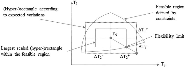
FIGURE 1. Illustration of the flexibility index as a flexibility analysis methodology to identify the largest feasible variation range of a design/process defined by mathematical constraints.

In Figure 1, the point marked as “flexibility limit” limits the size for the largest rectangle which fits into the feasible region. If this limitation is caused by the available (or planned) equipment size, the equipment size can be modified to adapt to the required level of flexibility. This is illustrated in Figure 2, in which it is shown how the feasible region is altered when the equipment size is changed, as well as how the equipment size influences the feasible variation range. It should be noted that there is an upper bound for the adaptation of the equipment size which depends on the fundamental structure of the design, i.e., at this upper bound the flexibility is not limited by the available equipment size. This upper bound can be referred to as the structural flexibility bound [see e.g., Li et al. (2014) and further information and examples can be found in Langner et al. (2020)].

FIGURE 2

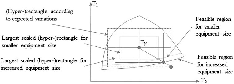
FIGURE 2. Illustration alteration of feasible region when the equipment size is changed, and its influence on the feasible variation range.

Trade-Offs Between Costs and Flexibility

From Figure 2, one can identify the (intuitive) correlation between equipment size and benefits associated with flexibility, i.e., larger equipment size (in combination with operational controls such as heat exchanger bypasses to allow for partial load) allows for maintaining feasible operating when larger variations occur. Consequently, a trade-off can be recognized between investment cost/equipment size on the one side and benefits associated with flexibility on the other side. An interesting question that arises is to define the type of function that best describes the correlation between costs and the flexibility to handle variations, i.e., does the relationship follow a linear, polynomial, exponential, etc. trend? Furthermore, if such a trade-off analysis reveals an over-proportional increase in necessary investment cost when the variation range increases, measures to prevent or limit the variations range, which are usually more costly, i.e., to handle variations up-stream of the process in question, may become more beneficial. However, to reveal such insights, a systematic approach is necessary to analyze the trade-off between the costs and benefits associated with flexibility.

For such an analysis, the term expected variation range may be misleading or even problematic, if the expected variation range is itself uncertain, e.g., if variations can be handled up-stream of the process in question (more efficiently?) or if the available historical data is incomplete, the expected variation range is rather a theoretical concept in order to perform flexibility analysis. Additionally, one could interpret the expected disturbance range as a target value for the flexibility, i.e., if the maximum feasible disturbance range matches the expected disturbance range the flexibility demand is satisfied. On the other hand, Figures 1, 2 show that the expected variation range has a significant influence on the geometric form of the maximum feasible variation range (largest scaled hyperrectangle within feasible region) since the expected variation range defines the aspect ratio of the identified maximum variation range. Therefore, we suggest defining a nominal variation range which defines the aspect ratio of the feasible variation range (when performing flexibility analysis) but which does not (necessarily) define a target value for the flexibility demand. The nominal variation is thus simply used as a reference to which the feasible variations are related to allow for expressing a ratio similar to the flexibility index. Following the definition of the flexibility index, we define a flexibility ratio as the ratio between the feasible variation range and the nominal variation range.

$flexibility\hspace{0.5em}ratio= \frac{feasible\hspace{0.5em}variation}{nominal\hspace{0.5em}variation}(1)$

Even if the flexibility ratio cannot be interpreted in the same way as the flexibility index, it should be noted that it can be calculated the same way as the flexibility index, e.g., utilizing the active set approach which was introduced by Grossmann and Floudas (1987).

In order to evaluate the trade-off between costs and benefits associated with flexibility we therefore suggest estimating the costs as a function of the flexibility ratio:

$Costs=f\left(flexibility\hspace{0.5em}ratio\right)(2)$

Such a function cannot be formulated explicitly but needs to be approximated using nodes, i.e., determine the costs for a discrete number of pre-defined flexibility ratios. To establish the costs associated with new process heat recovery solutions, e.g., heat exchanger network retrofit, for a specific flexibility ratio (i.e., one node of the desired function) both investment and operating cost need to be considered. The Total Annualized Cost (TAC) combines annualized investment cost [which depends on the expected (or remaining) lifetime of the investment] with annual operating cost in a single metric. For a given structural design proposal, the optimal value for TAC can be identified by solving optimization problem P1 (see Langner et al. (2020).

$\begin{array}{l}\underset{\text{x},\text{z},\text{d}}{\min }\text{TAC}={\text{c}}_{\text{operating}}+{\text{c}}_{\text{investment}}\text{*CRF}\hfill \\ \text{s}.\text{t}.\hfill \\ {\text{h}}_{\mathrm{i}}\left(\text{x},\text{z},\text{d},{\text{θ}}_{\text{op}}\right)=0;\hspace{0.5em}\text{i}\in \text{I}\hfill \\ {\text{g}}_{\mathrm{j}}\left(\text{x},\text{z},\text{d},{\text{θ}}_{\text{op}}\right)\le 0;\hspace{0.5em}\text{j}\in \text{J}\hfill \\ {\text{g}}_{\mathrm{d}}\left(\text{x},\text{z},{\text{θ}}_{\text{op}}\right)-\text{d}\le 0;\hspace{0.5em}\text{d}\in \text{DV}\hfill \\ \text{d}\ge 0\hfill \\ \text{x},\text{z},\text{d},{\text{θ}}_{\text{op}}\in \text{R},\hspace{0.5em}{\theta }_{\text{L}}\le {\text{θ}}_{\text{op}}\le {\theta }_{\text{U}}\hfill \end{array}$P1

In P1, TAC consists of the annual operating cost c_operating in €/year (utility cost) and the investment cost c_investment in €, which is annualized with the given capital recovery factor CRF. The performance data (e.g., heat exchanger duties) required to estimate the operating cost are calculated using the set of equality constraints h_i with i∈I (heat and mass balances) and the set of inequality constraints g_j with j∈J (temperature and other operational restrictions). The investment cost depends on the set of the non-negative design variables d (e.g., heat exchanger areas) with d∈DV, which are calculated using the corresponding design constraints g_d.

In h_i, g_j, and g_d, x is the vector of the state variables, and z corresponds to the control variables (e.g., bypass ratios). Furthermore, the varying inlet conditions are depicted by θ which are limited by a lower bound (θ_L) and an upper bound (θ_U). The lower and upper bound for the varying inlet conditions are defined by the fixed flexibility ratio (i.e., percentage of the nominal variation range). Since the interval between θ_L and θ_U includes infinitely many values, a discrete set of operating points (op) needs to be defined to solve P1. This set of operating points must include the critical operating points to ensure that the obtained solution for the design variables (i.e., equipment size) matches the demanded flexibility ratio. Such critical operating points can be identified prior to solving problem P1 using the framework presented by Langner et al. (2020) which builds upon methodologies introduced by Pintaric and Kravanja (2008). In addition to the critical operating points, further operating points need to be included whose choice depends on the chosen way to calculate the annual operating cost (see above). Finally, to determine the optimal value for TAC (for the respective operating points), the degrees of freedom of the optimization problem are the non-negative design variables d with d∈DV and the control variables (of the HEN) z.

Proposed Procedure to Approximate Total Annualized Cost as a Function of the Flexibility Ratio

In the following, the approach outlined above to approximate the function TAC(flexibility ratio) is summarized. Examples can be found in Results. For simplicity, TAC was calculated for a single nominal operating point which does not change for different target values of the flexibility ratio.

1. For retrofits: determine existing design specifications (e.g., HX areas, tank capacities, etc.)

2. Identify varying inlet conditions and define nominal variation ranges

3. For retrofits: determine flexibility ratio of existing and/or conceptual retrofit design (for comparative reasons)

4. Determine minimum TAC by solving P1 without consideration of critical operating points

➢ Flexibility ratio of obtained design represents the lower bound for the flexibility ratio

5. Define target values for the flexibility ratio (>lower bound values obtained in Step 4) and determine corresponding critical operating points utilizing the framework of Langner et al. (2020).

6. Determine minimum TAC by solving P1 for the different target values of the flexibility ratio including the corresponding set of critical operating points identified in Step 5.

7. Approximate TAC (flexibility ratio) based on the nodes obtained in Step 6, e.g., by interpolation.

It should be highlighted that the solution of P1 for each flexibility ratio does not only include the TAC to ensure the specified flexibility target but also the necessary equipment size of the process units. Consequently, each node obtained can be interpreted as a (stand-alone) design with specified equipment size.

Additionally, it should be highlighted that the calculations in the above-outlined procedure (Steps 4, 5 and 6) can be automated using available tools for automated heat exchanger network modelling [e.g., Langner et al. (2021)], the calculation of the flexibility ratio using tools for the automatic calculation of the flexibility index mentioned [e.g., in Ochoa and Grossmann (2020)], and for the determination of the critical operating points [e.g., Langner et al. (2020)].

Analyzing Flexibility with Respect to Expected Long-Term Development

The approach described above is well-suited to analyze the trade-offs between costs and benefits associated with the flexibility to handle variations around a nominal operating point. While short-term variations usually refer to disturbances from nominal operating conditions which require recursive actions in order to minimize the impact of the variations on the process output, long-term changes commonly result of planned modifications (e.g., in the design or operation of the process). In this paper, long-term changes are modeled as a permanent alteration of the nominal operating point to a new nominal operating point while nominal short-term variations around the operating point are (not necessarily) affected by this alteration. This is visualized in Figure 3.

FIGURE 3

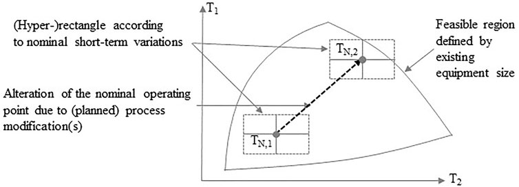
FIGURE 3. Long-term changes modeled as a permanent alteration of the current nominal operating point (nominal point 1) to a new nominal operating point (nominal point 2) while nominal short-term variations around the operating point(s) are not affected by this alteration.

To understand the effects on costs and flexibility of long-term developments involving a change of nominal operating point, it is desirable to perform two different types of evaluations:

1. Sensitivity analysis of the solutions obtained for nominal point 1, to obtain knowledge about how the TAC and flexibility for these solutions are influenced by a change of other operating conditions

2. Estimation of a new TAC (flexibility ratio) function, which is optimized for the expected operating conditions over the lifetime of the investments

The strategies required to perform the above evaluations are outlined below.

Sensitivity Toward Long-Term Development

The goal of this kind of evaluation is to obtain knowledge regarding how the costs and flexibility estimated for the current operating point (i.e., nominal point 1) would be affected by long-term changes (i.e., permanent alteration of the nominal operating point). To do this, we suggest solving a simplified version of P1 for each design representing a node in the original trade-off function [TAC (flexibility ratio)] to obtain the TAC for this design/node when operation is shifted to nominal point 2. A simplified version of P1 is sufficient because for each node/stand-alone design, the design variables d with d∈DV are fixed. Consequently, the investment cost is fixed, and the solution of this simplified optimization problem is the configuration of control variables z which yield the minimum annual operating cost c_operating in €/year (utility cost) for the respective design at nominal point 2.

Furthermore, one needs to evaluate the flexibility ratio of each design/node around nominal point 2 by solving the flexibility index problem—utilizing e.g., the active set approach by Grossmann and Floudas (1987)—for an updated or the previously defined nominal variation range. For the case that the modifications causing the switch to nominal point 2 influence the short-term variations in any way, this must be reflected in an updated nominal variation range.

By following the above outlined strategy, the influence of the new operating conditions on costs and flexibility of the solutions identified for nominal point 1 can be determined.

Optimization for All Operating Points Expected Over the Project Lifetime

The goal of this approach would be to estimate the optimal trade-offs between costs and flexibility, while considering that the process might operate under different operating conditions over the lifetime of the investment. However, this requires assumptions regarding the actual timepoint of the process modification (alteration of the nominal point)—in order to know how the operating costs of different operating periods should be weighted against each other. Suggestions for how to handle this are presented in Economic Calculations. Additionally, it was necessary to develop a concept to allow for incorporating the alteration of the nominal operating point when evaluating flexibility with respect to short-term variations. This concept is introduced in Section.

Overall Flexibility Ratio

When a process operates at multiple nominal operating points, e.g., due to a switch of operation, and short-term variations such as disturbances occur around each nominal operating point, we suggest to determine the flexibility ratio for each nominal operating point (considering the corresponding nominal variation range) and define the lowest value as the overall flexibility ratio.

The overall flexibility ratio can be explained using Figure 3. Figure 3 shows a case where operation at the new operating point (nominal point 2) is much more restricted with respect to the magnitude of feasible short-term variations compared to the operation at the current operating point (nominal point 1). Consequently, if operation at both nominal points is expected, the overall flexibility (with respect to short-term variations) is limited by the feasible variations range around nominal point 2, i.e., the flexibility ratio at nominal point 2 is smaller compared to the flexibility ratio at nominal point 1.

A strategy is also needed to ensure that a pre-defined target value for the overall flexibility ratio can be guaranteed by a solution of P1 for any combination of expected nominal operating points. The premise for such a strategy is that all nominal operating points and the corresponding nominal short-term variations around these operating points are known a-priori. In such a case, we suggest to determine, for each expected nominal operating point, the corresponding set of critical operating points [following Langner et al. (2020)] and eventually include all identified critical operating points when solving P1 to obtain the TAC for the respective overall flexibility ratio. This way, it is guaranteed that the defined target value for the overall flexibility ratio is achieved for operation at each nominal operating point while for some operating points the flexibility may be larger, i.e., the defined overall flexibility ratio target can be imagined as the minimum flexibility requirement for operation at the current and any expected nominal operating point.

Economic Calculations

In order to calculate the TAC utilizing P1, it is necessary to define a (nominal) operating point (or several representative points, see explanation of P1) for calculating the annual operating cost. When operating at two (or more) nominal operating points during the expected/remaining lifetime of the process, it is therefore necessary to define the exact timepoint(s) of the alteration(s) in order to define weight factor(s) to fairly distribute the operating cost over the expected lifetime. This is problematic if the exact timepoint of an alteration is unknown. To avoid an explicit assumption of the timepoint of the alteration from nominal point 1 to a new nominal point 2, we suggest approximating trade-off functions representing the two extreme cases with respect to the timepoint of the process change:

a) The nominal point remains at nominal point 1 through the entire economic lifetime The corresponding function TAC_a (overall flexibility ratio) is then defined as the minimum total annualized cost such that the process achieves the required flexibility ratio at both nominal point 1 and 2, but during the entire expected lifetime of the process the process is only operated at nominal point 1 (e.g., process modifications are not carried out or have no effect on the nominal operating point).

b) The nominal point is changed to nominal point 2 immediately after start of operation The corresponding function TAC_b (overall flexibility ratio) is then defined as the minimum total annualized cost such that the process achieves the required flexibility ratio at both nominal point 1 and 2, but the process is immediately operated at the new nominal point 2 for the entire (remaining) expected lifetime.

The extreme cases thus represent a maximum and minimum timepoint of altering the operating point and are equivalent to operating the plant 100% of the time in the nominal point for which it has not been optimized.

Consequently, TAC_a (overall flexibility ratio) and TAC_b (overall flexibility ratio) can be interpreted as TAC (overall flexibility ratio) functions for two extreme cases. Note that TAC_a (overall flexibility ratio) is not necessarily equivalent to the TAC (flexibility ratio) function approximated for operation only at nominal point 1 since TAC_a (overall flexibility ratio) is defined with respect to the overall flexibility ratio. Consequently, only for the case that the feasible variation range around nominal point 1 limits the overall flexibility TAC_a (overall flexibility ratio) is equivalent to the TAC (flexibility ratio) function approximated for operation only at nominal point 1. Infinitely many scenarios for process development can be defined which assume different timepoints for the alteration from nominal point 1 to nominal point 2. However, the trade-off function TAC (overall flexibility ratio) for any of these cases will lie somewhere between the extremes TAC_a (overall flexibility ratio) and TAC_b (overall flexibility ratio).

Procedure for Approximating the Cost-Flexibility Trade-off Functions Considering Long-Term Development

TAC_a (flexibility ratio) and TAC_b (flexibility ratio) can be approximated following the procedure outlined below (which repeats some steps of the procedure presented for the approximation of the TAC(flexibility ratio) function for operation at nominal point 1 only, compare Proposed Procedure to Approximate Total Annualized Cost as a Function of the Flexibility Ratio:

1. For retrofits: determine existing design specifications (e.g., HX areas, tank capacities, etc.)

2. Identify current nominal operating point (i.e., nominal point 1)

3. Define expected nominal operating point(s) (e.g., nominal point 2)

4. Identify/define varying inlet conditions and the nominal short-term variation range for each nominal operating point (e.g., nominal points 1 and 2)

5. Determine minimum TAC by solving P1 for each nominal operating point without consideration of any critical operating points

6. Determine flexibility ratio for each solution obtained in step 5 with respect to the nominal short-term variations identified/defined in Step 4

➢ Lowest value represents lower bound for the overall flexibility ratio

7. Define target values for the overall flexibility ratio and determine the corresponding critical operating points for each nominal operating point (e.g., nominal points 1 and 2) using the framework of Langner et al. (2020).

8. Define (extreme) cases based on the knowledge regarding the time periods the process operates at a nominal operating point. In case of one alteration from nominal point 1 to nominal point 2, and no further knowledge regarding the timepoint of the alteration, the previously introduced cases a and b may be assumed

9. Solve P1 for each defined (extreme) case considering the entire set of critical operating points (for a specific target value of the flexibility ratio) identified in Step 7. In case of one alteration from nominal point 1 to nominal point 2, the previously defined TAC_a (overall flexibility ratio) and TAC_b (overall flexibility ratio) can be calculated as follows:

a) TAC_a (overall flexibility ratio): Determine minimum TAC by solving P1 for different overall flexibility ratio targets (including corresponding critical operating points for operation at nominal point 1 and for operating at nominal point 2 identified in Step 7) and further including nominal point 1 (but NOT nominal point 2 for the calculation of the operating cost) in the set of operating points (see op in P1)

b) TAC_b (overall flexibility ratio): Determine minimum TAC by solving P1 for different overall flexibility ratio targets (including corresponding critical operating points for operation at nominal point 1 and for operating at nominal point 2 identified in Step 7) and further including nominal point 2 (but NOT nominal point 1 for the calculation of the operating cost) in the set of operating points (see op in P1)

10. Approximate a TAC (overall flexibility ratio) function for each (extreme) case based on the nodes identified in Step 9.

The procedure outlined above has been derived for any given number of operating point alterations and was exemplified for the (commonly expected) case of a single alteration (e.g., switch form nominal point 1 to nominal point 2). In the case of more than one operating point alteration, more than two (extreme) cases may be defined (e.g., in a similar fashion as for a single operating point alteration). Similarly to the procedure outlined in Theoretical Background, automatization of several steps is possible in order to avoid manual implementation which is time-consuming and error prone.

Investigating the Cost Penalty for Incorrect Assumptions About the Long-Term Development

After having approximated the TAC(overall flexibility ratio) functions, following the procedure outlined above, it is necessary to provide a strategy to compare the different functions. We suggest investigating the penalty with respect to TAC when a specific case is assumed but a different case occurs in reality.

Since the nodes of TAC_a (overall flexibility ratio) and TAC_b (overall flexibility ratio) can be interpreted as designs with specified equipment sizes, it is possible to calculate the TAC (for these nodes) if the other case happens (e.g., if case a is assumed but case b occurs or vice versa). Similarly to the strategy described in Sensitivity Toward Long-Term Development, a simplified version of P1 can be used to recalculate the TAC for each node/stand-alone design by fixing the design variables d with d∈DV in P1. Furthermore, if the respective other nominal operating point is included in P1, the solution of this simplified optimization problem is the configuration of control variables z which yield the minimum annual operating cost c_operating in €/year (utility cost) when the design operates at the other nominal point. The difference in TAC for one node can be interpreted as the penalty if optimized for a case which does not happen.

Illustrative Example

To illustrate the developed approach of evaluating flexibility, the methodology is applied to a case study at a large oil refinery in Sweden. The chosen oil refinery is a large, complex oil refinery with a crude oil capacity of 11.5 million tons/year and annual CO₂ emissions of 1.6 million tons in 2017 (Naturvårdsverket 2018). The main refinery products are petrol, diesel, propane, propylene, butane, and bunker oil. The process heat demand is provided by internal heat recovery, direct firing in process furnaces and steam at different pressure levels. The steam is produced in steam boilers, process coolers and flue-gas heat recovery boilers (Marton et al., 2017). Non-condensable gases from refinery processes are used as the primary fuel in process furnaces and steam boilers. When the non-condensable gases are insufficient (approximately 75% of the time), liquefied natural gas is used as a make-up fuel.

The oil refinery consists of an advanced and flexible network of process units and utility systems. This makes the refinery a suitable case study plant for studying operability aspects of changing the HEN to increase heat recovery. Several heat recovery measures were designed in connection with a previous interview study at the refinery. The interview study investigated operability and practical implementation issues connected to increasing the heat recovery by retrofitting the HEN. One potential issue that was discussed was whether heat exchange between two process units would have a negative impact on the flexibility of operating the refinery processes. The case study in this paper was therefore chosen to represent such a measure where heat recovered from one process unit is utilized in another process unit.

This measure was designed for the interview study by Marton et al. (2020) to illustrate potential issues of heat exchanging between process units. The variations and long-term development assumed was chosen for this paper to illustrate the approach described in Methodology.

Heat Recovery Measure

The heat recovery measure involves three process streams in two different process units. Streams 1 and 2 are located in the Naphtha Hydro Treatment Unit (NHTU) and stream 3 is located in the Catalytic Reforming Unit (CRU).

Figure 4 shows the HEN grid representation and the process scheme for the current design. Stream 1 is heated by a direct fired process furnace before the reactors and is pre-heated in a heat exchanger (HX-1) by the hot effluent (Stream 2). Stream 3 is cooled by an air cooler.

FIGURE 4

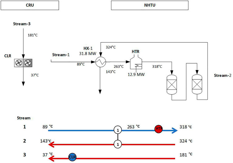
FIGURE 4. HEN configuration before retrofitting.

The proposed heat recovery measure involves adding a new heat exchanger HX-2 which enables Stream 3 from CRU to be used to preheat Stream 1 in NHTU before it enters HX-1. The increased pre-heating provides a higher temperature into the furnace, decreasing the need for fuel gas from 12.9 to 6.2 MW. To maintain the load of HX-1 and thereby the target temperature of Stream 2 (143°C), the heat transfer area of HX-1 needs to be increased to compensate for the decreased temperature difference between the hot and cold stream. The proposed changes to the HEN are shown in Figure 5. Because of spatial restrictions and to enable cleaning of the heat exchanger during operation, a parallel configuration with two plate heat exchangers was retained. Since HX-1 will require two heat exchangers in series as well, three units of equal size (701 m²) are suggested for HX-1, since one parallel is required to enable cleaning. HX-2 is smaller and two parallel heat exchangers (107 m²) are suggested for alternating operation.

FIGURE 5

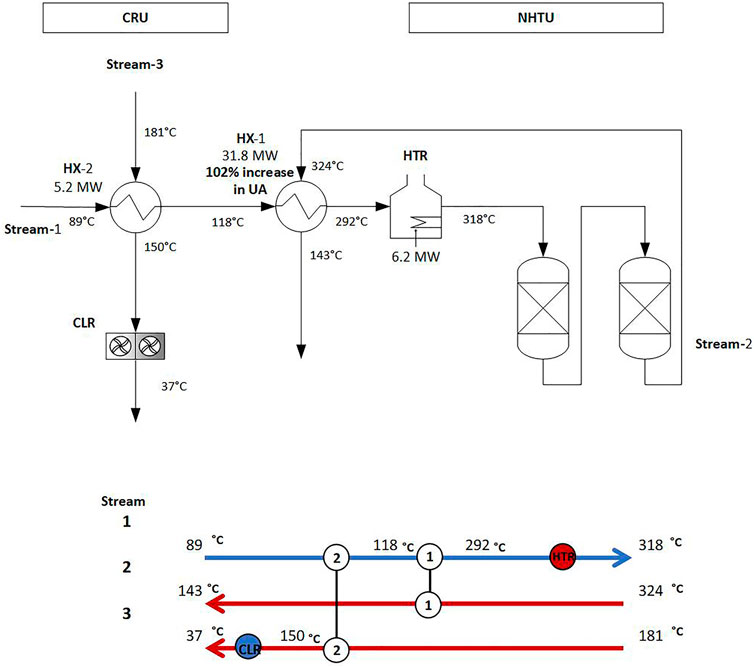
FIGURE 5. HEN configuration after retrofitting.

The conceptual design was derived based on pinch design principles with individual ΔT_min for the streams. These ΔT_min values determine preliminary values for the heat exchanger areas of the conceptual design, as given below. However, when the HEN design is optimized for TAC and flexibility, the ΔT_min values are no longer used The retrofit was discussed with plant engineers to establish a relevant value for the heat transfer coefficient of the new heat exchanger, and to verify that other assumptions were reasonable. Further information about the pinch study can be found in Andersson et al. (2013), Åsblad et al. (2014) and Marton et al. (2020).

Current Operation and Short-Term Variations—Nominal Point 1

One operating point is chosen to represent current, normal operation, see Table 1. Short-term variations were expressed via maximum positive and negative disturbance values (ΔT_start, ΔT_target, and ΔFCp), which indicate the maximum variation around the corresponding nominal values. For this case study, the variation ranges were assumed since historical data was not available. However, since the proposed flexibility ratio is a relative indicator (which unlike the flexibility index does not assign a special limit for feasibility at a flexibility ratio = 1, see Trade-Offs Between Costs and Flexibility), the variation range is not strictly required to represent expected variations, but can still be used to investigate the trade-off between costs and different degrees of flexibility for the retrofit.

TABLE 1

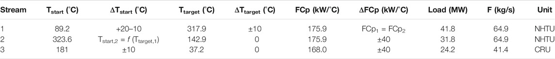
TABLE 1. Operating point representing current operation and assumed variations.

To express the dependency between the reactor inlet temperature (T_target,1) and the reactor outlet temperature (T_start,2) a linear function was assumed. The equation was based on measurement data from the refinery.

$T_{start,2}= 0.793 T_{target,1}+71.547(3)$

Long-Term Development—Nominal Point 2

In order to illustrate the approach presented in this paper for evaluating flexibility with respect to long-term changes due to process development, a scenario was chosen that assumes a future implementation of biomass co-processing that affects the operation of the NHTU. This is based on the possibility of NHTU as being one potential feed-in point for pre-processed biomass feed in existing refineries [see e.g., van Dyk et al. (2019)]. Since this kind of change affects the two process units included in the proposed heat recovery measure differently, it is expected to create an imbalance which could potentially cause flexibility issues for the HEN and limit the production capacity.

Biomass integration would create a new nominal point. This is modeled by assuming that the flows in NHTU are increased by 50%. The new nominal point is shown in Table 2. The same short-term variations as current operations are assumed around this new nominal operating point.

TABLE 2

TABLE 2. Nominal operating point for future operating point with biomass integration.

If the flows of stream 1 and 2 are increased, this could affect the feasibility of a HEN retrofit design. Therefore, it is desirable to consider these future changes in the flexibility analysis of the retrofit, for example, using the methodology proposed in Analyzing Flexibility with Respect to Expected Long-Term Development.

Results

In this section, the results for the case study are presented.

Current Operation—Nominal Point 1

If only short-term variations are considered for the energy efficiency measure, the proposed conceptual design based on pinch analysis has a flexibility ratio of 0.91 (see Step 3, Theoretical Background), which can be seen in Figure 6. This means that it is possible to operate the HEN with variations at least up to 91% of the nominal variation assumed. As shown in the figure, this conceptual design (pinch based without optimization) is not only less flexible than a design optimized to be feasible for nominal variations, but also more expensive. In fact, when the design parameters (i.e., heat exchanger areas) of the proposed HEN structure are optimized with respect to TAC at the nominal point (see Step 4, Theoretical Background), the optimized solution includes larger heat exchangers, which results in higher flexibility (flexibility ratio 1.01) than the original design even if flexibility is not considered in the optimization problem. Consequently, even if a smaller flexibility target is set, the optimum solution will yield a design with this flexibility ratio; the economic trade-off between operating costs (fuel use) and capital cost (heat exchanger area) by itself drives the solution to heat exchanger areas allowing for this degree of flexibility. The increased operating costs associated with increased fuel gas usage resulting from selecting smaller heat exchangers will be higher than the decreased capital cost of the heat exchangers.

FIGURE 6

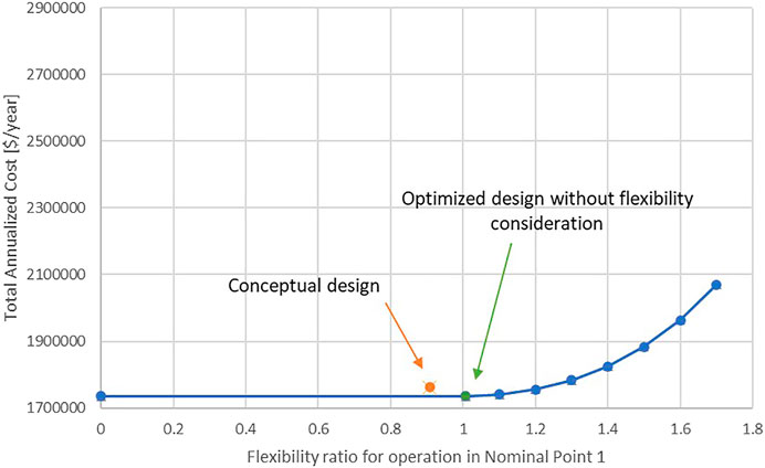
FIGURE 6. Minimum TAC for nominal point 1 for varying flexibility ratio requirements.

Figure 6 also shows the minimum TAC for solutions optimized for higher flexibility ratio targets (see Steps 5 and 6, Theoretical Background). As can be seen in the figure, the TAC increases more rapidly for higher flexibility ratios. This can be explained by the rapid increase in heat exchanger area requirements as the demand for flexibility is increased. With higher flexibility requirements, the heat exchangers should be able to handle more variations in inlet temperatures, including conditions with lower ΔT_min values. As the required heat transfer area increases rapidly with lower temperature driving forces, this has a strong effect on the optimal area. The relation between flexibility ratio and corresponding optimal heat exchanger area is shown explicitly in Table 3. The higher the flexibility ratio required, the greater is the effect of the increased area requirements on capital cost compared to the savings in operating cost from decreased fuel gas use. Note that the areas for both heat exchangers increase when the flexibility requirement is increased.

TABLE 3

TABLE 3. Optimized TAC and resulting areas for HX-1 (3 units) and HX-2 (2 units).

It should also be noted that all investigated nodes on the TAC (flexibility ratio) function are within the structural flexibility limit, meaning it is possible to achieve the desired flexibility ratio with the proposed HEN structure by increasing area in appropriate heat exchangers.

Sensitivity of Derived Solutions to Long-Term Development

For this paper, the same magnitude of nominal short-term variations was used for both nominal points. Since future variations could be hard to predict it is necessary to allow for some uncertainty regarding the flexibility ratio that is required for a future nominal point, i.e., to not define too strictly a fixed flexibility requirement. To avoid specifying a fixed limit for feasible operation, the approach presented in this paper enables a cost comparison over the range of uncertain flexibility ratios for possible future nominal points.

To evaluate how sensitive the relationship between costs and flexibility are to changes in nominal operating conditions, each design representing a node in the original trade-off function TAC (flexibility ratio) for nominal point 1 is re-evaluated in terms of what the flexibility ratio and TAC would be for these designs at nominal operating point 2. Following the approach described in Sensitivity Toward Long-Term Development, each design (corresponding to one node in Figure 6) is fixed, the resulting TAC is evaluated by solving P1 with fixed design parameters but with new operating conditions, and the flexibility ratio is recalculated assuming the new operating point. Figure 7 shows the resulting trade-off between TAC and flexibility ratio for the designs given the new operating point. The resulting TACs are higher for nominal point 2 than for nominal point 1, which since increased mass flow of stream 1 at nominal point 2 creates a higher demand for heating in the furnace, and consequently a higher fuel cost.

FIGURE 7

FIGURE 7. TAC and flexibility ratio for nominal point 2 for nodes optimized for nominal point 1.

Interestingly, the lowest cost is achieved for the design that results in a flexibility ratio of 0.89 for nominal point 2. This design corresponds to the node optimized for flexibility ratio 1.3 for the nominal point 1 in Figure 6. This shows that in the future scenario represented by nominal point 2, the TACs are lower for designs that also allow a higher flexibility ratio (up to a flexibility ratio of around 0.9). In other words, the design (node) that gives the lowest TAC for nominal point 1, is not optimal in terms of either costs or flexibility at nominal operating point 2. Depending on the certainty and timeline for the planned process changes, it could therefore be worth considering to choose a design with higher flexibility (and somewhat higher costs) at nominal point 1, in order to obtain both a more cost-effective solution and better flexibility if and when the process conditions are altered.

Generally, the resulting flexibility ratios for nominal point 2 are lower than for nominal point 1 for the given designs, which were originally derived for nominal point 1. The relation between the flexibility ratios for nominal point 1 and 2 for the investigated nodes and their corresponding designs can be seen in Table 4. This can be used to see how large overdesign (in terms of additional flexibility) would be necessary for a retrofit to reach a certain desired flexibility ratio in a future scenario. For example, if a flexibility ratio of 1.2 or higher is desirable in a future scenario, the retrofit must be designed for a flexibility ratio around 1.5 to 1.6 for nominal point 1.

TABLE 4

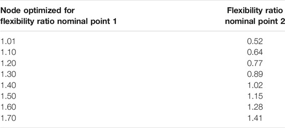
TABLE 4. Flexibility ratio for nodes optimized for Nominal Point 1 and operated at Nominal point 2.

It should be noted that the approach of evaluating flexibility for future operating points could include other process developments like CCS, CCU, electrification or other kinds of biomass integration.

The TAC for nominal point 1 and 2 could be compared to see how cost vs flexibility ratio varies for the two operating scenarios. A similar analysis could also be performed for more than one future scenario. This can be helpful to estimate how costs and flexibility will be affected by possible future operating conditions expected due to long-term development. For this case it is obvious that the flexibility ratio for nominal point 2 determines the overall flexibility ratio for the retrofit.

Optimization for Current and Future Conditions

One component of the TAC of a HEN retrofit design are the operating costs, which vary with operating conditions—internal process conditions as well as external factors such as energy prices. Consequently, if the process is expected to operate under different conditions over the lifetime of the investment, there is a need to consider a suitable weighting of the operating costs.

In Figure 8, three different operating scenarios are presented. All nodes in the graph are optimized for discrete points of overall flexibility ratio (see Overall Flexibility Ratio), while the different lines represent costs optimized for different operating conditions. However, since the overall flexibility ratio represents the minimum range of variations relative to the nominal operating variations around all considered nominal operating points, this means that the optimized solutions (even if optimized for one scenario only) all fulfill the flexibility requirements for both the current and the future nominal operating conditions. The grey/lowest line shows solutions where the design parameters (i.e., heat exchanger areas) are optimized and evaluated for operation at nominal point 1 only (i.e., Step 9a, Economic Calculations), and the blue/top line shows solutions optimized and evaluated for operation at nominal point 2 only (see Step 9b, Economic Calculations). To represent a case where the process is first assumed to be operated during a number of years at nominal point 1, and thereafter shifted to nominal point 2 for remainder of its economic lifetime, a yellow/middle line shows optimized TAC values for a case where operation around each nominal point is given equal weight in the optimization. As previously mentioned, it is a direct result of the assumed process development that the TACs are higher at nominal point 2 since the flow to the furnace is higher, leading to higher operating cost.

FIGURE 8

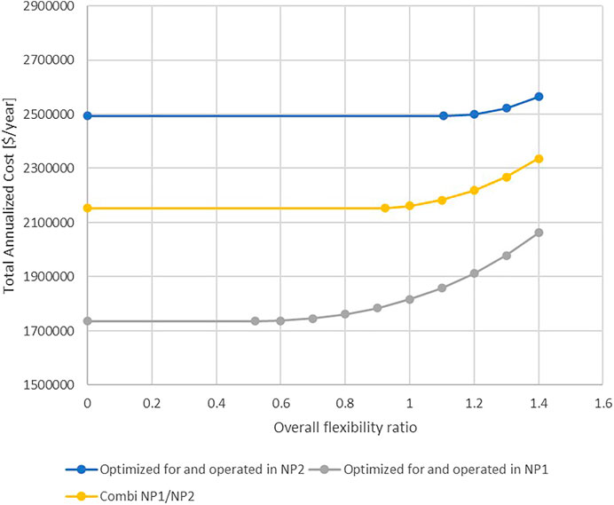
FIGURE 8. Minimized TAC for different overall flexibility ratios for operation at nominal point 1 (grey/lower curve), operation at nominal point 2 (blue/upper curve) and a weighted average between the operating points (yellow/middle curve).

If the retrofit is optimized without flexibility considerations, the overall flexibility ratio for the optimal design varies between the operational cases described above. For operation at nominal point 1, the optimal design without flexibility considerations has an overall flexibility ratio of 0.52 (i.e., this is the lower bound for the overall flexibility ratio at this nominal operating point, see Step 4, Economic Calculations). Here, the overall flexibility ratio is limited by the flexibility of this design at nominal point 2. Note that this node corresponds to the same design as the one optimized without flexibility considerations in Figure 6, which had a flexibility ratio of 1.01 relative to nominal variations around point 1. For the weighted scenario (yellow/middle line), the design optimized without flexibility constraints has an overall flexibility ratio of 0.92 and for operation at nominal point 2 only, the design optimized without flexibility constraints has an overall flexibility ratio of 1.11.

The minimum TAC and optimized heat exchanger area for the discrete nodes illustrated in Figure 8 are shown in Table 5 for the three operating scenarios. The results presented in the table show that the size of heat exchanger 1 determines the overall flexibility ratio for the investigated nodes (the size of the heat exchanger is the same in all operating scenarios for a given flexibility target) while the size of heat exchanger 2 depends on the operating scenario.

TABLE 5

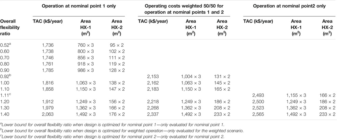
TABLE 5. Minimized TAC and areas for HX-1 (3 units) and HX-2 (2 units) for a designs optimized for operation at nominal point 1, 2 or a weighted average between the operating points.

Even if the results presented above provides an overview of the overall flexibility in the expected operating points for solutions that are optimized for a specific operating scenario, it provides little insights into the cost penalties of optimizing for a scenario that does not in fact occur.

If the retrofit is optimized for operation at nominal point 2 but operated at nominal point 1 the costs will be higher than if the retrofit was optimized for operation at nominal point 1. Such a situation could occur, for example, if the retrofit is optimized for a planned rebuild of the process plant, but the planned changes are canceled or postponed. The resulting cost penalty is displayed as the difference between the curves shown in Figure 9. The grey/lower curve shows solutions optimized and evaluated for operation at nominal point 1 and is the same as the grey/lower curve in Figure 8. The blue/upper curve in Figure 9 is constructed by taking the design parameters corresponding to the nodes from the blue/upper curve in Figure 8, which were optimized for nominal point 2, and evaluating them for operation at nominal point 1. For a given overall flexibility ratio, the difference in cost between the curves represent the cost penalty of optimizing for a process change that does not occur as planned. The cost penalty is larger for lower overall flexibility ratios and small for higher overall flexibility ratios. The designs corresponding to the nodes for flexibility ratio 1.1 and higher consist of quite similar heat exchanger sizes which can be seen in Table 5. For flexibility ratios lower than 1.1, the difference is mainly explained by the fact that the first node represents the lower bound for the overall flexibility ratio in nominal point 2. This implies that lower flexibility ratio targets will not lead to a reduction in costs. To summarize, if the plant is operated at nominal point 1 but optimized for operation at nominal point 2, the heat exchangers will be overdesigned if a lower flexibility ratio is required, leading to a higher TAC than necessary. If a higher flexibility ratio is required, the cost difference is small, and it is of less significance which nominal point the retrofit is optimized for.

FIGURE 9

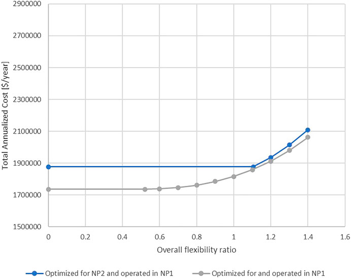
FIGURE 9. Minimized TAC for different overall flexibility ratios for operation at nominal point 1 (grey/lower curve) and nodes minimized for operation at nominal point 2 but evaluated for operation at nominal point 1 (blue/upper curve).

Contrarily to the above example, the retrofit design could be optimized for operation at nominal point 1 but switched to operation at nominal point 2 sooner than planned (e.g., immediately). Similarly to the previous example, the TAC will be higher than if the retrofit would have been optimized for nominal point 2. The cost penalty (additional TAC) is illustrated by the difference between the curves in Figure 10. The blue/lower curve contains solutions that are optimized and evaluated for nominal point 2 and is the same as the blue/upper curve in Figure 8. The grey/upper curve consist of solutions optimized for operation at nominal point 1 (the grey/lower curve in Figure 8), but evaluated for operation at nominal point 2. Here, there appears to be a minimum cost penalty around an overall flexibility ratio of 0.9. This means that as the overall flexibility ratio target is increased above 0.9, the cost penalty of optimizing for a scenario that does not in fact occur (i.e., assuming nominal point 1, but nominal point 2 is the one that actually occurs), is increased. Therefore, it could be beneficial to keep the flexibility target close to 0.9, especially if future process development is uncertain.

FIGURE 10

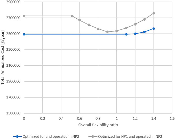
FIGURE 10. Minimized TAC for different overall flexibility ratios for operation at nominal point 2 (blue/lower curve) and nodes minimized for operation at nominal point 1 but evaluated for operation at nominal point 2 (grey/higher curve).

The results presented above can be used to make an informed decision about what overall flexibility ratio to choose for the HEN design and for what nominal point the TAC should be minimized. For example, If a high degree of flexibility is desired because of large uncertainties about the variations affecting the process—today and in the future, there is only a small cost penalty (ranging from 24 to 46 k$/year for overall flexibility ratios between 1.2 and 1.4, see Figure 9) of optimizing the design for nominal point 2, even if the process is then mostly operated in nominal point 1 (as shown by the costs for high overall flexibility ratios in Figure 9). As seen in Table 5, the heat exchangers of the optimized designs are similar in size for a given overall flexibility ratio and the increased cost for minimizing TAC for nominal point 2 could be explained by the slightly larger exchanger area of HX-2. However, if the HEN design is optimized to minimize TAC at nominal point 1, but the process is then operated at nominal point 2, the cost penalty for larger flexibility ratios would be higher (ranging from 119 k$/year to 192 k$/year for overall flexibility ratios between 1.2 and 1.4) since the smaller HX-2 area of such designs would limit the potential pre-heating of the cold process stream before the reactor as the flow through this heat exchanger is increased at nominal point 2. For lower overall flexibility ratios (0.5–1.0), the cost penalty is similar for both nominal points, however, it appears to have a minimum at 0.9 for designs optimized for nominal point 1 but operated at nominal point 2 (see Figure 10). Even when the cost penalty of optimizing for wrong nominal point is smaller for larger flexibility ratios, it is more costly to design the HEN for a larger overall flexibility ratio than necessary. Consequently, flexibility requirements, uncertainty and likely nominal point should all be weighted together to decide on what flexibility ratio to design the HEN for.

The approach could also be used to compare several different nominal points and be weighted for these nominal operating points.

Conclusion

The approach presented in this paper provides increased knowledge about cost and flexibility for HEN retrofits with respect to short-term variations in both current operation and for possible future developments. This paper proposed a flexibility ratio, that can be considered as a key performance indicator for the design of HENs when considering both short-term variations and long-term development. This knowledge can be used to ensure that heat recovery measures are designed to be feasible for long term developments and make informed decisions about how large overdesign will be necessary to achieve certain flexibility requirements for future operating scenarios as well as about the associated cost for the overdesign.

The proposed approach was illustrated for a case study related to enhanced heat recovery measures at an oil refinery. In the case study, the HEN in which the design parameters (heat exchanger areas) were optimized without flexibility considerations (no critical points) not only has a lower TAC, but also a higher flexibility ratio than the conceptual pinch-based design based for all scenarios analyzed. Since the approach is based on optimization it was expected that the costs are lower than a conceptual, non-optimized design, but it was not obvious beforehand that the flexibility for the optimized solutions would be higher. The conceptual design of the HEN retrofit was shown to be flexible/feasible for all operational variations considered and there is no issue with structural flexibility constraints for the investigated flexibility ratio targets. The difference in TAC between the designs derived for different flexibility requirements is significant, but moderate. This implies that it is important to consider flexibility in a decision-making process for this retrofit, but not necessarily at an early design-stage but rather at a more detailed stage of the process. However, it should be noted that for more complicated retrofits or for green-field studies, issues with structural flexibility could arise which should be considered in an earlier design stage. If the retrofit is structurally flexible, the trade-off between heat exchanger area (i.e., cost) and flexibility ratio could be considered later in the design process.

The results show that it could be beneficial to invest in HEN retrofits even if there are long-term developments planned. Additionally, an analysis regarding flexibility ratio and TAC for both short-term variations and long-term development will enable a more accurate picture of how to save carbon emissions and reduce overall costs for future changes. Furthermore, the proposed approach also provides information about the cost penalty incurred for a retrofit measure as a function of the difference between assumed operation point and other possible operating scenarios. This provides guidance for which operational scenario is most important to consider when designing the retrofit.

Future Work

Future work should mainly include more complex case studies to further develop and validate the proposed methodology. This should include larger and more complex HENs as well as a larger variety of alternative future development scenarios. Strategic, long-term, climate mitigation actions are necessary for all refineries with fossil feedstock. Ambitious heat recovery solutions are essential for ensuring a high resource and energy efficiency and maximized utilization of low-carbon resources in the future, decarbonized processes. However, HEN retrofits to enhance heat recovery are also necessary today to decrease climate impact of current fossil-based energy use in existing process. Thus, the approach presented in this paper provides guidelines about how to adapt and “future-proof” HEN retrofits for long-term climate mitigation options. It would be desirable to be able to compare a flexibility ratio for several possible climate mitigation pathways to ensure that HEN retrofits to be implemented within the short-term future will not compromise the possibility to implement larger retrofits in the long-term. This should be further investigated in future work.

Data Availability Statement

The raw data supporting the conclusions of this article will be made available by the authors, without undue reservation.

Author Contributions

SM and CL planned and discussed the studied approach and CL conducted the optimization and calculations. SM designed the retrofit proposal and collected data necessary for the optimization. The results were analyzed and discussed by SM, CL and ES. ES and SH supervised the work. CL wrote the methodology section of the paper; SM wrote the remaining sections of the paper. All text was reviewed and discussed by all authors.

Funding

Funding for this work was provided by the Energy Area of Advance at Chalmers University of Technology.

Conflict of Interest

ES was employed at CIT Industriell Energi AB at the time of the study. CIT Industriell Energi AB is a consulting company specializing in knowledge transfer between academia, industry and government agencies, focusing primarily on efficient and sustainable industrial energy use. It is a wholly owned subsidiary to the foundation Chalmers Industriteknik.

The remaining authors declare that the research was conducted in the absence of any commercial or financial relationships that could be construed as a potential conflict of interest.

Abbreviations

HEN, heat exchanger network; HX, heat exchanger; TAC, total annual cost.

References

Andersson, E., Franck, P.-Å., Åsblad, A., and Berntsson, T. (2013). Pinch Analysis at Preem LYR. Gothenburg: ” Chalmers University of Technology.

Andersson, V., Franck, P.-Å., and Berntsson, T. (2014). Industrial Excess Heat Driven post-combustion CCS: The Effect of Stripper Temperature Level. Int. J. Greenhouse Gas Control. 21, 1–10. doi:10.1016/j.ijggc.2013.11.016

CrossRef Full Text | Google Scholar

Andersson, V., Franck, P.-ÿ., and Berntsson, T. (2016). Techno-economic Analysis of Excess Heat Driven post-combustion CCS at an Oil Refinery. Int. J. Greenhouse Gas Control. 45, 130–138. doi:10.1016/j.ijggc.2015.12.019

CrossRef Full Text | Google Scholar

Arbogast, S., Bellman, D., Paynter, J. D., and Wykowski, J. (2012). Advanced Bio-Fuels from Pyrolysis Oil: The Impact of Economies of Scale and Use of Existing Logistic and Processing Capabilities. Fuel Process. Tech. 104, 121–127. doi:10.1016/j.fuproc.2012.04.036

CrossRef Full Text | Google Scholar

Arellano-Garcia, H., Ketabchi, E., and Ramirez Reina, T. (2017). “Integration of Bio-Refinery Concepts in Oil Refineries,” in 27th European Symposium on Computer Aided Process Engineering. Editors Pt. A. A. Espuna, M. Graells, and L. Puigjaner, 40A, 829–834. doi:10.1016/b978-0-444-63965-3.50140-9

CrossRef Full Text | Google Scholar

Åsblad, A., AnderssonErikssonFranckSvensson, E. K. P.-Å. E., and Harvey, S. (2014). Pinch Analysis at Preem LYR II Modifications. Gothenburg: Chalmers University of Technology.

Bakar, S. H. A., Hamid, M. K. A., Alwi, S. R. W., and Manan, Z. A. (2016). Selection of Minimum Temperature Difference (ΔTmin) for Heat Exchanger Network Synthesis Based on Trade-Off Plot. Appl. Energ. 162, 1259–1271. doi:10.1016/j.apenergy.2015.07.056

CrossRef Full Text | Google Scholar

Berghout, N., Meerman, H., van den Broek, M., and Faaij, A. (2019). Assessing Deployment Pathways for Greenhouse Gas Emissions Reductions in an Industrial Plant - A Case Study for a Complex Oil Refinery. Appl. Energ. 236, 354–378. doi:10.1016/j.apenergy.2018.11.074

CrossRef Full Text | Google Scholar

Biermann, M., Langner, C., Eliasson, Å., Normann, F., Harvey, S., and Johnsson, F. (2021). “Partial Capture from Refineries through Utilization of Existing Site Energy Systems,” in 15th International Conference on Greenhouse Gas Control Technologies (Abu Dhabi, UAE. GHGT-15 15th-18th March 2021.

Google Scholar

Bütün, H., Kantor, I., and Marechal, F. (2019). Incorporating Location Aspects in Process Integration Methodology. Energies 12 (17), 3338. doi:10.3390/en12173338

CrossRef Full Text | Google Scholar

Chew, K. H., Klemeš, J. J., Abdul Manan, S. R. Z., and Manan, Z. A. (2013). Industrial Implementation Issues of Total Site Heat Integration. Appl. Therm. Eng. 61 (1), 17–25. doi:10.1016/j.applthermaleng.2013.03.014

CrossRef Full Text | Google Scholar

European Comission. (2018). "Energy Efficiency." Retrieved from https://ec.europa.eu/energy/en/topics/energy-efficiency [ [12 October 2020].

Google Scholar

Fernández-Dacosta, C., Stojcheva, V., and Ramirez, A. (2018). Closing Carbon Cycles: Evaluating the Performance of Multi-Product CO2 Utilisation and Storage Configurations in a Refinery. J. Co2 Utilization 23, 128–142. doi:10.1016/j.jcou.2017.11.008

CrossRef Full Text | Google Scholar

Fleiter, T., Hirzel, S., and Worrell, E. (2012). The Characteristics of Energy-Efficiency Measures - a Neglected Dimension. Energy Policy 51, 502–513. doi:10.1016/j.enpol.2012.08.054

CrossRef Full Text | Google Scholar

FuelsEurope (2018). Vision 2050 A Pathway for the Evolution of Refining Industry and Liquid Fuels. Retrieved 2021-03-08.

Grossmann, I. E., and Floudas, C. A. (1987). Active Constraint Strategy for Flexibility Analysis in Chemical Processes. Comput. Chem. Eng. 11 (6), 675–693. doi:10.1016/0098-1354(87)87011-4

CrossRef Full Text | Google Scholar

Grossmann, I. E., Halemane, K. P., and Swaney, R. E. (1983). Optimization Strategies for Flexible Chemical Processes. Comput. Chem. Eng. 7 (4), 439–462. doi:10.1016/0098-1354(83)80022-2

CrossRef Full Text | Google Scholar

Hackl, R., and Harvey, S. (2015). From Heat Integration Targets toward Implementation - A TSA (Total Site Analysis)-Based Design Approach for Heat Recovery Systems in Industrial Clusters. Energy 90, 163–172. doi:10.1016/j.energy.2015.05.135

CrossRef Full Text | Google Scholar

Hafizan, A. M., Alwi, S. R. W., Abd Manan, Z., Klemes, J. J., and Abd Hamid, M. K. (2020). Design of Optimal Heat Exchanger Network with Fluctuation Probability Using Break-Even Analysis. Energy 212, 118583. doi:10.1016/j.energy.2020.118583

CrossRef Full Text | Google Scholar

Hiete, M., Ludwig, J., and Schultmann, F. (2012). Intercompany Energy Integration. J. Ind. Ecol. 16 (5), 689–698. doi:10.1111/j.1530-9290.2012.00462.x

CrossRef Full Text | Google Scholar

Jafri, Y., Wetterlund, E., Anheden, M., Kulander, I., Furusjö, Å., and Furusjo, E. (2019). Multi-aspect Evaluation of Integrated forest-based Biofuel Production Pathways: Part 1. Product Yields & Energetic Performance. Energy 166, 401–413. doi:10.1016/j.energy.2018.10.008

CrossRef Full Text | Google Scholar

Jafri, Y., Wetterlund, E., Anheden, M., Kulander, I., Furusjö, Å., and Furusjo, E. (2019a). Multi-aspect Evaluation of Integrated forest-based Biofuel Production Pathways: Part 2. Economics, GHG Emissions, Technology Maturity and Production Potentials. Energy 172, 1312–1328. doi:10.1016/j.energy.2019.02.036

CrossRef Full Text | Google Scholar

Jegla, Z., and Freisleben, V. (2020). Practical Energy Retrofit of Heat Exchanger Network Not Containing Utility Path. Energies 13 (11), 2711. doi:10.3390/en13112711

CrossRef Full Text | Google Scholar

Kachacha, C., Zoughaib, A., and Tran, C. T. (2018). A Methodology for the Flexibility Assessment of Site Wide Heat Integration Scenarios. Energy 154, 231–239. doi:10.1016/j.energy.2018.04.090

CrossRef Full Text | Google Scholar

Kang, L., and Liu, Y. (2019). Synthesis of Flexible Heat Exchanger Networks: A Review. Chin. J. Chem. Eng. 27 (7), 1485–1497. doi:10.1016/j.cjche.2018.09.015

CrossRef Full Text | Google Scholar

Kantor, I., Robineau, J. L., Butun, H., and Marechal, F. (2020). A Mixed-Integer Linear Programming Formulation for Optimizing Multi-Scale Material and Energy Integration. Front. Energ. Res. 8, 49. doi:10.3389/fenrg.2020.00049

CrossRef Full Text | Google Scholar

Lal, N. S., Atkins, M. J., Walmsley, T. G., Walmsley, M. R. W., and Neale, J. R. (2019). Flexibility Analysis of Heat Exchanger Network Retrofit Designs Using Monte Carlo Simulation. Chem. Eng. Trans. 76, 463–468.

Google Scholar

Langner, C., Svensson, E., and Harvey, S. (2021). A Computational Tool for Guiding Retrofit Projects of Industrial Heat Recovery Systems Subject to Variation in Operating Conditions. Appl. Therm. Eng. 182. doi:10.1016/j.applthermaleng.2020.115648

CrossRef Full Text | Google Scholar

Langner, C., Svensson, E., and Harvey, S. (2020). A Framework for Flexible and Cost-Efficient Retrofit Measures of Heat Exchanger Networks. Energies 13 (6), 1472. doi:10.3390/en13061472

CrossRef Full Text | Google Scholar

Li, J., Du, J., Zhao, Z., and Yao, P. (2014). Structure and Area Optimization of Flexible Heat Exchanger Networks. Ind. Eng. Chem. Res. 53 (29), 11779–11793. doi:10.1021/ie501278c

CrossRef Full Text | Google Scholar

Liu, L., Bai, Y., Zhang, L., Gu, S., and Du, J. (2019). Synthesis of Flexible Heat Exchanger Networks Considering Gradually Accumulated Deposit and Cleaning Management. Ind. Eng. Chem. Res. 58 (27), 12124–12136. doi:10.1021/acs.iecr.9b01672

CrossRef Full Text | Google Scholar

Marselle, D. F., Morari, M., and Rudd, D. F. (1982). Design of Resilient Processing Plants-II Design and Control of Energy Management Systems. Chem. Eng. Sci. 37 (2), 259–270. doi:10.1016/0009-2509(82)80160-7

CrossRef Full Text | Google Scholar

Marton, S., Svensson, E., and Harvey, S. (2020). Operability and Technical Implementation Issues Related to Heat Integration Measures-Interview Study at an Oil Refinery in Sweden. Energies 13 (13), 3478. doi:10.3390/en13133478

CrossRef Full Text | Google Scholar

Marton, S., Svensson, E., Subiaco, R., Bengtsson, F., and Harvey, S. (2017). A Steam Utility Network Model for the Evaluation of Heat Integration Retrofits - A Case Study of an Oil Refinery. J. Sustain. Dev. Energy Water Environ. Syst. 5 (4), 560–578. doi:10.13044/j.sdewes.d5.0167

CrossRef Full Text | Google Scholar

Naturvårdsverket (2018). Utsläpp I Siffror. Stockholm. Available at: https://utslappisiffror.naturvardsverket.se (Accessed March 15, 2020).

Google Scholar

Ochoa, M. P., and Grossmann, I. E. (2020). Novel MINLP Formulations for Flexibility Analysis for Measured and Unmeasured Uncertain Parameters. Comput. Chem. Eng. 135, 106727. doi:10.1016/j.compchemeng.2020.106727

CrossRef Full Text | Google Scholar

Payet, L., Thery Hétreux, R., Hétreux, G., Bourgeois, F., and Floquet, P. (2018). Flexibility Assessment of Heat Exchanger Networks: From a Thorough Data Extraction to Robustness Evaluation. Chem. Eng. Res. Des. 131, 571–583. doi:10.1016/j.cherd.2017.11.036

CrossRef Full Text | Google Scholar

Pintaric, Z. N., and Kravanja, Z. (2008). Identification of Critical Points for the Design and Synthesis of Flexible Processes. Comput. Chem. Eng. 32 (7), 1603–1624.

Google Scholar

Setiawan, R., and Bao, J. (2011). Analysis of Interaction Effects on Plantwide Operability. Ind. Eng. Chem. Res. 50 (14), 8585–8602. doi:10.1021/ie1025198

CrossRef Full Text | Google Scholar

Sharifzadeh, M., Sadeqzadeh, M., Guo, M., Borhani, T. N., Murthy Konda, N. V. S. N., Garcia, M. C., et al. (2019). The Multi-Scale Challenges of Biomass Fast Pyrolysis and Bio-Oil Upgrading: Review of the State of Art and Future Research Directions. Prog. Energ. Combustion Sci. 71, 1–80. doi:10.1016/j.pecs.2018.10.006

CrossRef Full Text | Google Scholar

Smith, R., Jobson, M., and Chen, L. (2010). Recent Development in the Retrofit of Heat Exchanger Networks. Appl. Therm. Eng. 30 (16), 2281–2289. doi:10.1016/j.applthermaleng.2010.06.006

CrossRef Full Text | Google Scholar

Sreepathi, B. K., and Rangaiah, G. P. (2014). Review of Heat Exchanger Network Retrofitting Methodologies and Their Applications. Ind. Eng. Chem. Res. 53 (28), 11205–11220. doi:10.1021/ie403075c

CrossRef Full Text | Google Scholar

Svensson, E., Morandin, M., Harvey, S., and Papadokonstantakis, S. (2020). Studying the Role of System Aggregation in Energy Targeting: A Case Study of a Swedish Oil Refinery. Energies 13 (4), 958. doi:10.3390/en13040958

CrossRef Full Text | Google Scholar

Swaney, R. E., and Grossmann, I. E. (1985). An index for Operational Flexibility in Chemical Process Design. Part I: Formulation and Theory. Aiche J. 31 (4), 621–630. doi:10.1002/aic.690310412

CrossRef Full Text | Google Scholar

van Dyk, S., Su, J., McMillan, J. D., and Saddler, J. (2019). Potential Synergies of Drop‐in Biofuel Production with Further Co‐processing at Oil Refineries. Biofuels, Bioprod. Bioref. 13 (3), 760–775. doi:10.1002/bbb.1974

CrossRef Full Text | Google Scholar

Wang, B. H., Klemes, J. J., Li, N. Q., Zeng, M., Varbanov, P. S., and Liang, Y. T. (2021). Heat Exchanger Network Retrofit with Heat Exchanger and Material Type Selection: A Review and a Novel Method. Renew. Sust. Energ. Rev. 138, 110479. doi:10.1016/j.rser.2020.110479

CrossRef Full Text | Google Scholar

Wiertzema, H., Svensson, E., and Harvey, S. (2020). Bottom-Up Assessment Framework for Electrification Options in Energy-Intensive Process Industries. Front. Energ. Res. 8, 192. doi:10.3389/fenrg.2020.00192

CrossRef Full Text | Google Scholar