Online Internal Temperature Sensors in Lithium-Ion Batteries: State-of-the-Art and Future Trends

1 Introduction

A vehicle battery may be operated in various weather conditions including both hot and cold conditions. Further, while in use, heat is generated inside the battery due to electrochemical reactions and resistances. The internal temperature is an important ageing accelerator which then influences the battery capacity and power characteristics. Some of the ageing effects are lithium plating, solid electrolyte interphase (SEI) growth, loss of cyclable lithium and particle cracks (Waldmann et al., 2014). Moreover, at high internal temperatures the risk of safety hazards such as thermal runaway, venting, fire or explosions are higher. Figure 1A shows various stages of thermal runaway. While increased temperature accelerates the ageing of LIB above 30°C, once the battery reaches temperature higher than 85°C more critical reaction pathways start being triggered (Yang et al., 2006). The SEI on the carbon anode starts decomposing exothermically when the temperature rises above 85°C. Due to the incomplete SEI, the negative electrode material starts reacting exothermically with the solvent at temperatures near 100–110°C. Some of the released heat might lead to evaporation of the electrolyte and melting of the separator (130–190°C). This again leads to further problems like combustion of the organic electrolyte if oxygen is available from the delithiated positive electrode. The positive electrode can either react with the electrolyte directly or evolve oxygen that reacts with the electrolyte. A melted separator triggers short-circuits and therefore additional heating. The negative electrode reacts at 330°C, releasing additional heat. Eventually the aluminum current collector can be melted at 660°C if an explosion has not occurred first (Yang et al., 2006; Bandhauer et al., 2011; Waldmann et al., 2014). Therefore, for safe operation of the battery, proper monitoring and controlling of internal temperature is a key factor.

FIGURE 1

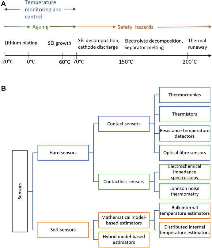
FIGURE 1. (A) The influence of temperature on the battery and the importance of temperature control. (not to scale) (B) Categorization of various sensor types.

Internal thermal sensing is a broad area with different methods where some techniques are well established while others still require development. These sensing methods can be categorized into “hard sensors” and “soft sensors”: hard sensors are hardware-based sensors, measurement systems, or data acquisition systems that can measure the internal temperature directly or indirectly. This includes the sensors that need to be inserted into the cell (contact sensors) and other non-intrusive, non-invasive sensors that can infer the internal temperature (contactless sensors). Soft sensors are estimators or observers that can estimate the internal temperature using various types of models based on other measurements such as the surface temperature, voltage and current.

In recent reviews, most of the hard sensors that are commonly used in battery management systems (BMS) are presented by Srinivasan et al. (2020); Liu et al. (2019); Xiong et al. (2018), while Raijmakers et al. (2019); Ma et al. (2018) discussed various hard sensors used in lithium-ion batteries (LIBs), and Liao et al. (2019) summarized thermal runaway monitoring techniques. Although there are individual studies that are done on soft sensing in LIBs, there are no reviews on soft sensors for LIBs known to the authors. LIB technology is moving towards smart technology, consequently soft sensors are expected to have increased applicability in the near future combined with state-of-the-art hard sensors. Therefore, an up-to-date literature survey is needed on both hard and soft sensors for LIBs and the main objective of this review is to provide a comprehensive overview of state-of-the-art internal temperature sensors that are used in LIBs. As there are a few existing reviews on hard sensors, the section on hard sensors is kept succinct with lists of various types of hard sensors updated with the most recent studies. More weight is given to the soft sensors focusing on different types of models and estimation methods used. The categorization and the types of sensors that are used in the study are shown in Figure 1B. The literature collection comprehensively summarises relevant studies within the last 5years and some of the older, yet highly relevant studies. For the soft sensors, only explicit internal temperature estimation studies are considered, excluding other estimations such as state-of-charge (SOC), state-of-health (SOH), or thermal runaway.

The paper is organized as follows, where section 2 lists various hard sensor types and their advantages and disadvantages, while section 3 discusses different types of soft sensors, their challenges, benefits, and accuracies. Then the future trends in online internal temperature sensing are presented in section 4, and finally, the conclusions that are drawn from the review are presented in section 5.

2 Hard Sensors

Hard sensors can further be categorized based on the type of the hard sensors, namely contact sensors and contactless (non-intrusive and non-invasive) sensors. Contact sensors (eg., thermocouples, thermistors, fibre optic sensors) are placed inside the cell and directly measure the internal temperature, while the contactless sensors (eg., electrochemical impedance spectroscopy) are non-destructive and do not require placing inside as they measure the internal temperature indirectly. Commonly used contact and contactless sensor types and their typical challenges and benefits are discussed in this section. When comparing sensors more focus in general, is given to the accuracy (closeness of the measurand to the true value) than precision (reproducibility of measurands) unless it is mentioned specifically. For hard sensor accuracy, the rated accuracy of sensor is considered together with the temperature difference between in and out of the cell when applicable.

2.1 Contact Sensors

Typical contact sensors that are used in LIBs are thermocouples, thermally sensitive resistors, resistance temperature detectors (RTD), or optical fiber sensors. The RTD and the thermocouples are the most commonly used sensors in commercial batteries for internal temperature measurements (Wei et al., 2021).

2.1.1 Thermocouples

Thermocouples are one of the most well-utilized sensors in industry due to the low cost, portable size, wide measurement range (−200–2500°C), adequate sensitivity, robustness, and fast response (Childs et al., 2000; Duff and Towey, 2010). Therefore, thermocouples have been widely used in commercial batteries for both surface temperature measurements and internal temperature measurements (Raijmakers et al., 2019). The dependency on a reference temperature, susceptibility to corrosion, and noise are some of the disadvantages of thermocouples (Duff and Towey, 2010).

Some of the details of the thermocouple sensor-based temperature measurement studies are listed in Table 1. This includes the thermocouple type, measured temperature (T) range of the study, the temperature (ΔT) difference recorded between the internal and surface temperature and any other important remarks of the study. Additional studies that used thermocouples for validating soft sensors are not included here as they are mentioned in section 3. The most widely used thermocouple types are K or T type, where N (Hofmann et al., 2017), J (Xiao, 2015) or E (Al Hallaj et al., 1999) types are less frequently used.

TABLE 1

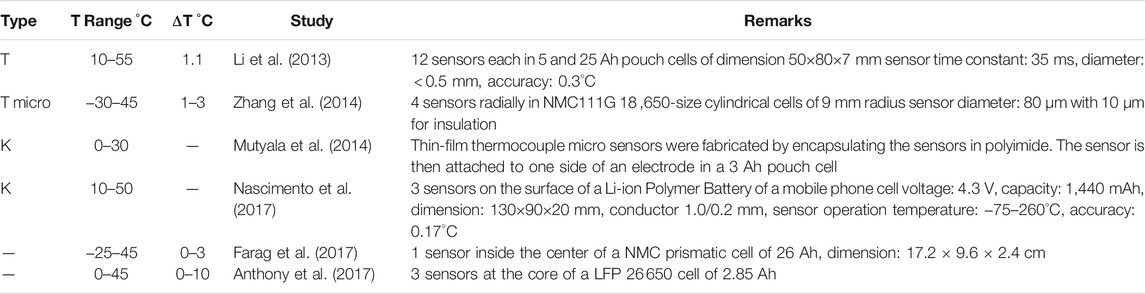
TABLE 1. Details on thermocouple sensors used in LIBs.

2.1.2 Thermally Sensitive Resistors (Thermistors)

Thermally sensitive resistors are more commonly known as thermistors that are variable resistors where its resistance responds to the surrounding temperature. These have a wide measurement range (−55–300°C) and are widely used and considered as low cost, small in size, and highly sensitive to the temperature (Wei et al., 2021). Thermistors are one of the very few sensor types that are used for monitoring in commercially available BMSs, especially in the Toyota Prius and Honda Civic hybrid vehicles (Cao and Emadi, 2011).

There are two types of thermistors, positive temperature coefficient (PTC) and negative temperature coefficient (NTC). When the temperature increases, the resistance of PTC will increase while the resistance of NTC will decrease. NTC thermistors are widely used as these have high precision, near-linear beta curve (temperature versus resistance), wide availability, and a temperature range of −20–120°C (Fleming et al., 2019). Although thermistors are widely used in battery applications, their use in research studies is low. Some of the details of the thermistor-based temperature measurement studies of LIBs are listed in Table 2.

TABLE 2

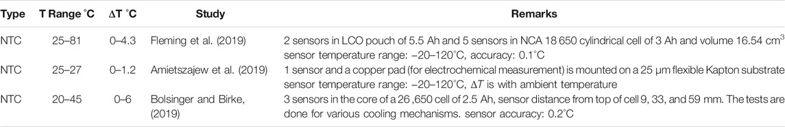
TABLE 2. Details on thermistors used in LIBs.

An embedded thermistor and the cell setup can be seen in Figure 2. Here, the raw thermistor sensors were bonded into a 25 μm flexible Kapton tape that acts as a substrate for the thermistor elements. A protective coating (1 μm thickness) of Parylene was applied to both the thermistor and the substrate before bonding. This was to increase the lifetime of the devices inside the harsh environment of the battery cell. This approach has provided stable measurements and the devices have lasted more than 3 months without any adverse effect on the sensor performance (Fleming et al., 2019).

FIGURE 2

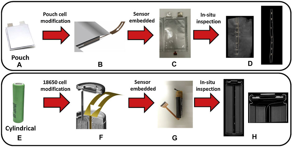
FIGURE 2. Thermistor sensors embedded into pouch and cylindrical cells (Fleming et al., 2019; Panel 5, p. 41). (A) the pouch cell, (E) the cylindrical cell, (B,F) sensor inserted in the cell, (C,G) complete instrumented cell, (D,H) in-situ X-ray images of the cells post-modification, (CC BY-NC-ND 4.0).

2.1.3 Resistance Temperature Detectors

Resistance temperature detectors (RTD) use metallic conductors where the temperature-dependent electric resistance is used for temperature measurement. RTDs have been widely used in commercial batteries, mainly for surface temperature measurements (Wei et al., 2021). Chalise et al. (2017) attached Pt-100 RTD sensors to the poles of 18 ,650 cells, and Chen et al. (2021) mounted Pt-1000 sensors on a 2.3 Ah 26 ,650 cylindrical cell, for surface temperature measurements. Similarly, Wang et al. (2016) used a Pt-1000 sensor (of size 2.3 mm× 2.0 mm) of 0.9 mm of thickness and a measuring range of −50–400°C inside a coin cell as shown in Figure 3. The coin cells are LMO, CR2032 type with a Pt-500 sensor mounted on the surface for the surface temperature. For the protection of the sensor, the copper foil and the sensor were covered by a 50 μm polyimide foil, as polyimide is electrically and chemically inert. The tests were carried out at an ambient temperature of 26°C, where the temperature difference of the measured inside and surface temperatures are in the range of 0–0.08°C under various C rates.

FIGURE 3

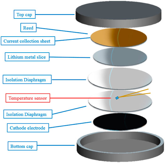
FIGURE 3. A Pt-1000 RTD sensor in a coin cell (Wang et al., 2016, Panel 4, p. 462). Reprinted from (Wang et al., 2016), Copyright (2016) with permission from Elsevier.

A gold RTD type flexible micro sensor was fabricated on a parylene thin film and placed inside a battery for internal temperature measurement by Lee et al. (2011). The parylene acts as a protective layer, an isolation layer, and a substrate. The temperatures were measured in the range of 0–90°C where the temperature differences between inside and surface temperatures were in the range of 0–2°C. Martiny et al. (2014) have also used an RTD sensor-based sensor array for in-situ monitoring of batteries. Another thin film sensor was fabricated by Zhu S. et al. (2020) using a platinum RTD sensor, due to the platinum sensors’ good stability, high accuracy, linear behavior, and wide operating temperature range (−260–960°C). A 20 μm polyimide foil was used as the flexible substrate and the cover layer. An array of 7 sensors is made by depositing the platinum onto the flexible substrates to form seven measuring points where each measuring point was 5 × 5 mm in size and 5 mm distance from each other. The sensors were then inserted into a NMC532 pouch cell, and the measured temperature range is 25–35°C. The temperature difference between the sensors was 1°C which suggests near uniform temperature development along the spatial direction of the layer inside the cell. Similarly, Parekh et al. (2020) have developed internal sensors using RTD sensors and placed them inside an LCO CR2032 coin cell. A Pt-1000 sensor of 4 × 5 mm was placed in a 3D-printed spacer composed of polylactic acid and the assembly was placed behind the current collector of the anode. The temperature measurements ranged between 24 and 38°C, while the maximum temperature difference between internal and surface temperatures was 8.8°C.

2.1.4 Optical Fiber Sensors

The application of optical fiber sensors for battery temperature measurement is an emerging technology in recent years. This is mainly due to the properties such as multi-functionality, fast thermal response, low transmission loss, high optical damage threshold, and low optical non-linearity of the optical fibers (Kersey, 1996; Kashyap, 1999). The glass fibers are electrically and chemically inert, which further explains the interest in these sensors towards internal battery sensing.

The most commonly used optical fiber sensors are the fiber Bragg grating (FBG) sensors (Kersey et al., 1997), due to their quasi-distributed sensing capabilities (Cheng and Pecht, 2017). The grating has a strong reflectivity at a certain wavelength, where it is sensitive to the environment. The grating encodes an absolute wavelength to be reflected to the light detector without dependence on total light levels, losses in the connecting fibers, and couplers or source power. Secondly, they have a quasi-distributed sensing capability where each FBG sensor is assigned a different section of the available source spectrum, which can be used to conduct wavelength division multiplexing in an optical fiber sensing network. A possible solution to the challenges related to the cross-sensitivity between temperature and strain in FBG sensors was investigated by Nascimento et al. (2019), who could decouple the two parameters by creating a Fabry-Perot cavity with different sensitivities in close proximity to the FBG.

Fully distributed sensing can also be realized by measuring backscattered light (Rayleigh, Brilluoin, Raman) in conventional optial fibers, where the position in the fiber is determined either through a time-of-flight principle or by applying a Fourier transform in the frequency domain (Rogers, 1999; Yuksel et al., 2009). This technique was applied by Vergori and Yu (2019) to measure continuous temperature and strain profiles along the surface of a LIB.

Some of the details of the fiber optical sensor-based temperature measurement studies of LIBs are listed in Table 3. Different FBGs are used with single or multi mode fibers, and the most widely used material is silica, that determines the measurable temperature (range) (Raijmakers et al., 2019). Only one study (known to the authors) has tested at sub-zero temperatures (Fortier et al., 2017), which needs to be improved, especially for LIB usage in colder climates. Figure 4 displays the methods used for internal and external incorporation of FBG-based sensors for LIB temperature measurements.

TABLE 3

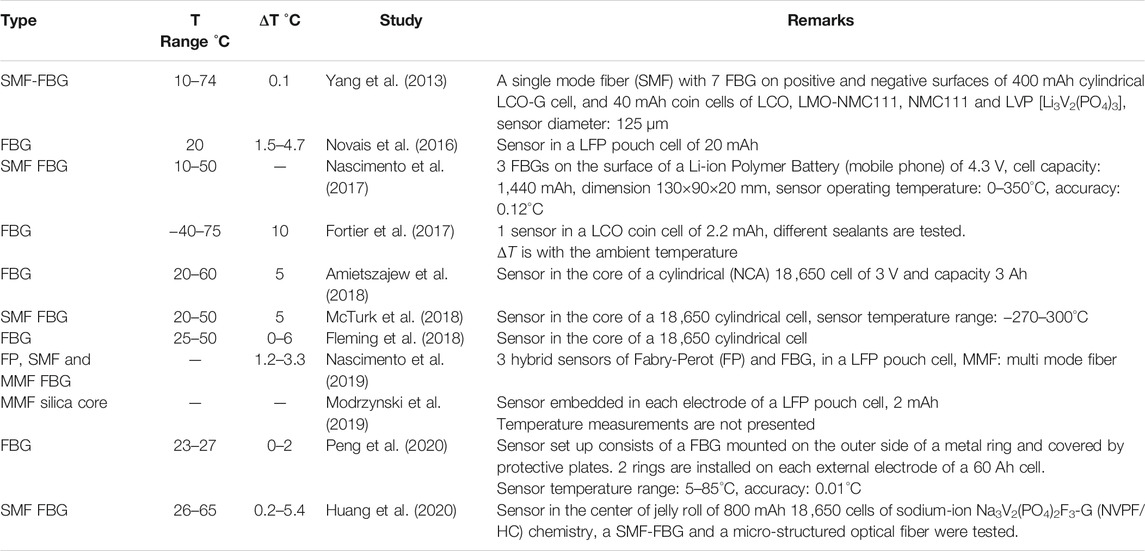
TABLE 3. Details on optical fiber sensors used in cells.

FIGURE 4

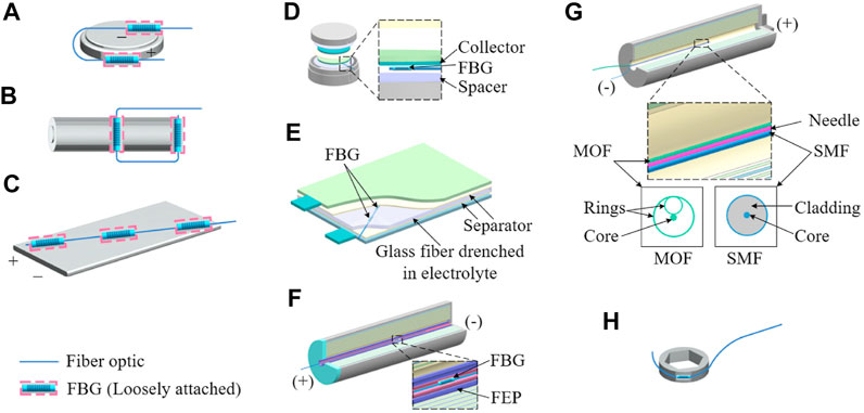
FIGURE 4. FBG sensors on the surface and inside various cell types (Wei et al., 2021; Panel 6, p. 15). (A) FBG on coin cells and (B) FBG on a cylindrical cell (Yang et al., 2013), (C) FBG on a prismatic cell (Nascimento et al., 2017), (D) FBG in a coin cell (Fortier et al., 2017), (E) FBG in a pouch cell, (F) FBG in a cylindrical cell (Amietszajew et al., 2018; Fleming et al., 2018; McTurk et al., 2018), (G) FBG in a cylindrical cell (Huang et al., 2020), (H) FBG in a coin cell (Peng et al., 2020). Reprinted from (Wei et al., 2021), Copyright (2021) with permission from Elsevier.

The variations of the temperature difference between internal and surface temperature for each sensor type shows the importance of the internal temperature monitoring. Further, it also shows that the internal temperature changes due to many factors such as the cell type, ambient temperature, and charging/discharging conditions.

2.2 Contactless Sensors (Non-Destructive Sensors)

Typical contactless sensors that are used in LIBs are electrochemical impedance spectroscopy (EIS), Johnson noise thermometry (JNT), thermal imaging and liquid crystal thermography. These are also known as non-destructive sensors. EIS and JNT are used for internal temperature measurements, while thermal imaging and liquid crystal thermography are mostly used for surface temperature distribution measurement or hot spot detection (Khan et al., 2017; Raijmakers et al., 2019). Only the internal temperature measurement techniques are discussed here.

2.2.1 Electrochemical Impedance Spectroscopy

EIS is commonly used in kinetic and transport property extraction in electrode materials, in aging, modeling and SOC/SOH estimation studies (Waag et al., 2013; Xie et al., 2014; Westerhoff et al., 2016; Zhou and Huang, 2020; Babaeiyazdi et al., 2021). Further, EIS is also used as an internal temperature inference method by relating impedance parameters to the temperature.

Srinivasan et al. (2011) used the EIS method in three different cells (2.3, 4.4, and 53 Ah), utilizing the relationship of the internal temperature with phase shift between an applied sinusoidal current and the resulting voltage, which is a measurable electric parameter. The impedance and the phase shift were measured at a span of frequencies throughout a temperature range of −20–66°C. These measurements were used to derive the electrolyte and separator resistance and the resistance of the SEI layer, which are then used to monitor the internal temperature.

The same principle was extended by Schmidt et al. (2013) to measure internal temperature of a commercial 2 Ah pouch cell. The accuracy of the internal temperature measurement at isothermal conditions is stated as ± 0.17°C when the SOC is known and ±2.5°C when SOC is unknown. Further, Richardson et al. (2014); Richardson and Howey (2015); Richardson et al. (2016a) have used EIS for surface temperature measurements and developed soft sensors to estimate the internal temperature, which are explained in Section 3 in detail.

2.2.2 Johnson Noise Thermometry

JNT uses thermal fluctuations in conductors to measure the temperature. In the JNT technique, both the resistance measurement of the conductor and the power spectral density of the thermal noise are used to determine the temperature. The variation of the resistance of the sensing conductor is representative of the changes in structural and material properties due to harsh environmental effects such as oxidation, corrosion, and vibration. Since this is already included in the JNT temperature measurement, JNT is applicable for harsh environments such as nuclear reactors and electrochemical batteries, where the sensors may significantly degrade over time (Childs et al., 2000; Liu X. et al., 2018).

A JNT method for electric vehicle batteries (tested on a lead-acid battery not on LIB) is proposed by Liu X. et al. (2018), by using a giant magneto resistance (GMR) sensor as the sensing resistor. This GMR-based JNT can operate even when the GMR sensor is subjected to external magnetic fields, as the temperature measurement is independent of the magnetic parameters of the GMR sensor. The temperature sensor was tested in the range of −40–150°C and the measurements were compared with type K thermocouple and platinum RTD measurements. The absolute measuring error of JNT temperature and the reference measurements for two different tests were within the range of −1.42 and 1.76°C and −1.37 and 1.83°C. During the dynamic performance of the lead-acid battery test the absolute error was −2.67 and 3.08°C. The tests were carried out to measure the surface temperature of the battery cells (Liu X. et al., 2018). This method has been used to measure the surface temperature, and although the measurement error is up to 3°C, it has a good future potential for estimating internal temperature.

The contactless methods have the advantage of operating outside the cell without the need to insert into the battery for measuring the internal temperature. However, these are at the research and development stage and have not been proven on an industrial scale (Raijmakers et al., 2019).

2.3 Common Challenges and Benefits of Hard Sensors

One major benefit of embedded sensors is that they can give high-fidelity and reliable benchmark values for internal temperatures, especially for thermal model validations and thermal model-based SOC, SOH estimations (Wei et al., 2021). Another advantage is that it can be highly useful in fast detection of thermal runaway events. It could be too late if thermal runaway detection is only based on the surface temperature measurements as the internal temperature can increase rapidly even though the surface temperature changes slowly.

The contact sensors need to be inserted into the cells, making this method a destructive method. One major challenge is to insert the sensors without damage to the cell and with no loss of the electrolyte. This is not a problem when the sensors are inserted during the manufacturing stage as shown by Amietszajew et al. (2019). However, in the research and development stage, this is a challenge as most researchers use already assembled commercial cells. In that case, various setups have been tested for sensor installing. One such installation done by McTurk et al. (2018), is shown in Figure 5A.

FIGURE 5

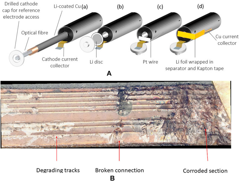
FIGURE 5. Common challenges of hard sensors. (A) Sealing configurations of a cylindrical cell with an embedded thermo-electrochemical sensor (McTurk et al., 2018; Panel 2, p. 311). (B) A microscopic image of a damaged thermistor due to the harsh environment of the cell (Fleming et al., 2019; Panel 9; Appendix A). (CC BY-NC-ND 4.0).

Another challenge is when a sensor is inserted into the cell, the sensors can be damaged due to the harsh environment inside the cell. Figure 5B shows a microscopic picture of a damaged thermistor sensor that has been exposed to the electrolyte within the cell, where the damage to the tracks has broken the connectivity and stopped the data collection.

The internal temperature changes with the spatial position inside the cell; therefore, it is difficult to get a representative measurement if the sensor is placed in one position. This also requires many sensors spatially positioned inside the cell, which makes the monitoring process more complex and difficult. In this regard, fiber optic sensors have a good capability of supplying distributed sensing options. The size of the sensor is also another problem when placing inside the cells. A comparison of size together with the accuracy and range is shown in Table 4. Therefore, development of smaller sensors would be advantageous.

TABLE 4

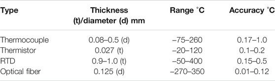
TABLE 4. Comparison of hard sensors.

3 Soft Sensors

Process or plant models designed to estimate various plant variables are known either as soft sensors, virtual sensors, inferential models, or estimators. Soft sensors are mostly used when it is difficult to use hard sensors in harsh environments or when hard sensors are not available. The estimation error to the respective reference value is considered as the accuracy of the soft sensors and standard deviations as precision when specified. The main steps for designing a soft sensor are data collection and filtering, variables, model structure selection, model identification (also known as parameterization) and model validation (Fortuna et al., 2007).

A general estimator would include a model that calculates the desired state, with the model value being updated by a value that corresponds to a correction term based on feedback measurements. The term estimation refers to the calculations of the state at current time based on the current or past measurements, while the term prediction refers to the estimation of a state at future time based on current or past measurements. A common estimation algorithm can be represented for state x as shown in Eq. 1, where $\widehat{x}$ is used for state estimates. Here, $x_k^{\text{m}}$, $y_k^{\text{m}}$ and y_k represent the model value of the state, the model value of measurements and the actual measurements, respectively at time k.

$\begin{array}{llll}\hfill {\widehat{x}}_k^{-}=& x_k^{\text{m}}\hfill & \hfill & apriori\text{\hspace{0.17em}state\hspace{0.17em}estimate}\hfill \\ \hfill e_k^{-}=& f\left(e_{k-1}^{+}\right)\hfill & \hfill & \text{estimation\hspace{0.17em}gain\hspace{0.17em}}\hfill \\ \hfill {\widehat{x}}_k^{+}=& {\widehat{x}}_k^{-}+e_k^{-}\left(y_k-y_k^{\text{m}}\right)\hfill & \hfill & aposteriori\text{\hspace{0.17em}state\hspace{0.17em}estimate}\hfill \\ \hfill e_k^{+}=& g\left(e_k^{-}\right)\hfill & \hfill & \text{estimation\hspace{0.17em}gain\hspace{0.17em}update}\hfill \end{array}(1)$

The first two are known as time updates where the latter are known as measurement updates or corrections. The calculation and update of estimation gain is the main difference among estimators as functions f and g are different for each estimator. The choice of the estimator depends on the system, the type of model and measurements.

The measurements of the soft sensor can be onboard measurements, such as the surface and ambient temperature, current, and voltage. Any observable battery model system can be used for this. The model can be a black box model or a mathematical model based on physics or a combination of these two. For linear models, a Kalman filter (KF) or a linear observer is the optimum estimator, while for nonlinear models other nonlinear estimators can be used.

The soft sensors that are reported in the literature are discussed based on the type of model that is used; a mathematical model-based or hybrid model-based. The mathematical model-based sensors are categorized based on bulk temperature estimation, distributed temperature estimation, and the type of thermal model of heat generation of the battery.

3.1 Mathematical Model-Based Estimators

Estimators that use physics-based mathematical models are discussed here which are mainly categorized in to local bulk temperature estimation and distributed temperature estimation.

3.1.1 Estimators of Bulk Internal Temperature

A simple model for any geometrical shape of the battery can be developed using the energy balance for the cell assuming constant heat capacity and a bulk internal temperature of the cell.

The definition of enthalpy (H = U + pv) can be used together with the first law of thermodynamics (ΔU = Q − W) as follows,

$\dot{H}=\dot{U}+\dot{\left(pv\right)}=\dot{Q}-\dot{W}+\dot{\left(pv\right)},(2)$

where H is the enthalpy, U is the internal energy, p is the pressure, v is the volume, Q is the heat added to the system, and W is the work done by the system on the surroundings. The work can be expressed as a combination of pressure-volume work and other work such as electrical, magnetic, or gravitational work. Using only the rate of pressure-volume work $(p\dot{v})$ and the rate of electrical work (IV) and neglecting other works, the expression 2 can be re-arranged as follows for a constant pressure system,

$\dot{H}=\dot{Q}-p\dot{v}-IV+p\dot{v}=\dot{Q}-IV,(3)$

where I is the current and V is the voltage of the electrical system.

The rate of enthalpy can be written for a multi-phase system with multiple species and of nonuniform composition, as follows (Thomas and Newman, 2003),

$\dot{H}=\int \sum _j\sum _i\frac{\partial c_{ij}{\bar{H}}_{ij}}{\partial t}\mathrm{d}v+\oint \sum _j\sum _i{c}_{ij}{\bar{H}}_{ij}u\mathrm{d}S,(4)$

where c_ij (x, y, z, t) is the concentration of specie i of phase j, and ${\bar{H}}_{ij}(c,p,T)$ is the partial molar enthalpy of specie i of phase j (Thomas and Newman, 2003). Here, x, y, z are the spatial position in Cartesian coordinates, and T is the temperature, u is the velocity of the boundary, and dS is a differential area of the surface of the system. The second term on the right-hand side of Eq. 4 is for the systems with changing volume. This term can be neglected by assuming that the change of the volume in LIBs is comparatively small. With the use of the Gibbs-Duhem equation, Eq. 4 can be expressed as follows (Thomas and Newman, 2003),

$\dot{H}=\int \sum _j\sum _i{\bar{H}}_{ij}\frac{\partial c_{ij}}{\partial t}\mathrm{d}v+\int \left(\rho \frac{\partial \tilde{H}}{\partial T}\frac{\partial T}{\partial t}+\rho \frac{\partial \tilde{H}}{\partial p}\frac{\partial p}{\partial t}\right)\mathrm{d}v,(5)$

where ρ is the bulk density and $\tilde{H}$ is the specific enthalpy of the system. Assuming that the cells are thermally thin (heat conduction in cell is faster than surface convection; Biot number is less than 0.1), and therefore, the temperature is considered uniform, the equation can be simplified as follows,

$\dot{H}=\dot{Q}-IV=\int \sum _j\sum _i{\bar{H}}_{ij}\frac{\partial c_{ij}}{\partial t}\mathrm{d}v+C_{\text{p}}\dot{T}.(6)$

Here, C_p is the specific heat capacity of the cell, and T is the internal bulk temperature of the cell. Defining a partial molar enthalpy evaluated at the volume-averaged concentration at any point in time as ${\bar{H}}_{ij}^{\text{a}}$, the enthalpy changes due to mixing and reaction can be separated into individual terms as follows for electrochemical reactions and chemical reactions,

$\dot{H}=\dot{Q}-IV=\int \sum _j\sum _i\left({\bar{H}}_{ij}-{\bar{H}}_{ij}^{\text{a}}\right)\frac{\partial c_{ij}}{\partial t}\mathrm{d}v+C_{\text{p}}\dot{T}+\sum _m\mathrm{\Delta }{H}_m^{\text{a}}{r}_m-\sum _n{I}_n{U}_n^{\text{a}}+\sum _n{I}_{n}T\frac{\partial U_n^{\text{a}}}{\partial t}.(7)$

Here, $\mathrm{\Delta }{H}_m^{\text{a}}$ is the enthalpy of reaction for chemical reaction m, which is evaluated at the volume-average composition in the cell, r_m is the rate of chemical reaction m, I_n is the amount of the total current passed through the electrochemical reaction n, and $U_n^{\text{a}}$ is the enthalpy potential of electrochemical reaction n, which is evaluated at the volume-average composition in the cell. Rearranging Eq. 7, the following expression can be obtained for the heat added to the system.

$\dot{Q}=C_{\text{p}}\dot{T}+\underset{\text{resistive\hspace{0.17em}heat}}{\underset{<unknownfont>︸</unknownfont>}{\left(IV-\sum _n{I}_n{U}_n^{\text{a}}\right)}}+\underset{\text{entropic\hspace{0.17em}heat}}{\underset{<unknownfont>︸</unknownfont>}{\sum _n{I}_{n}T\frac{\partial U_n^{\text{a}}}{\partial t}}}+\underset{\text{reaction\hspace{0.17em}heat}}{\underset{<unknownfont>︸</unknownfont>}{\sum _m\mathrm{\Delta }{H}_m^{\text{a}}{r}_m}}+\underset{\text{heat\hspace{0.17em}of\hspace{0.17em}mixing}}{\underset{<unknownfont>︸</unknownfont>}{\int \sum _j\sum _i\left({\bar{H}}_{ij}-{\bar{H}}_{ij}^{\text{a}}\right)\frac{\partial c_{ij}}{\partial t}\mathrm{d}v}}(8)$

The second term is the irreversible resistive heating, which occurs due to the deviation of the cell potential from its equilibrium potential by the resistance of the cell to the passage of current. The third term is the reversible entropic heat while the fourth term is the heat caused by the chemical reactions (Thomas and Newman, 2003). This is analogous to the heat generation terms commonly used in electrochemistry (see Figure 6A). Thomas and Newman (2003) have also shown how the model can be extended for localized temperature instead of cell averaged temperature, using a locally averaged concentration and more localized heat of mixing and enthalpy potential (e.g., across each electrode), and with the inclusion of the heat of mixing within each particle. As this is developed using Cartesian coordinates, the model applies to both prismatic and pouch cells; however, for cylindrical cells, the model needs to be converted to cylindrical coordinates and appropriate assumptions need to be made accordingly.

FIGURE 6

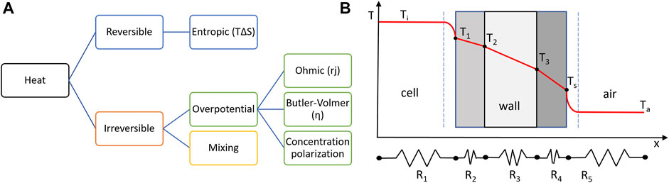
FIGURE 6. A common illustration of (A) heat generation categories in batteries, (B) the heat transfer mechanism from inside the cell to the surrounding environment.

This model can be expressed in a composite manner for the internal bulk temperature of the cell (T_i) as follows, expressing Q as the heat dissipated out of the system to the surroundings (−Q•_o) and the rest of the heat terms as the heat generated in the system (+Q_g),

$C_{\text{p}}{\dot{T}}_{\text{i}}=-{\dot{Q}}_{\text{o}}+{\dot{Q}}_{\text{g}}.(9)$

${\dot{Q}}_{\text{g}}=IV-\sum _n{I}_n{U}_n^{\text{a}}+\sum _n{I}_{n}T\frac{\partial U_n^{\text{a}}}{\partial t}+\sum _m\mathrm{\Delta }{H}_m^{\text{a}}{r}_m+\int \sum _j\sum _i\left({\bar{H}}_{ij}-{\bar{H}}_{ij}^{\text{a}}\right)\frac{\partial c_{ij}}{\partial t}\mathrm{d}v(10)$

Here, ${\dot{Q}}_{\text{o}}$ is considered as the net rate of heat transfer out of the cell and can be taken as a composite heat transfer system as follows, using all three forms of heat transfer, conduction, convection, and radiation as shown in Figure 6B. The heat transfer can be expressed in various ways using equivalent thermal resistances (Rs) in the cell, composite wall, or the outer air as follows, and with the use of various temperatures such as the surface temperature (T_s) and the outside air temperature (T_a),

${\dot{Q}}_{\text{o}}=\frac{T_{\text{i}}-T_1}{R_1}=\frac{T_1-T_2}{R_2}=\frac{T_2-T_3}{R_3}=\frac{T_3-T_{\text{s}}}{R_4}=\frac{\left(T_{\text{i}}-T_{\text{s}}\right)}{R_{\text{w}}}=\frac{T_{\text{s}}-T_{\text{a}}}{R_5}+\frac{\left(T_{\text{s}}^4-T_{\text{a}}^4\right)}{R_{\text{r}}}(11)$

Estimators With Ohmic Resistive Heating

Most of the thermal models in the literature are based on simplified versions of models with ohmic resistive heating. The simplest version is using only ohmic heating for heat generation in the cell together with simplified equivalent resistance for heat transfer. Slightly different variations of this simplest model are commonly used in battery modeling and also known as the lumped parameter thermal model, or conventional linear model. The main challenge of these models is the accurate calculation of the internal resistance of the cell.

Zhang et al. (2016) used the following model with a commonly used equivalent electric circuit model of a single resistor (R_c) and a first order resistor-capacitor (RC) circuit in series for capturing cell relaxation,

$\begin{array}{cc}\hfill C_{\text{p}}{\dot{T}}_{\text{i}}=& I{R}_{\text{c}}^2-k_1\left(T_{\text{i}}-T_{\text{s}}\right),\hfill \\ \hfill C_{{\text{p}}_2}{\dot{T}}_{\text{s}}=& k_1\left(T_{\text{i}}-T_{\text{s}}\right)-k_2\left(T_{\text{s}}-T_{\text{a}}\right),\hfill \end{array}(12)$

where R_c is the internal resistance of the cell, $C_{{\text{p}}_2}$ is the heat capacity of the cell container, and k₁, k₂ is the heat conduction coefficients for the cell and the outside air, respectively. This thermal model is coupled with the electric model for SOC, voltage, and overpotential. Test data is used for parameter identification of both the models using least square methods. The battery internal resistance R_c is calculated based on instantaneous voltage and load current jumps, and a relationship between the tested cell internal temperature and R_c is developed from the tests of a prismatic LFP battery. The R_c for the model is calculated by linear interpolation of this relationship. Based on these parameters, the cell temperature and the surface temperature are found. The internal cell temperature results are compared with experimental results and root mean squared error (RMSE) is reported as 0.37°C and the maximum error is 1.28°C. Similarly, the surface temperature of the cell is compared with experimental results and the RMSE is 0.36°C, while the maximum error is 1.43°C. These model results are shown in Figure 7A.

FIGURE 7

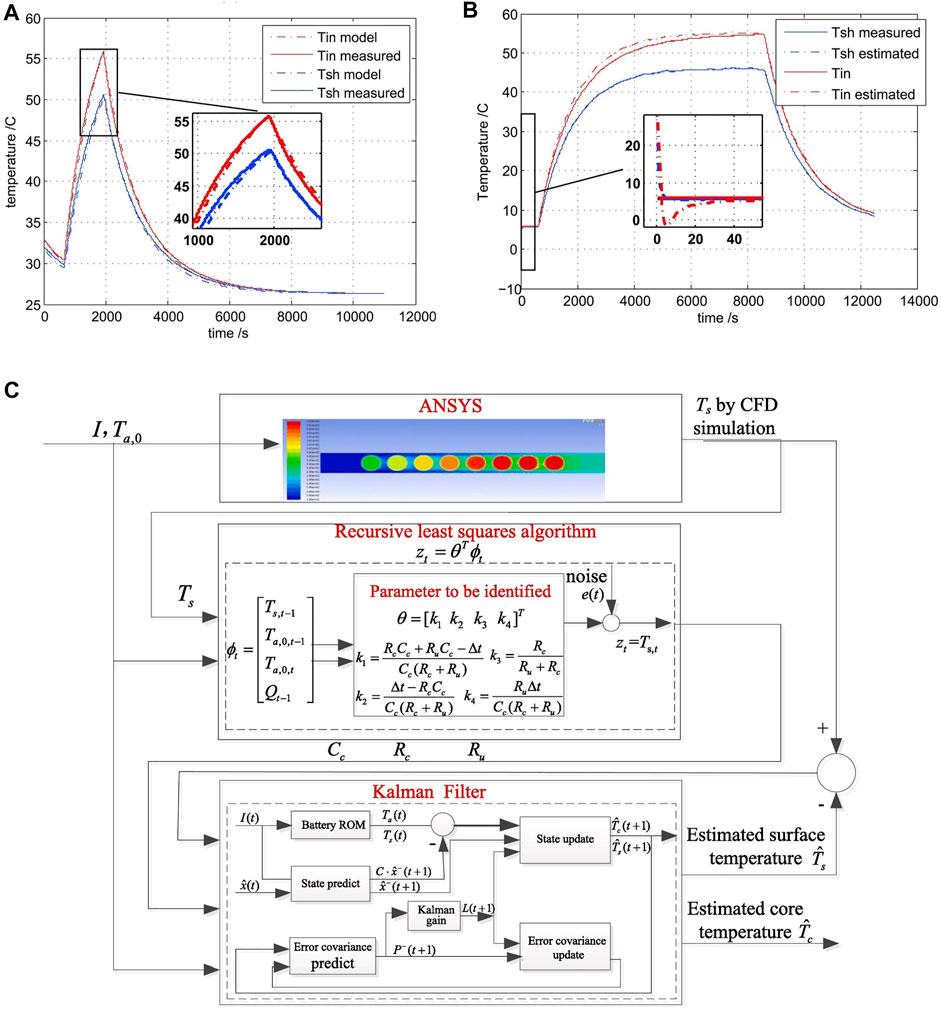
FIGURE 7. (A) Model results (EKF) at an ambient temperature of 26.3°C (Zhang et al., 2016; Panel 7B, p. 151) and (B) EKF estimation results at an ambient temperature of 5.5°C (Zhang et al., 2016; Panel 8A, p. 153). T_in: internal temperature, T_sh: surface temperature. (C) Structure of the parameter identification and temperature estimation method (Ma et al., 2020; Panel 14, p. 6). Reprinted from (Zhang et al., 2016), Copyright (2016); reprinted from (Ma et al., 2020), Copyright (2020) with permission from Elsevier.

The coupled model is then rearranged in the state-space form, and the states SOC, R_c, T_s, and T_i are estimated in real-time using an extended Kalman filter (EKF). The measurements used are the battery voltage, current, and surface temperature. The initial error in the internal temperature estimation has converged to zero in less than 60 s as shown in Figure 7B, and the RMSE is reported as 1.01°C. A slight deviation from the actual value of about 1°C during the temperature increase was observed, which could have been caused by the inaccuracies of the simplified model. Further, the estimation error of SOC is around 1.5%, which is a reasonable accuracy. However, the simplified circuit model was not able to capture the full relaxation dynamics, and the effects of temperature and hysteresis on battery OCV were not considered in the model, which could give larger estimation errors for SOC estimations (Zhang et al., 2016).

The same model (Eq. 12) for a set of cylindrical cells was applied by Ma et al. (2020) with an additional equation for the outside air temperature of each cell as follows,

$C_{{\text{p}}_3}{\dot{T}}_{\text{a}}=\frac{\left(T_{\text{s}}-T_{\text{a}}\right)}{R_5}+{\dot{m}}_{\text{a}}{C}_{{\text{p}}_{\text{a}}}\left(T_{\text{a,\hspace{0.17em}i}-1}-T_{\text{a,\hspace{0.17em}i}}\right),(13)$

where $C_{{\text{p}}_3}$ is the heat capacity of the air, ${\dot{m}}_{\text{a}}$ is the mass flow rate of air between the cells, $C_{{\text{p}}_{\text{a}}}$ is the specific heat capacity of air, and i is the cell number in a row. T_i, T_s and T_a were taken as the states, the resistive heat and the air temperature of the previous cell (T_{a, i-1}) were inputs in the linear system, while the T_s was the measurement. From the tests on a single cell, a second order polynomial was fitted for the internal resistance of the cell, using the average temperature of T_s and T_i. For the rest of the parameters, off-line parameterization with recursive least squares was conducted for a single cell. The necessary temperature data for the parameterization was obtained from CFD simulation results. The model validation was done using similar CFD results for different air velocities in between the cells, the model errors for the surface temperature of cells have a maximum value of 0.6 K at a 3 m/s air velocity, and 0.5 K at a 0.1 m/s air velocity (Ma et al., 2020).

The validated model is then used with a KF to estimate the internal temperature based on the T_s measurements of the CFD results (Figure 7C). The estimation errors for the internal temperature of cells have a maximum value of 0.6 K at a 3 m/s air velocity, and 0.8 K at a 0.1 m/s air velocity (Ma et al., 2020). However, as the CFD simulation results are considered as the measurements for the estimator, the generated noise may not represent the real conditions, which could increase the estimation error compared to the reported values for real measurements.

The discussed models considered only the conductive and convective heat dissipation from the cell. Sun et al. (2020) extended the model for radiation while allowing the estimators to operate in the presence of sensor bias. For the thermal model the radiation heat term $(T_{\text{s}}^4-T_{\text{a}}^4)/R_{\text{r}}$ is added to the surface temperature in Eq. 12 as follows,

$C_{{\text{p}}_2}{\dot{T}}_{\text{s}}=\frac{\left(T_{\text{i}}-T_{\text{s}}\right)}{R_{\text{w}}}-\frac{\left(T_{\text{s}}-T_{\text{a}}\right)}{R_5}-\frac{T_{\text{s}}^4-T_{\text{a}}^4}{R_{\text{r}}}.(14)$

The state-space system was developed using the two temperatures as the states, squared current as input, and T_s as the measurement. A thermocouple is inserted into a cylindrical cell and T_s and T_i were measured in tests together with the other measurements, and these data are used for the model parameter identification. The optimum model parameters were obtained by using the non-dominated sorting genetic algorithm II, and it is shown by the root-mean-squares of the residuals of the temperatures, that the radiation term has added considerable accuracy in T_s calculations and a slight improvement in T_i calculation.

The estimations were done using an extended state observer based approach, as it can account for both nonlinear uncertain dynamics and the variation of uncertainties (Guo and Zhao, 2011; Xue et al., 2015). Sun et al. (2020) have introduced the sensor bias as an additional state and augmented with the rest of the states with an additive noise term. If a normal nonlinear state-space system in its discrete form can be expressed as follows,

$\begin{array}{cc}\hfill x_{k+1}=& f\left(x_k,u_k\right)+w_k,\text{and}\hfill \\ \hfill y_k=& g\left(x_k,u_k\right)+v_k,\hfill \end{array}(15)$

then the extended state observer system is expressed with the extended states x′ such that $x_k^{\prime }={[x_k^{\top }{b}_k]}^{\top }$, with the sensor bias (b_k) as the augmented state. The augmented state is updated as a piecewise constant state as f (3) = b_k, the output equation for the surface temperature is changed to $g(x_k^{\prime },u_k)+b_k$, and the input is updated as u_k − b_k for the bias correction (Sun et al., 2020). An unscented Kalman filter (UKF) algorithm of uniformly distributed sigma points is followed for this extended system and named as an extended unscented Kalman filter (EUKF) by the authors.

The results of the EUKF are compared with the UKF for online test results for a set of biased sensor measurements in the current, and the surface temperature, separately. In both the cases (as shown in Figure 8), the EUKF was capable to estimate the temperatures without the bias unlike the UKF, and the sensor bias estimation error convergence from the initial error has taken a considerable time, approximately 500–1,000 s. When there is bias in the input measurements, then the UKF gave biased estimations in both the internal and surface temperatures as expected. When there is bias on surface temperature measurement (no bias in inputs) the UKF gave correct surface temperature estimation. However, the internal temperature estimations were biased. This showed that both the UKF and EUKF are good for internal temperature estimation in general, as the sensor bias is affecting all types of estimators that are discussed here and have to be accounted for separately. In general, the addition of the radiation term in the heat transfer has improved the estimations considerably, compared to the estimation without the radiation term.

FIGURE 8

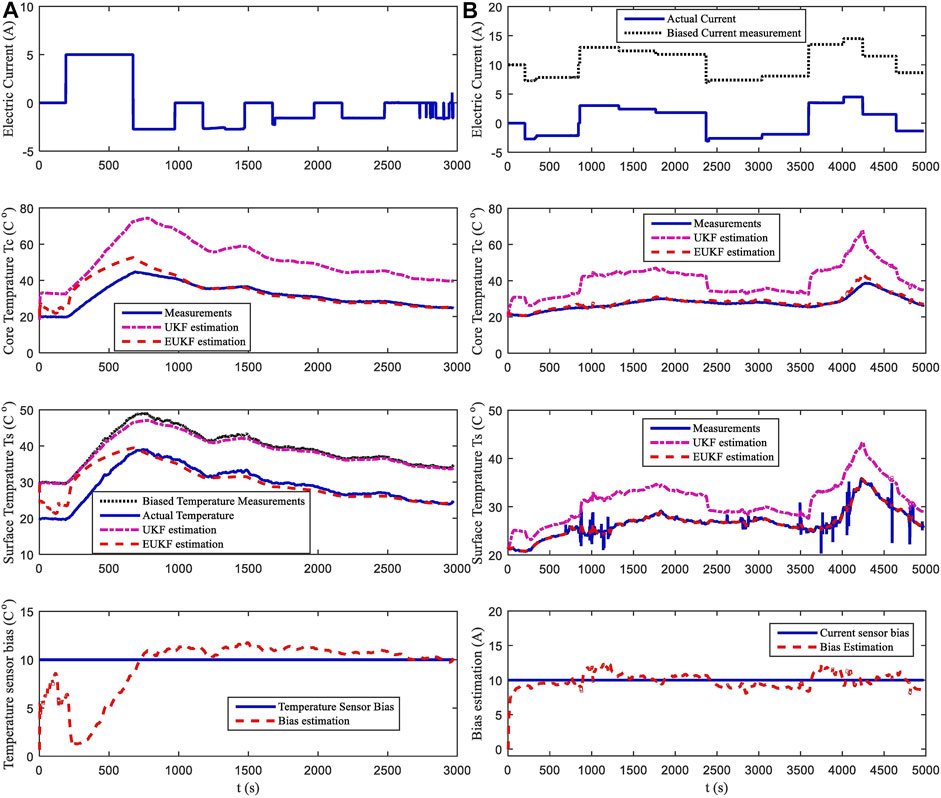
FIGURE 8. Online estimation results for both UKF and EUKF during charging and discharging tests. (A) with a 10°C sensor bias in the surface temperature measurement (Sun et al., 2020; Panel 13, p. 11). (B) with a 10 A sensor bias in the current measurement with additional noise (Sun et al., 2020; Panel 14, p. 12). Reprinted from (Sun et al., 2020), Copyright (2020) with permission from Elsevier.

The same first-order RC circuit model with ohmic heat is used for internal temperature estimation by Zhu C. et al. (2020), with a self-heater for automotive batteries that operate in cold climates. Since there is a self-heating unit on board with the battery pack, the current measurements are not available for this application during heating, unlike the other estimators that were discussed above. The model is the same as shown in Eq. 12, with two additional inputs (surface temperature) from the adjacent cells. The current and the internal resistance are inaccurately estimated at the beginning, and these estimates are considered as one of the inputs instead of the real value of I²R_c. The disturbance caused by these inaccurate estimations is considered as a state (as the root mean squared value of the disturbance; $d=I^2{R}_{\text{c}}-{\widehat{I}}^2{\widehat{R}}_{\text{c}}$) together with the internal and surface temperatures. A linear observer is designed for this augmented linear system (an ESO), and the initial error that occurs due to inaccurate internal resistance and current value converges to zero, as the observer ensures that the disturbance diminishes over time. This is the same underlying basic principle that was used by Sun et al. (2020) to eliminate the sensor bias in the inputs and measurements. Therefore, any suitable KF variant could have been used in this application as well, although the authors claim that a KF is not usable due to the lack of current measurements. The use of ESO in the presence of high noise can be problematic due to its deterministic nature as opposed to the stochastic nature in KFs. Similarly, the use of KF could be problematic in an application of a high number of cells in a row of a pack, as the inversion of matrices with larger size could be computationally heavy as opposed to the direct calculation of observer gain in ESOs.

The ESO is tested online with six 2,500 mAh, 18 ,650 LMO cells where the surface temperatures were monitored using K-type thermocouples. Urban dynamometer driving schedule cycles were performed and the data were used for parameter identification of the model. For the reference internal temperature values, EIS-based internal temperature estimations were used instead of an insertion of a thermal sensor into the cells. The test results showed that the internal temperature estimates are accurate (estimation error was less than 0.6°C) and converge fast when the mismatch of internal resistance is comparatively low. When the mismatch is higher (15:1,500 mΩ) the internal temperature has an offset throughout the heating period, until it converges again when the measurements are available. During this offset, the estimation error is less than 1.2°C, which suggests that the ESO compensates well enough even for high model parameter mismatches.

Zhang et al. (2020) also used the same thermal model to inversely estimate the heat generation inside the cell, while Debert et al. (2013) used the model as a linear parameter varying model and estimated the temperature using a polytopic observer. The model expands to three temperature equations, where the surface temperature is considered as the cell surface temperature and an additional cell casing temperature is calculated outside the cell surface. The internal resistance is considered as a time-variant parameter $(\dot{R}=0)$ and estimated together with the other states. The output internal cell temperature is measured using a thermocouple, and the input is considered as the ambient air temperature, while the estimated states are the internal temperature, cell surface temperature (measured by a thermistor), cell casing temperature (measured by a thermocouple), and the internal resistance. A typical electric vehicle drive test was carried out on a four-cell module to identify the thermal resistances using a Nelder-Mead simplex optimization algorithm. The model is then validated using test data, where the RMSE is 1.6°C for the internal temperature.

A linear observer is designed for this linear system, and the observer validation results are shown in Figure 9A, where the RMSE for internal cell temperature is reduced down to 0.38°C from model to estimation. However, the system is reported to be not observable at near-zero currents; therefore, for currents less than 0.5 A (which is considered as a maximum sensor error) the system does not estimate and only the open-loop model calculations are performed. This could have been improved by a lesser observable system during this time frame by estimating only the temperatures and considering a constant internal resistance.

FIGURE 9

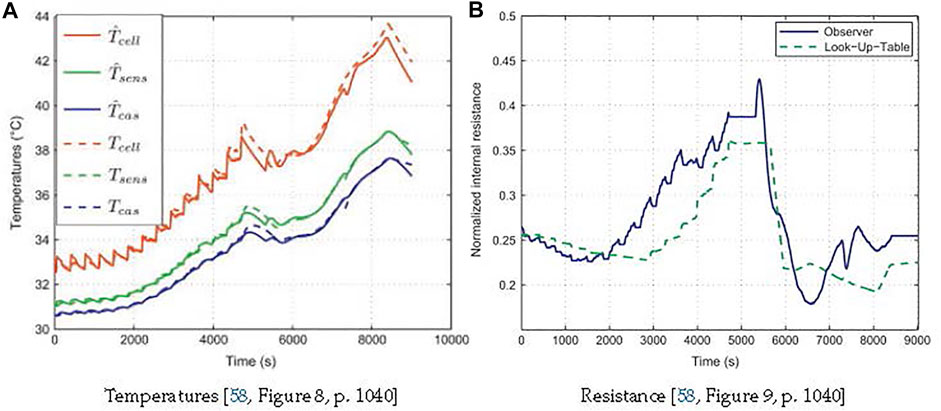
FIGURE 9. The estimation results, (A) temperatures, (B) internal resistance against the actual values. Internal temperature is denoted as T_cell, surface temperature is denoted as T_sens and the casing temperature is denoted as T_cas. Reprinted from (Debert et al. (2013)), Copyright (2013) with permission from Elsevier.

Further, the estimated R_c closely followed the lookup table values as shown in Figure 9B, which are based on different temperature and SOC values. As is evident from all the models, the model parameter identification is of high importance in these model-based estimators. The R_c is the most important parameter among these. Therefore, the ability to simultaneously estimate the R_c is highly valuable in an estimator, such that the estimator can be easily used in various dynamic conditions without any major offline parameterizations.

Estimators With Resistive and Entropic Heating

The heat generation term with partial resistive heat that was discussed earlier has been modified by adding the entropic heat by Xie et al. (2020). They used a 1-D thermal model with three nodes along the length of the core of a cylindrical cell from the middle to the top. The system of equations was reduced to three ordinary differential equations (ODEs) with the finite difference method. To estimate the R_c, they have used the model by Ding and Chen (2005) which expresses the terminal voltage in terms of overall current and the dynamic internal resistance. The unknown parameters and states of this model are found by recursive extended least-squares algorithm, where the R_c including ohmic and polarization resistances is estimated together with the noise of the first-order RC circuit. This model is then further extended into linear state-space form and used with KF to estimate the SOC. Another KF is jointly used with the thermal model to estimate the three temperatures. The remaining geometrical parameters were found by various approximations and tests. Several experimental data sets were used for the validation of the estimators, and it was shown that the estimations are accurate and also shows that the initial error can be converged to zero approximately within 1,000 s. Since the T_is are not measured in the tests, a CFD simulation has been carried out to assess the estimation accuracy of the KFs. The RMSE values of the two T_i estimates compared to the CFD values are 0.2891 and 0.2767°C (first node at the middle of the cell and the second closer to the top), where the T_s estimate has a RMSE value of 0.04°C. Although these values are comparatively low, it is difficult to determine whether this accuracy is due to the addition of the entropic heat to the thermal model, or due to the dynamic estimation of the internal resistance. However, the addition of both have considerably increased the accuracy of the temperature estimations. The estimation accuracy could be reduced when it is used with real measurements, rather than using CFD measurements that contain no noise and disturbances.

On the other hand, Xiao (2015) used the complete resistive heat term and the entropic heat term in Eq. 10 for the heat generation of the cell model. The cell has been divided into two layers (core and surface) and then each layer is divided into several nodes, and for each node the thermal model is considered. They have plotted the resistive heat and the total heat with inclusion on entropic heat for a cell for 1C rate, and from 0 to 2,500 s the resistive heat is higher than the total heat by about 3 W and after 2,500 s total heat dominates with an increasing margin up to about 8 W. This shows that even at 1C rate the heat generation can be improved by the addition of entropic heat. Although this has given a slight improvement in the temperature calculation with entropic heat, this is not a significant improvement compared to the temperature. Further, what caused the sudden change at 2,500 s for the heat generation is not stated in the study. The state-space system developed based on the model contains two states, the voltages of the core and surface layer, and the heat generation at the core layer as the input. The model parameters were obtained from the battery dimensions, material properties and experimentally measured heat transfer coefficient. The calculations using these parameters have shown that the maximum temperature calculation error for different test conditions were 0.4–0.9°C. Then the parameters were tuned using a prediction error minimization method, and the calculations with tuned and initial parameters were compared together. It can be seen that the model parameterization has a considerably larger effect than the addition of entropic heat, where the parameterization has shown a significant reduction of error, where the maximum error with initial parameters was 0.64–1.1°C while the maximum error with tuned parameters was 0.3–0.6°C for various nodes. Then the tuned model was used with a KF for estimating the temperature. The observability conditions revealed that the system is observable only when the number of measurements is the minimum number of surface temperature measurements that are obtained from the cell (12 in this study). The optimum locations for the temperature sensors (type J thermocouples) were found by testing various locations and determining the mean squared error of real and estimated temperatures. Once the locations were found, the temperature estimations were carried out. The KF was started with large initial errors (10°C) but quickly converged to zero within about 15 s. The estimation error of the KF is stated as 0.1°C (possibly the maximum error) and the time duration for the estimation is mentioned as less than 2 s.

Rath et al. (2020) used the same heat generation model for a battery module of 36 cells with top and bottom cooling plates. Therefore, the equation of the surface temperature of the cell contains the heat transfer with adjacent cells, with the top and bottom plates, and with the ambient air. Similarly, the model contains two additional equations for the top and bottom plates, which are dominated by convection cooling. These four equations for a common cell can be rearranged into a linear state-space system. The thermal capacity of a single cell was found using an accelerating rate calorimeter. The remaining parameters were identified using various test results. As the tests did not include the internal temperature measurements, a 3-D finite element model was used to generate the necessary data for resistance values. A KF-based estimator was applied to match the model and test results of worldwide harmonized light vehicle test drives. Since only the surface temperature measurements are available, the estimations are only compared with surface temperatures, where the maximum RMSE was 0.6°C both at normal operation and at sensor failure conditions, while the error is 0.75°C during sensor malfunction. It is reported that in all operating conditions and at every ambient condition that is tested, the RMSE remains well below 1.5°C. However, as only the surface temperatures are available, it is difficult to get an assessment on whether the inclusion of entropic heat has improved the estimations. Furthermore, it is also shown that the entropic heating can be insignificant to Ohmic heating at higher charging rates (4–12C) and can be significant as much as Ohmic heating at lower charging or discharging rates (1–2C) (Burheim et al., 2014). This could also change based on the cathode chemistry of the cell (Burheim et al., 2014).

3.1.2 Estimators of Distributed Internal Temperature

Richardson et al. (2014) used a steady-state thermal model in cylindrical coordinates for a cylindrical cell coupled with a thermal impedance model so that the internal temperature can be estimated with the use of an EIS system. The steady-state thermal model gives the temperature distribution of the cell with respect to the radius (r) as follows,

$\begin{array}{cc}\hfill T\left(r\right)=& T_{\text{s}}+a{r}_{\text{o}}^2\left(1-\frac{r^2}{r_{\text{o}}^2}\right)\left[1-\frac{\ln \left(r_{\text{o}}/r\right)}{\ln \left(r_{\text{o}}/r_{\text{i}}\right)}\right]-\left(T_{\text{s}}-T_{\text{i}}\right)\frac{\ln \left(r_{\text{o}}/r\right)}{\ln \left(r_{\text{o}}/r_{\text{i}}\right)},\hfill \\ \hfill \text{with,}a≔& \frac{T_{\text{i}}-T_{\text{s}}}{r_{\text{o}}^2-2r_{\text{i}}^2\ln \left(r_{\text{o}}/r_{\text{i}}\right)+1},\hfill \end{array}(16)$

where r_i and r_o the radius of the center core, and the outer surface, respectively. This expression is then used with the measured admittance of the cell to get an expression for the maximum temperature of the distribution, which is at the core (r_i) and interpreted as the internal cell temperature (T_i). Although this does not include an estimation algorithm, it directly calculates the temperature based on online EIS and surface temperature measurements with a maximum error of 0.9°C. This study shows that the temperature distribution is important as the maximum temperature of the distribution is the best fit with the real measurements at the core, while a uniform distribution would always underestimate the temperature by a mean error value of 2.6°C.

However, as this is a direct calculation without a feedback correction term, this error in a uniform distribution can be reduced further. Similarly, the use of maximum temperature from the distribution would reduce the error even more. Kim et al. (2013) have used a similar method with a KF, where they have used the 1-D unsteady heat conduction equation for a cylinder as the thermal model as follows,

$\rho {\mathit{C}}_{\text{p}}\frac{\partial T\left(r,t\right)}{\partial t}=k_3\frac{{\partial }^{2}T\left(r,t\right)}{\partial r^2}+\frac{k_3}{r}\frac{\partial T\left(r,t\right)}{\partial r}+\frac{{\dot{Q}}_{\text{g}}}{V_{\text{c}}},(17)$

with the boundary conditions:

$\begin{array}{cc}\hfill k_3{\left.\frac{\partial T\left(r,t\right)}{\partial r}\right|}_{r=0}=& 0\hfill \\ \hfill {\left.\frac{\partial T\left(r,t\right)}{\partial r}\right|}_{r=r_{\text{o}}}=& -\frac{h}{k_3}\left(T\left(r_{\text{o}},t\right)-T_{\text{a}}\right)\hfill \end{array}(18)$

where V_c is the volume of the cell, k₃ is the thermal conductivity, and h is the convective heat transfer coefficient. The solution to the unsteady thermal model T (r, t) is approximated by a fourth-degree polynomial of the parameter (r/r_o) where the polynomial coefficients are considered time-dependent. Using this temperature expression, the two states (T_V, T_G) of the system are derived by integrating over the radius, where T_V is the volume averaged temperature and T_G is the temperature gradient along the radius. This allowed the polynomial coefficients of the temperature distribution T (r, t) to be expressed in terms of T_V, T_G, T_s and r_o. A similar expression for the surface temperature T_s (k, h, T_V, T_G, T_a) was developed using the boundary condition of the unsteady model where convective heat transfer happens at the outer surface of the cell taking h as the convective heat transfer coefficient.

The system in continuous form is then arranged for the two states using the heat generation and air temperature as inputs, with the two additional equations for T_i and T_s as follows,

$\begin{array}{cc}\hfill {\dot{T}}_{\text{V}}=& \frac{-48\alpha h}{b{r}_{\text{o}}}{T}_{\text{V}}-\frac{15\alpha h}{b}{T}_{\text{G}}+\frac{\alpha }{kV}{\dot{Q}}_{\text{g}}+\frac{48\alpha h}{b{r}_{\text{o}}}{T}_{\text{a}},\hfill \\ \hfill {\dot{T}}_{\text{G}}=& \frac{-320\alpha h}{b{r}_{\text{o}}^2}{T}_{\text{V}}-\frac{120\alpha \left(4k+r_{\text{o}}h\right)}{b{r}_{\text{o}}^2}{T}_{\text{G}}+\frac{320\alpha h}{b{r}_{\text{o}}^2}{T}_{\text{a}},\hfill \\ \hfill T_{\text{i}}=& \frac{24k-3r_{\text{o}}h}{b}{T}_{\text{V}}-\frac{15r_{\text{o}}\left(8k+r_{\text{o}}h\right)}{8b}{T}_{\text{G}}+\frac{4r_{\text{o}}h}{b}{T}_{\text{a}},\hfill \\ \hfill T_{\text{s}}=& \frac{24k}{b}{T}_{\text{V}}-\frac{15r_{\text{o}}k}{2b}{T}_{\text{G}}+\frac{r_{\text{o}}h}{b}{T}_{\text{a}},\hfill \\ \hfill \text{with,}b≔& 24k+r_{\text{o}}h,\text{and}{\dot{Q}}_{\text{g}}=IV-I{U}_{\text{OCV}},\hfill \end{array}(19)$

where α is the thermal diffusivity and U_OCV is the open-circuit voltage which is considered as the bulk enthalpy overpotential of all the reactions. The model parameter identification was carried out by minimizing the error between model and test values from ‘urban-assault driving cycle’ experiments. The same states and inputs are rearranged in state-space form together with the measurement equation for the state estimation using a KF with the test results of an escort convoy driving cycle. The RMSE value of the internal temperature estimations is reported as 0.2°C.

Further, Kim et al. (2014) have extended this study to establish that the heat transfer coefficient h has the highest sensitivity on the model; therefore, h is estimated separately as a parameter together with the states. For this parameter estimation, the parameter is included in the system as a piecewise constant with additive white noise (h_k+1 = h_k + z_k). The system was then tested by dual extended Kalman filter (DEKF), where a separate parameter filter goes through the same update process but with the updated a posteriori state ${\widehat{x}}_k$ and the a priori parameter state ${\widehat{h}}_{k-1}$ (Wan and Nelson, 2001). The temperature measurements were taken using type-T thermocouples and tests were done for “escort convoy driving cycle” under various cooling conditions. The KF showed accurate results as long as the correct h was given, while the DEKF was able to compensate for the error in h though it takes a considerable time to converge (400 s), and both have the same RMSE value of 0.26°C. When the cooling conditions suddenly changed, the RMSE of DEKF increases (0.39°C) as it takes a longer time to accurately estimate the h. When the initial h was given to the KF as twice the actual value, it overestimated the temperature about 0.5°C and the RMSE value was increased up to 1.18°C, while the DEKF estimated correctly with an RMSE of 0.31°C. Furthermore, the parameter estimation error converged to zero within about 500 s.

Richardson and Howey (2015) used the same model, estimation, and the method with EIS measurement system and compared with the T_s measurement system. Therefore their model has an additional impedance measurement, which is expressed as a function of the states (T_V, T_G) and the air temperature T_a. Then in the state-space model, both the measurements; the impedance and T_s, are taken as the measurement equation, one at a time. In addition to the EKF, and DEKF, a dual Kalman filter (DKF) was used. The results are similar to the results of Kim et al. (2014), where the EKF with impedance measurement overestimated the T_i and underestimated the T_s by approximately 2°C, when the heat transfer coefficient was twice the true value. The DEKF estimation had RMSE values of 0.47 and 0.42°C after the error convergence, for T_i and T_s, respectively. However, the error convergence took a longer time (approximately 1,200 s) to come to zero from the high mismatch that was introduced initially. Similarly, from the KF and DKF results when T_s was the measurement, the KF had an offset of 3°C (maximum) with the actual values, and the DKF has shown superior results to the DEKF according to the RMSE values of 0.16 and 0.14°C after the error convergence, for T_i and T_s, respectively. Further, the convergence of the DKF is comparatively quicker than with the DEKF. Both the studies show again that the parameter identification is crucial for the estimation, and the parallel estimation of critical parameters together with the maximum temperature provides better estimations even with a simplified lumped thermal model.

Richardson et al. (2016b) further modified the model into 2-D by including the longitudinal direction for the thermal model and improved the computational time by solving it using the spectral Galerkin method with Chebyshev approximation. The model was tested for different cooling methods and validated against commercial finite element method-based solutions. Additional measurements were taken by three thermocouples on the cell surface along the length. This model is then used with an EKF with impedance measurements and KF with surface temperature measurements from tests done on an Artemis driving cycle with cell cooling (Richardson et al., 2016a). Two configurations were tested with cooling for a fully insulated cell and without cooling for a normal cell, where the measurements were taken using three different current excitation profiles, named HEV-I, HEV-II, and HEV-III, where these cycles were generated by looping over different portions of the Artemis HEV drive cycle. HEV-I was used for parametrization and the rest were used for estimation (Figure 10).

FIGURE 10

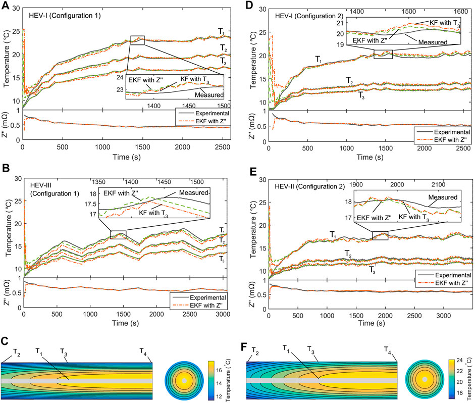
FIGURE 10. Estimation results of EKF with impedance and KF with surface temperature measurement. (A) HEV-I test with cooling (B) HEV-III test with cooling (C) temperature distribution modeled at the end of the HEV-I cycle (D) HEV-I test with no cooling (E) HEV-II test with no cooling (F) temperature distribution modeled at the end of the HEV-II cycle (Richardson et al., 2016a; Panel 7, p.733). (CC BY-NC-ND 4.0).

The estimation results follow the actual values in general, except with the HEV-III test results where the temperature was considerably underestimated. The authors suspected that this may be due to the simplified thermal model which only has ohmic heating, as the underestimates dominated during periods with very low or zero applied currents. This suggests that the cell testing with various drive cycles is important to test the estimators in all possible conditions and more complete thermal models would increase the estimation accuracy, although this might increase the computational time. The RMSE values are quite similar between the configurations and driving cycles for each method, where the EKF with impedance has 0.2–0.7°C and the KF with temperature measurement has 0.1–0.4°C RMSE values. This suggests that the T_s measurement is more reliable for T_i estimations than the EIS method, possibly due to the higher accuracy of the used thermocouples sensors.

Wang and Li (2017) converted Eq. 17 into 2-D with the inclusion of longitudinal direction. A Karhunen-Loeve transformation method is used to approximate the model during the model order reduction to get a set of ODEs. Two different analytical expressions were developed as solutions to these ODEs for known cooling conditions, and unknown cooling conditions, where the h is adapted. Available heat generation data is used on a three-layer feed-forward neural network model to find out the relationship of heat generation in terms of the current, voltage, and mean temperature. The model parameters were identified using the Nelder–Mead simplex optimization method on a set of urban dynamometer driving schedule test data. The state-space form of the estimation system contains the time coefficients of each approximated basis function as states, the air temperature, and the generated heat expression from the neural networks model, together with the surface temperature as output. A DKF is used to jointly estimate both the states and the parameter h. The results showed higher accuracy compared to the other 2-D model based estimators discussed here, where the spatial normalized absolute error is between ±0.2°C and the RMSE over the spatiotemporal domain is 0.0946°C. This may be due to the dual effect of the model order reduction technique and the better thermal model approximation by the data-driven method where it has given a better accuracy within the tested drive range. However, one major drawback of the method is that the need of sufficient training of the model before estimation. Furthermore, it is stated that the trained model has not considered any battery aging problems. Therefore, sufficient training over all possible data ranges is needed in these types of models. However, this has several advantages as well. It is shown that the solution technique is more computationally efficient than the numerical methods, which allows the model to be faster in estimations. It is also shown that the temperature differences between the 2-D model and the 1-D model (where a bulk temperature is assumed instead of local temperatures) can reach up to 8°C over time for the same cell conditions.

A similar 2-D model was developed by Hu et al. (2021) for a pouch cell for estimation and control. Here, the 2-D transient heat conduction equation was written in Cartesian coordinates for width and length directions of the pouch cell, and then transformed in to unit spectral domain such that the orthogonal functions can be easily approximated. Then the model is reduced to ODEs by using the Galerkin method with Chebyshev polynomial approximations. The equivalent ohmic resistance was taken to be a combination of cell resistance in series with the resistance from the two tabs. The tabs are considered as separate lumped models, where the heat generation of tabs are considered to be only from I²R and the heat flow between tabs and cell body are considered only to be through convection. The Chebyshev Galerkin approximated model is used for the cell body with discretized elements. Therefore, for each element, the total heat generation is taken to be resistive and entropic heat where the resistive heat generation is taken to be from the ohmic and polarization resistances of the respective element. Seven T-type thermocouples were placed on the surface of a 20 Ah battery and 2 thermocouples were placed in the tabs, and the cell was tested for various conditions to obtain the test data. The particle swarm optimization method is used for parameterization. Data of 1C constant current excitation profiles at seven temperatures were used for parameterization of the lumped models for the two tabs. A hybrid pulse power characterization test was used to parameterize the 2-D cell body model. These parameters were used to calculate the heat generation and then compared with the values calculated by voltage difference method and overpotential method, where the parameterized method was the highest due to high valued resistances obtained. All the models were then validated where each temperature is calculated and then compared with the sensor values. The RMSEs were in the range of 0.006–0.277°C for different data sets. Although this method has not calculated nor estimated T_i, the fidelity and the short computational time it takes to solve shows that this can be used for T_i estimation of pouch cells.

3.2 Hybrid Model-Based Estimators

Similar to physics model-based estimators, we can use data-driven approaches for estimation. Although fully data-driven temperature estimation studies are not yet done, there exists a few that estimates SOC and other states in BMS (Li et al., 2019). However, there are also data-based methods that are combined with physics-based models and estimators. These are commonly called hybrid method-based estimators. Most of these BMS estimators use neural networks (NN), support vector machines, fuzzy logics and deep learning methods for various state estimations (How et al., 2019). These hybrid methods have been mainly used for various BMS thermal management related estimations (Liu K. et al., 2018; Zhang et al., 2019). These methods can also be adopted for T_i estimations of the cell.

There are a few hybrid method-based estimators for T_i estimation of the battery. One example is where Mehne and Nowak (2018) used a stochastic physics-based model for a LFP battery to estimate the temperature as a probability density function (PDF) by running Monte-Carlo simulations. The stochastic physics-based model is a coupled pseudo-2D electrochemical and thermal model of a cylindrical cell (Mehne and Nowak, 2017). The thermal model contains both convection and radiation from cell to the surroundings. For the probabilistic temperature determinations, an error model (a time-dependent stochastic multiplier included in the rate of heat generation) is added to this model as a stochastic extension. The model parameters need to be pre-calibrated and the prior PDF of the T_i can then be found using a summation of Dirac delta functions by running a certain number of realizations of the stochastic model ensemble. The uncertainty of this prior PDF is calculated by the variance and similarly the posterior variance is found based on a linear additive measurement model with Gaussian measurement noise. The procedure is similar to a particle filter with a single measurement update and the data worth of the measurements is done using the preposterior analysis. Various testing scenarios have been carried out for the performance testing of the estimator including uncertain future discharge conditions, and uncertain SOC for two different cases, where the discharge current is modeled either using a white noise model or an auto-regressive process. Predictions of T_i based on the two cases showed that the auto-regressive process has low prediction error than the white noise model, where the RMSE is ±0.18°C and ±0.3°C, respectively (for ± 3σ level of standard error). This study shows that when the T_s sensor provides inaccurate data, the discharge current measurement with auro-regressive modeling can improve the T_i predictions using this stochastic model. Although this can be used for predictions, it is not practical to use this as an online application for a shorter sampling time (less than 90 s), due to the high number of Monte-Carlo simulations that are needed to be run within the sampling time.

Similarly, Liu et al. (2016) used a hybrid estimator where they jointly estimated the temperature using both a linear NN model and an EKF. They have used current, voltage and surface temperature measurements as inputs to the linear NN to capture the dynamics where the model output is the internal temperature. A fast-forward, fast recursive algorithm is used to find the NN structure and for the parameterization, such that optimum inputs are selected, computational efficiency is improved and redundancy is minimized. The lumped battery thermal model with partial resistive heat (Eq. 12) based EKF is then used to estimate T_i based on the output of NN and the T_s measurements. This allows the EKF to filter out the noise and the outliers in the NN so that the total estimation error is reduced. The estimation error for different temperature ranges are stated, where the RMSE for NN model is 0.179–0.233°C and for both EKF and NN is 0.081–0.129°C. This shows that the addition of EKF has reduced the estimation error, however the EKF mainly acts as a filter to reduce noise rather than acting as an estimator. The reason is that the authors have used the EKF in a way that it relies on the NN output as a measurement, but the model contains a linear interpolation of the mathematical relationship for battery internal resistance which is obtained from the test results. Usually the EKF alone can achieve similar results, and the NN has not improved EKF performance. A similar performance could also be obtained from attaching a filter to the NN model and with less computational resources.

The inability to react to unpredicted outliers, the requirement of large amounts of data for training and the less global applicability of these models are some of the disadvantages of data-driven models. However, some of these can be avoided by using them together with physics-based methods as shown from the above examples.

3.3 Potential of Development of Soft Sensors

Simplified thermal models like the lumped thermal models or other cell level models considering homogenized properties, allow us to estimate an average cell temperature but prohibit localized hotspot prediction. More detailed models allow for hotspot prediction and better understanding of electrochemical processes, but depending on the model fidelity, computing requirements vary. If the computational cost is too high it becomes difficult to use those models in an online system and the trade-off between accuracy and applicability has to be considered.

Many studies utilize the coupling of an electrochemical and thermal model that incorporate heterogeneity at the microscopic length scale (Yan et al., 2013; Shirazi et al., 2015; Zhoujian et al., 2018). Multi-physics models allow to analyze and predict electrochemical reactions and transport processes and the associated heat generation spatially resolved.

Spitthoff et al. (2021) developed a model considering the electrode layer and surface layer distinctly including the coupling of heat, mass and charge transport. Instead of including the reversible entropic heating by using the entropy change over the full cell, the reversible heat effects are included locally at each electrode surface. This results in a heat release on one electrode surface and a simultaneous heat absorption at the other electrode surface. This adds an advantage towards models using the entropy change over the cell as the maximum temperature as well as internal temperature gradients are underestimated. A disadvantage contains the advanced need of material properties.

Furthermore, various models and estimators can be coupled to get more accurate estimations results. A summary of accuracies that are achieved by various models and estimators is shown in Table 5. The accuracy can further be improved by combining with increased number of hard sensors for more measurements.

TABLE 5

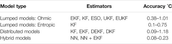
TABLE 5. Comparison of soft sensors.

3.4 Common Challenges and Benefits of Soft Sensors

As is evident from the various estimators that are discussed above, proper parameterization is of paramount importance similar to the model accuracy. As the estimation accuracy highly depends on the parameters, especially the internal resistance of the cell, parameterization tests need to be done for all possible scenarios to be sufficiently representative. Similarly, the validation tests should be well representative of the battery usage during actual charging, discharging, and resting conditions. Only a few studies have used a collection of various established driving cycles, the other studies have used either a single specific driving cycle or specific tests that are less representative. Therefore, the estimation accuracy of these soft sensors could decrease in real battery usage scenarios. However, the estimators that have been validated through various driving cycles show that these can be of high accuracy. Although this dependency on parameterization and validation test conditions is a major challenge, it can be overcome by the proper use of relevant tests.

Both types of sensors need to be properly calibrated offline, before installation and during routine maintenance. However, an additional challenge with soft sensors is that it needs an actual internal temperature measurement of a hard sensor (or an already tuned soft sensor) for the calibration. Furthermore, the estimation accuracy depends on the accuracy and precision of the other measurements that are used (such as surface temperature measurement and current); therefore, the soft sensor would not be of higher accuracy than the other sensors that are used.

Soft sensors are generally considered to be of low cost, and low power compared to the hard sensors, which allows realization of more comprehensive monitoring networks. The non-destructive ability is also a huge benefit, as the proper sealing of the cell is ensured and any maintenance related to outer measurements or the system can be done without any opening of the cell. Similarly, any sensor bias or sensor faults that can occur are easily corrected either by calibration or by using embedded fault detection and diagnosis systems.

Another main benefit is that additional information on various parameters that are useful for SOC estimation, can be obtained from the estimators apart from the temperatures. Furthermore, the soft sensors are easy to add into other estimators in the BMS, such as SOC and SOH estimations. Also, the estimators can be easily re-arranged to work with various BMS control structures, whether it is inbuilt with estimators or not. This is beneficial in smart monitoring and control systems, such as the control of self-heating in cells or control of the cooling system in BMS, where the soft sensor can minimize the time delay due to sensor data transfer by hard sensors.

4 Future Trends in Thermal Sensing in Batteries

Integration of smart functionalities into the battery is one of the main visions in worldwide future battery innovation research (Edström, 2020). Among these, smart cells and smart battery packs are conceptualized as emerging techniques. The smart cell concept is an integrated design of a cell with its management system. Each cell has a cell-level BMS that monitors and controls the critical states and parameters, which is then integrated with the system-level smart battery pack BMS. This provides high modularity, plug-and-play integration, high scalability, and enhanced fault tolerance for packs (Wei et al., 2021).

The use of smart sensors that can self-monitor and communicate is a major component of these smart cells. A smart sensor would be able to measure and do digital processing and on-board diagnostics, and communicate with other systems. Soft sensors can easily be incorporated into smart sensors due to their generality and online applicability (Xiong et al., 2018). However, the cell-level controller must be able to handle the additional computational burden of the soft sensor, together with pre-processing, and decision-making (Wei et al., 2021). The use of cloud computing technology for computationally heavy tasks is one option.

Another option is to use a hard sensor to lift this burden by directly measuring the temperature and communicating with the smart sensor. Thin-film thermocouples and thermistors, portable EIS or FBG sensors are good candidates for this. However, the sensors must be well-developed to have frequent real-time measurements, communication, and durability conditions. Another good candidate is the micro-structured optical fibers, also known as photonic crystal fibers. These are optical fibers that obtain total internal reflection by manipulating the waveguide structure, unlike FBGs that rely on the change in refractive index of the bragg gratings. The air-hole patterns within the core determine the properties of the sensor; therefore the careful design of these patterns provides a possible way to measure both internal temperature and pressure independently within a single fiber. However, the manufacturing of these sensors is still in the early stages, and intensive research and development are needed for testing the feasibility of using these in future batteries (Edström, 2020).

Further, future hard and soft sensors need to be able to operate accurately and reliably in the presence of non-ignorable electromagnetic interference that will occur due to increased communications between many cell BMSs. The use of various sensor fusion methods is a good candidate for future techniques for smart sensors, where various hard and soft sensors are combined for better performance. Moreover, for the hard sensors, more development is needed on smaller sizes and better substrates for less interference to the cell, durability, and high tolerance to the corrosive environment (Fleming et al., 2019). Furthermore, the future batteries are to be of low manufacturing cost and minimal in life cycle impact, which should also be considered for the attached/embedded sensors.

Generally, embedded sensors need to be equipped with effective insulation, less thermal impact, high flexibility for distributed measurement, and long-term stability in addition to the above-mentioned abilities (Wei et al., 2021). These qualities should be able to be applied to future battery types and chemistries, such as solid-state and semi-solid-state batteries or silicon-based lithium-ion batteries. Similarly, for the soft sensors, the main development that is needed is the ability to accurately sense the distributed internal temperature. It will further be advantages if these are cheaper and faster than today.

5 Conclusion

In this review, the most recent studies on various online internal temperature monitoring techniques were reviewed under two main themes of hard sensors and soft sensors. Contact sensors such as thermocouples, thermistors, RTDs, and fiber optic sensors, and contactless sensors such as EIS and JNT are discussed under hard sensors. Physics model-based and hybrid method-based soft sensors are discussed under soft sensors, focusing on various types of models that are used. More weight is given to the soft sensors due to the lack of in-depth review studies on these. The sensor types are analyzed in detail with their accuracy, implementation, measurement frequency, and their common challenges and benefits. Furthermore, possible future trends in internal temperature sensing in future LIBs technologies are also discussed.

Generally, hard sensors are the most accurate; however, proper sealing methods are needed for embedding, and good insulation and protective layers are needed for the durability and reliability of the sensor. Typical soft sensors are non-destructive, flexible, low-cost, and low-power; however, proper parameterization and accurate additional measurements such as surface temperature, current, voltage are needed for the accuracy of the sensor. Both types of sensors need rapid advancements to cater to the future BMS requirements as well as future smart battery requirements.

Author Contributions

AJ and OB: Concept. AJ: Analysis and drafting of the manuscript. LS and MW: Editing and reviewing of the manuscript. JL, PS, AS, and OB: Critical revision of the manuscript. OB: Acquisition of funding. AS and OB: Project management and supervision.

Conflict of Interest

The authors declare that the research was conducted in the absence of any commercial or financial relationships that could be construed as a potential conflict of interest.

Publisher’s Note

All claims expressed in this article are solely those of the authors and do not necessarily represent those of their affiliated organizations, or those of the publisher, the editors and the reviewers. Any product that may be evaluated in this article, or claim that may be made by its manufacturer, is not guaranteed or endorsed by the publisher.

Acknowledgments

The authors acknowledge the support from the ENERSENSE research initiative at Norwegian University of Science and Technology, Norway. PS acknowledges the support of The Royal Academy of Engineering (CiET1718/59). AJ acknowledges the support from Freyr Battery AS, Norway and KeyTechNevo project at Norwegian University of Science and Technology, Norway. LS acknowledges funding from the Research Council of Norway, via the research project BattMarine (project no. 281005).

References

Al Hallaj, S., Maleki, H., Hong, J. S., and Selman, J. R. (1999). Thermal Modeling and Design Considerations of Lithium-Ion Batteries. J. Power Sourc. 83, 1–8. doi:10.1016/S0378-7753(99)00178-0

CrossRef Full Text | Google Scholar

Amietszajew, T., Fleming, J., Roberts, A. J., Widanage, W. D., Greenwood, D., Kok, M. D. R., et al. (2019). Hybrid Thermo‐Electrochemical In Situ Instrumentation for Lithium‐Ion Energy Storage. Batteries & Supercaps 2, 934–940. doi:10.1002/batt.201900109

CrossRef Full Text | Google Scholar

Amietszajew, T., McTurk, E., Fleming, J., and Bhagat, R. (2018). Understanding the Limits of Rapid Charging Using Instrumented Commercial 18650 High-Energy Li-Ion Cells. Electrochimica Acta 263, 346–352. doi:10.1016/j.electacta.2018.01.076

CrossRef Full Text | Google Scholar

An, Z., Jia, L., Wei, L., Dang, C., and Peng, Q. (2018). Investigation on Lithium-Ion Battery Electrochemical and thermal Characteristic Based on Electrochemical-thermal Coupled Model. Appl. Therm. Eng. 137, 792–807. doi:10.1016/j.applthermaleng.2018.04.014

CrossRef Full Text | Google Scholar

Anthony, D., Wong, D., Wetz, D., and Jain, A. (2017). Non-invasive Measurement of Internal Temperature of a Cylindrical Li-Ion Cell during High-Rate Discharge. Int. J. Heat Mass Transfer 111, 223–231. doi:10.1016/j.ijheatmasstransfer.2017.03.095

CrossRef Full Text | Google Scholar

Babaeiyazdi, I., Rezaei-Zare, A., and Shokrzadeh, S. (2021). State of Charge Prediction of EV Li-Ion Batteries Using EIS: A Machine Learning Approach. Energy 223, 120116. doi:10.1016/j.energy.2021.120116

CrossRef Full Text | Google Scholar

Bandhauer, T. M., Garimella, S., and Fuller, T. F. (2011). A Critical Review of Thermal Issues in Lithium-Ion Batteries. J. Electrochem. Soc. 158, R1–R25. doi:10.1149/1.3515880

CrossRef Full Text | Google Scholar

Bolsinger, C., and Birke, K. P. (2019). Effect of Different Cooling Configurations on thermal Gradients inside Cylindrical Battery Cells. J. Energ. Storage 21, 222–230. doi:10.1016/j.est.2018.11.030

CrossRef Full Text | Google Scholar

Burheim, O. S., Onsrud, M. A., Pharoah, J. G., Vullum-Bruer, F., and Vie, P. J. S. (2014). Thermal Conductivity, Heat Sources and Temperature Profiles of Li-Ion Batteries. ECS Trans. 58, 145–171. doi:10.1149/05848.0145ecst

CrossRef Full Text | Google Scholar

Cao, J., and Emadi, A. (2011). Batteries Need Electronics. EEE Ind. Electron. Mag. 5, 27–35. doi:10.1109/mie.2011.940251

CrossRef Full Text | Google Scholar

Chalise, D., Shah, K., Halama, T., Komsiyska, L., and Jain, A. (2017). An Experimentally Validated Method for Temperature Prediction during Cyclic Operation of a Li-Ion Cell. Int. J. Heat Mass Transfer 112, 89–96. doi:10.1016/j.ijheatmasstransfer.2017.04.115

CrossRef Full Text | Google Scholar

Chen, G., Liu, Z., Su, H., and Zhuang, W. (2021). Electrochemical-distributed thermal Coupled Model-Based State of Charge Estimation for Cylindrical Lithium-Ion Batteries. Control. Eng. Pract. 109, 104734. doi:10.1016/j.conengprac.2021.104734

CrossRef Full Text | Google Scholar

Cheng, X., and Pecht, M. (2017). In Situ stress Measurement Techniques on Li-Ion Battery Electrodes: A Review. Energies 10, 591. doi:10.3390/en10050591

CrossRef Full Text | Google Scholar

Childs, P. R. N., Greenwood, J. R., and Long, C. A. (2000). Review of Temperature Measurement. Rev. Scientific Instr. 71, 2959–2978. doi:10.1063/1.1305516

CrossRef Full Text | Google Scholar

Debert, M., Colin, G., Bloch, G., and Chamaillard, Y. (2013). An Observer Looks at the Cell Temperature in Automotive Battery Packs. Control. Eng. Pract. 21, 1035–1042. doi:10.1016/j.conengprac.2013.03.001

CrossRef Full Text | Google Scholar

Ding, F., and Chen, T. (2005). Identification of Hammerstein Nonlinear ARMAX Systems. Automatica 41, 1479–1489. doi:10.1016/j.automatica.2005.03.026

CrossRef Full Text | Google Scholar

Duff, M., and Towey, J. (2010). Two Ways to Measure Temperature Using Thermocouples Feature Simplicity, Accuracy, and Flexibility. Analog Dialogue 44, 1–6.

Google Scholar

Edström, K. (2020). Inventing the Sustainable Batteries of the Future: Research Needs and Future Actions. Uppsala: battery2030+. Tech. rep.

Google Scholar

Farag, M., Sweity, H., Fleckenstein, M., and Habibi, S. (2017). Combined Electrochemical, Heat Generation, and thermal Model for Large Prismatic Lithium-Ion Batteries in Real-Time Applications. J. Power Sourc. 360, 618–633. doi:10.1016/j.jpowsour.2017.06.031

CrossRef Full Text | Google Scholar

Fleming, J., Amietszajew, T., Charmet, J., Roberts, A. J., Greenwood, D., and Bhagat, R. (2019). The Design and Impact of In-Situ and Operando thermal Sensing for Smart Energy Storage. J. Energ. Storage 22, 36–43. doi:10.1016/j.est.2019.01.026

CrossRef Full Text | Google Scholar

Fleming, J., Amietszajew, T., McTurk, E., Towers, D. P., Greenwood, D., and Bhagat, R. (2018). Development and Evaluation of In-Situ Instrumentation for Cylindrical Li-Ion Cells Using Fibre Optic Sensors. HardwareX 3, 100–109. doi:10.1016/j.ohx.2018.04.001

CrossRef Full Text | Google Scholar

Fortier, A., Tsao, M., Williard, N., Xing, Y., and Pecht, M. (2017). Preliminary Study on Integration of Fiber Optic Bragg Grating Sensors in Li-Ion Batteries and In Situ Strain and Temperature Monitoring of Battery Cells. Energies 10, 838. doi:10.3390/en10070838

CrossRef Full Text | Google Scholar

Fortuna, L., Graziani, S., Rizzo, A., and Xibilia, M. G. (2007). Soft Sensors for Monitoring and Control of Industrial Processes. London: Springer. doi:10.1007/978-1-84628-480-9Soft Sensors for Monitoring and Control of Industrial Processes

CrossRef Full Text | Google Scholar

Guo, B.-Z., and Zhao, Z.-L. (2011). “Extended State Observer for Nonlinear Systems with Uncertainty,” in IFAC Proceedings Volumes (IFAC-PapersOnline) (Milan, Italy: IFAC), 44, 1855–1860. doi:10.3182/20110828-6-IT-1002.00399IFAC Proc. Volumes

CrossRef Full Text | Google Scholar

Hofmann, A., Uhlmann, N., Ziebert, C., Wiegand, O., Schmidt, A., and Hanemann, T. (2017). Preventing Li-Ion Cell Explosion during thermal Runaway with Reduced Pressure. Appl. Therm. Eng. 124, 539–544. doi:10.1016/j.applthermaleng.2017.06.056

CrossRef Full Text | Google Scholar

How, D. N. T., Hannan, M. A., Hossain Lipu, M. S., and Ker, P. J. (2019). State of Charge Estimation for Lithium-Ion Batteries Using Model-Based and Data-Driven Methods: A Review. IEEE Access 7, 136116–136136. doi:10.1109/access.2019.2942213

CrossRef Full Text | Google Scholar

Hu, X., Liu, W., Lin, X., Xie, Y., Foley, A. M., and Hu, L. (2021). A Control-Oriented Electrothermal Model for Pouch-type Electric Vehicle Batteries. IEEE Trans. Power Electron. 36, 5530–5544. doi:10.1109/TPEL.2020.3027561

CrossRef Full Text | Google Scholar

Huang, J., Albero Blanquer, L., Bonefacino, J., Logan, E. R., Alves Dalla Corte, D., Delacourt, C., et al. (2020). Operando Decoding of Chemical and thermal Events in Commercial Na(Li)-Ion Cells via Optical Sensors. Nat. Energ. 5, 674–683. doi:10.1038/s41560-020-0665-y

CrossRef Full Text | Google Scholar

Kashyap, R. (1999). “Introduction,” in Fiber Bragg Gratings (San Diego: Academic Press), 1–12. chap. doi:10.1016/b978-012400560-0/50002-6

CrossRef Full Text | Google Scholar

Kersey, A. D. (1996). A Review of Recent Developments in Fiber Optic Sensor Technology. Opt. Fiber Technology 2, 291–317. doi:10.1006/ofte.1996.0036

CrossRef Full Text | Google Scholar

Kersey, A. D., Davis, M. A., Patrick, H. J., LeBlanc, M., Koo, K. P., Askins, C. G., et al. (1997). Fiber Grating Sensors. J. Lightwave Technol. 15, 1442–1463. doi:10.1109/50.618377

CrossRef Full Text | Google Scholar

Khan, M., Swierczynski, M., and Kær, S. (2017). Towards an Ultimate Battery thermal Management System: A Review. Batteries 3, 9. doi:10.3390/batteries3010009

CrossRef Full Text | Google Scholar

Lee, C.-Y., Lee, S.-J., Tang, M.-S., and Chen, P.-C. (2011). In Situ monitoring of Temperature inside Lithium-Ion Batteries by Flexible Micro Temperature Sensors. Sensors 11, 9942–9950. doi:10.3390/s111009942

PubMed Abstract | CrossRef Full Text | Google Scholar

Li, S., He, H., and Li, J. (2019). Big Data Driven Lithium-Ion Battery Modeling Method Based on SDAE-ELM Algorithm and Data Pre-processing Technology. Appl. Energ. 242, 1259–1273. doi:10.1016/j.apenergy.2019.03.154

CrossRef Full Text | Google Scholar

Li, Z., Zhang, J., Wu, B., Huang, J., Nie, Z., Sun, Y., et al. (2013). Examining Temporal and Spatial Variations of Internal Temperature in Large-Format Laminated Battery with Embedded Thermocouples. J. Power Sourc. 241, 536–553. doi:10.1016/j.jpowsour.2013.04.117

CrossRef Full Text | Google Scholar

Liao, Z., Zhang, S., Li, K., Zhang, G., and Habetler, T. G. (2019). A Survey of Methods for Monitoring and Detecting thermal Runaway of Lithium-Ion Batteries. J. Power Sourc. 436, 226879. doi:10.1016/j.jpowsour.2019.226879

CrossRef Full Text | Google Scholar

Liu, K., Li, K., and Deng, J. (2016). “A Novel Hybrid Data-Driven Method for Li-Ion Battery Internal Temperature Estimation,” in UKACC International Conference on Control (Belfast, UK: IEEE), 1–6. doi:10.1109/CONTROL.2016.7737560

CrossRef Full Text | Google Scholar

Liu, K., Li, K., Peng, Q., Guo, Y., and Zhang, L. (2018a). Data-driven Hybrid Internal Temperature Estimation Approach for Battery thermal Management. Complexity 2018, 1–15. doi:10.1155/2018/9642892

CrossRef Full Text | Google Scholar

Liu, K., Li, K., Peng, Q., and Zhang, C. (2019). A Brief Review on Key Technologies in the Battery Management System of Electric Vehicles. Front. Mech. Eng. 14, 47–64. doi:10.1007/s11465-018-0516-8

CrossRef Full Text | Google Scholar

Liu, X., Zheng, C., Liu, C., and Pong, P. W. T. (2018b). Experimental Investigation of a Johnson Noise Thermometry Using GMR Sensor for Electric Vehicle Applications. IEEE Sensors J. 18, 3098–3107. doi:10.1109/JSEN.2018.2805309

CrossRef Full Text | Google Scholar

Ma, S., Jiang, M., Tao, P., Song, C., Wu, J., Wang, J., et al. (2018). Temperature Effect and thermal Impact in Lithium-Ion Batteries: A Review. Prog. Nat. Sci. Mater. Int. 28, 653–666. doi:10.1016/j.pnsc.2018.11.002

CrossRef Full Text | Google Scholar

Ma, Y., Cui, Y., Mou, H., Gao, J., and Chen, H. (2020). Core Temperature Estimation of Lithium-Ion Battery for EVs Using Kalman Filter. Appl. Therm. Eng. 168, 114816. doi:10.1016/j.applthermaleng.2019.114816

CrossRef Full Text | Google Scholar

Martiny, N., Hornung, A., Schussler, M., and Jossen, A. (2014). “A Capacitively Coupled Data Transmission System for Resistance Based Sensor Arrays for In-Situ Monitoring of Lithium-Ion Battery Cells,” in Proceedings of IEEE Sensors, Valencia, Spain, 2-5 Nov. 2014 (IEEE), 535–538. doi:10.1109/ICSENS.2014.6985053

CrossRef Full Text | Google Scholar

McTurk, E., Amietszajew, T., Fleming, J., and Bhagat, R. (2018). Thermo-electrochemical Instrumentation of Cylindrical Li-Ion Cells. J. Power Sourc. 379, 309–316. doi:10.1016/j.jpowsour.2018.01.060

CrossRef Full Text | Google Scholar

Mehne, J., and Nowak, W. (2017). Improving Temperature Predictions for Li-Ion Batteries: Data Assimilation with a Stochastic Extension of a Physically-Based, Thermo-Electrochemical Model. J. Energ. Storage 12, 288–296. doi:10.1016/j.est.2017.05.013

CrossRef Full Text | Google Scholar

Mehne, J., and Nowak, W. (2018). Predicting the Battery Core Temperature: Explanatory Power of Measurement Quantities under Different Uncertainty Scenarios. J. Energ. Storage 18, 476–484. doi:10.1016/j.est.2018.06.001

CrossRef Full Text | Google Scholar

Modrzynski, C., Roscher, V., Rittweger, F., Ghannoum, A., Nieva, P., and Riemschneider, K.-R. (2019). “Integrated Optical Fibers for Simultaneous Monitoring of the Anode and the Cathode in Lithium Ion Batteries,” in Proceedings of IEEE Sensors (IEEE), Montreal, QC, Canada, 2019-Octob (IEEE), 1–4. doi:10.1109/SENSORS43011.2019.8956755

CrossRef Full Text | Google Scholar

Mutyala, M. S. K., Zhao, J., Li, J., Pan, H., Yuan, C., and Li, X. (2014). In-situ Temperature Measurement in Lithium Ion Battery by Transferable Flexible Thin Film Thermocouples. J. Power Sourc. 260, 43–49. doi:10.1016/j.jpowsour.2014.03.004

CrossRef Full Text | Google Scholar

Nascimento, M., Ferreira, M. S., and Pinto, J. L. (2017). Real Time thermal Monitoring of Lithium Batteries with Fiber Sensors and Thermocouples: A Comparative Study. Measurement 111, 260–263. doi:10.1016/j.measurement.2017.07.049

CrossRef Full Text | Google Scholar

Nascimento, M., Novais, S., Ding, M. S., Ferreira, M. S., Koch, S., Passerini, S., et al. (2019). Internal Strain and Temperature Discrimination with Optical Fiber Hybrid Sensors in Li-Ion Batteries. J. Power Sourc. 410-411, 1–9. doi:10.1016/j.jpowsour.2018.10.096

CrossRef Full Text | Google Scholar

Novais, S., Nascimento, M., Grande, L., Domingues, M., Antunes, P., Alberto, N., et al. (2016). Internal and External Temperature Monitoring of a Li-Ion Battery with Fiber Bragg Grating Sensors. Sensors 16, 1394–1399. doi:10.3390/s16091394

PubMed Abstract | CrossRef Full Text | Google Scholar

Parekh, M. H., Li, B., Palanisamy, M., Adams, T. E., Tomar, V., and Pol, V. G. (2020). In Situ Thermal Runaway Detection in Lithium-Ion Batteries with an Integrated Internal Sensor. ACS Appl. Energ. Mater. 3, 7997–8008. doi:10.1021/acsaem.0c01392

CrossRef Full Text | Google Scholar

Peng, J., Jin, Y., Jia, S., and Xu, S. (2020). “External Electrode Temperature Monitoring of Lithium Iron Phosphate Batteries Based on Fiber Bragg Grating Sensors,” in IOP Conference Series: Earth and Environmental Science, Sanya, China, 12-15 March 2020, 012002. doi:10.1088/1755-1315/495/1/012002IOP Conf. Ser. Earth Environ. Sci.495

CrossRef Full Text | Google Scholar

Raijmakers, L. H. J., Danilov, D. L., Eichel, R.-A., and Notten, P. H. L. (2019). A Review on Various Temperature-Indication Methods for Li-Ion Batteries. Appl. Energ. 240, 918–945. doi:10.1016/j.apenergy.2019.02.078

CrossRef Full Text | Google Scholar

Rath, S., Hoedemaekers, E. R. G., and Wilkins, S. (2020). “Core Temperature Estimation for a Cylindrical Cell Battery Module,” in 15th International Conference on Ecological Vehicles and Renewable Energies, EVER 2020, 1–10. doi:10.1109/EVER48776.2020.9243110

CrossRef Full Text | Google Scholar

Richardson, R. R., and Howey, D. A. (2015). Sensorless Battery Internal Temperature Estimation Using a Kalman Filter with Impedance Measurement. IEEE Trans. Sustain. Energ. 6, 1190–1199. doi:10.1109/TSTE.2015.2420375

CrossRef Full Text | Google Scholar

Richardson, R. R., Ireland, P. T., and Howey, D. A. (2014). Battery Internal Temperature Estimation by Combined Impedance and Surface Temperature Measurement. J. Power Sourc. 265, 254–261. doi:10.1016/j.jpowsour.2014.04.129

CrossRef Full Text | Google Scholar

Richardson, R. R., Zhao, S., and Howey, D. A. (2016a). On-board Monitoring of 2-D Spatially-Resolved Temperatures in Cylindrical Lithium-Ion Batteries: Part II. State Estimation via Impedance-Based Temperature Sensing. J. Power Sourc. 327, 726–735. doi:10.1016/j.jpowsour.2016.06.104

CrossRef Full Text | Google Scholar

Richardson, R. R., Zhao, S., and Howey, D. A. (2016b). On-board Monitoring of 2-D Spatially-Resolved Temperatures in Cylindrical Lithium-Ion Batteries: Part I. Low-Order thermal Modelling. J. Power Sourc. 326, 377–388. doi:10.1016/j.jpowsour.2016.06.103

CrossRef Full Text | Google Scholar

Rogers, A. (1999). Distributed Optical-Fibre Sensing. Meas. Sci. Technol. 10, R75–R99. doi:10.1088/0957-0233/10/8/201

CrossRef Full Text | Google Scholar

Schmidt, J. P., Arnold, S., Loges, A., Werner, D., Wetzel, T., and Ivers-Tiffée, E. (2013). Measurement of the Internal Cell Temperature via Impedance: Evaluation and Application of a New Method. J. Power Sourc. 243, 110–117. doi:10.1016/j.jpowsour.2013.06.013

CrossRef Full Text | Google Scholar

Shirazi, A. H. N., Azadi Kakavand, M. R., and Rabczuk, T. (2015). Numerical Study of Composite Electrode's Particle Size Effect on the Electrochemical and Heat Generation of a Li-Ion Battery. J. Nanotechnology Eng. Med. 6, 041003. doi:10.1115/1.4032012

CrossRef Full Text | Google Scholar

Spitthoff, L., Gunnarshaug, A. F., Bedeaux, D., Burheim, O., and Kjelstrup, S. (2021). Peltier Effects in Lithium-Ion Battery Modeling. J. Chem. Phys. 154, 114705. doi:10.1063/5.0038168

CrossRef Full Text | Google Scholar

Srinivasan, R., Carkhuff, B. G., Butler, M. H., and Baisden, A. C. (2011). Instantaneous Measurement of the Internal Temperature in Lithium-Ion Rechargeable Cells. Electrochimica Acta 56, 6198–6204. doi:10.1016/j.electacta.2011.03.136

CrossRef Full Text | Google Scholar

Srinivasan, R., Demirev, P. A., Carkhuff, B. G., Santhanagopalan, S., Jeevarajan, J. A., and Barrera, T. P. (2020). Review-Thermal Safety Management in Li-Ion Batteries: Current Issues and Perspectives. J. Electrochem. Soc. 167, 140516. doi:10.1149/1945-7111/abc0a5

CrossRef Full Text | Google Scholar

Sun, L., Sun, W., and You, F. (2020). Core Temperature Modelling and Monitoring of Lithium-Ion Battery in the Presence of Sensor Bias. Appl. Energ. 271, 115243. doi:10.1016/j.apenergy.2020.115243

CrossRef Full Text | Google Scholar

Thomas, K. E., and Newman, J. (2003). Thermal Modeling of Porous Insertion Electrodes. J. Electrochem. Soc. 150, A176. doi:10.1149/1.1531194

CrossRef Full Text | Google Scholar

Vergori, E., and Yu, Y. (2019). Monitoring of Li-Ion Cells with Distributed Fibre Optic Sensors. Proced. Struct. Integrity 24, 233–239. doi:10.1016/j.prostr.2020.02.020

CrossRef Full Text | Google Scholar

Waag, W., Käbitz, S., and Sauer, D. U. (2013). Experimental Investigation of the Lithium-Ion Battery Impedance Characteristic at Various Conditions and Aging States and its Influence on the Application. Appl. Energ. 102, 885–897. doi:10.1016/j.apenergy.2012.09.030

CrossRef Full Text | Google Scholar

Waldmann, T., Wilka, M., Kasper, M., Fleischhammer, M., and Wohlfahrt-Mehrens, M. (2014). Temperature Dependent Ageing Mechanisms in Lithium-Ion Batteries - A Post-Mortem Study. J. Power Sourc. 262, 129–135. doi:10.1016/j.jpowsour.2014.03.112

CrossRef Full Text | Google Scholar

Wan, E. A., and Nelson, A. T. (2001). “Dual Extended Kalman Filter Methods,” in Kalman Filtering and Neural Networks. Editor S. Haykin (New York: John Wiley & Sons). chap. 5. 123–173.

Google Scholar

Wang, M., and Li, H.-X. (2017). Real-Time Estimation of Temperature Distribution for Cylindrical Lithium-Ion Batteries under Boundary Cooling. IEEE Trans. Ind. Electron. 64, 2316–2324. doi:10.1109/TIE.2016.2624720

CrossRef Full Text | Google Scholar

Wang, P., Zhang, X., Yang, L., Zhang, X., Yang, M., Chen, H., et al. (2016). Real-time Monitoring of Internal Temperature Evolution of the Lithium-Ion coin Cell Battery during the Charge and Discharge Process. Extreme Mech. Lett. 9, 459–466. doi:10.1016/j.eml.2016.03.013

CrossRef Full Text | Google Scholar

Wei, Z., Zhao, J., He, H., Ding, G., Cui, H., and Liu, L. (2021). Future Smart Battery and Management: Advanced Sensing from External to Embedded Multi-Dimensional Measurement. J. Power Sourc. 489, 229462. doi:10.1016/j.jpowsour.2021.229462

CrossRef Full Text | Google Scholar

Westerhoff, U., Kroker, T., Kurbach, K., and Kurrat, M. (2016). Electrochemical Impedance Spectroscopy Based Estimation of the State of Charge of Lithium-Ion Batteries. J. Energ. Storage 8, 244–256. doi:10.1016/j.est.2016.09.001

CrossRef Full Text | Google Scholar

Xiao, Y. (2015). Model-Based Virtual Thermal Sensors for Lithium-Ion Battery in EV Applications. IEEE Trans. Ind. Electron. 62, 3112–3122. doi:10.1109/TIE.2014.2386793

CrossRef Full Text | Google Scholar

Xie, Y., Li, J., and Yuan, C. (2014). Mathematical Modeling of the Electrochemical Impedance Spectroscopy in Lithium Ion Battery Cycling. Electrochimica Acta 127, 266–275. doi:10.1016/j.electacta.2014.02.035

CrossRef Full Text | Google Scholar

Xie, Y., Li, W., Hu, X., Lin, X., Zhang, Y., Dan, D., et al. (2020). An Enhanced Online Temperature Estimation for Lithium-Ion Batteries. IEEE Trans. Transp. Electrific. 6, 375–390. doi:10.1109/TTE.2020.2980153

CrossRef Full Text | Google Scholar

Xiong, R., Li, L., and Tian, J. (2018). Towards a Smarter Battery Management System: A Critical Review on Battery State of Health Monitoring Methods. J. Power Sourc. 405, 18–29. doi:10.1016/j.jpowsour.2018.10.019

CrossRef Full Text | Google Scholar

Xue, W., Bai, W., Yang, S., Song, K., Huang, Y., and Xie, H. (2015). ADRC with Adaptive Extended State Observer and its Application to Air-Fuel Ratio Control in Gasoline Engines. IEEE Trans. Ind. Electron. 62, 5847–5857. doi:10.1109/TIE.2015.2435004

CrossRef Full Text | Google Scholar

Yan, B., Lim, C., Yin, L., and Zhu, L. (2013). Simulation of Heat Generation in a Reconstructed Licoo2 Cathode during Galvanostatic Discharge. Electrochimica Acta 100, 171–179. doi:10.1016/j.electacta.2013.03.132

CrossRef Full Text | Google Scholar

Yang, G., Leitão, C., Li, Y., Pinto, J., and Jiang, X. (2013). Real-time Temperature Measurement with Fiber Bragg Sensors in Lithium Batteries for Safety Usage. Measurement 46, 3166–3172. doi:10.1016/j.measurement.2013.05.027

CrossRef Full Text | Google Scholar

Yang, H., Amiruddin, S., Bang, H. J., Sun, Y. K., and Prakash, J. (2006). A Review of Li-Ion Cell Chemistries and Their Potential Use in Hybrid Electric Vehicles. J. Ind. Eng. Chem. 12, 12–38.

Google Scholar

Youngki Kim, Y., Mohan, S., Siegel, J. B., Stefanopoulou, A. G., and Yi Ding, Y. (2014). The Estimation of Temperature Distribution in Cylindrical Battery Cells under Unknown Cooling Conditions. IEEE Trans. Contr. Syst. Technol. 22, 2277–2286. doi:10.1109/TCST.2014.2309492

CrossRef Full Text | Google Scholar

Youngki Kim, Y., Siegel, J. B., and Stefanopoulou, A. G. (2013). “A Computationally Efficient thermal Model of Cylindrical Battery Cells for the Estimation of Radially Distributed Temperatures,” in American Control Conference (Washington: IEEE), 698–703. doi:10.1109/acc.2013.6579917

CrossRef Full Text | Google Scholar

Yuksel, K., Wuilpart, M., Moeyaert, V., and Megret, P. (2009). “Optical Frequency Domain Reflectometry: A Review,” in 2009 11th International Conference on Transparent Optical Networks, Ponta Delgada, Portugal, 28 June-2 July 2009 (IEEE), 1–5. doi:10.1109/ICTON.2009.5185111

CrossRef Full Text | Google Scholar

Zhang, C., Li, K., and Deng, J. (2016). Real-time Estimation of Battery Internal Temperature Based on a Simplified Thermoelectric Model. J. Power Sourc. 302, 146–154. doi:10.1016/j.jpowsour.2015.10.052

CrossRef Full Text | Google Scholar

Zhang, C., Zhu, Y., Dong, G., and Wei, J. (2019). Data‐driven Lithium‐ion Battery States Estimation Using Neural Networks and Particle Filtering. Int. J. Energ. Res 43, 8230–8241. doi:10.1002/er.4820

CrossRef Full Text | Google Scholar

Zhang, G., Cao, L., Ge, S., Wang, C.-Y., Shaffer, C. E., and Rahn, C. D. (2014). In Situ Measurement of Radial Temperature Distributions in Cylindrical Li-Ion Cells. J. Electrochem. Soc. 161, A1499–A1507. doi:10.1149/2.0051410jes

CrossRef Full Text | Google Scholar

Zhang, J., Yang, X.-G., Sun, F., Wang, Z., and Wang, C.-Y. (2020). An Online Heat Generation Estimation Method for Lithium-Ion Batteries Using Dual-Temperature Measurements. Appl. Energ. 272, 115262. doi:10.1016/j.apenergy.2020.115262

CrossRef Full Text | Google Scholar

Zhou, X., and Huang, J. (2020). Impedance-Based Diagnosis of Lithium Ion Batteries: Identification of Physical Parameters Using Multi-Output Relevance Vector Regression. J. Energ. Storage 31, 101629. doi:10.1016/j.est.2020.101629

CrossRef Full Text | Google Scholar

Zhu, C., Shang, Y., Lu, F., Jiang, Y., Cheng, C., and Mi, C. (2020a). Core Temperature Estimation for Self-Heating Automotive Lithium-Ion Batteries in Cold Climates. IEEE Trans. Ind. Inf. 16, 3366–3375. doi:10.1109/tii.2019.2960833

CrossRef Full Text | Google Scholar

Zhu, S., Han, J., An, H.-Y., Pan, T.-S., Wei, Y.-M., Song, W.-L., et al. (2020b). A Novel Embedded Method for In-Situ Measuring Internal Multi-point Temperatures of Lithium Ion Batteries. J. Power Sourc. 456, 227981. doi:10.1016/j.jpowsour.2020.227981

CrossRef Full Text | Google Scholar