Optimal Conversion of Organic Wastes to Value-Added Products: Toward a Sustainable Integrated Biorefinery in Denmark

1 Introduction

A linear economy that favors extraction, use, and disposal is no longer acceptable. It is increasingly clear that we have finite resources and that today’s production/consumption is tomorrow’s burden. Climate change, the ever-rising energy crisis, and resulting worldwide tension are unambiguous signs pushing the sustainable production and consumption agenda. The concept of circular economy (CE) arises from the need to decouple economic growth from climate change by encouraging closing the energy and materials loop and optimizing use (UnitedNations, 2019; Venkata Mohan et al., 2019). Furthermore, CE endorses the zero-waste policy and actively shifts the traditional paradigm into a bio-based reality (bioeconomy, Figure 1). It is vital to accomplish this as fast as possible; this is achieved through the development and implementation of biorefineries (Figure 1). Biorefining is typically defined as the conversion of biomass into various commodities and specialty chemicals that differ considerably depending on the feedstock (e.g., fuels and bioplastics, respectively) (Giuliano et al., 2016). Furthermore, thriving toward a sustainable and circular bio-economy, the concept of integrated biorefineries is gaining ground as a strategy to reduce waste and energy consumption due to its multi-product nature (Chemmangattuvalappil and Ng, 2013). It leads to producing a myriad of chemicals and fuels where the latter could be used in-house to cover part, if not all, of the plant’s energy requirements. Convincing parallels can be drawn between refining and biorefining Gargalo et al. (2017). However, to avoid the traditional pitfalls observed in the conventional refinery, efficient design, implementation, and operation strategies have to be put in place to attain sustainable production and economic growth. Therefore, research into bio-based avenues in the form of integrated biorefineries for the production of everyday commodities and specialty chemicals has been significantly rising. A current hurdle entails handling the uncertainty encircling this topic; various unknown factors, performance variation, and several process alternatives, among other factors, lead to a multitude of potential options concerning the design, operation, and product assortment to be supplied by biorefineries (Gargalo et al., 2017; Svensson et al., 2015). Thereupon, it is imperative to develop and implement efficient strategies for planning and implementing viable integrated biorefineries for future commercial applications starting at the very early stages of design. The two main approaches for early-stage conceptual design are hierarchical decomposition and superstructure optimization (Mencarelli et al., 2020; Chemmangattuvalappil et al., 2020). The latter is the most common strategy because it facilitates the systematic screening of design alternatives. This approach allows assessing and optimizing the processes’ performance from various perspectives using different objective functions (e.g., minimizing costs and environmental burden). However, there is a delicate balance between simplicity and detail to identify the optimal or a set of promising alternatives confidently. A crudely defined superstructure built on very limited details and processing pathways leads to a poor solution. It usually follows a standard set of steps: (i) define the goal, scope, and complexity of the problem (e.g., decisions on the level of detail, assumptions); (ii) compile a comprehensive library of process models and pertinent data; (iii) set up the superstructure of connections and processing routes; (iv) derive the problem’s mathematical formulation [constraints and objective function(s)]; and finally, (v) apply a numerical solver and identify the optimal solution(s). Superstructure-based optimization has consistently and successfully been applied throughout the years for biorefinery design and in the Process Systems Engineering (PSE) field in general. Therefore, there are many studies on the topic. Because the goal of this work is not to present an extensive literature review, examples of such efforts are here limited to works that (i) are carried out in the last decade (2011–2021); (ii) focus on the design and optimization of multi-product biorefineries by applying a superstructure-based mathematical optimization approach, (iii) use organic waste/biomass as feedstock, and (iv) are deterministic studies. These works are collected, analyzed, and benchmarked in Supplementary Table S1. As demonstrated in Supplementary Table S1, many studies focus primarily on the production of ethanol and biofuels. For example, early studies (Ponce-Ortega et al., 2012a; Gabriel and El-Halwagi, 2013) identified the best conversion pathways of LCF and different types of biomass into bio-alcohols, respectively. Other studies (Vikash and Shastri, 2019; Restrepo-Flórez and Maravelias, 2020) also focused their research on identifying the best routes for the production of ethanol and ethanol derivatives, having lignocellulosic feedstock (LCF) as the starting material. Although to a significantly lower degree, the early-stage design of biorefineries for the production of high-value-added chemicals and building blocks has also been explored. Early studies such as Zondervan et al. (2011b) analyzed the pathways for the conversion of LCF and crude oil into ethanol, butanol, succinic acid, and blends of these compounds with gasoline. A recent study by Elyasi et al. (2021) aimed to identify the best pathway for producing energy and chemicals from biomass. This work emphasizes building a comprehensive network of processing pathways and corresponding process data to convert LCF and other organic wastes (e.g., manure) into value-added chemicals and energy. To the best of our knowledge, we present the most extensive network of processing technologies, and corresponding models and data, for all stages of biomass conversion. The superstructure includes all available technologies for the different steps of biomass conversion (e.g., preprocessing, pretreatment, hydrolysis and fermentation, and purification). The value-added products used as the base case resulting from the conversion of LCF are succinic acid, lactic acid, and ethanol. Moreover, electricity, biogas, and steam are obtained from the conversion of manure and lignin and can ultimately be used to cover the plant’s needs. The production of these compounds acts as a showcase demonstration and reflects current needs (e.g., bioplastics precursors for fossil-plastics replacement). Furthermore, as presented in Supplementary Table S1, very few studies use multi-objective optimization (MOO) (6 out of 22 studies). The works that use MOO typically consider CO₂ emissions as the second objective function. Thus, the multi-faceted aspects of sustainability are rarely considered. This study applies MOO that explicitly integrates zero-waste and bio-based circular economy policies by aiming at closing the loop and optimizing use. To this end, one of the objective functions is defined as the E-factor, typically used in green chemistry (Sheldon, 2017), to address the minimization of waste in the whole facility. We believe that, by minimizing waste, we reduce some of the environmental impact and health hazards associated with waste disposal and thus contribute positively to the environmental and social aspects (e.g., soil acidification and health and safety of local communities, respectively). Furthermore, it is remarkable that 21 out of the 22 modeling and optimization studies reviewed in Supplementary Table S1 have used closed-source software (e.g., GAMS). Nevertheless, it is progressively important to support the use of open-source software and programming languages to encourage knowledge-sharing, standardization, and validation of models (Gargalo et al., 2021; Mencarelli et al., 2020). Overall, in the PSE field, as reviewed by Mencarelli et al. (2020), very few studies indeed focus on using open-source software and programming languages for process design and optimization. For example, Chen et al. (2018b) proposed the Pyomo.GDP modeling environment. Their study supported GDP modeling and thus can be used in different solution strategies Chen and Grossmann (2019a). In addition, Pyomo.GDP also used the IDAES model library (chemical processes), proposed by Lee et al. (2018), which uses Pyomo.Network. Notably, to the best of our knowledge, there are no open-source-based biomass biorefinery design and optimization studies. Therefore, this work stands out by proposing a fully open-source organic waste to value-added products (O2V) model and optimization tool (Pyomo, Python-based). O2V aims to aid/assist the transition from a linear economy to a zero-waste and circular bioeconomy. Thereby, O2V provides a quick and reliable strategy to identify the potential optimal set of design, planning, and operational decisions for developing and implementing sustainable organic waste-based integrated biorefineries. In summary, this study introduces the following novel aspects.

• It proposes the O2V model and (multi-)objective optimization tool to identify the best planning and design decisions for the development of an integrated organic waste-based biorefinery (e.g., product portfolio and technologies);

• It addresses the zero-waste and bio-based circular economy policies/initiatives by employing E-factor as one of the objective functions;

• It proposes, to the best of our knowledge, the most comprehensive network of processing pathways for the conversion of organic waste into value-added products (all LCF conversion steps are mathematically described);

• The model has been formulated in the “plug-and-play” setup; in other words, the addition of new data and products to the superstructure of alternatives is straightforward and does not require modifications to the mathematical formulation (the data are added to a structured database);

• The realistic case of developing and implementing a sustainable integrated biorefinery in Denmark is selected. This case is chosen as a showcase to demonstrate the model’s applicability due to the high availability of organic wastes (LCF and pig manure) in Denmark, thus making it possibly an ideal location for such a platform.

FIGURE 1

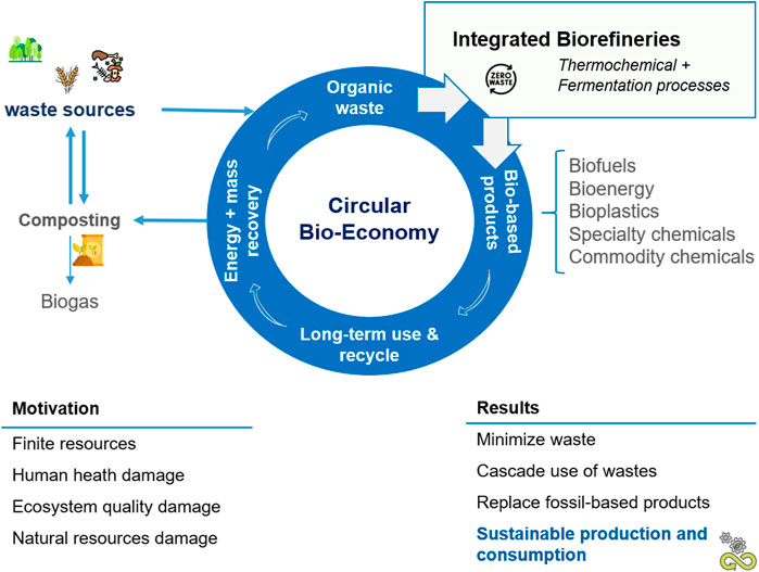
FIGURE 1. Circular bioeconomy: motivation, strategy, and results. Symbols from www.flaticon.com.

The remainder of the article is structured as follows. Section 2 describes the pathways for the conversion of organic waste into value-added products. It also provides details regarding data collection, superstructure generation, and the specifics concerning the implementation of an integrated biorefinery in Denmark. In Section 3, the O2V model is described and the mathematical formulation is defined. The results and discussion are presented in Section 4. Finally, conclusions and future perspectives are drawn in Section 5.

2 Organic Waste to Value-Added Products in Denmark: Toward a Realistic and Sustainable Integrated Biorefinery

The main objective of this work is to design a sustainable integrated biorefinery for the conversion of organic waste into value-added products. Denmark was selected as the location and thus the showcase. The data needed are collected (in a structured database) and presented in this section.

2.1 Availability of Organic Waste in Denmark

LCF availability in Denmark is expected to reach 4.5 million dry tons/year by 2030 (Panoutsou and Singh, 2020). Straw is the second biggest contributor to the total available LCF (1.367 million dry tons/year). Panoutsou and Singh (2020) presented that wheat straw and barley straw have the highest availability. In 2019, the annual production in Denmark was 2017 and 2580 million kg of barley and wheat straw, respectively (Denmark, 2020b). However, this total is not entirely available. Approximately 50% is not collected and the rest is mainly used to produce energy and feed (Nilsson et al., 2016). Pig manure is another significant source of organic waste in Denmark. A total of 12 million pigs were registered in Denmark (2020a). Considering an average of 4.1 kg of manure/swine per day (Losinger and Sampath, 2000), the total quantity of manure is approximately 18,000 million kilos per year. Therefore, wheat and barley straw are the LCF sources selected along with pig manure due to the aforementioned considerations. These are very promising feedstocks for the development and implementation of a sustainable integrated biorefinery in Denmark.

2.2 Value-Added Products From Organic Waste

2.2.1 Lignocellulosic Feedstock

Although the most common use of straw in Denmark is for energy production, its great potential for the production of chemicals and fuels is not explored. A certain set of steps are needed to convert the LCF into valuable products. The main step is to convert LCF into fermentable sugars: C₅ (e.g., xylose and arabinose) and C₆ (e.g., mainly glucose, mannose, galactose, and rhamnose) (Lee, 2015). These sugars can be converted through fermentation (biological) or chemical processing. An extensive analysis of fuels and platform chemicals that can be obtained from the conversion of LCF was presented by Isikgor and Becer (2015). It is necessary to reduce the portfolio of products to include in the superstructure of alternatives that will be analyzed in this study. Different criteria can be applied to choose the most promising product portfolio for the integrated biorefinery (Bozell and Petersen, 2010). To this end, some of the strategies are as follows: (i) to perform an extensive analysis of recent literature and reports (e.g., European Union, IEA tasks); (ii) to assess if the product has direct fossil-based counterparts (can be used as a direct substitute); (iii) to identify the product as a commodity (high volume) or specialty chemical/precursor/building block (high value); and (iv) to analyze the potential for commercialization and industrial scale-up (Bozell and Petersen, 2010). The primary motivation behind the choice of products is to design an integrated biorefinery capable of and effective in producing high-volume products (EtOH) and specialty high-value-added products (SA, LA). Lactic acid and succinic acid are bioplastic precursors with direct applications in pharmaceutics and cosmetics. Their production market demand has steadily increased over the years. Bio-based ethanol can directly replace fossil-based ethanol in most applications. Furthermore, it is worth noting that these chemicals have been thoroughly studied, and therefore the data available are trustworthy for further use in follow-up studies, such as this study. Hence, based on the mentioned criteria, realistic manure and LCF-based product portfolio were selected, and these products are ethanol (EtOH), lactic acid (LA), and succinic acid (SA). The main processing stages for the production of fermentation products from LCF are as follows: (i) preprocessing (Kumar et al., 2009; Aristizábal-Marulanda and Cardona Alzate, 2019); (ii) pretreatment (Kumar et al., 2009; Aristizábal-Marulanda and Cardona Alzate, 2019); (iii) detoxification (Aristizábal-Marulanda and Cardona Alzate, 2019; Vikash and Shastri, 2019); (iv) hydrolysis and fermentation (Gomez et al., 2008; Aristizábal-Marulanda and Cardona Alzate, 2019); and (v) purification and concentration (Komesu et al., 2017; Aristizábal-Marulanda and Cardona Alzate, 2019). More details are presented in Section 2.3.

2.2.2 Manure

There are two main processing avenues to convert manure into value-added products: (i) energy-oriented technologies, such as biogas production, gasification, and combustion, followed by hydrothermal liquefaction, and (ii) technologies that lead to other products such as composting, pyrolytic carbonization, or hydrothermal carbonization (Khoshnevisan et al., 2021). In Denmark, biogas production has quadrupled between 2012 and 2020, producing approximately 20 PJ/year Støckler et al. (2020), in which manure and organic waste are the two chief feedstocks. Therefore, this valorization pathway, manure to biogas, and biogas upgrading are options included in this study.

Of note is that the production of biogas and EtOH can be used in-house to cover part, if not all, of the facility’s energy needs and thus closing both energy and materials loops (zero-materials and zero-energy wastes).

2.3 Data Collection and Superstructure Generation

As mentioned above, the goal is to identify the optimal design and planning decisions for a realistic and sustainable integrated biorefinery in Denmark based on the conversion of organic wastes. To achieve this, the design and planning decisions to identify are as follows: (i) the production capacity of the set of products; (ii) the set of technologies in the five production sections for the LCF-based conversion; and (iii) the technologies for the conversion of manure and lignin. Furthermore, to the best of our knowledge, we propose the most comprehensive and detailed network of alternatives to produce ethanol, LA, SA, biogas, and electricity from manure, barley, and wheat straw. The superstructure of alternatives is presented in Figures 2, 3, for the conversion of LCF, manure, and lignin (a by-product of LCF processing), respectively. Notably, there are a few compatibility limitations among the processing steps, which are elaborated upon in the following subsections. Considering this, the number of available production pathways decreases. A detailed description of the processing steps, the data requirements, and the assumptions made are given in the following subsections. Furthermore, to apply the O2V model and optimization tool, the required data are stored in a structured database (see Figure 5).

• List of technologies for the conversion of feedstocks into final products;

• Process models and associated data/parameters (e.g., yields, conversion, and recovery factors);

• List of the compatibility and limitations among processing steps;

• Composition of the organic wastes (Supplementary Table S3);

• Total quantities of feedstock available to be converted;

• Prices of products, feedstocks, chemicals, and utilities (Supplementary Tables S9, S21).

Step 1: Preprocessing

FIGURE 2

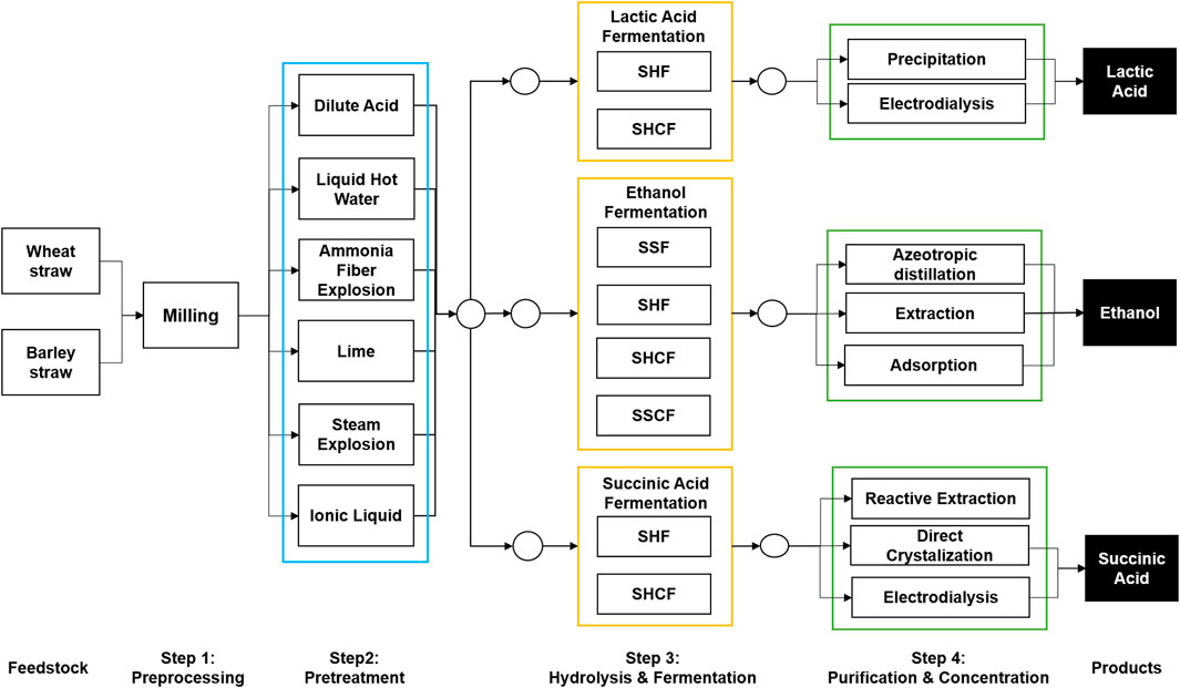
FIGURE 2. Superstructure of alternatives for the conversion of LCF into value-added products. SHF: separate hydrolysis and fermentation; SHCF: separate hydrolysis and co-fermentation; SSF: simultaneous saccharification and fermentation; SSCF: simultaneous saccharification and co-fermentation.

FIGURE 3

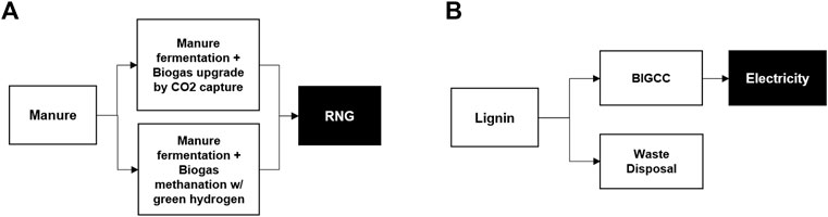
FIGURE 3. Superstructure of alternatives for the conversion of manure (A,B) lignin into value-added products. RNG: renewable natural gas-biogas; BIGCC: biomass integrated gasification combined cycle.

The preprocessing step aims to reduce the LCF biomass’s particle size before sending it to the pretreatment step. A maximum LCF biomass particle size characterizes the pretreatment technology in the inlet biomass. Thus, the pretreatment step imposes the preprocessing step’s particle size and energy consumption because a maximum input particle size characterizes the pretreatment step. This value is defined as the size at which the highest pretreatment efficiency is obtained, and any further decrease in size does not increase the efficiency of the process (Vikash and Shastri, 2019). In this work, a hammer mill is used to model this step. The energy consumption corresponding to the size reduction is based on the correlation presented by Kumar et al. (2009), which depends on the output particle size. These are presented in Supplementary Table S11.

Step 2: Pretreatment

This step aims to prepare the LCF to maximize the efficiency of the hydrolysis and fermentation stages. Thus, in this step, the porosity of the feedstock is amplified while dissolving lignin and hemicellulose, as well as reducing the cellulose’s crystallinity. Moreover, one of the main requirements is to minimize the formation of inhibitors (Kumar et al., 2009; Aristizábal-Marulanda and Cardona Alzate, 2019). There are different types and strategies (e.g., chemical and physical), which translate into the following pretreatment technologies: dilute acid, lime, ammonia fiber expansion (AFEX), liquid hot water (LHW), ionic liquid, and steam explosion. The recovery yields of the different species (cellulose, hemicellulose, and glucose) are reported in Supplementary Table S5.

Step 3: Hydrolysis and fermentation

The hydrolysis leads to the formation of fermentable sugars through enzymatic activity (cellulases and hemicellulases). Typically, the available commercial enzymes for saccharification and hydrolysis consist of a combination of several enzymes (Gomez et al., 2008). The required enzyme load for the hydrolysis, which depends on the preceding pretreatment stage, is given in Supplementary Table S14. Various organisms, such as bacteria and yeast (natural or engineered), can convert fermentable sugars into LA, SA, and ethanol (Di Lorenzo and Androsch, 2018). The strains are usually defined by their attainable titer (g/L), yield (g/g), and productivity (g/L/h). Supplementary Table S4 reports the bioconversion yields of fermentable sugars into products. The following hydrolysis and fermentation methods are considered in this work and hence included in the superstructure of alternatives: (a) separate hydrolysis and fermentation (SHF); (b) simultaneous saccharification and fermentation (SSF); (c) separate hydrolysis and co-fermentation (SHCF); and (d) simultaneous saccharification and co-fermentation (SSCF). A schematic representation of the main differences among the techniques is presented in Figure 4. The hydrolysis conversion factors for SHF and SHCF and the factors pertaining to the conversion of xylose to ethanol in SSCF and SSF are reported in Supplementary Table S6. The main traits and distinctions between the mentioned technologies are as follows.

FIGURE 4

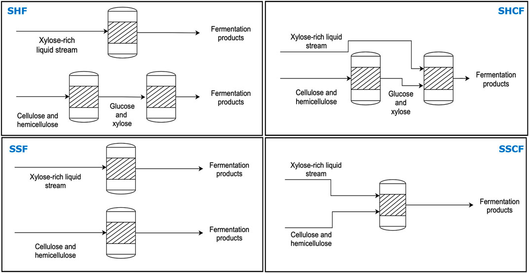
FIGURE 4. Hydrolysis and fermentation configurations.

SHF: the solid stream containing cellulose and hemicellulose obtained from Step 2 goes through hydrolysis, leading to a mixture of glucose and xylose. This stream is then led to the fermentation reactor. The xylose in the liquid stream from the pretreatment section is fermented in a separated bioreactor.

SSF: both solid and liquid streams exiting the pretreatment section enter two different bioreactors. Both undergo simultaneous hydrolysis and fermentation (one bioreactor for each stream).

SSHF: this technique is reminiscent of SHF; however, the xylose-rich liquid stream from pretreatment is mixed with the fermentable sugars from the hydrolysis of the solid stream. Thus, all the sugars obtained from both streams are fermented in one reactor.

SSCF: this technique is reminiscent of SSF. However, the xylose-rich liquid stream and the solid stream (mainly composed of cellulose and hemicellulose) are both sent to one reactor, where all the sugars are fermented.

Step 4: Product Purification and Concentration

The outlet of Step 3 is composed of main products (moderate-to-low concentration), by-products, and other species (e.g., non-fermented sugars). The unwanted compounds are removed in the purification and concentration step to reach the desired concentration and purity. To this end, documented technologies are, for example, precipitation, liquid–liquid extraction, and reactive distillation. Their implementation depends on the main product, and it is usually a compromise between energy and solvent consumption as well as the technology’s TRL (technology readiness level). Details on the available technologies are explored by Komesu et al. (2017). In this work, the following technologies are included:

LA purification and concentration: (i) precipitation → esterification → distillation; and (ii) electrodialysis → esterification → distillation.

SA purification and concentration: (i) electrodialysis, (ii) direct crystallization, and (iii) reactive extraction.

Ethanol purification and concentration: (i) distillation → extractive distillation with ethyl alcohol; (ii) distillation → azeotropic distillation with cyclohexane; and (iii) distillation → adsorption. The primary products’ recovery factors regarding the different purification and concentration technologies are presented in Supplementary Table S7. Supplementary Table S7 also illustrates the compatibility between the main product and Step 4’s technologies. In addition, the utilities required for this step are reported in Supplementary Tables S15–S17 for SA, LA, and ethanol, respectively.

2.3.1 Lignin and Manure Conversion

In this study, two options for the conversion of lignin are included in the superstructure: conversion of lignin into electricity using BIGCC technology (González-García et al., 2012), or lignin is disposed of as waste. The bioconversion of manure into biogas is achieved by applying one of the following technologies: (A) fermentation and biogas upgrade by CO₂ removal and (B) fermentation and biogas methanation using H₂ (electrolysis). The recovery factors for the manure and lignin conversion are reported in Supplementary Table S8. The data regarding the utilities and chemicals used in both lignin and manure conversion processes are reported in Supplementary Tables 18, 19.

3 O2V Model and Optimization Tool: Organic Waste to Value-Added Products

3.1 Model Outline

As previously mentioned, organic waste is a by-product of agro-activities, with a market price that is virtually zero. Thus, in order to thrive toward a circular bio-based and zero-waste economy, the upgrading of these wastes must/should not be overlooked. This study aims to identify and systematically investigate the optimal integrated biorefinery design(s) for converting organic waste into value-added products to aid and enable this paradigm shift. Therefore, in this work, as presented in Figure 5, we propose a modeling and optimization tool that aims to be accurate but also easy to apply for screening alternatives at the very early stages of design and decision-making.

FIGURE 5

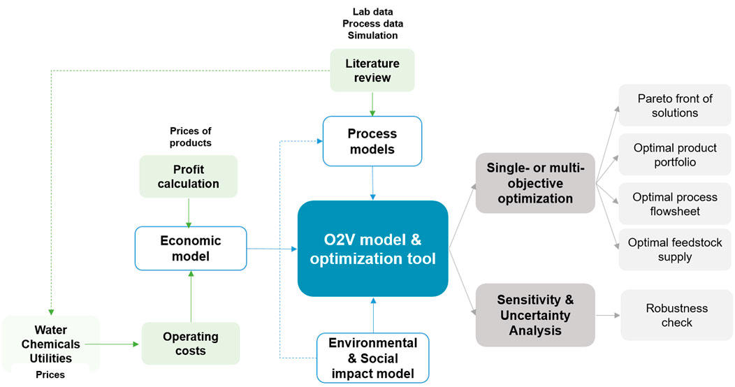
FIGURE 5. O2V model inputs and outputs.

O2V was built upon integrating (i) upstream and downstream processing models (black box models) for the conversion of organic waste into value-added products; (ii) technology selection and operational strategies; (iii) economic, environmental, and social modeling criteria; and (iv) a multi-objective optimization scheme. The problem is formally stated as follows:

Goal: To maximize the operating profit and minimize the E-factor of the integrated biorefinery.

Given:

• A superstructure of alternatives for the integrated biorefinery that composes the design space;

• Organic waste composition (LCF and manure);

• Available amounts of organic waste that are available (yearly supply fluctuation is disregarded);

• A set of value-added products that comprises the product portfolio;

• Process models (black box models);

• Market prices of products, by-products, chemicals, and utilities;

• Economic, environmental, and social models (operating profit and e-factor).

Detailed model assumptions:

• Only glucose and xylose are considered to be produced. Other sugars obtained from cellulose and hemicellulose are not considered because cellulose is a homopolymer of glucose, and xylose is the most abundant sugar in hemicellulosic fractions (70%–80%) Sun et al. (1996);

• The effect of inhibitors on the different fermentation yields is not considered; it is assumed that all by-products are removed after the pretreatment;

• All fermentation by-products are considered to be removed during the purification and concentration stages (not included in the model);

• All flows are estimated on a dry basis;

• Only operating costs are considered in the economic model; capital and storage costs are disregarded;

• The model does not optimize operating conditions;

• Process data are based on available literature. Thus, some data are obtained from lab-scale experiments and simulations (e.g., Aspen) and might not truly represent the processes at an industrial scale. This might lead to a biased comparison due to the lack of maturity of some technologies;

• In the AFEX and ionic liquid pretreatments, 90% of the ammonia is recycled and 1-ethyl-3-methylimidazolium acetate is 100% recycled, respectively;

• The detoxification stage is not modeled because there is not enough data to account for the effects of inhibitors. As previously mentioned, it is assumed that the inhibitors are removed and do not impact the following steps.

3.2 Mathematical Formulation

The O2V model is formulated as a generalized disjunctive programming (GDP) model for the optimization of the integrated biorefinery superstructure shown in Figures 2, 3. Constraints are defined according to the superstructure of connections to represent, for example, mass balances and capacity limitations. The comprehensive mathematical model formulation is detailed below (constraints and objective function). The complete list of indices, sets, parameters, and binary and continuous variables used is given in the Nomenclature Section.

3.2.1 Constraints

The production planning constraints concerning the selection of feedstock and technologies, mass balance relationships, and capacity constraints, among others, are presented in this section. The constraints and relationships are grouped into steps divided according to the biorefinery stages (Step 1: Preprocessing; Step 2: Pretreatment; Step 3: Bioconversion; and lastly, Step 4: Product purification and concentration). Furthermore, the constraints related to the lignin and manure conversion are also described in this section. The indices, sets, parameters, and binary and continuous variables used in the different steps are detailed in the corresponding tables.

Step 1: Preprocessing

The O2V model allows multiple feedstocks to be chosen simultaneously. The following disjunction describes the inflow of feedstocks into the production network:

$\left[\begin{array}{c}\hfill Y_{S_1}^{B_1}\left(b_1\right)\hfill \\ \hfill \sum _{c\in C}{F}_{S_1}\left(b_1,c\right)>0\hfill \end{array}\right]\vee \left[\begin{array}{c}\hfill \neg Y_{S_1}^{B_1}\left(b_1\right)\hfill \\ \hfill \sum _{c\in C}{F}_{S_1}\left(b_1,c\right)=0\hfill \end{array}\right]\forall b_1\in B_1,(1)$

where $Y_{S_1}^{B_1}(b_1)=1$ represents that feedstock b₁ ∈ B₁ is selected. Thus, the total amount of feedstock b₁ sent to the preprocessing stage is positive $(\sum _{c\in C}{F}_{S_1}(b_1,c)>0)$. Otherwise, when feedstock b₁ ∈ B₁ is not selected, the continuous variable representing the inflow of feedstock into the preprocessing stage is zero. Only one preprocessing technology can be chosen per feedstock b₁ ∈ B₁ as follows:

$\sum _{c\in C}{Y}_{S1}^{\mathit{Prep.}}\left(b_1,c\right)=Y_{S_1}^{B_1}\left(b_1\right)\forall b_1\in B_1,(2)$

Constraint (2) ensures that (i) the binary variable $Y_{S1}^{\mathit{Prep.}}(b_1,c)$ is activated only when the feedstock b₁ ∈ B₁ is selected and (ii) no preprocessing technology c ∈ C is chosen if there is no inflow of feedstock b₁ ∈ B₁ (b₁ not selected, $Y_{S_1}^{B_1}(b_1)=0$). Furthermore, Constraint (3) through the disjunction, expresses that when/if the preprocessing technology c is not selected $(Y_{S1}^{\mathit{Prep.}}(b_1,c)=0)$, the inflow of feedstock to that technology is 0. Else, if c is indeed chosen $(Y_{S1}^{\mathit{Prep.}}(b_1,c)=1)$, the inflow of into preprocessing stage c must be greater than zero $(F_{S_1}(b_1,c)>0)$.

$\left[\begin{array}{c}\hfill Y_{S_1}^{\mathit{Prep.}}\left(b_1,c\right)\hfill \\ \hfill F_{S_1}\left(b_1,c\right)>0\hfill \end{array}\right]\vee \left[\begin{array}{c}\hfill \neg Y_{S_1}^{\mathit{Prep.}}\left(b_1,c\right)\hfill \\ \hfill F_{S_1}\left(b_1,c\right)=0\hfill \end{array}\right]\forall b_1\in B_1,\forall c\in C.(3)$

Step 2: Pretreatment

The feedstock, after the preprocessing stage, can be distributed to different pretreatment technologies (d ∈ D); however, only one pretreatment technology can be assigned to a specific feedstock (b₁ ∈ B₁). This is represented by the following constraints:

$F_{S_1}\left(b_1,c\right)=\sum _{d\in D}{F}_{S_1\to S_2}\left(b_1,c,d\right)\forall b_1\in B_1,\forall c\in C(4)$

$\sum _{d\in D}{Y}_{S_2}\left(b_1,d\right)=Y_{S_1}^{B_1}\left(b_1\right)\forall b_1\in B_1(5)$

The mass balance between both processing steps is established in Constraints (4, 5), imposing that $Y_{S_2}(b_1,d)=1$ for only one d ∈ D, in the case where b ∈ B₁ is selected. Thus, if the former binary variable is inactive (=0), then the total flow from step 1 to step 2 must be 0, $\sum _{c\in C}{F}_{S_1\to S_2}(b_1,c,d)=0$. In contrast, if the $Y_{S_2}(b_1,d)=1$, the $\sum _{c\in C}{F}_{S_1\to S_2}(b_1,c,d)>0$. These “intuitive implications” are modeled by disjunction (6):

$\left[\begin{array}{c}\hfill Y_{S_2}\left(b_1,d\right)\hfill \\ \hfill \sum _{c\in C}{F}_{S_1\to S_2}\left(b_1,c,d\right)>0\hfill \end{array}\right]\vee \left[\begin{array}{c}\hfill \neg Y_{S_2}\left(b_1,d\right)\hfill \\ \hfill \sum _{c\in C}{F}_{S_1\to S_2}\left(b_1,c,d\right)=0\hfill \end{array}\right]\forall b_1\in B_1,\forall d\in D.(6)$

As detailed, the selection of the pretreatment options is linked to the preprocessing stage immediately before. Thus, it is necessary to ensure that they are consistent. For example, the diverse pretreatment options (d ∈ D) can handle a maximum particle size, which locks/couples the pretreatment to a certain preprocessing alternative (c ∈ C). This constraint is modeled by the following set of equations:

$\left\{\begin{array}{c}OU{T}_{S_1}=\sum _{c\in C}{Y}_{S_1}^{\mathit{Prepr.}}\left(b_1,c\right)\cdot OU{T}^{\mathit{Prepr.}}\left(c\right)\hfill \\ I{N}_{S_2}=\sum _{d\in D}{Y}_{S_2}\left(b_1,d\right)\cdot I{N}^{\mathit{Pret.}}\left(d\right)\hfill \\ OU{T}_{S_1}=I{N}_{S_2}\hfill \end{array}\right.\forall b_1\in B_1,(7)$

where IN^Pret.(d) represents the maximum input particle size that the pretreatment option can handle. OUT^Prepr.(c) represents the output particle size characterizing each preprocessing option c ∈ C.

If the binary variable $Y_{S_1}^{\mathit{Prepr.}}(b_1,c)$ is active, then the set of Eq. (7) attribute the output particle size of a specific preprocessing option to the $OU{T}_{S_1}$ variable. The set of Eq. (7) guarantee that the maximum input particle size into a pretreatment option is equal to the preprocessing output particle size.The output of the pretreatment step is then divided into two flows: solid and liquid. The liquid stream is composed of the sugars obtained in the pretreatment process and by-products (Vikash and Shastri, 2019), whereas the solid stream contains no converted hemicellulose and cellulose. Lignin can be found in both solid and liquid streams, depending on the pretreatment technology. This is modeled by the following constraint:

$\begin{array}{ll}\hfill F_{S_2}\left(b_1,d,Cellulose\right)& =\sum _{c\in C}{F}_{S_1\to S_2}\left(b_1,c,d\right)\cdot {\alpha }^{\mathit{Cel}}\left(b_1\right)\cdot {\eta }_{S_2}\left(d,Cellulose\right)\hfill \\ \hfill & \forall b_1\in B_1,\forall d\in D\hfill \end{array},(8)$

where α^Cel (b₁) is the content of cellulose in the LCF (b ∈ B₁). ${\eta }_{S_2}(d,Cellulose)$ is the cellulose recovery factor obtained when using pretreatment alternative (d ∈ D). Finally, the variable $F_{S_1\to S_2}(b_1,c,d)\cdot {\alpha }^{\mathit{Cel}}(b_1)$ stands for the amount of cellulose in the inflow of biomass/LCF (b₁ ∈ B₁) sent from the preprocessing (c ∈ C) to the pretreatment step (d ∈ D). Therefore, as explicit in Constraint (8), $F_{S_2}(b_1,d,Cellulose)$ represents the total cellulose recovered in the output solid stream of the pretreatment step(s). Applying the same reasoning, all the other components’ recoveries in the pretreatment options are estimated. These are presented in the folloeing constraints:

$\begin{array}{ll}\hfill F_{S_2}\left(b_1,d,Hemicellulose\right)=& \sum _{c\in C}{F}_{S_1\to S_2}\left(b_1,c,d\right)\cdot {\alpha }^{HC}\left(b_1\right)\cdot {\eta }_{S_2}\left(d,Hemicellulose\right)\hfill \\ \hfill & \forall b_1\in B_1,\forall d\in D\hfill \end{array},(9)$

$\begin{array}{ll}\hfill F_{S_2}\left(b_1,d,Ligni{n}_S\right)=& \sum _{c\in C}{F}_{S_1\to S_2}\left(b_1,c,d\right)\cdot {\alpha }^{\mathit{Lig}}\left(b_1\right)\cdot {\eta }_{S_2}\left(d,Ligni{n}_S\right)\hfill \\ \hfill & \forall b_1\in B_1,\forall d\in D\hfill \end{array},(10)$

$\begin{array}{ll}\hfill F_{S_2}\left(b_1,d,Ligni{n}_L\right)=& \sum _{c\in C}{F}_{S_1\to S_2}\left(b_1,c,d\right)\cdot {\alpha }^{\mathit{Lig}}\left(b_1\right)\cdot {\eta }_{S_2}\left(d,Ligni{n}_L\right)\hfill \\ \hfill & \forall b_1\in B_1,\forall d\in D\hfill \end{array},(11)$

$\begin{array}{ll}\hfill F_{S_2}\left(b_1,d,Glucose\right)=& \sum _{c\in C}{F}_{S_1\to S_2}\left(b_1,c,d\right)\cdot {\alpha }^{\mathit{Cel}}\left(b_1\right)\cdot {\eta }_{S_2}\left(d,Glucose\right)\hfill \\ \hfill & \forall b_1\in B_1,\forall d\in D\hfill \end{array},(12)$

$\begin{array}{ll}\hfill F_{S_2}\left(b_1,d,Xylose\right)=& \sum _{c\in C}{F}_{S_1\to S_2}\left(b_1,c,d\right)\cdot {\alpha }^{HC}\left(b_1\right)\cdot {\eta }_{S_2}\left(d,Xylose\right)\hfill \\ \hfill & \forall b_1\in B_1,\forall d\in D\hfill \end{array},(13)$

$\begin{array}{ll}\hfill F_{S_2}^{BP}\left(b_1,d,f\right)=& \sum _{c\in C}{F}_{S_1\to S_2}\left(b_1,c,d\right)\cdot {\eta }_{S_2}^{BP}\left(d,f\right),\hfill \\ \hfill & \forall b_1\in B_1,\forall d\in D\hfill \end{array}(14)$

As detailed specifically in Constraints (12, 13), xylose and glucose are obtained by the degradation of hemicellulose and cellulose in the pretreatment step. The parameters ${\eta }_{S_2}(d,Xylose)$ and ${\eta }_{S_2}(d,Glucose)$ represent the amount of xylose and glucose released per kilo of hemicellulose and cellulose, respectively. Extra raw materials, depending on the technology selected, are needed and directly used in the pretreatment step. This is modeled by the following constraint. It is important to note that this only concerns the raw materials that affect the mass balances:

$F_{S_2}^{RM}\left(b_1,d,g\right)=\sum _{c\in C}{F}_{S_1\to S_2}\left(b_1,c,d\right)\cdot {\eta }_{S_2}^{RM}\left(d,g\right)\forall b_1,\forall d\in D,\forall g\in G,(15)$

where $F_{S_2}^{RM}(b_1,d,g)$ represents the total flow of raw materials added. The factor ${\eta }_{S_2}^{RM}(d,g)$ represents the total amount of raw materials g needed per kg of the inflow into the pretreatment step d. Finally, the total mass balances are expressed by Constraints (16, 17), for the solid and liquid streams, respectively. As mentioned above, the solid stream is mostly composed of hemicellulose, cellulose, and lignin, whereas the liquid stream contains mainly glucose, xylose, and lignin. Furthermore, this liquid stream is also modeled to include the raw materials added and the by-products generated in the pretreatment step:

$\begin{array}{ll}\hfill F_{S_2}^{\mathit{Solid}}\left(b_1,d\right)=& F_{S_2}\left(b_1,d,Cellulose\right)+F_{S_2}\left(b_1,d,Hemicellulose\right)+F_{S_2}\left(b_1,d,Ligni{n}_S\right)\hfill \\ \hfill & \forall b_1\in B_1,\forall d\in D\hfill \end{array},(16)$

$\begin{array}{ll}\hfill F_{S_2}^{\mathit{Liquid}}\left(b1,d\right)& =F_{S_2}\left(b_1,d,Ligni{n}_L\right)+F_{S_2}\left(b_1,d,Glucose\right)\hfill \\ \hfill & +F_{S_2}\left(b_1,d,Xylose\right)+\sum _{f\in F}{F}_{S_2}^{BP}\left(b_1,d,f\right)+\sum _{g\in G}{F}_{S_2}^{RM}\left(b_1,d,g\right)\hfill \\ \hfill & \forall b_1\in B_1,\forall d\in D\hfill \end{array},(17)$

Step 3: Hydrolysis and fermentation

The solid and liquid streams from the pretreatment step are sent to different fermentation technologies (h ∈ H), which convert the low-value fermentable sugars into more valuable products. As previously mentioned, four fermentation types are considered in this work (Figure 4). Important to note is that both the enzymatic hydrolysis of cellulose and hemicellulose and sugar fermentation are modeled as a single stage. Moreover, it is assumed that only one main product is produced in each fermentation technique. Furthermore, some other assumptions are taken for the model formulation as follows: (a) fixed conversion factors of sugars into fermentation products are used; (b) the effects of parameters such as residence time and temperature are not considered and thus, the reactors operate at fixed operating conditions. These considerations and the allocation of solid and liquid streams are modeled as follows:

$F_{S_2}^{\mathit{Liquid}}\left(b_1,d\right)=\sum _{h\in H}\sum _{i\in I}{F}_{S_3}^{\mathit{Liquid}}\left(b_1,d,h,i\right)\forall b_1\in B_1,\forall d\in D.(18)$

$F_{S_2}^{\mathit{Solid}}\left(b_1,d\right)=\sum _{h\in H}\sum _{i\in I}{F}_{S_3}^{\mathit{Solid}}\left(b_1,d,h,i\right)\forall b_1\in B_1,\forall d\in D.(19)$

Noteworthy is that some of the pretreatment technologies are not compatible with SSCF and SHCF. In addition, some data concerning the different fermentation types may be missing. Hence, some of these techniques might not be implemented. In order to accommodate and model these facts/arguments/details/information, a matrix ${\pi }_{S_3}(d,h,i)$ is created. ${\pi }_{S_3}(d,h,i)$ takes the value of 1 if the match between pretreatment technology d ∈ D and the fermentation section h ∈ H using the fermentation technology i ∈ I is considered feasible. Otherwise, it takes the value 0. The selection of a compatible combination is modeled in the following constraints:

$F_{S_3}^{\mathit{Solid}}\left(b_1,d,h,i\right)={\pi }_{S_3}\left(d,h,i\right)\cdot F_{S_3}^{\mathit{Solid}}\left(b_1,d,h,i\right)\forall b_1\in B_1,d\in D,h\in H,i\in I,(20)$

$F_{S_3}^{\mathit{Liquid}}\left(b_1,d,h,i\right)={\pi }_{S_3}\left(d,h,i\right)\cdot F_{S_3}^{\mathit{Liquid}}\left(b_1,d,h,i\right)\forall b_1\in B_1,d\in D,h\in H,i\in I.(21)$

The flows of solid and liquid into the fermentation sections ($F_{S_3}^{\mathit{Solid}}(b_1,d,h,i)$ and $F_{S_3}^{\mathit{Liquid}}\left(b_1,d,h\right.$, respectively) are only positive if the combination of technologies is possible.In order to avoid non-linearities, it is assumed that both solid and liquid streams obtained from feedstock b₁ ∈ B are sent to the same fermentation step.

SHF-related constraints:Additional constraints are modeled to account for limitations brought by the selection of SHF as the fermentation method. Given a feedstock b₁ and fermentation i, the total solid flow going through the fermentation section h is represented by $\sum _{d\in D}{F}_{S_3}^{\mathit{Solid}}(b_1,d,h,i)$. As the liquid fraction is fermented separately, water is added to the reactor to obtain the correct solid loading. Thus, if the solid loading is known, the water consumption in the fermentation section is given as follows:

$\begin{array}{ll}\hfill \sum _{d\in D}{F}_{S_3}^{\mathit{Solid}}\left(b_1,d,h,i\right)=& S{L}_{S_3}\cdot \left(\sum _{d\in D}{F}_{S_3}^{\mathit{Solid}}\left(b_1,d,h,i\right)+F_{S_3}^{\mathit{Water}}\left(b_1,h,i\right)\right)\hfill \\ \hfill & \forall b_1\in B_1,h\in H,i=SHF\hfill \end{array}.(22)$

The total output flow from the fermentation reactor is equivalent to the sum of solid and dilution water added to the reactor Constraint (23):

$F_{S_3}^{\mathit{Tot}}\left(b_1,h,i\right)=\sum _{d\in D}{F}_{S_3}^{\mathit{Solid}}\left(b_1,d,h,i\right)+F_{S_3}^{\mathit{Water}}\left(b_1,h,i\right)\forall b_1\in B_1,\forall h\in H,i=SHF.(23)$

When a fermentation technique is chosen to convert the feedstock b₁ into product h, $(Y_{S_3}^I(b_1,h,i)=1)$, all pretreatment’s liquid and solid output flows d (from feedstock b₁) is to be sent to fermentation technique i, that is, $F_{S_3}^{\mathit{Liquid}}(b_1,d,h,i)=F_{S_2}^{\mathit{Liquid}}(b_1,d)$ and $F_{S_3}^{\mathit{Solid}}(b_1,d,h,i)=F_{S_2}^{\mathit{Solid}}(b_1,d)$. Else, $F_{S_3}^{\mathit{Liquid}}(b_1,d,h,i)=0$ and $F_{S_3}^{\mathit{Solid}}(b_1,d,h,i)=0$; thus, no flow is sent. In case of SHF and SHCF, hemicellulose and cellulose are hydrolyzed into sugars prior to the fermentation reactor. The amount of fermentable sugars obtained in the hydrolysis step depends on the pretreatment technique previously implemented. This is modeled using the following factors: ${\eta }_{S_3}^{\mathit{Xyl}}(d)$ and ${\eta }_{S_3}^{\mathit{Glu}}(d)$. They stand for the portion of hemicellulose converted into fructose and the fraction of cellulose converted into glucose, respectively.

Granted that SHF is selected, the glucose available $F_{S_3}^{\mathit{Glu}}(b_1,d,h,SHF)$ is given by the flow of cellulose recovered from the feedstock b₁ leaving pretreatment option d. This is represented by multiplying $F_{S_2}(b_1,d,Cellulose)$ with the conversion factor ${\eta }_{S_3}^{\mathit{Glu}}(d)$. In contrast, if SHF is not favored, the glucose available for SHF must be equal to zero. The same reasoning applies to xylose and the amount of xylose that is available for fermentation $(F_{S_3}^{\mathit{Xyl}}(b_1,d,h,SHF))$. This flow, when SHF is picked, is obtained by multiplying the flow of hemicellulose, $F_{S_2}(b_1,d,Hemicellulose)$, with the conversion factor ${\eta }_{S_3}^{\mathit{Xyl}}(d)$. Because the xylose in the liquid stream is obtained in the pretreatment section, the xylose in the liquid stream available for fermentation with SHF ($F_{S_3}^{Xy{l}_L}(b_1,d,h,i)$ is the same as the flow of xylose leaving the pretreatment step $(F_{S_2}(b_1,d,Xylose))$. Therefore, if SHF is not chosen, these flows must be zero. These considerations and implications are mathematically expressed through the disjunction presentedas follows:

$\begin{array}{ll}\hfill & \left[\begin{array}{c}\hfill Y_{S_3}^I\left(b_1,h,i\right)\hfill \\ \hfill F_{S_2}^{\mathit{Liquid}}\left(b_1,d\right)=F_{S_3}^{\mathit{Liquid}}\left(b_1,d,h,i\right)\hfill \\ \hfill F_{S_2}^{\mathit{Solid}}\left(b_1,d\right)=F_{S_3}^{\mathit{Solid}}\left(b_1,d,h,i\right)\hfill \\ \hfill F_{S_3}^{\mathit{Xyl}}\left(b_1,d,h,i\right)={\eta }_{S_3}^{\mathit{Xyl}}\left(d,i\right)\cdot F_{S_2}\left(b_1,d,Hemicellulose\right)\hfill \\ \hfill F_{S_3}^{\mathit{Glu}}\left(b_1,d,h,i\right)={\eta }_{S_3}^{\mathit{Glu}}\left(d,i\right)\cdot F_{S_2}\left(b_1,d,Cellulose\right)\hfill \\ \hfill F_{S_3}^{Xy{l}_L}\left(b_1,d,h,i\right)=F_{S_2}\left(b_1,d,Xylose\right)\hfill \end{array}\right]\vee \left[\begin{array}{c}\hfill \neg Y_{S_3}^I\left(b_1,h,i\right)\hfill \\ \hfill F_{S_3}^{\mathit{Liquid}}\left(b_1,d,h,i\right)=0\hfill \\ \hfill F_{S_3}^{\mathit{Solid}}\left(b_1,d,h,i\right)=0\hfill \\ \hfill F_{S_3}^{\mathit{Xyl}}\left(b_1,d,h,i\right)=0\hfill \\ \hfill F_{S_3}^{\mathit{Glu}}\left(b_1,d,h,i\right)\hfill \\ \hfill F_{S_3}^{Xy{l}_L}\left(b_1,d,h,i\right)=0\hfill \end{array}\right]\hfill \\ \hfill & \forall b_1\in B_1,d\in D,h\in H,i=SHF\hfill \end{array}(24)$

As previously mentioned, in the SHF, the liquid and solid flows are fermented separately. Thus, two xylose fermentation strains have to be selected for this purpose. The selection of the xylose fermentation strains for the liquid stream is given in the following constraint:

$\sum _{j\in J}{Y}_{S_3,SH{F}_1}^J\left(b_1,h,j\right)=Y_{S_3}^I\left(b_1,h,i\right)\forall b_1\in B_1,h\in H,i=SHF.(25)$

Constraint (25) ensures that if SHF is selected only one fermentation strain is chosen, $Y_{S_3,SH{F}_1}^J(b_1,h,j)=1$; else $Y_{S_3,SH{F}_1}^J(b_1,h,j)$ and $Y_{S_3}^I(b_1,h,i)=0$.

Similarly, the fermentation strain for xylose and glucose fermentation (obtained from hydrolysis) is modeled as follows:

$\sum _{j\in J}{Y}_{S_3,SH{F}_2}^J\left(b_1,h,j\right)=Y_{S_3}^I\left(b_1,h,i\right)\forall b_1\in B_1,h\in H,i=SHF.(26)$

The allocation of the glucose available to the different strains is modeled by Constraint (27). Likewise, the distribution of the total xylose (from hemicellulose?) stream to the different strains is given in Constraint (28):

$F_{S_3}^{\mathit{Glu}}\left(b_1,d,h,i\right)=\sum _{j\in J}{F}_{S_3}^{\mathit{Glu-F}}\left(b_1,d,h,i,j\right)\forall b_1\in B_1,d\in D,h\in H,i=SHF,(27)$

$F_{S_3}^{\mathit{Xyl}}\left(b_1,d,h,i\right)=\sum _{j\in J}{F}_{S_3}^{\mathit{Xyl-F}}\left(b_1,d,h,i,j\right)\forall b_1\in B_1,d\in D,h\in H,i=SHF.(28)$

For the xylose in the liquid fraction, its distribution to the different strains is modeled by the following constraint:

$F_{S_3}^{Xy{l}_L}\left(b_1,d,h,i\right)=\sum _{j\in J}{F}_{S_3}^{Xy{l}_L-F}\left(b_1,d,h,i,j\right)\forall b_1\in B_1,d\in D,h\in H,i=SHF.(29)$

In Constraints (25) to (29), the set J encompasses all the strains included in the model. Of note is that (i) every strain is linked to only one main product (pure culture fermentation), and (ii) particular strains are only compatible with certain fermentation techniques. The matrix ${\pi }_{S_3}^J(h,i,j)$ represents the compatibility among fermentation strains j, fermentation technology i, and main product h. It ${\pi }_{S_3}^J(h,i,j)$ takes the value 1 if the technologies are compatible, 0 otherwise. Henceforth, the selection of compatible technologies is modeled in the following constraints:

$\begin{array}{ll}\hfill F_{S_3}^{\mathit{Xyl-F}}\left(b_1,d,h,i,j\right)=& {\pi }_{S_3,S}^J\left(h,i,j\right)\cdot F_{S_3}^{\mathit{Xyl-F}}\left(b_1,d,h,i,j\right)\hfill \\ \hfill & \forall b_1\in B_1,d\in D,h\in H,i=SHF,\forall j\in J\hfill \end{array},(30)$

$\begin{array}{ll}\hfill F_{S_3}^{\mathit{Glu-F}}\left(b_1,d,h,i,j\right)=& {\pi }_{S_3,S}^J\left(h,i,j\right)\cdot F_{S_3}^{\mathit{Glu-F}}\left(b_1,d,h,i,j\right)\hfill \\ \hfill & \forall b_1\in B_1,d\in D,h\in H,i=SHF,\forall j\in J\hfill \end{array},(31)$

$\begin{array}{ll}\hfill F_{S_3}^{Xy{l}_L-F}\left(b_1,d,h,i,j\right)=& {\pi }_{S_3,L}^J\left(h,i,j\right)\cdot F_{S_3}^{Xy{l}_L-F}\left(b_1,d,h,i,j\right)\hfill \\ \hfill & \forall b_1\in B_1,d\in D,h\in H,i=SHF,\forall j\in J\hfill \end{array}.(32)$

The rationale applied to the above constraints is equivalent to the one used in Constraints (20, 21).

Furthermore, Disjunction (33) represents the flow of the main product h obtained from the conversion of the xylose (liquid stream), $F_{S_3}^{P-Xy{l}_L}(b_1,d,h,i,j)$. This flow is greater than zero if the fermentation strain j ∈ J is selected and 0 otherwise:

$\begin{array}{ll}\hfill & \left[\begin{array}{c}\hfill Y_{S_3,SH{F}_1}^J\left(b_1,h,j\right)\hfill \\ \hfill F_{S_3}^{P-Xy{l}_L}\left(b_1,d,h,i,j\right)={\eta }_{S_3}^{P-Xyl}\left(d,j\right)\cdot F_{S_3}^{Xy{l}_L-F}\left(b_1,d,h,i,j\right)\hfill \end{array}\right]\vee \left[\begin{array}{c}\hfill \neg Y_{S_3,SH{F}_1}^J\left(b_1,h,j\right)\hfill \\ \hfill F_{S_3}^{P-Xy{l}_L}\left(b_1,d,h,i,j\right)=0\hfill \end{array}\right]\hfill \\ \hfill & \forall b_1\in B_1,\forall d\in D,\forall h\in H,\forall j\in J,i=SHF\hfill \end{array}.(33)$

Likewise, the total quantity of the main product obtained from the conversion of glucose $F_{S_3}^{P-Glu}(b_1,d,h,SHF,j)$ and xylose ${F_{S_3}}_{S_3}^{P-Xyl}(b_1,d,h,i,j)$ originating from the hydrolysis of hemicellulose and cellulose is modeled by the following disjunction:

$\begin{array}{ll}\hfill & \left[\begin{array}{c}\hfill Y_{S_3,SH{F}_2}^J\left(b_1,h,j\right)\hfill \\ \hfill F_{S_3}^{P-Glu}\left(b_1,d,h,i,j\right)={\eta }_{S_3}^{P-Glu}\left(d,j\right)\cdot F_{S_3}^{\mathit{Glu-F}}\left(b_1,d,h,i,j\right)\hfill \\ \hfill F_{S_3}^{P-Xyl}\left(b_1,d,h,i,j\right)={\eta }_{S_3}^{P-Xyl}\left(d,j\right)\cdot F_{S_3}^{\mathit{Xyl-F}}\left(b_1,d,h,i,j\right)\hfill \end{array}\right]\vee \left[\begin{array}{c}\hfill \neg Y_{S_3,SH{F}_2}^J\left(b_1,h,j\right)\hfill \\ \hfill F_{S_3}^{P-Glu}\left(b_1,d,h,i,j\right)=0\hfill \\ \hfill F_{S_3}^{P-Xyl}\left(b_1,d,h,i,j\right)=0\hfill \end{array}\right]\hfill \\ \hfill & \forall b_1\in B_1,\forall d\in D,\forall h\in H,\forall j\in J,i=SHF\hfill \end{array}.(34)$

SSF-related constraints:The following constraints are imposed if the fermentation technology SSF is selected. Analogous to the SHF case, the constraint that assures the reactor’s solid loading is modeled as follows:

$\begin{array}{ll}\hfill \sum _{d\in D}{F}_{S_3}^{\mathit{Solid}}\left(b_1,d,h,i\right)=& S{L}_{S_3}\cdot \left(\sum _{d\in D}{F}_{S_3}^{\mathit{Solid}}\left(b_1,d,h,i\right)+F_{S_3}^{\mathit{Water}}\left(b_1,h,i\right)\right)\hfill \\ \hfill & \forall b_1\in B_1,h\in H,i=SSF\hfill \end{array}.(35)$

If SSF is selected, cellulose and hemicellulose are sent to the same reactor for simultaneous saccharification and fermentation. Thus, the total inflow of cellulose, hemicellulose, and xylose into the SSF reactor is equal to the amounts obtained in the pretreatment stage. This is expressed through the following disjunction:

$\begin{array}{ll}\hfill & \left[\begin{array}{c}\hfill Y_{S_3}^I\left(b_1,h,i\right)\hfill \\ \hfill F_{S_2}^{\mathit{Liquid}}\left(b_1,d\right)=F_{S_3}^{\mathit{Liquid}}\left(b_1,d,h,i\right)\hfill \\ \hfill F_{S_2}^{\mathit{Solid}}\left(b_1,d\right)=F_{S_3}^{\mathit{Solid}}\left(b_1,d,h,i\right)\hfill \\ \hfill F_{S_3}^{HC}\left(b_1,d,h,i\right)=F_{S_2}\left(b_1,d,Hemicellulose\right)\hfill \\ \hfill F_{S_3}^{\mathit{Cel}}\left(b_1,d,h,i\right)=F_{S_2}\left(b_1,d,Cellulose\right)\hfill \\ \hfill F_{S_3}^{Xy{l}_L}\left(b_1,d,h,i\right)=F_{S_2}\left(b_1,d,Xylose\right)\hfill \end{array}\right]\vee \left[\begin{array}{c}\hfill \neg Y_{S_3}^I\left(b_1,h,i\right)\hfill \\ \hfill F_{S_3}^{\mathit{Liquid}}\left(b_1,d,h,i\right)=0\hfill \\ \hfill F_{S_3}^{\mathit{Solid}}\left(b_1,d,h,i\right)=0\hfill \\ \hfill F_{S_3}^{HC}\left(b_1,d,h,i\right)=0\hfill \\ \hfill F_{S_3}^{\mathit{Cel}}\left(b_1,d,h,i\right)\hfill \\ \hfill F_{S_3}^{Xy{l}_L}\left(b_1,d,h,i\right)=0\hfill \end{array}\right]\hfill \\ \hfill & \forall b_1\in B_1,d\in D,h\in H,i=SSF\hfill \end{array}.(36)$

The constraints associated with the bioconversion of the pretreatment outflow liquid stream is equivalent to the ones described for SHF Constraints (25–34). Therefore, similar constraints are presented hereafter without further explanation:

$\sum _{j\in J}{Y}_{S_3,SS{F}_1}^J\left(b_1,h,j\right)=Y_{S_3}^I\left(b_1,h,i\right)\forall b_1\in B_1,h\in H,i=SSF.(37)$

$F_{S_3}^{Xy{l}_L}\left(b_1,d,h,i\right)=\sum _{j\in J}{F}_{S_3}^{Xy{l}_L-F}\left(b_1,d,h,i,j\right)\forall b_1\in B_1,d\in D,h\in H,i=SSF,(38)$

$\begin{array}{ll}\hfill F_{S_3}^{Xy{l}_L-F}\left(b_1,d,h,i,j\right)=& {\pi }_{S_3,L}^J\left(h,i,j\right)\cdot F_{S_3}^{Xy{l}_L-F}\left(b_1,d,h,i,j\right)\hfill \\ \hfill & \forall b_1\in B_1,d\in D,h\in H,i=SSF,\forall j\in J\hfill \end{array},(39)$

$\begin{array}{ll}\hfill & \left[\begin{array}{c}\hfill Y_{S_3,SS{F}_1}^J\left(b_1,h,j\right)\hfill \\ \hfill F_{S_3}^{P-Xy{l}_L}\left(b_1,d,h,i,j\right)={\eta }_{S_3}^{P-Xyl}\left(d,j\right)\cdot F_{S_3}^{Xy{l}_L-F}\left(b_1,d,h,i,j\right)\hfill \end{array}\right]\vee \left[\begin{array}{c}\hfill \neg Y_{S_3,SS{F}_1}^J\left(b_1,h,j\right)\hfill \\ \hfill F_{S_3}^{P-Xy{l}_L}\left(b_1,d,h,i,j\right)=0\hfill \end{array}\right]\hfill \\ \hfill & \forall b_1\in B_1,\forall d\in D,\forall h\in H,\forall j\in J,i=SSF\hfill \end{array}.(40)$

Similarly, the strain selection for the glucose and xylose fermentation in the SSF reactor is modeled by the following constraint:

$\sum _{j\in J}{Y}_{S_3,SS{F}_2}^J\left(b_1,h,j\right)=Y_{S_3}^I\left(b_1,h,i\right)\forall b_1\in B_1,h\in H,i=SSF,(41)$

The distribution of cellulose and hemicellulose among the different strains is modeled in the following constraints:

$F_{S_3}^{\mathit{Cel}}\left(b_1,d,h,i\right)=\sum _{j\in J}{F}_{S_3}^{\mathit{Cel-F}}\left(b_1,d,h,i,j\right)\forall b_1\in B_1,d\in D,h\in H,i=SSF(42)$

$F_{S_3}^{HC}\left(b_1,d,h,i\right)=\sum _{j\in J}{F}_{S_3}^{HC-F}\left(b_1,d,h,i,j\right)\forall b_1\in B_1,d\in D,h\in H,i=SSF(43)$

The selection of compatible fermentation strains, sections, and techniques is modeled by the following constraints:

$\begin{array}{ll}\hfill F_{S_3}^{HC-F}\left(b_1,d,h,i,j\right)=& {\pi }_{S_3,S}^J\left(h,i,j\right)\cdot F_{S_3}^{HC-F}\left(b_1,d,h,i,j\right)\hfill \\ \hfill & \forall b_1\in B_1,d\in D,h\in H,i=SSF,\forall j\in J\hfill \end{array},(44)$

$\begin{array}{ll}\hfill F_{S_3}^{\mathit{Cel-F}}\left(b_1,d,h,i,j\right)=& {\pi }_{S_3,S}^J\left(h,i,j\right)\cdot F_{S_3}^{\mathit{Cel-F}}\left(b_1,d,h,i,j\right)\hfill \\ \hfill & \forall b_1\in B_1,d\in D,h\in H,i=SSF,\forall j\in J\hfill \end{array}.(45)$

When a fermentation strain j ∈ J is selected to convert hemicellulose and cellulose into the main product h using SSF, the binary variable is active $Y_{S_3,SH{F}_2}^J(b_1,h,j)=1$, the total product formed from cellulose and hemicellulose $F_{S_3}^{P-Cel}(b_1,d,h,i,j)$ and $F_{S_3}^{P-HC}(b_1,d,h,i,j)$ is obtained by multiplying the respective $F_{S_3}^{\mathit{Cel-F}}(b_1,d,h,i,j)$ and $F_{S_3}^{HC-F}(b_1,d,h,i,j)$ with the conversion factor of cellulose and hemicellulose into the product h using the strain j (${\eta }_{S_3}^{P-Cel}(d,j)$ and ${\eta }_{S_3}^{P-HC}(d,j)$, respectively). Otherwise, in case the strain is not selected, the flows are set to 0. These considerations are modeled by the following disjunction:

$\begin{array}{ll}\hfill & \left[\begin{array}{c}\hfill Y_{S_3,SS{F}_2}^J\left(b_1,h,j\right)\hfill \\ \hfill F_{S_3}^{P-Cel}\left(b_1,d,h,i,j\right)={\eta }_{S_3}^{P-Cel}\left(d,j\right)\cdot F_{S_3}^{\mathit{Cel-F}}\left(b_1,d,h,i,j\right)\hfill \\ \hfill F_{S_3}^{P-HC}\left(b_1,d,h,i,j\right)={\eta }_{S_3}^{P-HC}\left(d,j\right)\cdot F_{S_3}^{HC-F}\left(b_1,d,h,i,j\right)\hfill \end{array}\right]\vee \left[\begin{array}{c}\hfill \neg Y_{S_3,SS{F}_2}^J\left(b_1,h,j\right)\hfill \\ \hfill F_{S_3}^{P-Cel}\left(b_1,d,h,i,j\right)=0\hfill \\ \hfill F_{S_3}^{P-HC}\left(b_1,d,h,i,j\right)=0\hfill \end{array}\right]\hfill \\ \hfill & \forall b_1\in B_1,\forall d\in D,\forall h\in H,\forall j\in J,i=SSF\hfill \end{array}.(46)$

SHCF-related constraints:The following constraints are imposed if the fermentation technology SHCF is selected. In order to reach the required reactor’s solid loading and unlike SSF and SHF, the addition of water is not the single solution. The xylose in the liquid stream leaving the pretreatment step is fermented in the same reactor as the sugars in the solid stream. Thus, there is the possibility that there is an excess of liquid in the reactor, which has to be removed to maintain the desired solid loading. The excess flow removed is given by the $F_{S_3}^{\mathit{Liquid-R}}(b_1,d,h,i)$ variable. Henceforth, the two options, the addition of diluted water or the removal of excess liquid, are considered conflicting and thus modeled as in the following disjunction:

$\begin{array}{l}\hfill \left[\begin{array}{c}\hfill \sum _{d\in D}{F}_{S_3}^{\mathit{Solid}}\left(b_1,d,h,i\right)=S{L}_{S_3}\cdot \left(\sum _{d\in D}{F}_{S_3}^{\mathit{Solid}}\left(b_1,d,h,i\right)+\sum _{d\in D}{F}_{S_3}^{\mathit{Liquid}}\left(b_1,d,h,i\right)-F_{S_3}^{\mathit{Liquid-R}}\left(b_1,d,h,i\right)\right)\hfill \\ \hfill F_{S_3}^{\mathit{Water}}\left(b_1,h,i\right)=0\hfill \end{array}\right]\\ \hfill \vee \left[\begin{array}{c}\hfill \sum _{d\in D}{F}_{S_3}^{\mathit{Solid}}\left(b_1,d,h,i\right)=S{L}_{S_3}\cdot \left(\sum _{d\in D}{F}_{S_3}^{\mathit{Solid}}\left(b_1,d,h,i\right)+\sum _{d\in D}{F}_{S_3}^{\mathit{Liquid}}\left(b_1,d,h,i\right)+F_{S_3}^{\mathit{Water}}\left(b_1,h,i\right)\right)\hfill \\ \hfill F_{S_3}^{\mathit{Liquid-R}}\left(b_1,d,h,i\right)=0\hfill \end{array}\right]\\ \hfill \forall b_1\in B_1,\forall h\in H,i=SHCF\end{array}.(47)$

The total flow of liquid and solid streams into the fermentation section producing the main product h is modeled in the same way as in the SHF process. Moreover, the same holds true for the total amount of glucose and xylose available for fermentation into the main product. This is modeled by the following disjunction:

$\begin{array}{ll}\hfill & \left[\begin{array}{c}\hfill Y_{S_3}^I\left(b_1,h,i\right)\hfill \\ \hfill F_{S_2}^{\mathit{Liquid}}\left(b_1,d\right)=F_{S_3}^{\mathit{Liquid}}\left(b_1,d,h,i\right)\hfill \\ \hfill F_{S_2}^{\mathit{Solid}}\left(b_1,d\right)=F_{S_3}^{\mathit{Solid}}\left(b_1,d,h,i\right)\hfill \\ \hfill F_{S_3}^{\mathit{Xyl}}\left(b_1,d,h,i\right)={\eta }_{S_3}^{\mathit{Xyl}}\left(d,i\right)\cdot F_{S_2}\left(b_1,d,Hemicellulose\right)\hfill \\ \hfill F_{S_3}^{\mathit{Glu}}\left(b_1,d,h,i\right)={\eta }_{S_3}^{\mathit{Glu}}\left(d,i\right)\cdot F_{S_2}\left(b_1,d,Cellulose\right)\hfill \\ \hfill F_{S_3}^{Xy{l}_L}\left(b_1,d,h,i\right)=F_{S_2}\left(b_1,d,Xylose\right)\hfill \end{array}\right]\vee \left[\begin{array}{c}\hfill \neg Y_{S_3}^I\left(b_1,h,i\right)\hfill \\ \hfill F_{S_3}^{\mathit{Liquid}}\left(b_1,d,h,i\right)=0\hfill \\ \hfill F_{S_3}^{\mathit{Solid}}\left(b_1,d,h,i\right)=0\hfill \\ \hfill F_{S_3}^{\mathit{Xyl}}\left(b_1,d,h,i\right)=0\hfill \\ \hfill F_{S_3}^{\mathit{Glu}}\left(b_1,d,h,i\right)\hfill \\ \hfill F_{S_3}^{Xy{l}_L}\left(b_1,d,h,i\right)=0\hfill \end{array}\right]\hfill \\ \hfill & \forall b_1\in B_1,d\in D,h\in H,i=SHCF\hfill \end{array}.(48)$

In contrast to SHF and SSF, only one fermentation strain j must be selected for SHCF. Xylose present in the liquid stream which leaves the pretreatment unit is mixed with the glucose and xylose formed by hydrolysis and then fermented. This is modeled as follows:

$\sum _{j\in J}{Y}_{S_3,SHCF}^J\left(b_1,h,j\right)=Y_{S_3}^I\left(b_1,h,i\right)\forall b_1\in B_1,h\in H,i=SHCF.(49)$

The allocation of glucose and xylose, among the different strains j ∈ J, alike SHF, is represented in the folloeing constraints:

$F_{S_3}^{\mathit{Glu}}\left(b_1,d,h,j\right)=\sum _{j\in J}{F}_{S_3}^{\mathit{Glu-F}}\left(b_1,d,h,i,j\right)\forall b_1\in B_1,d\in D,h\in H,i=SHCF,(50)$

$F_{S_3}^{\mathit{Xyl}}\left(b_1,d,h,i\right)=\sum _{j\in J}{F}_{S_3}^{\mathit{Xyl-F}}\left(b_1,d,h,i,j\right)\forall b_1\in B_1,d\in D,h\in H,i=SHCF,(51)$

$F_{S_3}^{Xy{l}_L}\left(b_1,d,h,i\right)=\sum _{j\in J}{F}_{S_3}^{Xy{l}_L-F}\left(b_1,d,h,i,j\right)\forall b_1\in B_1,d\in D,h\in H,i=SHCF.(52)$

To determine the main products h, total flows are modeled as in the SHF-related constraints. Despite that, and in contrast to SHF, the xylose from the liquid stream is fermented together with the sugars obtained through the hydrolysis of the solid stream. This is modeled by the following disjunction:

$\begin{array}{ll}\hfill & \left[\begin{array}{c}\hfill Y_{S_3,SHCF}^J\left(b_1,h,j\right)\hfill \\ \hfill F_{S_3}^{P-Glu}\left(b_1,d,h,i,j\right)={\eta }_{S_3}^{P-Glu}\left(d,j\right)\cdot F_{S_3}^{\mathit{Glu-F}}\left(b_1,d,h,i,j\right)\hfill \\ \hfill F_{S_3}^{P-Xyl}\left(b_1,d,h,i,j\right)={\eta }_{S_3}^{P-Xyl}\left(d,j\right)\cdot \left[F_{S_3}^{\mathit{Xyl-F}}\left(b_1,d,h,i,j\right)+F_{S_3}^{Xy{l}_L-F}\left(b_1,d,h,i,j\right)\right]\hfill \end{array}\right]\hfill \\ \hfill & \vee \left[\begin{array}{c}\hfill \neg Y_{S_3,SHCF}^J\left(b_1,h,j\right)\hfill \\ \hfill F_{S_3}^{P-Glu}\left(b_1,d,h,i,j\right)=0\hfill \\ \hfill F_{S_3}^{P-Xyl}\left(b_1,d,h,i,j\right)=0\hfill \end{array}\right]\hfill \\ \hfill & \forall b_1\in B_1,\forall d\in D,\forall h\in H,\forall j\in J,i=SHCF\hfill \end{array}.(53)$

SSCF-related constraints: The following constraints are imposed if the fermentation technology SSCF is selected. In SSCF, as in SSF, hemicellulose and cellulose undergo hydrolysis and fermentation in one single reactor. The constraint regarding the reactor’s solid loading is given in Constraint (54). Because it follows the same rationale as in the previous fermentation techniques, no further explanation is provided here:

$\begin{array}{ll}\hfill & \left[\begin{array}{c}\hfill \sum _{d\in D}{F}_{S_3}^{\mathit{Solid}}\left(b_1,d,h,i\right)=S{L}_{S_3}\cdot \left(\sum _{d\in D}{F}_{S_3}^{\mathit{Solid}}\left(b_1,d,h,i\right)+\sum _{d\in D}{F}_{S_3}^{\mathit{Liquid}}\left(b_1,d,h,i\right)-F_{S_3}^{\mathit{Liquid-R}}\left(b_1,d,h,i\right)\right)\hfill \\ \hfill F_{S_3}^{\mathit{Water}}\left(b_1,h,i\right)=0\hfill \end{array}\right]\hfill \\ \hfill & \vee \left[\begin{array}{c}\hfill \sum _{d\in D}{F}_{S_3}^{\mathit{Solid}}\left(b_1,d,h,i\right)=S{L}_{S_3}\cdot \left(\sum _{d\in D}{F}_{S_3}^{\mathit{Solid}}\left(b_1,d,h,i\right)+\sum _{d\in D}{F}_{S_3}^{\mathit{Liquid}}\left(b_1,d,h,i\right)+F_{S_3}^{\mathit{Water}}\left(b_1,h,i\right)\right)\hfill \\ \hfill F_{S_3}^{\mathit{Liquid-R}}\left(b_1,d,h,i\right)=0\hfill \end{array}\right]\hfill \\ \hfill & \forall b_1\in B_1,\forall h\in H,\forall j\in J,i=SSCF\hfill \end{array}.(54)$

The solid and liquid flows are estimated with the same reasoning as in SSF. The same applies to the calculation of the cellulose, hemicellulose, and xylose amounts available to be converted into the main product h. Thus, a similar disjunction to the one for SSF is given as follows:

$\begin{array}{ll}\hfill & \left[\begin{array}{c}\hfill Y_{S_3}^I\left(b_1,h,i\right)\hfill \\ \hfill F_{S_2}^{\mathit{Liquid}}\left(b_1,d\right)=F_{S_3}^{\mathit{Liquid}}\left(b_1,d,h,i\right)\hfill \\ \hfill F_{S_2}^{\mathit{Solid}}\left(b_1,d\right)=F_{S_3}^{\mathit{Solid}}\left(b_1,d,h,i\right)\hfill \\ \hfill F_{S_3}^{HC}\left(b_1,d,h,i\right)=F_{S_2}\left(b_1,d,Hemicellulose\right)\hfill \\ \hfill F_{S_3}^{\mathit{Cel}}\left(b_1,d,h,i\right)=F_{S_2}\left(b_1,d,Cellulose\right)\hfill \\ \hfill F_{S_3}^{Xy{l}_L}\left(b_1,d,h,i\right)=F_{S_2}\left(b_1,d,Xylose\right)\hfill \end{array}\right]\vee \left[\begin{array}{c}\hfill \neg Y_{S_3}^I\left(b_1,h,i\right)\hfill \\ \hfill F_{S_3}^{\mathit{Liquid}}\left(b_1,d,h,i\right)=0\hfill \\ \hfill F_{S_3}^{\mathit{Solid}}\left(b_1,d,h,i\right)=0\hfill \\ \hfill F_{S_3}^{\mathit{Xyl}}\left(b_1,d,h,i\right)=0\hfill \\ \hfill F_{S_3}^{\mathit{Glu}}\left(b_1,d,h,i\right)\hfill \\ \hfill F_{S_3}^{Xy{l}_L}\left(b_1,d,h,i\right)=0\hfill \end{array}\right]\hfill \\ \hfill & \forall b_1\in B_1,d\in D,h\in H,i=SSCF\hfill \end{array}.(55)$

Alike SHCF, only one fermentation strain can be chosen for SSCF. This is modeled in constraint (56), and no further explanation is provided. The distribution of cellulose, hemicellulose, and xylose present in the liquid stream is given by, as in SSF, Constraints (57, 59). The same holds for the identification of compatible fermentation strains, section, and techniques. This is given in constraints (60) to (62):

$\sum _{j\in J}{Y}_{S_3,SSCF}^J\left(b_1,h,j\right)=Y_{S_3}^I\left(b_1,h,i\right)\forall b_1\in B_1,h\in H,i=SSCF,(56)$

$F_{S_3}^{\mathit{Cel}}\left(b_1,d,h,i\right)=\sum _{j\in J}{F}_{S_3}^{\mathit{Cel-F}}\left(b_1,d,h,i,j\right)\forall b_1\in B_1,d\in D,h\in H,i=SSCF,(57)$

$F_{S_3}^{HC}\left(b_1,d,h,i\right)=\sum _{j\in J}{F}_{S_3}^{HC-F}\left(b_1,d,h,i,j\right)\forall b_1\in B_1,d\in D,h\in H,i=SSCF,(58)$

$F_{S_3}^{Xy{l}_L}\left(b_1,d,h,i\right)=\sum _{j\in J}{F}_{S_3}^{Xy{l}_L-F}\left(b_1,d,h,i,j\right)\forall b_1\in B_1,d\in D,h\in H,i=SSCF,(59)$

$\begin{array}{ll}\hfill F_{S_3}^{HC-F}\left(b_1,d,h,i,j\right)=& {\pi }_{S_3,S}^J\left(h,i,j\right)\cdot F_{S_3}^{HC-F}\left(b_1,d,h,i,j\right)\hfill \\ \hfill & \forall b_1\in B_1,d\in D,h\in H,i=SSCF,\forall j\in J\hfill \end{array},(60)$

$\begin{array}{ll}\hfill F_{S_3}^{\mathit{Cel-F}}\left(b_1,d,h,i,j\right)=& {\pi }_{S_3,S}^J\left(h,i,j\right)\cdot F_{S_3}^{\mathit{Cel-F}}\left(b_1,d,h,i,j\right)\hfill \\ \hfill & \forall b_1\in B_1,d\in D,h\in H,i=SSCF,\forall j\in J\hfill \end{array},(61)$

$\begin{array}{ll}\hfill F_{S_3}^{Xy{l}_L-F}\left(b_1,d,h,i,j\right)=& {\pi }_{S_3,L}^J\left(h,i,j\right)\cdot F_{S_3}^{Xy{l}_L-F}\left(b_1,d,h,i,j\right)\hfill \\ \hfill & \forall b_1\in B_1,d\in D,h\in H,i=SSCF,\forall j\in J\hfill \end{array}.(62)$

To determine total flow of the main products, the same rationale as in SSF is used. However, xylose fermentation is modeled differently since the xylose fermentation occurs together with the sugars from the saccharification step. These constraints are modeled in the following disjunction:

$\begin{array}{ll}\hfill & \left[\begin{array}{c}\hfill Y_{S_3,SSCF}^J\left(b_1,h,j\right)\hfill \\ \hfill F_{S_3}^{P-Cel}\left(b_1,d,h,i,j\right)={\eta }_{S_3}^{P-Cel}\left(d,j\right)\cdot F_{S_3}^{\mathit{Cel-F}}\left(b_1,d,h,i,j\right)\hfill \\ \hfill F_{S_3}^{P-HC}\left(b_1,d,h,i,j\right)={\eta }_{S_3}^{P-HC}\left(d,j\right)\cdot F_{S_3}^{HC-F}\left(b_1,d,h,i,j\right)\hfill \\ \hfill F_{S_3}^{P-Xy{l}_L}={\eta }_{S_3}^{P-Xyl}\cdot F_{S_3}^{Xy{l}_L-F}\left(b_1,d,h,i,j\right)\hfill \end{array}\right]\vee \left[\begin{array}{c}\hfill \neg Y_{S_3,SSCF}^J\left(b_1,h,j\right)\hfill \\ \hfill F_{S_3}^{P-Cel}\left(b_1,d,h,i,j\right)=0\hfill \\ \hfill F_{S_3}^{P-HC}\left(b_1,d,h,i,j\right)=0\hfill \\ \hfill F_{S_3}^{P-Xy{l}_L}\left(b_1,d,h,i,j\right)=0\hfill \end{array}\right]\hfill \\ \hfill & \forall b_1\in B_1,\forall d\in D,\forall h\in H,\forall j\in J,i=SSCF\hfill \end{array}.(63)$

Total flow of the main products:The total flow of the main products h ∈ H produced from each fermentation technique i ∈ I is modeled by constraint ∀h ∈ H:

$\begin{array}{ll}\hfill F_{S_3}^P\left(h\right)=& \sum _{b_1\in B_1}\sum _{d\in D}\sum _{j\in J}\left[F_{S_3}^{P-Glu}\left(b_1,d,h,SHF,j\right)+F_{S_3}^{P-Xyl}\left(b_1,d,h,SHF,j\right)+F_{S_3}^{P-Xy{l}_L}\left(b_1,d,h,SHF,j\right)\right]\hfill \\ \hfill & +\sum _{b_1\in B_1}\sum _{d\in D}\sum _{j\in J}\left[F_{S_3}^{P-Cel}\left(b_1,d,h,SSF,j\right)+F_{S_3}^{P-HC}\left(b_1,d,h,SSF,j\right)+F_{S_3}^{P-Xy{l}_L}\left(b_1,d,h,SSF,j\right)\right]\hfill \\ \hfill & +\sum _{b_1\in B_1}\sum _{d\in D}\sum _{j\in J}\left[F_{S_3}^{P-Cel}\left(b_1,d,h,SSCF,j\right)+F_{S_3}^{P-HC}\left(b_1,d,h,SSCF,j\right)+F_{S_3}^{P-Xy{l}_L}\left(b_1,d,h,SSCF,j\right)\right]\hfill \\ \hfill & +\sum _{b_1\in B_1}\sum _{d\in D}\sum _{j\in J}\left[F_{S_3}^{P-Glu}\left(b_1,d,h,SHCF,j\right)+F_{S_3}^{P-Xyl}\left(b_1,d,h,SHCF,j\right)\right]\forall h\in H\hfill \end{array}.$

Step 4: Purification and concentration

The fermentation broth can be sent to different purification and concentration technologies. This is modeled in constraint (66):

$F_{S_3}^P\left(h\right)=\sum _{k\in K}{F}_{S_4}\left(h,k\right)\forall h\in H.(64)$

Constraint (65) that follows ensures that if a certain product is not obtained in the fermentation section $(\sum _{b_1\in B_1}\sum _{i\in I}{Y}_{S_3}^I(b_1,h,i)=0)$, then that product is not sent to a purification and concentration technology k ∈ K ($Y_{S_4}(h,k)=0$ and $\sum _{b_1\in B_1}\sum _{i\in I}{Y}_{S_3}^I(b_1,h,i)=0$). Otherwise, if product h ∈ H is produced then $\sum _{b_1\in B_1}\sum _{i\in I}{Y}_{S_3}^I(b_1,h,i)\ge 1$, but only one purification and concentration step can be chosen for each product h ∈ H. This is modeled in constraint (66):

$\sum _{k\in K}{Y}_{S_4}\left(h,k\right)\le \sum _{b_1\in B_1}\sum _{i\in I}{Y}_{S_3}^I\left(b_1,h,i\right)\forall h\in H.(65)$

$\sum _{k\in K}{Y}_{S_4}\left(h,k\right)\le 1\forall h\in H.(66)$

An important consideration is the compatibility between the main product and the purification and concentration processes. Thus, to consider this, a compatibility matrix is defined ${\pi }_{S_4}(h,k)$, where ${\pi }_{S_4}(h,k)=1$ if the purification and concentration processes k ∈ K are compatible with the main product (h ∈ H). By using this parametric matrix, the choice of compatible purification and fermentation operation is modeled by the following constraint:

$F_{S_4}\left(h,k\right)={\pi }_{S_4}\left(h,k\right)\cdot F_{S_4}\left(h,k\right)\forall h\in H,h\in H.(67)$

The flow of the main product obtained after the purification and concentration processes $(F_{S_4}^{P-R}(h,k))$ is estimated where ${\eta }_{S_4}(k)$ represents the recovery factor of the given process. When a given purification and concentration step is not selected, the outflow of the main product is 0. The following disjunction reflects the abovementioned implications:

$\begin{array}{ll}\hfill & \left[\begin{array}{c}\hfill Y_{S_5}\left(h,k\right)\hfill \\ \hfill F_{S_4}^{P-R}\left(h,k\right)={\eta }_{S_4}\left(k\right)\cdot F_{S_4}\left(h,k\right)\hfill \end{array}\right]\vee \left[\begin{array}{c}\hfill \neg Y_{S_4}\left(h,k\right)\hfill \\ \hfill F_{S_4}^{P-R}\left(h,k\right)=0\hfill \end{array}\right]\hfill \\ \hfill & \forall h\in H,\forall k\in K\hfill \end{array}.(68)$

The total flow of the main product exiting all purification and concentration steps k ∈ K is given as follows:

$F_{S_4}^{P-Tot}\left(h\right)=\sum _{k\in K}{F}_{S_4}^{P-R}\left(h,k\right)\forall h\in H.(69)$

Lignin conversion:In this work, lignin is sent to the fermentation and after the purification and concentration steps, a lignin cake is recovered. The assumption is that all lignin in the solid stream exiting the pretreatment section is fully recovered, $\sum _{b_1\in B_1}\sum _{d\in D}{F}_{S_2}(b_1,d,Ligni{n}_S)$. The binary variable $Y_{S_4}^{\mathit{Lignin}}$, if active, reflects the recovery of lignin. Then, when recovering lignin, two options for the subsequent step are included in the model: (i) disposed as waste or (ii) convert it into BIGCC for the production of electricity $(F_{S_4}^{\mathit{Lignin-R}})$. The decision between both alternatives is modeled by the following disjunction:

$\left[\begin{array}{c}\hfill Y_{S_4}^{\mathit{Lignin}}\hfill \\ \hfill F_{S_4}^{\mathit{Lignin-R}}=\sum _{b_1\in B_1}\sum _{d\in D}{F}_{S_2}\left(b_1,d,Ligni{n}_S\right)\hfill \end{array}\right]\vee \left[\begin{array}{c}\hfill \neg Y_{S_4}^{\mathit{Lignin}}\hfill \\ \hfill F_{S_4}^{\mathit{Lignin-R}}=0\hfill \end{array}\right].(70)$

Manure conversion:The model developed in this work also accounts for the possibility to also convert manure into value-added products (Y^Manure). Furthermore, three alternatives are considered for the conversion of manure into biomethane based on anaerobic digestion and gasification (l ∈ L). This is modeled by the following constraint:

$\sum _{l\in L}{Y}_{\mathit{Manure}}^L\left(l\right)=Y_{\mathit{Manure}}.(71)$

The following disjunction represents the selection (Y^Manure) and corresponding inlet flows of manure into the conversion step (F_Manure(l)):

$\left[\begin{array}{c}\hfill Y_{\mathit{Manure}}^L\left(l\right)\hfill \\ \hfill F_{\mathit{Manure}}\left(l\right)>0\hfill \end{array}\right]\vee \left[\begin{array}{c}\hfill \neg Y_{\mathit{Manure}}^L\left(l\right)\hfill \\ \hfill F_{\mathit{Manure}}\left(l\right)=0\hfill \end{array}\right]\forall l\in L.(72)$

3.2.2 Objective Functions

Two objective functions are defined reflecting economic and environmental/social optimization. These are given in Equations 73, 74, respectively.

$\begin{array}{c}\hfill maximize\left\{OP=V^H{V}^{RM}{V}^B\right\}\hfill \\ \hfill \text{subject\hspace{0.17em}to\hspace{0.17em}eqs\hspace{0.17em}}\mathbf{1}-\mathbf{72}\hfill \end{array},(73)$

$\begin{array}{c}\hfill minimize\left\{\text{\hspace{0.17em}E}-\text{factor\hspace{0.17em}}=\frac{\text{\hspace{0.17em}mass\hspace{0.17em}of\hspace{0.17em}byproducts}}{\text{\hspace{0.17em}mass\hspace{0.17em}of\hspace{0.17em}desired\hspace{0.17em}product}}\right\}\hfill \\ \hfill \text{\hspace{0.17em}subject\hspace{0.17em}to\hspace{0.17em}eqs\hspace{0.17em}}\mathbf{1}-\mathbf{72}\hfill \end{array}.(74)$

OP stands for operating profit, where V^H, V^RM, and V^B correspond to the sales of the main products produced, the cost of the raw materials used in all stages, and the cost of the feedstock, respectively. E-factor, traditionally applied as a metric in green chemistry, is here used to minimize waste and thus waste disposal.

3.2.2.1 Multi-Objective Optimization

The multi-objective optimization leads to a Pareto front of solutions composed of the alternatives that represent the optimal trade-offs between the two targets. By minimizing waste, we aim to reduce environmental impact and health hazards associated with waste disposal, thus leading to benefits regarding both environmental and social aspects (e.g., soil acidification and the health and safety of local communities). In this work, these solutions are reached by applying the ϵ-constraint method, as defined in del Castillo-Romo et al. (2018).

3.3 Model Implementation and Solution

The above-described model has been implemented in Pyomo, an open-source software embedded in python. The GDP model was modified into an MINLP using a standard reformulation method provided by Pyomo. This is the most efficient strategy in terms of solving time. Another approach was tested where instead of reformulating the model into MINLP, the problem was solved straightforwardly with GDPopt. GDPopt is a logic-based nonlinear and open-source GDP solver for Pyomo (Chen et al., 2018a). The former strategy has been chosen because it indeed has the shortest computing time. Furthermore, although several solvers and their capabilities were investigated, Gurobi was the solver selected because most of the solvers were not compatible with the model developed. Some examples are IPOPT, GLPK, and CBaC. The former can solve nonlinear problems but cannot handle integer terms, and the latter two cannot solve nonlinear problems. Gurobi can deal with integer variables because it includes a bilinear solver (added in the Gurobi 9.0 version). As the model includes a nonlinear Equation (74), bilinear equality constraint, Gurobi was the most appropriate choice. The two most used approaches to reformulate a GDP model into an MINLP model are (i) the convex hull relaxation (HR) and (ii) the Big-M (Vecchietti et al., 2003; Chen and Grossmann, 2019b). The choice between these two strategies comes with a trade-off. Because Big-M requires a lower number of constraints and variables than HR, by using HR, one can reach a better continuous relaxation and thus stronger lower bounds (Chen and Grossmann, 2019b; Grossmann and Trespalacios, 2013). Testing both approaches is required if the solving time is a criterion to consider. Even though the better bounds gained with HR can lead to shorter solving times, the increased size of the reformulation might act in the opposite direction Grossmann and Trespalacios (2013). In this work, the Big-M reformulation performed better in terms of solving times and thus has been the strategy followed to convert the GDP model into MINLP.

4 Results and Discussion

The results regarding the application of the O2V model and multi-objective optimization tool to identify the potential optimal integrated biorefinery for converting organic waste into value-added products are presented in this section. The mathematical formulation corresponding to the O2V model was implemented in Pyomo and solved to global optimality with Gurobi 9.0. The model consists of 57,239 variables and 98,895 constraints.

4.1 Base Case Scenario

The scenario built in this work for producing SA, LA, EtOH, and biogas (RNG) is based on setting up target production capacities for the different products. A total of 1,218 GWh of biogas is generated by 154 plants in Denmark Kampman et al. (2017). This corresponds to 1,000 kWh/h per facility, and thus it has been chosen as the production target for the production of biogas from manure. The commercial scale for the production of SA and LA by DSM and Roquette Frères is set at 50 kton/year (6.25 ton/h) Vaswani (2010). Due to its commercial status, this represents a realistic production scale; thus, it has been chosen to be the production target of both SA and LA. The target capacity for EtOH production was set at approximately 15 ton/h, a scale that has been identified as optimal by Raftery and Karim (2014). Although one could have established other starting scenarios, this base case was chosen because (i) it leads to an optimal multi-product biorefinery as expected under the integrated biorefinery settings, where aiming at replacing fossil-refineries, high-value low volume and low-value high volume products are co-produced; and (ii) it enables the development of a credible integrated biorefinery by using realistic commercial production capacities. Thus, the estimated capital investment is also assumed to be reasonable and economically relevant for practical implementation.

4.2 Multi-Objective Optimization Results

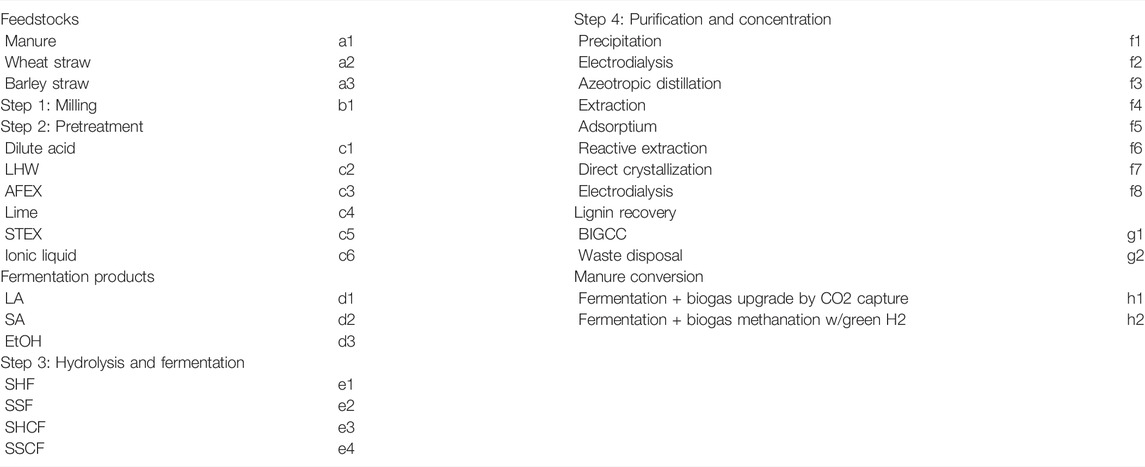
A Pareto front of solutions is obtained by applying the ϵ-constraint method, as presented in Section 3.2.2. The Pareto front is depicted in Figure 6; the corresponding production networks and data points are given in Table 2. The codes describing the different superstructure steps are reported in Table 1. The circles show the impact that changing the purification and concentration technologies (Step 4) has on the objective functions. Besides, it is worth noting that the impact of manure conversion is negligible when compared to changes in Step 4.

FIGURE 6

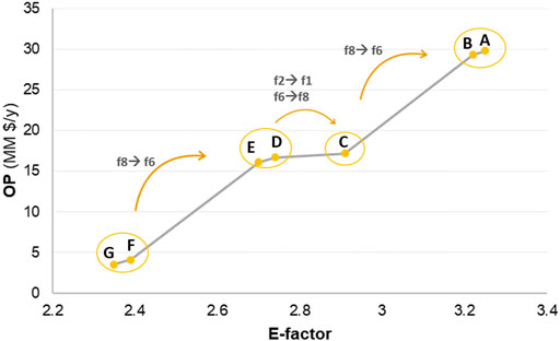
FIGURE 6. Pareto front of solutions: OP vs. E-factor. Extreme solutions: Solution A and Solution G.

TABLE 1

TABLE 1. Codes used to describe the solutions presented in Table 1 and Figure 6.

From Table 2 and Figure 6, the main differences among the solutions forming the Pareto front are the choice of technologies in Step 4 and manure conversion. However, the choice of manure conversion technologies does not impact the OP and E-factor as much as the selection of Step 4 (purification and concentration) technologies. The selection of different technologies in Step 4 is linked to the energy consumption and/or addition of solvents/chemicals. The most striking similarities are that (i) wheat straw is always selected as the main feedstock; (ii) dilute acid is invariably chosen as the pretreatment step; (iii) the selected technologies for Step 3 are consistent among all solutions; and (iv) lignin is consistently converted into electricity. Furthermore, a quick analysis of the extreme solutions shown in the Pareto front in Figure 6 is performed. Solution A, presented in Figure 7, represents the optimal OP (maximizes OP), and Solution G, depicted in Figure 8, stands for the optimal E-factor (minimizes waste production). Because both solutions have the same production targets, the main difference is the operating costs (raw materials/chemicals and feedstock). Overall, the following observations can be made by comparing solutions A and G.

TABLE 2

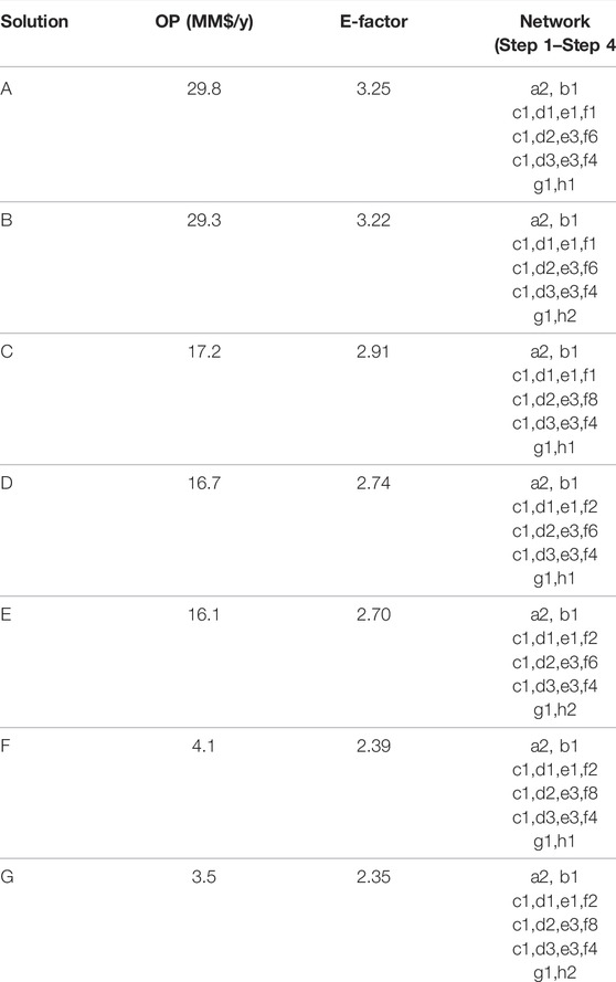
TABLE 2. Pareto of solutions as presented in Figure 6: OP, E-factor, and production network.

FIGURE 7

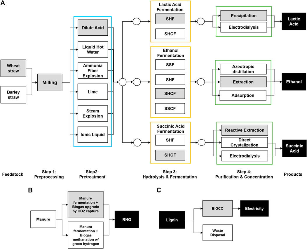
FIGURE 7. Solution A (maximizes OP): (A) LCF conversion, (B) manure conversion, and (C) lignin conversion. The grey shading represents the choice of feedstock and technologies.

FIGURE 8

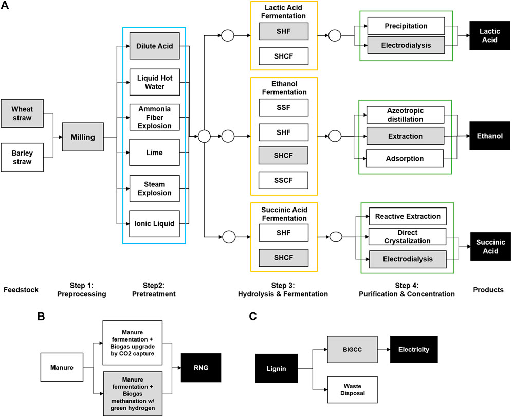
FIGURE 8. Solution G (minimizes E-factor): (A) LCF conversion, (B) manure conversion, and (C) lignin conversion. The grey shading represents the choice of feedstock and technologies.

Operating costs (OCs):

• As expected and presented in Figures 9, 10, the total OCs of Solution G are higher than Solution A (by approx. 15%).

• The OCs of Solution G are mainly due to Step’s 4 energy consumption (94.7%) in contrast to 44.2% for Solution A.

• The biggest part of the OC is the purification stage in both solutions: it represents 47.3% and 54.8% of the OC of Solutions A and G, respectively. This is followed by feedstock and enzyme-related costs.

• The total cost of utilities is divided into energy (e.g., cooling and heating) and raw materials costs (e.g., water and chemicals). The most impactful contributor to the cost of utilities in Solution A is the purchase of raw materials (57.7% of the cost of utilities), whereas the energy-related costs represent the biggest share of the cost of utilities in Solution G (78.7% of the cost of utilities).

• The total OCs of Solution G are higher than Solution A by approximately 15% (see Figures 9, 10);

• Solutions A and B have very similar OCs regarding all stages except for the purification and manure conversion steps (see Figure 6 and related discussion).

FIGURE 9

FIGURE 9. Solution A: operating cost by processing step.

FIGURE 10

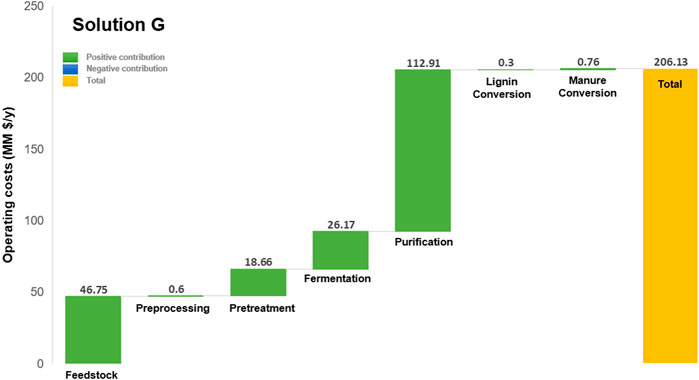
FIGURE 10. Solution G: operating cost by processing step.

Operating profit (OP):

• Solution A has eight times higher OP than Solution G (see Table 2).

• The contribution of heat and RNG/biogas production to the yearly revenue (and OCs) is rather small (depicted in Figure 11) due to the low production capacities set as the base case scenario. The production target was, as mentioned in Section 4, set based on existing biogas plants in Denmark, assuming that these plants are operating at optimal production capacities.

• Solution G has a higher possibility of improving OP if energy recycling technologies are implemented. The hypothesis is that the same percentage of energy can be recovered in Solutions A and G because the OC related to energy consumption in G is higher than in Solution A (absolute values). However, Solution A has a bigger profit margin, thus potentially allowing management to invest in approaches to improve the plant’s environmental and social burden (reduce E-factor).

FIGURE 11

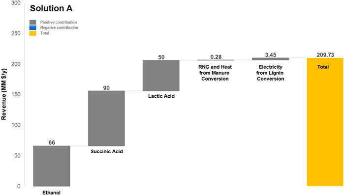
FIGURE 11. Solution A: contribution of the main products to the biorefinery’s revenue.

Assessment of OP by main product:The preceding discussion provides a summary of the biorefinery in its entirety and per processing stage. The analysis of the OP and OCs per product is detailed in this section. As previously mentioned, the model identifies the optimal network which leads to the target production capacities. Fixing the production capacity might force negative OP if all production pathways are not profitable (in this case, the model chooses the network that gives the least negative OP). Therefore, because the model does not give direct results on which products are the most optimal, it is important to analyze the contribution of each product to the OP, revenue, and OCs. Solution A is selected for this analysis, considering it has optimal OP.

• The OC per kg of main products (EtOH, SA, LA), as presented in Supplementary Table S10, is approximately 0.816 $/kg; the OP is 0.137 $/kg. The OC and OP per MWh of RNG produced are equal to 25$ and 9.5$, respectively. Note that this refers to the integrated biorefinery as a whole

• As shown in Figure 12, SA is the main contributor to the OC, followed by LA and EtOH.

• As observed, the production of LA is not advantageous in terms of economic feasibility (OC is higher than the OP; see Figure 13).

• The product ranking is, based on OP and EtOH, followed by SA and LA.

• Sensitivity analysis on product prices: the prices were updated to those reported in Gargalo et al. (2016). The new OP leads to a contrasting optimal solution, where LA is the most promising product, followed by SA and EtOH. This demonstrates that the economic feasibility is highly subject to input data (high model sensitivity and high data uncertainty)

• Performing uncertainty analysis would be very beneficial in increasing/improving the robustness of the model and corresponding results. This is part of future work.

FIGURE 12

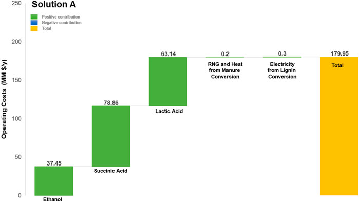
FIGURE 12. Solution A: contribution of the main products to the operating costs.

FIGURE 13

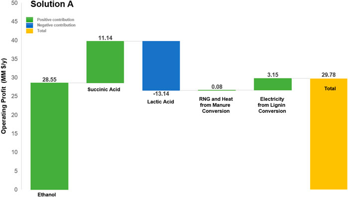
FIGURE 13. Solution A: contribution of the main products to the operating costs.

Furthermore, it is important to highlight that although the model developed in this work is extensive and comprehensive, it is based on available limited processing alternatives because research and implementation are ongoing. For example, Li et al. (2021) described the potential of using membrane technologies. Additionally, Step 3 was assumed to be pure culture fermentations; however, the review by Pinto et al. (2021) has documented that mixed cultures might bring some advantages. The superstructure does not include these alternatives due to the, so far, lack of maturity and data availability.

5 Conclusion and Future Perspectives

A novel model and multi-objective optimization tool, O2V, is proposed to identify design, planning, and operational decisions to develop and implement a second-generation integrated biorefinery to convert organic wastes into value-added products. It aims at being a holistic tool that integrates all pillars of sustainability. O2V model was built on an extensive superstructure of alternatives that include the process models and related data describing all steps concerning the treatment and conversion of biomass (structured database). A realistic case study has been selected on the potential development and implementation of an organic wastes integrated biorefinery in Denmark using LCF and manure. The products considered are ethanol, biogas, electricity, succinic acid, and lactic acid. Our strategy successfully identified the trade-off of solutions when optimizing economic feasibility and environmental and social impact for the potential implementation of this facility in Denmark. The optimal design and planning decisions have been identified for the extreme solutions (optimal OP and optimal E-factor). The major difference between these solutions is the technology chosen for purification and concentration steps. Of note is that the O2V model and optimization tool are extendable and adjustable in case of new data, or processing pathways become available, or both. Therefore, it has been shown that the O2V is a straightforward plug-and-play approach for early-stage design and assessment of organic wastes-based integrated biorefineries that aim to make the circular bio-economy a reality. Furthermore, future work includes integrating (i) the estimation of capital investment and (ii) uncertainty analysis into the O2V model to reach more robust solutions.

Step 1: Preprocessing

The variables and parameters linked to the pretreatment stage are follows:

• $Y_{S1}^{B_1}(b_1)$: binary variable. It represents the selection of feedstock b₁. If feedstock b₁ is chosen, variable $Y_{S1}^{B_1}(b_1)$ = 1 and = 0 otherwise.

• $Y_{S1}^{\mathit{Prep.}}(b_1,c)$: binary variable. It represents the selection of the preprocessing option c for feedstock b₁. If c is selected, variable $Y_{S1}^{\mathit{Prep.}}(b_1,c)$ = 1 and = 0 otherwise.

• $F_{S_1}(b_1,c)$: continuous variable. It represents the inflow of feedstock b₁ into preprocessing option c.

Step2: Pretreatment

The variables and parameters linked to the pretreatment stage are as follows:

• $F_{S_1\to S_2}(b_1,c,d)$: continuous variable. It is the amount of feedstock b₁ that underwent the preprocessing option c, which is subsequently sent to pretreatment option d.

• $Y_{S_2}(b_1,d)$: binary variable. It represents the selection of pretreatment option d for feedstock b₁. If pretreatment method d is selected for feedstock b₁, then $Y_{S_2}(b_1,d)$ = 1 and = 0 otherwise.

• $OU{T}_{S_1}$: variable. It represents the output milling particle size of the selected preprocessing option.

• $OU{T}_{S_1}^{\mathit{Preprocessing}}(c)$: parameter. It represents the output particle milling size given by preprocessing option c.

• $I{N}_{S_2}$: variable. It represents the maximum input particle size of the selected pretreatment option.

• $I{N}_{S_2}^{\mathit{Pretreatment}}(d)$: parameter. It represents the maximum input particle size of the selected pretreatment option d.

• $F_{S_2}(b_1,d,Cellulose)$: continuous variable. It is the flow of cellulose recovered from feedstock b₁ in the outlet solid phase of pretreatment option d.

• $F_{S_2}(b_1,d,Hemicellulose)$: continuous variable. It is the flow of hemicellulose recovered from feedstock b₁ in the outlet solid phase of pretreatment option d.

• $F_{S_2}(b_1,d,Ligni{n}_S)$: continuous variable. It represents the flow of lignin recovered from feedstock b₁ in the outlet solid phase of pretreatment option d.

• $F_{S_2}(b_1,d,Ligni{n}_L)$: continuous variable. It represents the amount of lignin recovered from feedstock b₁ in the outlet liquid phase of pretreatment option d.

• $F_{S_2}(b_1,d,Glucose)$: continuous variable. It represents the flow of glucose recovered from feedstock b₁ in the outlet liquid phase of pretreatment option d.

• $F_{S_2}(b_1,d,Xylose)$: continuous variable. It represents the flow of xylose recovered from feedstock b₁ in the outlet liquid phase of pretreatment option d.

• α^Cel (b₁): parameter. It represents the fraction of cellulose in feedstock b₁.

• α^HC(b₁): parameter. It represents the fraction of hemicellulose in feedstock b₁.

• α^Lig (b₁): parameter. It represents the fraction of lignin in feedstock b₁.

• ${\eta }_{S_2}(d,e)$: parameter. It represents the recovery factor of component e using pretreatment option d.

• $F_{S_2}^{BP}(b_1,d,f)$: continuous variable. It represents the flow of by-product f generated from feedstock b₁ which undergoes option d.

• ${\eta }_{S_2}^{BP}(d,f)$: parameter. It represents the amount of by-product f generated per kilo of feedstock undergoing pretreatment d.

• $F_{S_2}^{RM}(b_1,d,g)$: continuous variable. It represents the amount of utilities g consumed when feedstock b₁ undergoes option d.

• ${\eta }_{S_2}^{RM}(d,g)$: parameter. It represents the amount of utility g consumed per kilo of feedstock undergoing pretreatment d.

• $F_{S_2}^{\mathit{Liquid}}(b_1,d)$: continuous variable. It represents the total liquid flow recovered from feedstock b₁ undergoing option d.

• $F_{S_2}^{\mathit{Solid}}(b_1,d)$: continuous variable. It represents the total solid flow recovered from feedstock b₁ undergoing option d.

Step 3: Hydrolysis and fermentation

The variables and parameters linked to the bioconversion step are as follows:

• $F_{S_2}^{\mathit{Liquid}}(b_1,d)$: continuous variable. It represents the total liquid flow recovered from feedstock b₁ in pretreatment option d.

• $F_{S_2}^{\mathit{Solid}}(b_1,d)$: continuous variable. It represents the total solid flow recovered from feedstock b₁ in pretreatment option d.

• $F_{S_3}^{\mathit{Liquid}}(b_1,d,h,i)$: continuous variable. It represents the liquid flow recovered from feedstock b₁ in pretreatment option d sent to the Step 4 for the production of the main product h through fermentation technique i.

• $F_{S_3}^{\mathit{Solid}}(b_1,d,h,i)$: continuous variable. It represents the solid flow recovered from feedstock b₁ in pretreatment d sent to the fermentation section for the production of the main product h through fermentation technique i.

• ${\pi }_{S_3}(d,h,i)$: binary parametric matrix. It models the compatibility between pretreatment option d ∈ D, the production of the main product h ∈ H, and fermentation technique i ∈ I. If combination (d,h,i) is compatible, the parameter ${\pi }_{S_3}(d,h,i)$ = 1 and = 0 otherwise.

• $S{L}_{S_3}$: parameter. It represents the bioreactors target solid loading.

• $F_{S_3}^{\mathit{Water}}(b_1,h,i)$: continuous variable. It represents the flow of water added during sugar fermentation (from feedstock b₁) into main product h originating using the fermentation technique i.

• $Y_{S_3}^I(b_1,h,i)$: binary variable. It represents the selection of fermentation technique i for the production of the main product h from sugar fermentation (from feedstock b₁). If fermentation technique i is selected for the production of the main product h from sugars originating from feedstock b₁, $Y_{S_3}^I(b_1,h,i)$ = 1 and = 0 otherwise.

• $F_{S_3}^{\mathit{Xyl}}(b_1,d,h,i)$: continuous variable. It represents the xylose flow, produced from feedstock b₁ when the hemicellulose is hydrolysed, subsequently sent to the fermentation technique i for the production of the main product h.

• $F_{S_3}^{\mathit{Glu}}(b_1,d,h,i)$: continuous variable. It represents the flow of glucose (from feedstock b₁) by cellulose hydrolysis, which is subsequently sent for the production of the main product h through fermentation technique i.

• $F_{S_3}^{Xy{l}_L}(b_1,d,h,i)$: continuous variable. It represents the amount of xylose in the liquid outlet stream from pretreatment d sent to fermentation technique i for the production of the main product h.

• ${\eta }_{S_3}^{\mathit{Xyl}}(d)$: parameter. It represents the hemicellulose fraction converted into xylose by hydrolysis after pretreatment option d.

• ${\eta }_{S_3}^{\mathit{Glu}}(d)$: parameter. It represents the cellulose fraction converted into glucose by hydrolysis after pretreatment option d.

• $Y_{S_3,SH{F}_1}^J(b_1,h,j)$: binary variable. It represents the selection of fermentation strain j ∈ J for the production of the main product h through SHF from xylose in the liquid flow from pretreatment of feedstock b₁.

• $Y_{S_3,SH{F}_2}^J(b_1,h,j)$: binary variable. It represents the selection of fermentation strain j ∈ J for the production of the main product h through SHF from glucose and xylose in the solid flow from pretreatment of feedstock b₁.

• $F_{S_3}^{\mathit{Xyl-F}}(b_1,d,h,i,j)$: continuous variable. It represents the flow of xylose, from feedstock b₁ from hemicellulose hydrolysis, subsequently converted through fermentation technique i for the production of the main product h using fermentation strain j ∈ J.

• $F_{S_3}^{\mathit{Glu-F}}(b_1,d,h,i,j)$: continuous variable. It represents the flow of xylose, from feedstock b₁ from cellulose hydrolysis, subsequently converted through fermentation technique i for the production of the main product h using fermentation strain j ∈ J.

• $F_{S_3}^{Xy{l}_L-F}(b_1,d,h,i,j)$: continuous variable. It represents the flow of xylose recovered from the liquid stream, from feedstock b₁ from cellulose hydrolysis, subsequently converted through fermentation technique i for the production of the main product h using fermentation strain j ∈ J.

• ${\pi }_{S_3,S}^J(h,i,j)$: binary parametric matrix. It describes the compatibility among the production of the main product h ∈ H, the fermentation technique i ∈ I, and fermentation strain j ∈ J for the conversion of glucose and xylose produced through hydrolysis. If the combination (h,i,j) is compatible, ${\pi }_{S_3}(d,h,i)$ = 1 and = 0 otherwise.

• ${\pi }_{S_3,L}^J(h,i,j)$: binary parametric matrix. It describes the compatibility among the production of the main product h ∈ H, fermentation technique i ∈ I, and fermentation strain j ∈ J for the conversion of xylose from the liquid flow. If the combination (h,i,j) is compatible, ${\pi }_{S_3}(d,h,i)$ = 1 and = 0 otherwise.

• $F_{S_3}^{P-Xyl}(b_1,d,h,i,j)$: continuous variable. It represents the flow of the main product h produced from xylose (obtained from hemicellulose hydrolysis from feedstock b₁ that undergoes pretreatment d), using fermentation technique i and fermentation strain j ∈ J.

• $F_{S_3}^{P-Glu}(b_1,d,h,i,j)$: continuous variable. It represents the flow of the main product h from glucose conversion (obtained from cellulose hydrolysis from feedstock b₁, which undergoes pretreatment d), using fermentation technique i and fermentation strain j ∈ J.

• $F_{S_3}^{P-Xy{l}_L}(b_1,d,h,i,j)$: continuous variable. It represents the flow of the main product h from the conversion of xylose in the liquid stream (from pretreatment d of feedstock b₁), using the fermentation technique i and fermentation strain j ∈ J.

• ${\eta }_{S_3}^{P-Xyl}(d,j)$: parameter. It represents xylose’s conversion factor using strain j.

• ${\eta }_{S_3}^{P-Glu}(d,j)$: parameter. It represents the glucose’s conversion factor using the strain j.

• $F_{S_3}^{HC}(b_1,d,h,i)$: continuous variable. It represents the flow of hemicellulose (from the pretreatment option d of feedstock b₁) used for the production of the main product h through fermentation technique i.

• $F_{S_3}^{\mathit{Cel}}(b_1,d,h,i)$: continuous variable. It represents the flow of cellulose (from the pretreatment option d of feedstock b₁) used for the production of the main product h through fermentation technique i.

• $F_{S_3}^{HC-F}(b_1,d,h,i,j)$: continuous variable. It represents the flow of hemicellulose (from the pretreatment option d of feedstock b₁) used for the production of the main product h through fermentation technique i and fermentation strain j.

• $F_{S_3}^{\mathit{Cel-F}}(b_1,d,h,i,j)$: continuous variable. It represents the flow of cellulose (from the pretreatment option d of feedstock b₁) used for the production of the main product h through fermentation technique i and fermentation strain j.

• $Y_{S_3,SS{F}_1}^J(b_1,h,j)$: binary variable. It represents the selection of the fermentation strain j ∈ J for the conversion of xylose in the liquid outflow of pretreatment into the main product h using SSF.

• $Y_{S_3,SS{F}_2}^J(b_1,h,j)$: binary variable. It represents the selection of the fermentation strain j ∈ J for the conversion of glucose and xylose in the solid outflow of pretreatment into the main product h using SSF.

• $F_{S_3}^{P-Cel}(b_1,d,h,i,j)$: continuous variable. It represents the flow of the main product h obtained from the conversion of cellulose (recovered in pretreatment d of feedstock b₁) using fermentation technique i and fermentation strain j ∈ J.

• $F_{S_3}^{P-HC}(b_1,d,h,i,j)$: continuous variable. It represents the flow of the main product h obtained from the conversion of hemicellulose (recovered in pretreatment d of feedstock b₁) using fermentation technique i and fermentation strain j ∈ J.

• ${\eta }_{S_3}^{P-Cel}(d,j)$: parameter. It represents cellulose’s conversion factor using the strain j.

• ${\eta }_{S_3}^{P-HC}(d,j)$: parameter. It represents hemicellulose’s conversion factor using strain j.

• $F_{S_3}^{\mathit{Liquid-R}}(b_1,d,h,i)$: continuous variable. It represents the flow of liquid stream obtained before entering the fermentation reactor in co-fermentation configurations (to guarantee sufficient solid loading).

• $Y_{S_3,SHCF}^J(b_1,h,j)$: binary variable. It represents the selection of fermentation strain j ∈ J, for the conversion of fermentable sugars into the main product h using SHCF.

• $Y_{S_3,SSCF}^J(b_1,h,j)$: binary variable. It represents the selection of the fermentation strain j ∈ J for the conversion of fermentable sugars into the main product h using SHCF. This variable is indexed over sets B₁, H, and J.

• $F_{S_3}^P(h)$: continuous variable. It represents the total flow of product h produced during the fermentation stage.

Step 4: Purification and concentration

The variables and parameters linked to the purification and concentration step are as follows:

• $F_{S_4}(h,k)$: continuous variable. It represents the flow of the main product h sent to the purification and concentration process k.

• $Y_{S_4}(h,k)$: binary variable. It represents the selection of the purification and concentration process k for the main product h.

• $F_{S_4}^{P-R}(h,k)$: continuous variable. It represents the outflow of the main product h from the purification and concentration process k.

• ${\eta }_{S_4}(k)$: parameter. It represents the recovery factor of the purification and concentration process k. This parameter is indexed over the set K.

• $F_{S_4}^{P-Tot}(h)$: continuous variable. It represents the total outflow of the main product h from the purification and concentration stage.

• $F_{S_4}^{\mathit{Lignin-R}}$: continuous variable. It represents the flow of lignin recovered in Step 4 which is then converted into biogas.

• $Y_{S_4}^{\mathit{Lignin}}$: binary variable. It represents the selection of a lignin valorization step for the production of biogas.

• Manure conversion

The variables and parameters linked to the manure conversion are as follows:

• Y_Manure: binary variable. It represents the selection of manure conversion.

• $Y_{\mathit{Manure}}^L(l)$: binary variable. It represents the selection of the technology l ∈ L for manure conversion.

• F_Manure(l): continuous variable. It represents the inflow of manure into the processing option l ∈ L.

Data Availability Statement

The raw data supporting the conclusion of this article will be made available by the authors without undue reservation.

Author Contributions

All authors listed have made a substantial, direct, and intellectual contribution to the work and approved it for publication.

Conflict of Interest

The authors declare that the research was conducted in the absence of any commercial or financial relationships that could be construed as a potential conflict of interest.

Publisher’s Note

All claims expressed in this article are solely those of the authors and do not necessarily represent those of their affiliated organizations or those of the publisher, the editors, and the reviewers. Any product that may be evaluated in this article, or claim that may be made by its manufacturer, is not guaranteed or endorsed by the publisher.

Acknowledgments

The authors wish to acknowledge the financial support provided by the Novo Nordisk Foundation in the frame of the “Accelerated Innovation in Manufacturing Biologics” (AIMBio) project (Grant no. NNF19SA0035474).

Supplementary Material

The Supplementary Material for this article can be found online at: https://www.frontiersin.org/articles/10.3389/fceng.2022.837105/full#supplementary-material

References

Abdel-Rahman, M. A., Tashiro, Y., Zendo, T., Sakai, K., and Sonomoto, K. (2015). Enterococcus Faecium Qu 50: a Novel Thermophilic Lactic Acid Bacterium for High-Yield L-Lactic Acid Production from Xylose. FEMS Microbiol. Lett. 362, 1–7. doi:10.1093/femsle/fnu030

CrossRef Full Text | Google Scholar

Aden, A., Ruth, M., Ibsen, K., Jechura, J., Neeves, K., Sheehan, J., et al. (2002). Golden, CO.(US). Lignocellulosic Biomass to Ethanol Process Design and Economics Utilizing Co-current Dilute Acid Prehydrolysis and Enzymatic Hydrolysis for Corn StoverTech. Rep. Natl. Renew. Energy Lab. doi:10.2172/15001119

CrossRef Full Text | Google Scholar

Alibaba (2020a). Chloride. Available at: https://www.alibaba.com/product-detail/Ferric-Chloride-Chloride-Ferric-Chloride-Price_62095133477.html?spm=a2700.7724857.normal_offer.d_image.5466156870qa88&s=p.

Google Scholar

Alibaba (2020b). Oxide. Available at: https://www.alibaba.com/product-detail/Magnesium-Oxide-Industry-Magnesium-Oxide-Producers_62058751813.html?spm=a2700.galleryofferlist.normal_offer.d_title.3eb77b05GuAeXi&s=p.

Google Scholar

Alibaba (2020c). Water Treatment Chemicals. Available at: https://www.alibaba.com/product-detail/Calcium-Hydroxide-Factory-Direct-White-Powder_1600227110322.html?spm=a2700.7724857.normal_offer.d_image.5ed9229eUO5hqA&s=p.

Google Scholar

Álvarez del Castillo-Romo, A., Morales-Rodriguez, R., and Román-Martínez, A. (2018). Multiobjective Optimization for the Socio-Eco-Efficient Conversion of Lignocellulosic Biomass to Biofuels and Bioproducts. Clean. Techn Environ. Policy 20, 603–620. doi:10.1007/s10098-018-1490-x

CrossRef Full Text | Google Scholar

Aristizábal‐Marulanda, V., and Cardona Alzate, C. A. (2019). Methods for Designing and Assessing Biorefineries: Review. Biofuels, Bioprod. Bioref. 13, 789–808. doi:10.1002/bbb.1961

CrossRef Full Text | Google Scholar

Balan, V., Sousa, L. d. C., Chundawat, S. P. S., Marshall, D., Sharma, L. N., Chambliss, C. K., et al. (2009). Enzymatic Digestibility and Pretreatment Degradation Products of Afex-Treated Hardwoods (Populus Nigra). Biotechnol. Prog. 25, 365–375. doi:10.1002/btpr.160

PubMed Abstract | CrossRef Full Text | Google Scholar

Bao, B., Ng, D. K. S., Tay, D. H. S., Jiménez-Gutiérrez, A., and El-Halwagi, M. M. (2011). A Shortcut Method for the Preliminary Synthesis of Process-Technology Pathways: An Optimization Approach and Application for the Conceptual Design of Integrated Biorefineries. Comput. Chem. Eng. 35, 1374–1383. doi:10.1016/j.compchemeng.2011.04.013

CrossRef Full Text | Google Scholar

Bastidas, P. A., Gil, I. D., and Rodríguez, G. (2010). “Comparison of the Main Ethanol Dehydration Technologies through Process Simulation,” in European Symposium on Computer Aided Process Engineering, 20th.

Google Scholar

Belletante, S., Montastruc, L., Meyer, M., Hermansyah, H., and Negny, S. (2020). Multiproduct Biorefinery Optimal Design: Application to the Acetone-Butanol-Ethanol System. Oil Gas. Sci. Technol. - Rev. IFP Energies Nouv. 75, 9. doi:10.2516/ogst/2020002

CrossRef Full Text | Google Scholar

Bertran, M.-O., Frauzem, R., Sanchez-Arcilla, A.-S., Zhang, L., Woodley, J. M., and Gani, R. (2017). A Generic Methodology for Processing Route Synthesis and Design Based on Superstructure Optimization. Comput. Chem. Eng. 106, 892–910. doi:10.1016/j.compchemeng.2017.01.030

CrossRef Full Text | Google Scholar

Bozell, J. J., and Petersen, G. R. (2010). Technology Development for the Production of Biobased Products from Biorefinery Carbohydrates-The US Department of Energy's "Top 10" Revisited. Green Chem. 12, 539–554. doi:10.1039/b922014c

CrossRef Full Text | Google Scholar

Cheali, P., Gernaey, K. V., and Sin, G. (2014). Toward a Computer-Aided Synthesis and Design of Biorefinery Networks: Data Collection and Management Using a Generic Modeling Approach. ACS Sustain. Chem. Eng. 2, 19–29. doi:10.1021/sc400179f

CrossRef Full Text | Google Scholar

Chemmangattuvalappil, N. G., and Ng, D. K. S. (2013). Systematic Methodology for Optimal Product Design in an Integrated Biorefinery. Comput. Aided Chem. Eng. 32, 91–96. doi:10.1016/b978-0-444-63234-0.50016-6

CrossRef Full Text | Google Scholar

Chemmangattuvalappil, N. G., Ng, D. K. S., Ng, L. Y., Ooi, J., Chong, J. W., and Eden, M. R. (2020). A Review of Process Systems Engineering (Pse) Tools for the Design of Ionic Liquids and Integrated Biorefineries. Processes 8, 1678–1708. doi:10.3390/pr8121678

CrossRef Full Text | Google Scholar

Chen, Q., and Grossmann, I. (2019a). Modern Modeling Paradigms Using Generalized Disjunctive Programming. Processes 7, 839. doi:10.3390/pr7110839

CrossRef Full Text | Google Scholar

Chen, Q., and Grossmann, I. (2019b). Modern Modeling Paradigms Using Generalized Disjunctive Programming. Processes 7, 839. doi:10.3390/pr7110839

CrossRef Full Text | Google Scholar

Chen, Q., Johnson, E. S., Siirola, J. D., and Grossmann, I. E. (2018a). Pyomo.GDP: Disjunctive Models in Python. Comput. Aided Chem. Eng. 44, 889–894. doi:10.1016/b978-0-444-64241-7.50143-9

CrossRef Full Text | Google Scholar

Chen, Q., Johnson, E. S., Siirola, J. D., and Grossmann, I. E. (2018b). “Pyomo.gdp: Disjunctive Models in python,”. 13th International Symposium on Process Systems Engineering (PSE 2018). Editors M. R. Eden, M. G. Ierapetritou, and G. P. Towler (ElsevierComputer Aided Chemical Engineering), 44, 889–894. 889–894. doi:10.1016/B978-0-444-64241-7.50143-9

CrossRef Full Text | Google Scholar

Conde-Mejía, C., Jiménez-Gutiérrez, A., and El-Halwagi, M. M. (2013). Assessment of Combinations between Pretreatment and Conversion Configurations for Bioethanol Production. ACS Sustain. Chem. Eng. 1, 956–965. doi:10.1021/sc4000384

CrossRef Full Text | Google Scholar

da Costa Sousa, L., Chundawat, S. P., Balan, V., and Dale, B. E. (2009). 'Cradle-to-grave' Assessment of Existing Lignocellulose Pretreatment Technologies. Curr. Opin. Biotechnol. 20, 339–347. doi:10.1016/j.copbio.2009.05.003

PubMed Abstract | CrossRef Full Text | Google Scholar

Denmark, S. (2020a). Livestock Combination by Unit, Time and Type. Available at: https://www.statbank.dk/statbank5a/selectvarval/define.asp?PLanguage=1&subword=tabsel&MainTable=KOMB07&PXSId=147398&tablestyle=&ST=SD&buttons=0.

Google Scholar

Denmark, S. (2020b). Statbank denmark. Available at: https://www.statbank.dk/10474.

Google Scholar

Di Lorenzo, M. L., and Androsch, R. (2018). Synthesis, Structure and Properties of Poly (Lactic Acid). Springer.

Google Scholar

Dutta, A., Dowe, N., Ibsen, K. N., Schell, D. J., and Aden, A. (2010). An Economic Comparison of Different Fermentation Configurations to Convert Corn Stover to Ethanol Using Z. Mobilis and saccharomyces. Biotechnol. Prog. 26, 64–72. doi:10.1002/btpr.311

PubMed Abstract | CrossRef Full Text | Google Scholar

ECHEMI (2020a). Ammonia Market Price Analysis. Available at: https://www.echemi.com/productsInformation/pid_Rock19411-ammonia.html.

Google Scholar

ECHEMI (2020b). Ethylene Glycol (Eg) Market Price Analysis. Available at: https://www.echemi.com/productsInformation/pid_Seven2471-ethylene-glycol-eg.html.

Google Scholar

Elyasi, S. N., Rafiee, S., Mohtasebi, S. S., Tsapekos, P., Angelidaki, I., Liu, H., et al. (2021). An Integer Superstructure Model to Find a Sustainable Biorefinery Platform for Valorizing Household Waste to Bioenergy, Microbial Protein, and Biochemicals. J. Clean. Prod. 278, 123986. doi:10.1016/j.jclepro.2020.123986

CrossRef Full Text | Google Scholar

Eurostat (2020b). Gas prices for household consumers - bi-annual data. from 2007 onwards. Available at: https://ec.europa.eu/eurostat/databrowser/view/nrg_pc_202/default/table?lang=en.

Google Scholar

Eurostat (2020a). Electricity Price Statistics. https://ec.europa.eu/eurostat/statistics-explained/index.php?title=Electricity_price_statistics#Electricity_prices_for_non-household_consumers.

Google Scholar

Ferone, M., Raganati, F., Ercole, A., Olivieri, G., Salatino, P., and Marzocchella, A. (2018). Continuous Succinic Acid Fermentation by Actinobacillus Succinogenes in a Packed-Bed Biofilm Reactor. Biotechnol. Biofuels 11, 138–149. doi:10.1186/s13068-018-1143-7

PubMed Abstract | CrossRef Full Text | Google Scholar

Furlan, F. F., Costa, C. B. B., Fonseca, G. d. C., Soares, R. d. P., Secchi, A. R., Cruz, A. J. G. d., et al. (2012). Assessing the Production of First and Second Generation Bioethanol from Sugarcane through the Integration of Global Optimization and Process Detailed Modeling. Comput. Chem. Eng. 43, 1–9. doi:10.1016/j.compchemeng.2012.04.002

CrossRef Full Text | Google Scholar

Gabriel, K. J., and El-Halwagi, M. M. (2013). Modeling and Optimization of a Bioethanol Production Facility. Clean. Techn Environ. Policy 15, 931–944. doi:10.1007/s10098-013-0584-8

CrossRef Full Text | Google Scholar

Galanopoulos, C., Giuliano, A., Barletta, D., and Zondervan, E. (2019). An Optimization Model for a Biorefinery System Based on Process Design and Logistics. Comput. Aided Chem. Eng. 46, 265–270. doi:10.1016/B978-0-12-818634-3.50045-X

CrossRef Full Text | Google Scholar

Gargalo, C. L., Carvalho, A., Gernaey, K. V., and Sin, G. (2017). Supply Chain Optimization of Integrated Glycerol Biorefinery: Glythink Model Development and Application. Ind. Eng. Chem. Res. 56, 6711–6727. doi:10.1021/acs.iecr.7b00908

CrossRef Full Text | Google Scholar

Gargalo, C. L., Cheali, P., Posada, J. A., Gernaey, K. V., and Sin, G. (2016). Economic Risk Assessment of Early Stage Designs for Glycerol Valorization in Biorefinery Concepts. Ind. Eng. Chem. Res. 55, 6801–6814. doi:10.1021/acs.iecr.5b04593

CrossRef Full Text | Google Scholar

Gargalo, C. L., Jones, M. N., Udugama, I., Mansouri, S. S., Krühne, U., Gernaey, K. V., et al. (2020). Towards the Development of Digital Twins for the Bio-Manufacturing Industry. Adv. Biochem. Engineering/biotechnology 176, 1–34. doi:10.1007/10_2020_142

CrossRef Full Text | Google Scholar

Garlock, R. J., Balan, V., Dale, B. E., Ramesh Pallapolu, V., Lee, Y. Y., Kim, Y., et al. (2011). Comparative Material Balances Around Pretreatment Technologies for the Conversion of Switchgrass to Soluble Sugars. Bioresour. Technol. 102, 11063–11071. doi:10.1016/j.biortech.2011.04.002

PubMed Abstract | CrossRef Full Text | Google Scholar

Geraili, A., and Romagnoli, J. A. (2015). A Multiobjective Optimization Framework for Design of Integrated Biorefineries under Uncertainty. AIChE J. 61, 3208–3222. doi:10.1002/aic.14849

CrossRef Full Text | Google Scholar

Giarola, S., Zamboni, A., and Bezzo, F. (2011). Spatially Explicit Multi-Objective Optimisation for Design and Planning of Hybrid First and Second Generation Biorefineries. Comput. Chem. Eng. 35, 1782–1797. doi:10.1016/j.compchemeng.2011.01.020

CrossRef Full Text | Google Scholar

Gil, I. D., Uyazán, A. M., Aguilar, J. L., Rodríguez, G., and Caicedo, L. A. (2008). Separation of Ethanol and Water by Extractive Distillation with Salt and Solvent as Entrainer: Process Simulation. Braz. J. Chem. Eng. 25, 207–215. doi:10.1590/s0104-66322008000100021

CrossRef Full Text | Google Scholar

Giuliano, A., Cerulli, R., Poletto, M., Raiconi, G., and Barletta, D. (2016). Process Pathways Optimization for a Lignocellulosic Biorefinery Producing Levulinic Acid, Succinic Acid, and Ethanol. Ind. Eng. Chem. Res. 55, 10699–10717. doi:10.1021/acs.iecr.6b01454

CrossRef Full Text | Google Scholar

Gomez, L. D., Steele‐King, C. G., and McQueen‐Mason, S. J. (2008). Sustainable Liquid Biofuels from Biomass: the Writing's on the Walls. New Phytol. 178, 473–485. doi:10.1111/j.1469-8137.2008.02422.x

PubMed Abstract | CrossRef Full Text | Google Scholar

Gong, J., and You, F. (2014). Optimal Design and Synthesis of Algal Biorefinery Processes for Biological Carbon Sequestration and Utilization with Zero Direct Greenhouse Gas Emissions: Minlp Model and Global Optimization Algorithm. Ind. Eng. Chem. Res. 53, 1563–1579. doi:10.1021/ie403459m

CrossRef Full Text | Google Scholar

González-García, S., Iribarren, D., Susmozas, A., Dufour, J., and Murphy, R. J. (2012). Life Cycle Assessment of Two Alternative Bioenergy Systems Involving Salix Spp. Biomass: Bioethanol Production and Power Generation. Appl. Energy 95, 111–122. doi:10.1016/j.apenergy.2012.02.022

CrossRef Full Text | Google Scholar

Grossmann, I. E., and Trespalacios, F. (2013). Systematic Modeling of Discrete-Continuous Optimization Models through Generalized Disjunctive Programming. AIChE J. 59, 3276–3295. doi:10.1002/aic.14088

CrossRef Full Text | Google Scholar

Hernández-Calderón, O. M., Ponce-Ortega, J. M., Ortiz-Del-Castillo, J. R., Cervantes-Gaxiola, M. E., Milán-Carrillo, J., Serna-González, M., et al. (2016). Optimal Design of Distributed Algae-Based Biorefineries Using Co2 Emissions from Multiple Industrial Plants. Ind. Eng. Chem. Res. 55, 2345–2358. doi:10.1021/acs.iecr.5b01684

CrossRef Full Text | Google Scholar

Hills, D. J., and Roberts, D. W. (1981). Anaerobic Digestion of Dairy Manure and Field Crop Residues. Agric. Wastes 3, 179–189. doi:10.1016/0141-4607(81)90026-3

CrossRef Full Text | Google Scholar

Humbird, D., Davis, R., Tao, L., Kinchin, C., Hsu, D., Aden, A., et al. (2011).Process Design and Economics for Biochemical Conversion of Lignocellulosic Biomass to Ethanol: Dilute-Acid Pretreatment and Enzymatic Hydrolysis of Corn Stover. Tech. Rep. Natl. Renew. Energy Lab.(NREL). doi:10.2172/1013269

CrossRef Full Text | Google Scholar

Isikgor, F. H., and Becer, C. R. (2015). Lignocellulosic Biomass: a Sustainable Platform for the Production of Bio-Based Chemicals and Polymers. Polym. Chem. 6, 4497–4559. doi:10.1039/c5py00263j

CrossRef Full Text | Google Scholar

Kampman, B., Leguijt, C., Scholten, T., Tallat-Kelpsaite, J., Brückmann, R., Maroulis, G., et al. (2017). Optimal Use of Biogas from Waste Streams: An Assessment of the Potential of Biogas from Digestion in the Eu beyond 2020.

Google Scholar

Kelloway, A., and Daoutidis, P. (2014). Process Synthesis of Biorefineries: Optimization of Biomass Conversion to Fuels and Chemicals. Ind. Eng. Chem. Res. 53, 5261–5273. doi:10.1021/ie4018572

CrossRef Full Text | Google Scholar

Khoshnevisan, B., Duan, N., Tsapekos, P., Awasthi, M. K., Liu, Z., Mohammadi, A., et al. (2021). A Critical Review on Livestock Manure Biorefinery Technologies: Sustainability, Challenges, and Future Perspectives. Renew. Sustain. Energy Rev. 135, 110033. doi:10.1016/j.rser.2020.110033

CrossRef Full Text | Google Scholar

Komesu, A., Maciel, M. R. W., and Maciel Filho, R. (2017). Separation and Purification Technologies for Lactic Acid–A Brief Review. BioResources 12, 6885–6901. doi:10.15376/biores.12.3.6885-6901

CrossRef Full Text | Google Scholar

Kühner, S. (2013). Feedstock Costs. Deliverable D1 1.

Google Scholar

Kumar, P., Barrett, D. M., Delwiche, M. J., and Stroeve, P. (2009). Methods for Pretreatment of Lignocellulosic Biomass for Efficient Hydrolysis and Biofuel Production. Ind. Eng. Chem. Res. 48, 3713–3729. doi:10.1021/ie801542g

CrossRef Full Text | Google Scholar

Lee, A., Ghouse, J. H., Chen, Q., Eslick, J. C., Siirola, J. D., Grossman, I. E., et al. (2018). “A Flexible Framework and Model Library for Process Simulation, Optimization and Control,” in 13th International Symposium on Process Systems Engineering (PSE 2018). Editors M. R. Eden, M. G. Ierapetritou, and G. P. Towler (Elsevier), 44, 937–942. of Computer Aided Chemical Engineering. doi:10.1016/B978-0-444-64241-7.50151-8

CrossRef Full Text | Google Scholar

Lee, H. (2015). Development of lactic and succinic acid biorefinery configurations for integration into a thermomechanical pulp mill. Ph.D. thesis, École Polytechnique de Montréal.

Google Scholar

Li, C., Tanjore, D., He, W., Wong, J., Gardner, J. L., Sale, K. L., et al. (2013a). Scale-up and Evaluation of High Solid Ionic Liquid Pretreatment and Enzymatic Hydrolysis of Switchgrass. Biotechnol. Biofuels 6, 154–167. doi:10.1186/1754-6834-6-154

PubMed Abstract | CrossRef Full Text | Google Scholar

Li, H. Q., Li, C. L., Sang, T., and Xu, J. (2013b). Pretreatment on Miscanthus Lutarioriparious by Liquid Hot Water for Efficient Ethanol Production. Biotechnol. Biofuels 6, 76–10. doi:10.1186/1754-6834-6-76

PubMed Abstract | CrossRef Full Text | Google Scholar

Li, Y., Bhagwat, S. S., Cortés-Peña, Y. R., Ki, D., Rao, C. V., Jin, Y.-S., et al. (2021). Sustainable Lactic Acid Production from Lignocellulosic Biomass. ACS Sustain. Chem. Eng. 9, 1341–1351. doi:10.1021/acssuschemeng.0c08055

CrossRef Full Text | Google Scholar

Losinger, W. C., and Sampath, R. K. (2000). Economies of Scale in the Production of Swine Manure. Arq. Bras. Med. Vet. Zootec. 52, 285–294. doi:10.1590/s0102-09352000000300019

CrossRef Full Text | Google Scholar

Made-in-China (2020a). Cyclohexane. Available at: https://sinowin.en.made-in-china.com/product/rSbxomnvYsUl/China-CAS-110-82-7-High-Quality-Industrial-Liquid-Cyclohexane.html.

Google Scholar

Made-in-China (2020b). Refractory Forsterite Calcined Olivine Sand for Foundry. Available at: https://ditaichem.en.made-in-china.com/product/fvJQwCHxHNWY/China-Refractory-Forsterite-Calcined-Olivine-Sand-for-Foundry.html.

Google Scholar

Madenoor Ramapriya, G., Won, W., and Maravelias, C. T. (2018). A Superstructure Optimization Approach for Process Synthesis under Complex Reaction Networks. Chem. Eng. Res. Des. 137, 589–608. doi:10.1016/j.cherd.2018.07.015

CrossRef Full Text | Google Scholar

Mani, S., Tabil, L. G., and Sokhansanj, S. (2004). Grinding Performance and Physical Properties of Wheat and Barley Straws, Corn Stover and Switchgrass. Biomass bioenergy 27, 339–352. doi:10.1016/j.biombioe.2004.03.007

CrossRef Full Text | Google Scholar

Martin, C., Marcet, M., and Thomsen, A. B. (2008). Comparison between Wet Oxidation and Steam Explosion as Pretreatment Methods for Enzymatic Hydrolysis of Sugarcane Bagasse. BioResources 3, 670–683.

Google Scholar

Mencarelli, L., Chen, Q., Pagot, A., and Grossmann, I. E. (2020). A Review on Superstructure Optimization Approaches in Process System Engineering. Comput. Chem. Eng. 136, 106808. doi:10.1016/j.compchemeng.2020.106808

CrossRef Full Text | Google Scholar

Methanex (2021). Methanex Posts Regional Contract Methanol Prices for North america, Europe and Asia. Available at: https://www.methanex.com/our-business/pricing.

Google Scholar

Ng, R. T. L., Fasahati, P., Huang, K., and Maravelias, C. T. (2019). Utilizing Stillage in the Biorefinery: Economic, Technological and Energetic Analysis. Appl. Energy 241, 491–503. doi:10.1016/j.apenergy.2019.03.020

CrossRef Full Text | Google Scholar

Ng, R. T. L., Tay, D. H. S., and Ng, D. K. S. (2012). Simultaneous Process Synthesis, Heat and Power Integration in a Sustainable Integrated Biorefinery. Energy fuels. 26, 7316–7330. doi:10.1021/ef301283c

CrossRef Full Text | Google Scholar

Nilsson, D., Bentsen, N. S., Larsen, S., and Stupak, I. (2016). Agricultural Residues for Energy in sweden and denmark – Differences and Commonalities.

Google Scholar

Panoutsou, C., and Singh, A. (2020). Denmark Roadmap for Lignocellulosic Biomass and Relevant Policies for a Bio-Based Economy in 2030.

Google Scholar

Pham, V., and El-Halwagi, M. (2012). Process Synthesis and Optimization of Biorefinery Configurations. AIChE J. 58, 1212–1221. doi:10.1002/aic.12640

CrossRef Full Text | Google Scholar

PharmaCompass (2020a). Lactic Acid. Available at: https://www.pharmacompass.com/price/lactic-acid.

Google Scholar

PharmaCompass (2020b). Monoethanolamine. Available at: https://www.pharmacompass.com/price/monoethanolamine.

Google Scholar

Pinto, T., Flores-Alsina, X., Gernaey, K. V., and Junicke, H. (2021). Alone or Together? a Review on Pure and Mixed Microbial Cultures for Butanol Production. Renew. Sustain. Energy Rev. 147, 111244. doi:10.1016/j.rser.2021.111244

CrossRef Full Text | Google Scholar

Ponce-Ortega, J. M., Pham, V., El-Halwagi, M. M., and El-Baz, A. A. (2012a). A Disjunctive Programming Formulation for the Optimal Design of Biorefinery Configurations. Ind. Eng. Chem. Res. 51, 3381–3400. doi:10.1021/ie201599m

CrossRef Full Text | Google Scholar

Ponce-Ortega, J. M., Pham, V., El-Halwagi, M. M., and El-Baz, A. A. (2012b). A Disjunctive Programming Formulation for the Optimal Design of Biorefinery Configurations. Ind. Eng. Chem. Res. 51, 3381–3400. doi:10.1021/ie201599m

CrossRef Full Text | Google Scholar

Proinic (2021). Emim Oac. Available at: https://proionic.com/bestseller/EMIM-OAc.php.

Google Scholar

Raftery, J. P., and Karim, M. N. (2014).A Methodology for the Optimization of Bioethanol Production via Biochemical Pathways. Comput. Aided Chem. Eng. 34, 597–602. doi:10.1016/b978-0-444-63433-7.50084-5

CrossRef Full Text | Google Scholar

Restrepo-Flórez, J. M., and Maravelias, C. T. (2020). Advanced Fuels from Ethanol–A Superstructure Optimization Approach. Energy & Environ. Sci. 14.

Google Scholar

Rizwan, M., Lee, J. H., and Gani, R. (2015). Optimal Design of Microalgae-Based Biorefinery: Economics, Opportunities and Challenges. Appl. Energy 150, 69–79. doi:10.1016/j.apenergy.2015.04.018

CrossRef Full Text | Google Scholar

Santibañez-Aguilar, J. E., González-Campos, J. B., Ponce-Ortega, J. M., Serna-González, M., and El-Halwagi, M. M. (2011). Optimal Planning of a Biomass Conversion System Considering Economic and Environmental Aspects. Ind. Eng. Chem. Res. 50, 8558–8570. doi:10.1021/ie102195g

CrossRef Full Text | Google Scholar

Sheldon, R. A. (2017). The E Factor 25 Years on: the Rise of Green Chemistry and Sustainability. Green Chem. 19, 18–43. doi:10.1039/c6gc02157c

CrossRef Full Text | Google Scholar

Skorek-Osikowska, A., Martín-Gamboa, M., and Dufour, J. (2020). Thermodynamic, Economic and Environmental Assessment of Renewable Natural Gas Production Systems. Energy Convers. Manag. X 7, 100046. doi:10.1016/j.ecmx.2020.100046

CrossRef Full Text | Google Scholar

Støckler, M., Berman, D., Jensen, T. Y. H. W., and Harder, B. (2020). Biogas Production: Insights and Experiences from the Danish Biogas Sector. Available at: https://biogasclean.com/wp-content/uploads/2021/02/biogas-in-denmark-june-2020.pdf.

Google Scholar

Struhs, E., Mirkouei, A., You, Y., and Mohajeri, A. (2020). Techno-economic and Environmental Assessments for Nutrient-Rich Biochar Production from Cattle Manure: A Case Study in idaho, usa. Appl. Energy 279, 115782. doi:10.1016/j.apenergy.2020.115782

CrossRef Full Text | Google Scholar

Sun, R., Lawther, J. M., and Banks, W. B. (1996). Fractional and Structural Characterization of Wheat Straw Hemicelluloses. Carbohydr. Polym. 29, 325–331. doi:10.1016/s0144-8617(96)00018-5

CrossRef Full Text | Google Scholar

Svensson, E., Eriksson, K., and Wik, T. (2015). Reasons to Apply Operability Analysis in the Design of Integrated Biorefineries. Biofuels, Bioprod. Bioref. 9, 147–157. doi:10.1002/bbb.1530

CrossRef Full Text | Google Scholar

Tey, T. O., Chen, S., Cheong, Z. X., Choong, A. S. X., Ng, L. Y., and Chemmangattuvalappil, N. G. (2021). Synthesis of a Sustainable Integrated Biorefinery to Produce Value-Added Chemicals from Palm-Based Biomass via Mathematical Optimisation. Sustain. Prod. Consum. 26, 288–315. doi:10.1016/j.spc.2020.10.012

CrossRef Full Text | Google Scholar

UnitedNations (2019). Circular Economy Crucial for Paris Climate Goals. 2021–2111.

Google Scholar

Vaswani, S. (2010). Bio-based Succinic Acid. SRI Consult. Rev.

Google Scholar

Vecchietti, A., Lee, S., and Grossmann, I. E. (2003). Modeling of Discrete/continuous Optimization Problems: Characterization and Formulation of Disjunctions and Their Relaxations. Comput. Chem. Eng. 27, 433–448. doi:10.1016/s0098-1354(02)00220-x

CrossRef Full Text | Google Scholar

Venkata Mohan, S., Dahiya, S., Amulya, K., Katakojwala, R., and Vanitha, T. K. (2019). Can Circular Bioeconomy Be Fueled by Waste Biorefineries - A Closer Look. Bioresour. Technol. Rep. 7, 100277. doi:10.1016/j.biteb.2019.100277

CrossRef Full Text | Google Scholar

Vikash, P. V., and Shastri, Y. (2019). Conceptual Design of a Lignocellulosic Biorefinery and its Supply Chain for Ethanol Production in india. Comput. Chem. Eng. 121, 696–721. doi:10.1016/j.compchemeng.2018.11.021

CrossRef Full Text | Google Scholar

Villadsen, J. (2013). Industrial Production of Succinic Acid – a Stepwise Approach. GIM.

Google Scholar

Wang, B., Gebreslassie, B. H., and You, F. (2013). Sustainable Design and Synthesis of Hydrocarbon Biorefinery via Gasification Pathway: Integrated Life Cycle Assessment and Technoeconomic Analysis with Multiobjective Superstructure Optimization. Comput. Chem. Eng. 52, 55–76. doi:10.1016/j.compchemeng.2012.12.008

CrossRef Full Text | Google Scholar

You, F., Tao, L., Graziano, D. J., and Snyder, S. W. (2012). Optimal Design of Sustainable Cellulosic Biofuel Supply Chains: Multiobjective Optimization Coupled with Life Cycle Assessment and Input-Output Analysis. AIChE J. 58, 1157–1180. doi:10.1002/aic.12637

CrossRef Full Text | Google Scholar

Zhang, Q., Martín, M., and Grossmann, I. E. (2019). Integrated Design and Operation of Renewables-Based Fuels and Power Production Networks. Comput. Chem. Eng. 122, 80–92. doi:10.1016/j.compchemeng.2018.06.018

CrossRef Full Text | Google Scholar

Zondervan, E., Nawaz, M., de Haan, A. B., Woodley, J. M., and Gani, R. (2011a). Optimal Design of a Multi-Product Biorefinery System. Comput. Chem. Eng. 35, 1752–1766. doi:10.1016/j.compchemeng.2011.01.042

CrossRef Full Text | Google Scholar

Zondervan, E., Nawaz, M., de Haan, A. B., Woodley, J. M., and Gani, R. (2011b). Optimal Design of a Multi-Product Biorefinery System. Comput. Chem. Eng. 35, 1752–1766. doi:10.1016/j.compchemeng.2011.01.042

CrossRef Full Text | Google Scholar

Nomenclature

Glossary

SA succinic acid

LA lactic acid

EtOH ethanol

LCF lignocellulosic feedstock

DM dimethyl ether

EG ethylene glycol

DC dimethyl carbonate

1,4-BDO 1,4-butanediol

GWP global warming potential

NPV net present value

MINLP mixed-integer non-linear programming

GDP generalized disjunctive programming

SHF separate hydrolysis and fermentation

SHCF separate hydrolysis and co-fermentation

SSF simultaneous saccharification and fermentation

SSCF simultaneous saccharification and co-fermentation

RNG renewable natural gas-biogas

BIGCC biomass integrated gasification combined cycle.

Indices

b feedstocks

c preprocessing options (Step 1)

d pretreatment options (Step 2)

e components

f by-products

g utilities

h hydrolysis and fermentation options (Step 3)

i fermentation techniques (e.g., SSF, SSCF)

k purification and concentration options

l manure conversion options.

Sets

B set of all feedstocks b

C set of all preprocessing options c

D set of all pretreatment options c

E set of all components e

F set of all by-products f

G set of all utilities g

H set of all Step 3 options h

I set of all fermentation techniques i

K set of all purification and concentration options k

L set of all manure conversion options.