Speeding up deep neural architecture search for wearable activity recognition with early prediction of converged performance

1. Introduction

Designing a deep neural network (DNN) for human activity recognition (HAR) (Wang et al., 2019) requires making decisions about many architectural hyperparameters, including layer types, sizes, numbers of, and connections between layers. Due to the extremely large space of neural architectures (in this work we operate with a search space of 10¹⁶ unique network topologies), these decisions are often made based on prior experience and limited systematic explorations.

Neural architecture search (NAS) has been introduced in other fields, including computer vision and natural language processing, to perform a guided exploration of the search space rather than an exhaustive or random one (Elsken et al., 2019b), using reinforcement learning (RL) (Zhong et al., 2017; Zoph and Le, 2017; Liu et al., 2018a; Pham et al., 2018; Xia and Ding, 2020), genetic algorithms (Miikkulainen et al., 2017; Elsken et al., 2019a), or gradient descent (Liu et al., 2018b; Li et al., 2020). Each has produced results comparable to, or better than, state-of-the-art models (Elsken et al., 2019b).

Neural architecture search has not yet been applied to HAR from wearable sensors (see section 2). Convolutional input layers in HAR owe their success as feature extractors to their ability to match sensor signal patterns to activities (Zeng et al., 2014). This requires the convolutional layers and activities to be well-matched (for example, the kernel size should be comparable to the typical length of the activity), which is not a trivial proposition given the amount of variance in the duration of relevant patterns and in sample rates (Malekzadeh et al., 2021) across different activities and datasets. While recurrent and LSTM networks can be employed to exploit temporal relationships, they tend to perform better when applied after convolutional feature extractors (Ordóñez and Roggen, 2016).

Neural architecture search has the potential to automatically tailor convolutional feature extractors to specific datasets, while remaining dataset-agnostic in principle. In this paper, we propose a NAS method using RL and performance prediction from early training epochs. The key contributions of this study of the application of NAS to wearable HAR, are:

• A demonstration of the principles of deep RL-based NAS applied to wearable HAR for the first time. We evaluate our method on the Opportunity dataset of activities of daily living (Roggen et al., 2010), and find that our NAS method can generate network architectures which outperform the state of the art.

• A comparative study of five techniques for predicting performance of classifier models during the early training epochs, in order to reduce the computational complexity of the NAS algorithm.

• A discussion of the limitations of the method and of the most important areas where further research is needed.

• A description of the technical implementation details of the method, including software and hardware used and computation time for each experiment.

• An exploration and roadmap of possible future extensions of this work, including using multi-objective RL to optimize architectures for minimal power usage, sensor usage, and training data requirements.

The purpose of this study is to demonstrate that NAS is a viable method for discovering performant neural network architectures for wearable activity recognition, and to encourage the community to take advantage of these techniques which have so far been confined to other fields. The potential impact of the work is to automate the design of network architectures for new datasets and free up many hours of work for researchers to focus on other areas.

This work has previously been presented at the International Symposium on Wearable Computing 2021 (Pellatt and Roggen, 2021). In addition to the material presented in the original version, this extended version of the article includes:

• An expanded discussion of related works.

• A much more detailed explanation of the algorithm, including pseudocode.

• Additional comparison with state-of-the-art model Attend and Discriminate (Abedin et al., 2020).

• A discussion of the computational implementation of the system.

• A roadmap for future research into NAS for wearable HAR.

• Numerous new figures and tables to aid comprehension of the text.

2. Related work

2.1. Deep learning for human activity recognition

Table 1 highlights key network processing layers included in deep networks for HAR, and illustrates the variety of architectures suggested so far. Convolutional units are a favorite to act as feature extractors, though auto-encoders (AE) have also been employed. Temporal dynamics are often captured with long short term memory (LSTM) architectures, although vanilla recurrent neural networks (RNN) and bidirectional RNNs have also been suggested, and some networks did not include temporal processing at all. Some recent studies have included attention and self-attention mechanisms in the network architecture. While most of the networks in the literature are trained with supervised learning, self-supervised, and semi-supervised learning algorithms have also been proposed in recent years to reduce the amount of data needed for training.

TABLE 1

Table 1. A summary of deep learning approaches to HAR from the past 7 years, including sensor modalities and architecture components used, the number of layers, and the total number of parameters (if disclosed)—selected to give a representative sample of architecture decisions in the literature.

There is a large range of architecture depths represented in the table, from 2 to 10 layers. Only two of the works surveyed reported the total number of trainable parameters, though some of the others can be inferred from the published code. The number of parameters also depends on the dataset to which the model is applied. For example DeepConvLSTM (Ordóñez and Roggen, 2016), when applied to the Opportunity dataset, contains 3.97 M trainable parameters split across the convolutional and LSTM parts of the network. The distribution of parameters over each layer of the network is given in Table 2. In Münzner et al. (2017) the authors explore several variants of convolutional networks, with a range of convolutional kernel sizes and with total parameters ranging from 1 to 7 M.

TABLE 2

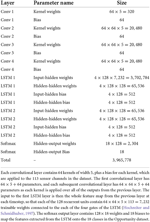
Table 2. This table shows the number of parameters which need to be trained in order to apply DeepConvLSTM to the Opportunity dataset.

For the vast majority of the networks reported in Table 1, any disclosed search strategy used to determine the topology of the DNN was limited to a grid search over a few different numbers of layers or units per layer. Hammerla et al. (2016b) is a counter-example, but their systematic exploration is still limited to ≈ 1,500 configurations while we sample 20,000 per search from a space of 10¹⁶ unique topologies.

Each of these network architectures perform well on their respective datasets, but it is not clear whether they represent the best possible architectures, and which architectural parameters have the largest impact on this performance. An effective NAS method for wearable HAR should therefore be able to explore a search space which at least encompasses the majority of these networks, as well as novel architectures.

2.2. Neural architecture search

So far, most successful NAS algorithms can be divided into three categories—RL (Zhong et al., 2017; Zoph and Le, 2017; Liu et al., 2018a; Pham et al., 2018; Xia and Ding, 2020), evolutionary algorithms (Miikkulainen et al., 2017; Elsken et al., 2019a), and differentiable approaches characterized by a continuous relaxation of structural parameters, which are then optimized by gradient descent (Baker et al., 2017; Zhong et al., 2017; Elsken et al., 2019b). The first two strategies operate on a discrete search space of architectures, and as a consequence both have a very high level of computational complexity (Ren et al., 2020). The latter approach avoids the complexity of a discrete search space, but at the cost of constraining the search space due to the fixed number of nodes. The differentiable approach proposed in DARTS (Liu et al., 2018b) of computing every possible operation during the forward pass of the network in the search phase also leads to very high memory requirements, further constraining the search space on most hardware.

Bayesian Optimization (BO) has also been applied to searching network architectures (Kandasamy et al., 2018; Elsken et al., 2019b), generally using either a Gaussian Process (Ru et al., 2020) or Graph Neural Network (White et al., 2021) to predict the performance of the searched models. BO based algorithms generally are very computationally expensive, but place a greater focus on selecting the best architecture to evaluate at each step (for example, to give the greatest expected improvement) in order to reduce the total number of sampled architectures.

Under the RL paradigm for NAS, introduced in Zoph and Le (2017), a controller network (typically an RNN) is trained to generate suitable classifier architectures, which are then trained and evaluated on a target dataset to give feedback used to train the controller to generate better classifiers (see section 3.1). This method was used to generate competitive convolutional models for image recognition on CIFAR-10. To reduce the computational burden of training many network architectures in a discrete search space, strategies have been proposed to predict converged performance from early validation epochs (Baker et al., 2017; Zhong et al., 2017; Elsken et al., 2019b). The approach used in this paper is closely related to BlockQNN (Zhong et al., 2017).

Recently, NAS methods have also been applied to image-based and skeleton-based activity recognition (Popescu et al., 2020; Zhang et al., 2020), as well as domain-agnostic time-series classification (Rakhshani et al., 2020), with promising results. This work represents the first exploration of NAS with performance prediction for wearable sensor-based HAR.

3. Methodology and experimental setup

3.1. Deep Q learning for NAS

Under the RL paradigm for NAS, a feature extractor is incrementally built by a series of actions chosen at each time step by a controller network. Each action corresponds to adding a layer chosen from 241 options, including convolutional layers (with kernel size in {1,2,3,5,8} and number of kernels in {32,64,128,256}), max pooling layers (with pooling size in {2,3,5}), concatenation of any two previous layers (channel-wise, where mismatched sequence lengths are padded with zeros), and the terminal layer. The terminal layer is an action which can be selected by the controller to indicate that no further layers should be added to the feature extractor. The complete set of actions is indicated in Table 3.

TABLE 3

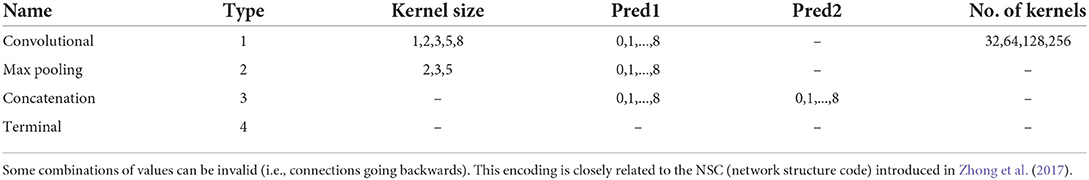
Table 3. Each layer type, parameter, and interconnection is represented by a vector of six elements including the layer ID corresponding to the timestep, and the five elements indicated in the table.

This sequential decision making process is an example of a Markov decision problem (MDP), where the state space is the set of possible network architectures N, the action space is the set of layers L which can be generated at each timestep, and the reward R is a measure of the performance of the classifier network on the target dataset. We refer to the generation and evaluation of one full network architecture as an episode. The reward R can only be obtained after the network has been fully generated, i.e., after the last timestep in each episode. In order to assign rewards to the preceding timesteps, we assume that each layer contributes equally to the final reward (this may not be true—future work may consider assessing how much each layer contributes and weighting the rewards based on this metric).

The goal of this MDP is to find, at each step of the controller network, the layer which maximizes the performance of the complete network—given that all the following layers are selected according to the same policy. We can assign a value to each state-action pair which represents this expected future reward, which we call the Q-value, defined as:

$\begin{array}{ll}q(n,l)=\mathbb{E}[{\displaystyle \sum _{i=t+1}^T}{R}_i|N_t=n,L_t=l],& (1)\end{array}$

where q(n, l) is the Q-value of the layer l appended to network n, t, and T are the current and maximum timestep, and N_t, L_t, R_t the state, action and reward at timestep t. This equation is recursive:

$\begin{array}{lll}q(n,l)& =\mathbb{E}[R_{t+1}+{\displaystyle \sum _{i=t+2}^T}{R}_i|N_t=n,L_t=l]& (2)\end{array}$

$\begin{array}{lll}q(n,l)& =\mathbb{E}[R_{t+1}+q(N_{t+1},L_{t+1})|N_t=n,L_t=l],& (3)\end{array}$

and we can use this property to derive an update rule which allows us to update the Q-value of each chosen action after every episode:

$\begin{array}{ll}Q(N_t,L_t)=Q(N_t,L_t)+\alpha \{R_{t+1}+{\displaystyle \underset{l}{max}}[Q(N_{t+1},l)]-Q(N_t,L_t)\},& (4)\end{array}$

where α is a scaling factor or learning rate which controls the step size of the updates. With deep Q-learning (Mnih et al., 2015), we use a controller DNN to approximate this Q-function by optimizing a loss function which approximates the Q-learning update rule, described in Equation (5). We refer to the term $R_{t+1}+\underset{l}{max}\left[Q(N_{t+1},l)\right]$¹ as the target value.

3.1.1. Search spaces

We define two search spaces, one general search space where a pooling or convolutional layer may be connected to any previously generated layer, allowing for arbitrary skip connections and branches (1.06 × 10¹⁶ architectures), and a restricted feedforward space which only allows for feedforward networks (8.17 × 10¹⁰ architectures), with no concatenations. Many networks of Table 1 can be represented within these search spaces - for example, see Table 4 for the vector encoding of DeepConvLSTM.

TABLE 4

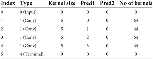
Table 4. Vector encoding of DeepConvLSTM (Ordóñez and Roggen, 2016).

The authors of Hammerla et al. (2016b) use the fANOVA hyperparameter optimization technique to explore a search space of feedforward CNNs with 1–3 layers, where each layer has 16–128 convolutional filters, and the width of the kernels is between 3 and 9 samples. They also use a max pooling layer with kernels of width 2 in all of the networks, and the output of the convolutional layers is processed by a single fully connected layer with 64–2,048 units. These structural hyperparameters are optimized alongside several learning and regularization hyperparameters including the learning rate and the dropout fraction. In total, they sample only 256 network architectures from this search space.

3.1.2. Controller network architecture

The controller network is made up of two RNN layers with 64 units and a linear output layer with 241 units to learn the correlations between layer choices at each timestep and the complete classifier performance (in terms of weighted F1 score), with deep Q learning (Mnih et al., 2015). The value of each output unit is trained to approximate the expected classifier performance when its associated layer is chosen, using the loss function described in section 3.1.3. As such, the number of output units is determined by the number of layers which can be generated in the search space. The input to the controller network is the index of the layer which should be generated, so that the layer chosen is a result of the combination of this knowledge of the position of the layer in the network and the internal dynamics of the RNN, which are informed by the preceding layer choices in the current and previous episodes. Although we have not performed extensive experiments to determine the structure of the DQN, it is probable that this structure has inherent biases which may influence the results. Future work should seek to optimize the controller network architecture.

3.1.3. Training the DQN with experience replay

We train the DQN by sampling batches of 64 past experiences. An experience corresponds to an individual layer generated in a past episode². We train the DQN according to the mean over the batch of the smooth L1 loss (Fu et al., 2019), using the Adam optimizer (Kingma and Ba, 2014). We learn the Q-function using two copies of the Deep Q Network (DQN)—a target DQN with parameters θ^T and a local DQN with parameters θ^L, in order to reduce correlations between the action values and the target values which can cause instability in learning (Mnih et al., 2015). The loss function is given by:

$\begin{array}{ll}Loss=\{\begin{array}{ll}0.5{(x-y)}^2,\hfill & \text{if }|x-y|<1\hfill \\ |x-y|-0.5,\hfill & \text{otherwise}\hfill \end{array}& (5)\end{array}$

where x is the action value predicted by the local net given by $x=\underset{l_t}{max}\left[Q(N_t,l_t,{\theta }^L)\right]$, and y is the target value given by $y=\alpha (R_{t+1}+\underset{l_{t+1}}{max}\left[Q(N_{t+1},l_{t+1},{\theta }^T)\right])$—the combination of the immediate reward and the prediction of the target net at the next timestep, thereby approximating the Q-learning update rule given in Equation (4). The loss is minimized using the Adam optimizer (Kingma and Ba, 2014), a method for stochastic gradient descent which uses the moving average of the gradient and squared gradient of the loss function to compute individual adaptive learning rates for each set of parameters, thereby regulating the step size of the updates. After updating the weights of the local net by backpropagation, we do a “soft update” of the weights of the target net controlled by a parameter τ such that θ^T = (1−τ)θ^T + τθ^L, where we set τ to 10⁻³. This is done every four episodes to improve the stability of training.

ALGORITHM 1

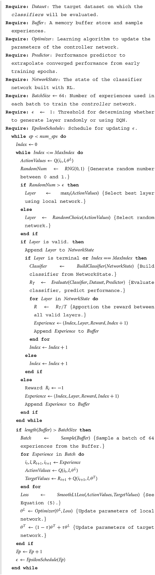
Algorithm 1. Deep neural architecture search with early prediction of converged performance.

3.1.4. Search policy

In order to avoid choosing actions based on low-confidence initial estimates of the Q-values we use an ϵ-greedy policy which chooses the layer with the largest Q-value at each timestep with probability 1−ϵ and a random layer with probability ϵ, which we decay linearly during the training of the controller network from ϵ = 1 to ϵ = 0.01 after 20,000 episodes. This allows us to balance exploration with exploitation of learned knowledge and avoid introducing selection bias into our estimates of the Q-values.

3.1.5. Building the feature extractor

At each RNN timestep t, we sample layers from the search space by feeding the DQN the layer index i_t and choosing a layer according to the ϵ-greedy policy as shown in Figure 1. If the layer chosen is valid³, we increment i and choose another layer, repeating until i = 8, or until the DQN chooses a layer called the terminal layer which indicates that the controller network has decided to stop adding additional layers to the convolutional feature extractor—it has decided that making the classifier network any deeper is likely to degrade the performance.

FIGURE 1

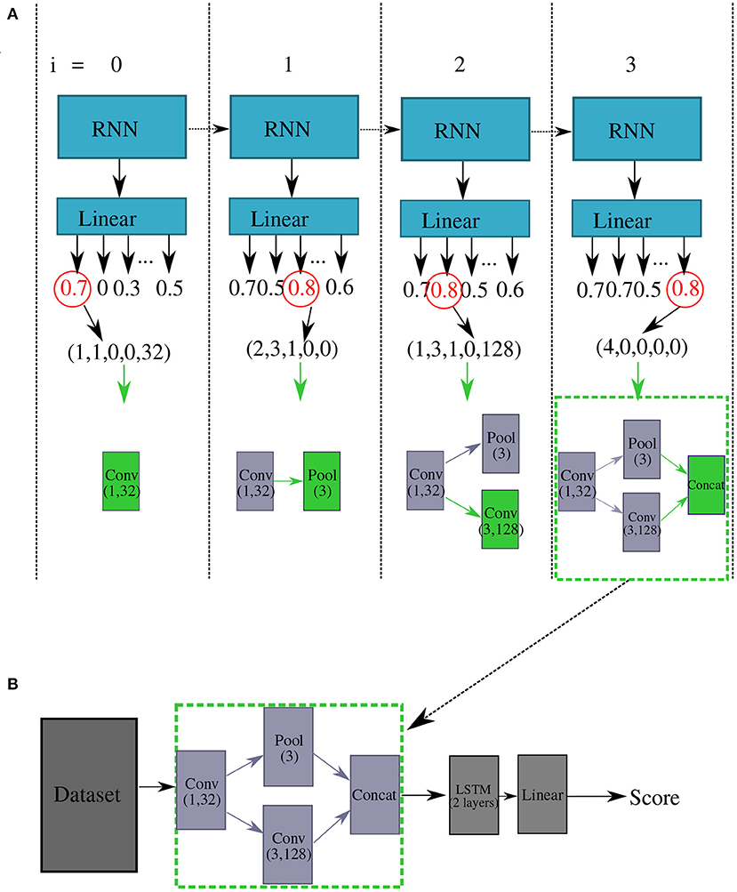
Figure 1. Block diagram which describes how we construct the classifier networks using the DQN. Part (A) shows the actions taken by the DQN to insert layers into the feature extractor. Here, actions are selected with a greedy policy (i.e., ϵ = 0), where the actions with the largest Q-values are selected at each index (circled in red). The network selects the action (Conv, 1, 32, 0), i.e., a convolutional layer with 32 kernels of size 1 connected to the input layer at i = 0. At i = 1, the DQN generates a pooling layer with a width of three samples connected to the first conv layer, denoted as (Pool, 3, 1). At i = 3, the DQN inserts another convolutional layer with 128 kernels of size 3 connected to index 1, and then finally the DQN generates a “terminal” layer at i = 4. This indicates the completion of the feature extractor, which is included in the classifier network as shown in part (B). Once constructed, the network is trained and tested on the target dataset, to produce a reward which is then used to train the DQN.

3.2. Dataset

We train and validate the classifiers on the Opportunity dataset (Roggen et al., 2010), which consists of 6 annotated runs from 4 subjects performing 17 sporadic gestures such as drinking water and opening doors, plus a null class for 18 total activity classes. The activity classes and distribution are explained in Table 5. We use all 113 sensor channels. We split the dataset into a training set and a validation set, consisting of one run from user 1, and we hold out two runs from users 2 and 3 for testing (as in the Opportunity challenge Chavarriaga et al., 2013). In total the training dataset consists of approximately 525,000 samples, while the validation set contains around 32,000 samples and the testing set contains around 119,000 samples.

TABLE 5

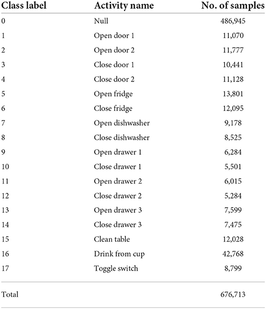
Table 5. Names and distribution of activities in the Opportunity dataset (Roggen et al., 2010).

3.3. Evaluation of classifiers

To evaluate the feature extractor, we combine it with a two layer LSTM recurrent network with 128 units per layer and a single linear classification layer with softmax output. This is almost identical to the output structure of DeepConvLSTM (we do not use dropout). We use a sliding window size of 500 ms (16 samples, twice the maximum kernel length), where the state of the LSTM is reset after each window. The network output is compared to the ground truth at the last sample of each window. The learning rate of each classifier network is set at 1 × 10⁻³, and we use a batch size of 100, the same as DeepConvLSTM.

We take the F1 score achieved on the validation set as the reward R_T for each episode, where T is the number of layers in the feature extractor. We allocate this reward evenly over each valid layer, setting the reward for each valid layer i to be $R_i=\frac{R_T}{T}$. If the controller network tries to generate a layer with a connection to a network which does not exist, this layer receives a reward of −1. Note that the total reward R_i can only be positive as it is constructed by considering only valid layers.

3.3.1. Testing on unseen data

Testing is performed on selected networks after the search to prevent overfitting to the test set—we show only the validation set to classifiers during the search process to get an estimate of their performance. The best generated models are then trained to convergence for 300 epochs, or until their validation F1 score has not improved over 30 epochs (this resulted in an average of around 100–150 epochs to train to convergence). The performance of the best models on the testing set is shown in Table 6.

TABLE 6

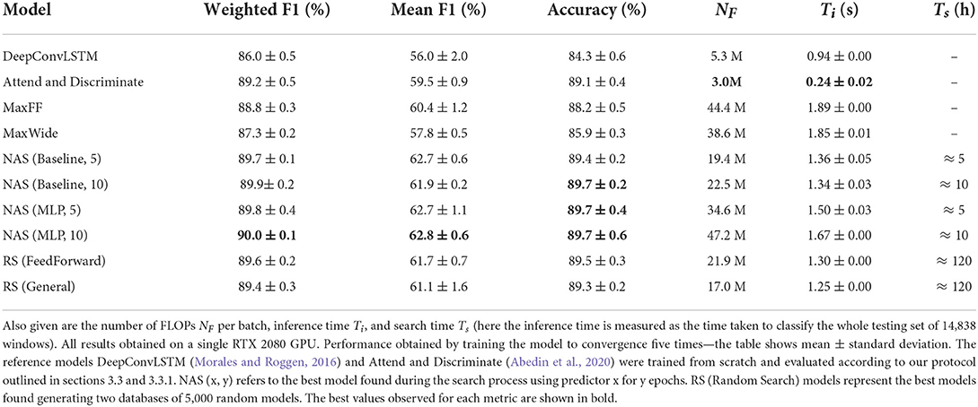
Table 6. Weighted F1 score, mean F1 score, and accuracy score achieved by various architectures.

3.4. Converged performance estimation

In order to minimize computation time, we employ neural regression networks to approximate the true reward after training the classifier models for only a few epochs. As well as the training and validation statistics, we incorporate information about the structure of the classifiers and their computational complexity [approximated by the number of floating point operations (FLOPs) per inference]. We propose four prediction methods, illustrated in Figure 2:

• MLP: A three layer perceptron with 64 units per layer, which takes as input the training loss and the validation loss, accuracy, class weighted F1 score, and mean F1 score at every training epoch, as well as the density (number of connections between layers divided by number of layers) and number of FLOPs of the subject. See Figure 2A.

• CNN: A branched convolutional network with a core structure the same as above, and an additional convolutional input layer with 64 kernels of size three which takes the training and validation statistics as a time-series input, and incorporates the density and number of FLOPs at the second layer. See Figure 2B.

• MLP (struct): A variant of the MLP which additionally takes the vector representation of the network structure as an input. See Figure 2C.

• CNN (struct): A variant of the CNN which takes a vector representation of the network structure as an additional input. See Figure 2D.

FIGURE 2

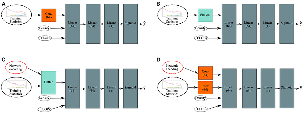
Figure 2. The structures of the tested regression networks, with input data depicted. (A) Multi-layer perceptron (MLP) model. (B) Convolutional neural network (CNN) model. (C) MLP model with additional structural information. (D) CNN model with additional structural information.

We compare these methods against a baseline method which simply uses the mean validation F1 score over the five last training epochs (i.e., epochs 5–10 if training for 10 epochs) as the reward.

We generated, trained to convergence and tested 5,000 randomly sampled networks from each of the general and feedforward search spaces, collecting training and validation statistics to produce two databases of models. The generation of these two databases took approximately 120 h each. The distribution of scores within each model database are shown in Figure 3. We trained the predictors to minimize the MSE loss between predicted and actual testing F1 score, and we weighted the loss function according to the testing F1 score since we are chiefly interested in the best performing models. To assess the performance of the predictors, we performed a 10-fold cross-validation experiment on each database of models.

FIGURE 3

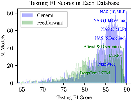
Figure 3. Density plot of testing F1 scores from 5,000 randomly generated networks within the general and feedforward search space, annotated with F1 scores from benchmark models. The y-axis represents the number of models in each bin (where each bin is 0.01% F1 score). Blue or green text indicates that these models are contained within the general or feedforward search space, respectively. “NAS (x,y)” refers to the best model found by NAS, when using x epochs and y method to predict scores. Other vertical lines represent models which we have implemented, trained, and tested using the protocol described in sections 3.3 and 3.3. as references, including DeepConvLSTM (Ordóñez and Roggen, 2016) and Attend and Discriminate (Abedin et al., 2020).

4. Results

4.1. Performance prediction

To analyze the results, we split the database of models from the general search space into five bins based on their testing F1 scores. The rank correlations achieved by each predictive model on each partition of data are shown in the top part of Figure 4. All of our prediction methods achieve better overall correlations than the baseline, and in addition they all achieve significantly better correlations in the high performance group (top 20% of networks), indicating that they are able to identify and distinguish between high performing networks in early training epochs much better than the baseline. The best performing predictor at five epochs is the MLP, with a correlation of 0.54 on the top 20% of models compared to a baseline correlation of 0.17.

FIGURE 4

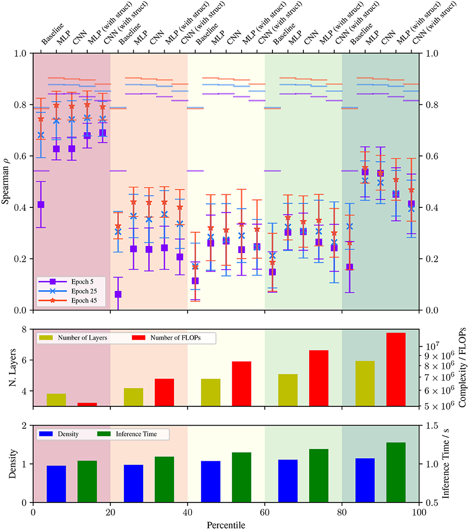
Figure 4. Fold-averaged (10-fold) spearman rank correlation coefficient with the converged F1 score achieved by various performance prediction methods on the general database when using data up to epoch 5, 25, and 45, split into groups by testing performance (from worst 20% of models on the left to best 20% on the right). The error bars represent the standard deviation over the folds, and the overall correlation at each epoch is indicated by a horizontal line. The bottom two subplots show the average depth, complexity, graph density, and inference time for each group of models within the general database.

From the bottom sections of Figure 4, we can see that there is a significant positive correlation between the testing performance of the classifiers we looked at and their computational complexity (the top 20% have over double the average FLOPs of the bottom 20%) and number of layers (from ≈4 to ≈6). We also observe a more modest increase in the node density and inference time of high performing classifiers, indicating deep networks with a few branches perform the best.

4.2. Neural architecture search

We performed four explorations of the search space, using the MLP and baseline prediction methods, and training the classifier models for 5 and 10 epochs. Table 6 shows the weighted F1 score, mean F1 score and accuracy of the best models found in each search run, as well as the inference time, number of FLOPs, and time taken to search. Alongside these, we also present the same metrics for four benchmark models DeepConvLSTM, Attend and Discriminate, MaxFF, and MaxWide, trained and tested under the same conditions as the NAS-generated architectures.

DeepConvLSTM refers to an implementation of the feature extractor part of DeepConvLSTM (Ordóñez and Roggen, 2016). Attend and Discriminate is a state of the art model iterating on the architecture of DeepConvLSTM, which uses an attentional gated recurrent unit (GRU) instead of LSTM recurrent section, uses center-loss to maximize the distance between class centers in the feature space (Wen et al., 2016), and also implements a novel self-attention layer, a channel interaction encoder (CIE) to take advantage of correlations between channels in the output of the feature extractor (Abedin et al., 2020). The structure of the convolutional feature extractor is otherwise the same as DeepConvLSTM. MaxFF refers to a feedforward model with eight convolutional layers, each with 256 kernels of size 5, while MaxWide refers to a model with eight parallel convolutional layers with 256 kernels of size 5, thereby representing the deepest and widest limits of the search space.

From Table 6, the NAS-generated models outperform the benchmark models on this task in all cases. The best feature extractor, shown in Figure 5 and in vector form in Table 7, was found using NAS with the MLP predictor, using 10 epochs of validation data. The best feature extractor has a large variety of convolutional kernel sizes, does not include any pooling layers, and uses a branched structure. The NAS generated models also have lower complexity than the two “Max” benchmark models, but significantly higher complexity than DeepConvLSTM and Attend and Discriminate. Attend and Discriminate performs much better than DeepConvLSTM and has a far lower inference time than any of the other models, as well as significantly lower FLOPs. This may be attributed to the GRU recurrent section, which has 1/4 of the parameters of the LSTM, and the CIE self-attention layer which effectively compresses the output of the convolutional feature extractor.

FIGURE 5

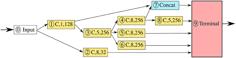
Figure 5. The network architecture of the best feature extractor generated by NAS with MLP performance predictor. C, x, y denotes a convolutional layer with y kernels of size x.

TABLE 7

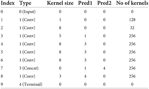
Table 7. Vector encoding of the best model found by our NAS algorithm using the MLP predictor and training each subject model for 10 epochs, after 20k sampled models.

We have used the class-weighted F1 score to draw our major conclusions in this study, for consistency and ease of comparison with previous publications (Ordóñez and Roggen, 2016). In the Opportunity dataset, where around 70% of the samples are of the null class, this metric will be biased toward the null class. To support our results, we also report the mean F1 score and accuracy of each model in Table 6. The mean F1 score tends to be lower than the weighted F1 score, with a range of around 56–63%, compared to 86–90% for the latter. This suggests that the null class is easier to classify than the other classes in the dataset. In terms of mean F1 score, the same model performs the best overall (the NAS with MLP predictor and 10 training epochs), while the baseline NAS with only five training epochs performs better than the 10 epoch version, within 0.1% F1 score of the best model. While the mean F1 score may better represent the performance of the network on the more difficult activity classes, it also generally has a much larger standard deviation, making comparisons between different models more difficult.

5. Discussion

While we have only applied our methods to one dataset, in principle the NAS and performance prediction methods are completely transferable to other datasets—it would simply be necessary to swap out the dataset in Figure 6, and adapt the kernel and pooling sizes in the search space to suit the new dataset. The performance prediction algorithm we have proposed would also need to be re-trained on the new dataset. In order to validate the results obtained in this study, future work should include applying the algorithm to a variety of additional datasets. We chose to evaluate our method on the Opportunity dataset because it contains sporadic, short duration activities which are very hard to correctly classify, and therefore represents a challenging application for a NAS algorithm. Other datasets may be more suited for determining the generalization ability of the networks, since the Opportunity dataset contains only four subjects.

FIGURE 6

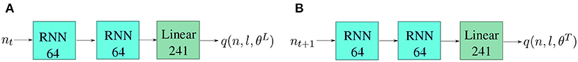
Figure 6. The network architectures of the two identical DQNs used as local and target networks. Both consist of two recurrent layers with 64 units followed by a linear output layer mapping the output of the recurrent cells onto the number of possible layers in the action space to produce Q-values for each possible action. The local network predicts the q-values at the current timestep t and these values are used to select a layer to generate. The target network predicts the q-values at the next timestep t + 1, given the layer selected by the local network. These values are summed with the immediate reward R_{t + 1} to give the target values which the DQN is trained toward (illustrated in Equation 4). θ^L and θ^T represent the parameters of the local and target networks, respectively.

Although we find that our NAS method can generate better architectures than a random search in considerably less time, and that both produce networks which perform better than our implementations of DeepConvLSTM (Ordóñez and Roggen, 2016) and Attend and Discriminate (Abedin et al., 2020), these implementations performed significantly worse than reported in the literature (Hammerla et al., 2016a; Ordóñez and Roggen, 2016; Guan and Plötz, 2017; Abedin et al., 2020), and thus we were not able to show an improvement over the state-of-the-art F1 score—this is likely due to differences in the training and testing protocols used. Further, we only apply our Q learning method to the optimization of the structural hyperparameters of the network, leaving out several parameters which may also have a large impact on the performance of the network, including the batch size and learning rate. For these hyperparameters, we chose to use the same values (given in section 3.3) as DeepConvLSTM used on the Opportunity dataset, for a fair comparison against the state of the art. This highlights a problem also discussed in Elsken et al. (2019b), namely that there are more factors than the architecture of a network which affect it's performance. This indicates a need for a common benchmark for NAS on HAR datasets, following the examples of Dong and Yang (2020) for computer vision and Klyuchnikov et al. (2020) for natural language processing, which would allow us to test NAS methods on a search space of pre-trained and pre-evaluated models.

Although our performance estimators achieve much better rank correlations than the baseline when predicting converged performance (see Figure 4), this translated to only a marginally better searched feature extractor. This indicates that more work is needed to find better predictors which further improve the NAS results. While the performance estimators enabled the NAS algorithm to be run much more quickly, generation of the random databases of models themselves took ≈ 120 h, comparable to the total time taken by the random search. Fortunately, once trained, the performance estimators can be re-used multiple times, saving a lot of compute in the long run.

The performance estimators were trained to map the performance of a given classifier model on the validation set to its performance on the test set. In the real world, the distribution of test data is often very different from the distribution of available training data. This is a problem encountered by all machine learning methods for HAR. The best way to solve this problem is to increase the diversity of the training data—however, the performance predictors could also be extended to predict the generalization of a model to other subjects.

The state of the art model Attend and Discriminate achieved performance close to that of the NAS generated models with significantly lower complexity in terms of the number of FLOPs, and much faster inference. This indicates that future NAS studies could benefit from including GRU recurrent units and CIE self-attention mechanisms in the search space.

Another approach to reducing the complexity of the search would be to modify the algorithm to operate on a continuous search space of network architectures, for example using unsupervised representation learning to encode the search space into a continuous latent space, which can then be sampled from by the NAS algorithm (Yan et al., 2020).

In this study, we have chosen to search for the convolutional feature extractor part of a DeepConvLSTM-like network, in order to keep the size of the search space manageable for an initial characterization. The method could in theory be applied to other search spaces including searching for recurrent cell structures. This study represents the first time any NAS algorithm has been applied to HAR from wearable sensors. Future work should consider evaluating other NAS algorithms including Bayesian Optimization and Genetic Algorithms.

5.1. Implementation details

All of the experiments reported in this paper were performed using a single Nvidia RTX-2080 GPU. All of the code for the generation of DNNs was implemented using PyTorch and the RL logic was implemented in a custom OpenAI gym environment. To avoid performing the computationally expensive evaluation of the same classifier network many times over, we stored the results from each evaluated network. Once the same network had been evaluated three times, we took the average of the three scores and used this as the reward if the same network were to be generated again.

Although an exhaustive search of the space of possible networks appears out of reach using desktop equipment (our random search of 5,000 models took over 100 h, see Table 6), our work shows that using performance estimators to predict the converged performance in early training epochs can significantly reduce the technical requirements, reducing the search time to less than 10 h while maintaining the quality of the results.

6. Conclusions

We have proposed a NAS method for designing convolutional feature extractors for deep recurrent neural networks using Deep Q Learning, and shown that our NAS-guided search was able to find feature extractor algorithms which beat our implementation of DeepConvLSTM by up to 4% F1 score and the state-of-the-art model Attend and Discriminate by 0.8% on the Opportunity dataset, and which beat the naive maximum complexity algorithms we propose by 1–3% F1 score. We also achieved 0.4% better F1 score than the best model found in a random search, while reducing the search time by more than 90% through the use of a neural regression based performance estimator.

This work represents a significant step in demonstrating the viability of NAS methods for designing more powerful DNN architectures for wearable HAR applications. While the use of a RL agent to construct DNN architectures has been proposed previously for image recognition applications (Zoph and Le, 2017), it has not previously been applied to HAR from wearable sensors. Many modifications were made to the algorithm to adapt it to the wearable HAR domain. As well as implementing a custom search space containing convolutional and pooling layers chosen with reference to state of the art models, we also combine the NAS-generated convolutional networks with a fixed-architecture LSTM network inspired by previous works (Inoue et al., 2016; Morales and Roggen, 2016; Guan and Plötz, 2017; Abedin et al., 2020) to further tailor the generated networks to the wearable HAR domain.

We found that our NAS-generated models were consistently larger and more complex than state-of-the-art models, indicating a need for future research focusing on reducing the complexity of solutions.

6.1. Future work

One promising approach to reducing the complexity of the searched architectures would be multi-objective reinforcement learning (MORL), either using a scalarization function (Miettinen and Mäkelä, 2002) to combine multiple rewards into a single scalar reward, or using a multi-policy algorithm to search for a set of optimal solutions in each run (Barrett and Narayanan, 2008). An example would be to take the F1 score of the models as one reward function R_F1 and the number of FLOPs R_FLOPs as another, then combine the two with a scalarization function (for example constructing a combined reward R = R_F1−R_FLOPs). This technique could be applied with other metrics such as the inference time or the size of the model in memory in order to find network architectures which can perform real-time inference on embedded systems while maintaining high performance.

The complexity of the search and of the final models could further be reduced by considering architectures for each sensor or each sensor modality in a dataset. This could be achieved by including the sensor position or sensor modality in the state which is given to the DQN each timestep, making the choice of layer dependent on the sensor modality and position. This could be an effective approach for applications where there are multiple sensor modalities with different sample rates, since these would likely have different optimal architectures. These sensor-specific architectures could be combined into ensemble classifiers or into larger DNNs containing multiple branches. It would also be interesting to investigate whether the sensor modality specific architectures would be more effective at generalizing to other datasets using the same modalities. Going further, it has been shown that the individual axes of a tri-axial accelerometer can each contribute more or less to the recognition of specific activities (Javed et al., 2020), which could be exploited by searching for channel-specific network architectures.

Validation of this and similar methods on a larger variety of target HAR datasets should also be a priority, and future work could also include development of cross-dataset performance estimators taking into account factors such as sample rate and activity duration/periodicity to identify network blocks and architectures which are broadly applicable over many similar applications. For example, it can be assumed that a CNN will perform best when the length of the convolutional kernels is equal to or larger than the length of the activities in the target dataset. A general performance estimator should therefore be able to learn and apply this and subtler correlations to quickly predict the converged performance of a DNN. Research in this direction is very important to reduce the technical barrier of entry for future NAS methods.

Going forward, the search space should also be expanded both to optimize the recurrent section of the network and to consider recent advances such as self-attention mechanisms (Abedin et al., 2020). Additionally, unsupervised representation learning of network architectures should be considered as a viable way to improve the accuracy of performance prediction methods and potentially to encode a large discrete search space of network architectures into a continuous latent space (Yan et al., 2020).

Data availability statement

The raw data supporting the conclusions of this article will be made available by the authors, without undue reservation.

Author contributions

LP designed and carried out the experiments reported in the article and wrote the manuscript. DR provided supervision and guidance during the experimental phase of the research and extensive editing of the manuscript.

Acknowledgments

This work was partially funded by the EU H2020-ICT-2019-3 project HumanE AI Net (project number 952026). The content of this manuscript has been presented in part at the International Symposium on Wearable Computing 2021 (Pellatt and Roggen, 2021).

Conflict of interest

The authors declare that the research was conducted in the absence of any commercial or financial relationships that could be construed as a potential conflict of interest.

Publisher's note

All claims expressed in this article are solely those of the authors and do not necessarily represent those of their affiliated organizations, or those of the publisher, the editors and the reviewers. Any product that may be evaluated in this article, or claim that may be made by its manufacturer, is not guaranteed or endorsed by the publisher.

Footnotes

1. ^N_t here represents the network state, including both the internal dynamics of the RNN which encodes information about the previous layers chosen, as well as the explicit input to the RNN which is the index of the current layer.

2. ^Technically, the experiences consist of the state (layer index), action (selected layer), reward (F1 score of the completed classifier), and next state (the next index), as shown in Algorithm 1. This is everything needed to compute the loss and perform one training step of the controller network.

3. ^A “valid” layer is a layer which can be connected to its inputs. An invalid layer would be, for example, the first layer wanting to be connected to the second layer (recurrent connection).

References

Abedin, A., Ehsanpour, M., Shi, Q., Rezatofighi, H., and Ranasinghe, D. C. (2020). Attend and discriminate: beyond the state-of-the-art for human activity recognition using wearable sensors. arXiv:2007.07172.. doi: 10.48550/arXiv.2007.07172

CrossRef Full Text | Google Scholar

Anguita, D., Ghio, A., Oneto, L., Parra, X., and Reyes-Ortiz, J. L. (2013). “A public domain dataset for human activity recognition using smartphones,” in 21st European Symposium on Artificial Neural Networks, Computational Intelligence And Machine Learning, Vol. 3 (Bruges).

Google Scholar

Bachlin, M., Plotnik, M., Roggen, D., Maidan, I., Hausdorff, J. M., Giladi, N., et al. (2010). Wearable assistant for Parkinson's disease patients with the freezing of gait symptom. IEEE Trans. Inform. Technol. Biomed. 14, 436–446. doi: 10.1109/TITB.2009.2036165

PubMed Abstract | CrossRef Full Text | Google Scholar

Baker, B., Gupta, O., Raskar, R., and Naik, N. (2017). Accelerating neural architecture search using performance prediction. arXiv:1705.10823v2. doi: 10.48550/arXiv.1705.10823

CrossRef Full Text | Google Scholar

Banos, O., Garcia, R., Holgado-Terriza, J. A., Damas, M., Pomares, H., Rojas, I., et al. (2014a). “mhealthdroid: A novel framework for agile development of mobile health applications,” in International Workshop on Ambient Assisted Living, eds L. Pecchia, L. L. Chen, C. Nugent, J. Bravo (Cham: Springer), 91–98. doi: 10.1007/978-3-319-13105-4_14

PubMed Abstract | CrossRef Full Text | Google Scholar

Banos, O., Toth, M. A., Damas, M., Pomares, H., and Rojas, I. (2014b). Dealing with the effects of sensor displacement in wearable activity recognition. Sensors 14, 9995–10023. doi: 10.3390/s140609995

PubMed Abstract | CrossRef Full Text | Google Scholar

Barrett, L., and Narayanan, S. (2008). “Learning all optimal policies with multiple criteria,” in Proceedings of the 25th International Conference on Machine Learning, ICML '08 (New York, NY: Association for Computing Machinery), 41–47. doi: 10.1145/1390156.1390162

CrossRef Full Text | Google Scholar

Bulling, A., Blanke, U., and Schiele, B. (2014). A tutorial on human activity recognition using body-worn inertial sensors. ACM Comput. Surv. 46, 1–33. doi: 10.1145/2499621

CrossRef Full Text | Google Scholar

Chavarriaga, R., Sagha, H., Calatroni, A., Digumarti, S. T., Tröster, G., Millán, J. d. R., et al. (2013). The opportunity challenge: a benchmark database for on-body sensor-based activity recognition. Pattern Recognit. Lett. 34, 2033–2042. doi: 10.1016/j.patrec.2012.12.014

CrossRef Full Text | Google Scholar

Chen, K., Yao, L., Zhang, D., Wang, X., Chang, X., and Nie, F. (2020a). A semisupervised recurrent convolutional attention model for human activity recognition. IEEE Trans. Neural Netw. Learn. Syst. 31, 1747–1756. doi: 10.1109/TNNLS.2019.2927224

PubMed Abstract | CrossRef Full Text | Google Scholar

Chen, L., Zhang, Y., and Peng, L. (2020b). METIER: a deep multi-task learning based activity and user recognition model using wearable sensors. Proc. ACM Interact. Mob. Wearable Ubiquitous Technol. 4, 1–18. doi: 10.1145/3381012

CrossRef Full Text | Google Scholar

Cho, H., and Yoon, S. M. (2018). Divide and conquer-based 1D CNN human activity recognition using test data sharpening. Sensors 18:1055. doi: 10.3390/s18041055

PubMed Abstract | CrossRef Full Text | Google Scholar

Cook, D. J., Crandall, A. S., Thomas, B. L., and Krishnan, N. C. (2013). Casas: a smart home in a box. Computer 46, 62–69. doi: 10.1109/MC.2012.328

PubMed Abstract | CrossRef Full Text | Google Scholar

Dong, X., and Yang, Y. (2020). Nas-bench-201: extending the scope of reproducible neural architecture search. arXiv preprint arXiv:2001.00326. doi: 10.48550/arXiv.2001.00326

CrossRef Full Text | Google Scholar

Elsken, T., Metzen, J. H., and Hutter, F. (2019a). Efficient multi-objective neural architecture search via lamarckian evolution. arXiv:1804.09081. doi: 10.48550/arXiv.1804.09081

CrossRef Full Text | Google Scholar

Elsken, T., Metzen, J. H., Hutter, F., et al. (2019b). Neural architecture search: a survey. J. Mach. Learn. Res. 20, 1–21. doi: 10.1007/978-3-030-05318-5_11

CrossRef Full Text | Google Scholar

Fu, C., Shvets, M., and Berg, A. C. (2019). Retinamask: learning to predict masks improves state-of-the-art single-shot detection for free. arXiv preprint. arXiv:1901.03353. doi: 10.48550/arXiv.1901.03353

CrossRef Full Text | Google Scholar

Guan, Y., and Plötz, T. (2017). Ensembles of deep lstm learners for activity recognition using wearables. Proc. ACM Interact. Mob. Wearable Ubiquitous Technol. 1, 1–28. doi: 10.1145/3090076

CrossRef Full Text | Google Scholar

Hammerla, N. Y., Halloran, S., and Ploetz, T. (2016a). Deep, convolutional, and recurrent models for human activity recognition using wearables. arXiv:1604.08880. doi: 10.48550/arXiv.1604.08880

CrossRef Full Text | Google Scholar

Hammerla, N. Y., Halloran, S., and Plötz, T. (2016b). “Deep, convolutional, and recurrent models for human activity recognition using wearables,” in Proceedings of the Twenty-Fifth International Joint Conference on Artificial Intelligence (New York, NY), 1533–1540.

Google Scholar

Hochreiter, S., and Schmidhuber, J. (1997). Long short-term memory. Neural Comput., 9, 1735–1780. doi: 10.1162/neco.1997.9.8.1735

PubMed Abstract | CrossRef Full Text | Google Scholar

Hossain, H. M. S., Al Haiz Khan, M. A., and Roy, N. (2018). Deactive: scaling activity recognition with active deep learning. Proc. ACM Interact. Mob. Wearable Ubiquitous Technol. 2, 1–23. doi: 10.1145/3214269

CrossRef Full Text | Google Scholar

Huynh, T., Fritz, M., and Schiele, B. (2008). “Discovery of activity patterns using topic models,” in Proceedings of the 10th International Conference on Ubiquitous Computing (Seoul), 10–19. doi: 10.1145/1409635.1409638

CrossRef Full Text | Google Scholar

Inoue, M., Inoue, S., and Nishida, T. (2016). Deep recurrent neural network for mobile human activity recognition with high throughput. arXiv:1611.03607. doi: 10.48550/arXiv.1611.03607

CrossRef Full Text | Google Scholar

Javed, A. R., Sarwar, M. U., Khan, S., Iwendi, C., Mittal, M., and Kumar, N. (2020). Analyzing the effectiveness and contribution of each axis of tri-axial accelerometer sensor for accurate activity recognition. Sensors 20:2216. doi: 10.3390/s20082216

PubMed Abstract | CrossRef Full Text | Google Scholar

Jiang, W., and Yin, Z. (2015). “Human activity recognition using wearable sensors by deep convolutional neural networks,” in Proceedings of the 23rd ACM International Conference on Multimedia, MM '15 (New York, NY: ACM), 1307–1310.

PubMed Abstract | Google Scholar

Kandasamy, K., Neiswanger, W., Schneider, J., Poczos, B., and Xing, E. P. (2018). “Neural architecture search with bayesian optimisation and optimal transport,” in 32nd Conference on Neural Information Processing Systems (NeurIPS 2018) (Montreal), 2016–2025.

Google Scholar

Kawaguchi, N., Ogawa, N., Iwasaki, Y., Kaji, K., Terada, T., Murao, K., et al. (2011). “Hasc challenge: gathering large scale human activity corpus for the real-world activity understandings,” in AH '11: Proceedings of the 2nd Augmented Human International Conference (Tokyo), 1–5. doi: 10.1145/1959826.1959853

CrossRef Full Text | Google Scholar

Kingma, D. P., and Ba, J. (2014). Adam: a method for stochastic optimization. arXiv preprint arXiv:1412.6980. doi: 10.48550/arXiv.1412.6980

CrossRef Full Text | Google Scholar

Klyuchnikov, N., Trofimov, I., Artemova, E., Salnikov, M., Fedorov, M., and Burnaev, E. (2020). Nas-bench-nlp: neural architecture search benchmark for natural language processing. IEEE Access. 10, 45736–45747. doi: 10.1109/access.2022.3169897

CrossRef Full Text | Google Scholar

Li, L., Khodak, M., Balcan, M.-F., and Talwalkar, A. (2020). Geometry-aware gradient algorithms for neural architecture search. arXiv:2004.07802v5. doi: 10.48550/arXiv.2004.07802

CrossRef Full Text | Google Scholar

Liu, C., Zoph, B., Neumann, M., Shlens, J., Hua, W., Li, L.-J., et al. (2018a). “Progressive neural architecture search,” in Proceedings of the European Conference on Computer Vision (ECCV), Vol. 11205, eds V. Ferrari, M. Hebert, C. Sminchisescu, and Y. Weiss (Cham: Springer), 19–34. doi: 10.1007/978-3-030-01246-5_2

CrossRef Full Text | Google Scholar

Liu, H., Simonyan, K., and Yang, Y. (2018b). DARTS: differentiable architecture search. arXiv:1806.09055. doi: 10.48550/arXiv.1806.09055

CrossRef Full Text | Google Scholar

Lu, C. X., Du, B., Wen, H., Wang, S., Markham, A., Martinovic, I., et al. (2018). Snoopy: sniffing your smartwatch passwords via deep sequence learning. Proc. ACM Interact. Mob. Wearable Ubiquitous Technol. 1, 1–29. doi: 10.1145/3161196

CrossRef Full Text | Google Scholar

Malekzadeh, M., Clegg, R. G., Cavallaro, A., and Haddadi, H. (2019). “Mobile sensor data anonymization,” in Proceedings of the International Conference on Internet of Things Design and Implementation, IoTDI '19 (New York, NY: ACM), 49–58. doi: 10.1145/3123021.3123046

PubMed Abstract | CrossRef Full Text | Google Scholar

Malekzadeh, M., Clegg, R. G., Cavallaro, A., and Haddadi, H. (2021). Dana: dimension-adaptive neural architecture for multivariate sensor data. arXiv:2008.02397v4. doi: 10.1145/3478074

CrossRef Full Text | Google Scholar

Micucci, D., Mobilio, M., and Napoletano, P. (2016). Unimib SHAR: a new dataset for human activity recognition using acceleration data from smartphones. arXiv:1611.07688. doi: 10.48550/arXiv.1611.07688

CrossRef Full Text | Google Scholar

Miettinen, K., and Mäkelä, M. M. (2002). On scalarizing functions -0-in multiobjective optimization. OR Spectr. 24, 193–213. doi: 10.1007/s00291-001-0092-9

CrossRef Full Text | Google Scholar

Miikkulainen, R., Liang, J., Meyerson, E., Rawal, A., Fink, D., Francon, O., et al. (2017). arXiv:1703.00548v2. doi: 10.48550/arXiv.1703.00548

CrossRef Full Text | Google Scholar

Mnih, V., Kavukcuoglu, K., Silver, D., Rusu, A. A., Veness, J., Bellemare, M. G., et al. (2015). Human-level control through deep reinforcement learning. Nature 518, 529–533. doi: 10.1038/nature14236

PubMed Abstract | CrossRef Full Text | Google Scholar

Morales, F. J. O., and Roggen, D. (2016). “Deep convolutional feature transfer across mobile activity recognition domains, sensor modalities and locations,” in Proceedings of the 2016 ACM International Symposium on Wearable Computers, ISWC '16 (New York, NY: Association for Computing Machinery), 92–99.

Google Scholar

Münzner, S., Schmidt, P., Reiss, A., Hanselmann, M., Stiefelhagen, R., and Dürichen, R. (2017). “CNN-based sensor fusion techniques for multimodal human activity recognition,” in Proceedings of the 2017 ACM International Symposium on Wearable Computers, ISWC '17 (New York, NY: Association for Computing Machinery), 158–165.

PubMed Abstract | Google Scholar

Ordóñez, F. J., and Roggen, D. (2016). Deep convolutional and LSTM recurrent neural networks for multimodal wearable activity recognition. Sensors 16:115. doi: 10.3390/s16010115

PubMed Abstract | CrossRef Full Text | Google Scholar

Pellatt, L., and Roggen, D. (2021). “Fast deep neural architecture search for wearable activity recognition by early prediction of converged performance,” in 2021 International Symposium on Wearable Computers, (New York, NY: Association for Computing Machinery), 1–6. doi: 10.1145/3460421.3478813

CrossRef Full Text | Google Scholar

Peng, L., Chen, L., Ye, Z., and Zhang, Y. (2018). Aroma: a deep multi-task learning based simple and complex human activity recognition method using wearable sensors. Proc. ACM Interact. Mob. Wearable Ubiquitous Technol. 2, 1–16. doi: 10.1145/3214277

CrossRef Full Text | Google Scholar

Pham, H., Guan, M. Y., Zoph, B., Le, Q. V., and Dean, J. (2018). Efficient neural architecture search via pa=rameter sharing. arXiv:1802.03268v2. doi: 10.48550/arXiv.1802.03268

CrossRef Full Text | Google Scholar

Popescu, A.-C., Mocanu, I., and Cramariuc, B. (2020). Fusion mechanisms for human activity recognition using automated machine learning. IEEE Access. 8, 143996–144014. doi: 10.1109/ACCESS.2020.3013406

CrossRef Full Text | Google Scholar

Rakhshani, H., Ismail Fawaz, H., Idoumghar, L., Forestier, G., Lepagnot, J., Weber, J., et al. (2020). “Neural architecture search for time series classification,” in 2020 International Joint Conference on Neural Networks (IJCNN) (Glasgow, UK).

Google Scholar

Reiss, A., and Stricker, D. (2012). “Introducing a new benchmarked dataset for activity monitoring,” in 2012 16th International Symposium on Wearable Computers, IEEE (Newcastle, UK), 108–109.

Google Scholar

Ren, P., Xiao, Y., Chang, X., Huang, P., Li, Z., Chen, X., et al. (2020). A comprehensive survey of neural architecture search: challenges and solutions. arXiv:2006.02903v3. doi: 10.48550/arXiv.2006.02903

CrossRef Full Text | Google Scholar

Reyes-Ortiz, J.-L., Oneto, L., Samà, A., Parra, X., and Anguita, D. (2016). Transition-aware human activity recognition using smartphones. Neurocomputing 171, 754–767. doi: 10.1016/j.neucom.2015.07.085

CrossRef Full Text | Google Scholar

Roggen, D., Calatroni, A., Rossi, M., Holleczek, T., Förster, K., Tröster, G., et al. (2010). “Collecting complex activity datasets in highly rich networked sensor environments,” in 2010 Seventh International Conference on Networked Sensing Systems (INSS) (Kassel), 233–240. doi: 10.1109/INSS.2010.5573462

CrossRef Full Text | Google Scholar

Ronao, C. A., and Cho, S.-B. (2016). Human activity recognition with smartphone sensors using deep learning neural networks. Expert Syst. Appl. 59, 235–244. doi: 10.1016/j.eswa.2016.04.032

CrossRef Full Text | Google Scholar

Ru, B., Wan, X., Dong, X., and Osborne, M. (2020). Neural architecture search using bayesian optimisation with Weisfeiler-Lehman kernel. arXiv:2006.07556v2. doi: 10.48550/arXiv.2006.07556

CrossRef Full Text | Google Scholar

Saeed, A., Ozcelebi, T., and Lukkien, J. (2019). Multi-task self-supervised learning for human activity detection. Proc. ACM Interact. Mob. Wearable Ubiquitous Technol. 3, 1–30. doi: 10.1145/3328932

CrossRef Full Text | Google Scholar

Shoaib, M., Bosch, S., Incel, O. D., Scholten, H., and Havinga, P. J. (2014). Fusion of smartphone motion sensors for physical activity recognition. Sensors 14, 10146–10176. doi: 10.3390/s140610146

PubMed Abstract | CrossRef Full Text | Google Scholar

Stisen, A., Blunck, H., Bhattacharya, S., Prentow, T. S., Kjærgaard, M. B., Dey, A., et al. (2015). “Smart devices are different: assessing and mitigating mobile sensing heterogeneities for activity recognition,” in Proceedings of the 13th ACM Conference on Embedded Networked Sensor Systems (Seoul), 127–140. doi: 10.1145/2809695.2809718

CrossRef Full Text | Google Scholar

Vavoulas, G., Chatzaki, C., Malliotakis, T., Pediaditis, M., and Tsiknakis, M. (2016). “The mobiact dataset: Recognition of activities of daily living using smartphones,” in Proceedings of the International Conference on Information and Communication Technologies for Ageing Well and e-Health (ICT4AWE 2016) (Rome), 143–51. doi: 10.5220/0005792401430151

PubMed Abstract | CrossRef Full Text | Google Scholar

Wang, J., Chen, Y., Hao, S., Peng, X., and Hu, L. (2019). Deep learning for sensor-based activity recognition: a survey. Pattern Recogn. Lett., 119, 3–11. doi: 10.1016/j.patrec.2018.02.010

PubMed Abstract | CrossRef Full Text | Google Scholar

Weiss, G. M., Yoneda, K., and Hayajneh, T. (2019). Smartphone and smartwatch-based biometrics using activities of daily living. IEEE Access. 7, 133190–133202. doi: 10.1109/ACCESS.2019.2940729

CrossRef Full Text | Google Scholar

Wen, Y., Zhang, K., Li, Z., and Qiao, Y. (2016). “A discriminative feature learning approach for deep face recognition,” in European Conference on Computer Vision 2016–ECCV 2016. Lecture Notes in Computer Science, Vol. 9911, eds B. Leibe, J. Matas, N. Sebe, and M. Welling (Cham: Springer), 499–515. doi: 10.1007/978-3-319-46478-7_31

CrossRef Full Text | Google Scholar

White, C., Neiswanger, W., and Savani, Y. (2021). “Bananas: Bayesian optimization with neural architectures for neural architecture search,” in Proceedings of the AAAI Conference on Artificial Intelligence, Vol. 35 (Palo Alto, CA: AAAI Press), 10293–10301. doi: 10.1609/aaai.v35i12.17233

CrossRef Full Text | Google Scholar

Xia, X., and Ding, W. (2020). HNAS: Hierarchical neural architecture search on mobile devices. ArXiv: abs/2005.07564. doi: 10.48550/arXiv.2005.07564

CrossRef Full Text | Google Scholar

Yan, S., Zheng, Y., Ao, W., Zeng, X., and Zhang, M. (2020). “Does unsupervised architecture representation learning help neural architecture search?,” in Advances in Neural Information Processing Systems 33 (NeurIPS 2020) (Virtual Conference).

PubMed Abstract | Google Scholar

Yang, J., Nguyen, M. N., San, P. P., Li, X. L., and Krishnaswamy, S. (2015). “Deep convolutional neural networks on multichannel time series for human activity recognition,” in Proceedings of the Twenty-Fourth International Joint Conference on Artificial Intelligence (Buenos Aires).

Google Scholar

Yao, R., Lin, G., Shi, Q., and Ranasinghe, D. C. (2018). Efficient dense labelling of human activity sequences from wearables using fully convolutional networks. Pattern Recogn. 78, 252–266. doi: 10.1016/j.patcog.2017.12.024

CrossRef Full Text | Google Scholar

Zappi, P., Lombriser, C., Stiefmeier, T., Farella, E., Roggen, D., Benini, L., et al. (2008). “Activity recognition from on-body sensors: accuracy-power trade-off by dynamic sensor selection,” in Wireless Sensor Networks, ed R. Verdone (Berlin; Heidelberg: Springer), 17–33.

Google Scholar

Zeng, M., Nguyen, L. T., Yu, B., Mengshoel, O. J., Zhu, J., Wu, P., et al. (2014). “Convolutional neural networks for human activity recognition using mobile sensors,” in 6th International Conference on Mobile Computing, Applications and Services (Austin, TX), 197–205.

Google Scholar

Zhang, H., Hou, Y., Wang, P., Guo, Z., and Li, W. (2020). Sar-nas: Skeleton-based action recognition via neural architecture searching. J. Vis. Commun. Image Represent. 73:102942. doi: 10.1016/j.jvcir.2020.102942

CrossRef Full Text | Google Scholar

Zhang, M., and Sawchuk, A. A. (2012). “USC-HAD: a daily activity dataset for ubiquitous activity recognition using wearable sensors,” in Proceedings of the 2012 ACM Conference on Ubiquitous Computing (Pittsburgh, PA), 1036–1043. doi: 10.1145/2370216.2370438

CrossRef Full Text | Google Scholar

Zhong, Z., Yan, J., and Liu, C. (2017). Practical network blocks design with q-learning. arXiv:1708.05552v3. doi: 10.48550/arXiv.1708.05552

CrossRef Full Text | Google Scholar

Zoph, B., and Le, Q. V. (2017). Neural architecture search with reinforcement learning. arXiv:1611.01578. doi: 10.48550/arXiv.1611.01578

PubMed Abstract | CrossRef Full Text | Google Scholar