The value of information in multi-scale feedback systems

Complex adaptive systems (CAS) can be described as system of information flows that dynamically interact across scales to adapt and survive. CAS often consist of many components that work toward a shared goal and interact across different informational scales through feedback loops, leading to their adaptation. In this context, understanding how information is transmitted among system components and across scales becomes crucial for understanding the behavior of CAS. Shannon entropy, a measure of syntactic information, is often used to quantify the size and rarity of messages transmitted between objects and observers, but it does not measure the value that information has for each observer. For this, semantic and pragmatic information have been conceptualized as describing the influence on an observer’s knowledge and actions. Building on this distinction, we describe the architecture of multi-scale information flows in CAS through the concept of multi-scale feedback systems and propose a series of syntactic, semantic, and pragmatic information measures to quantify the value of information flows for adaptation. While the measurement of values is necessarily context-dependent, we provide general guidelines on how to calculate semantic and pragmatic measures and concrete examples of their calculation through four case studies: a robotic collective model, a collective decision-making model, a task distribution model, and a hierarchical oscillator model. Our results contribute to an informational theory of complexity that aims to better understand the role played by information in the behavior of multi-scale feedback systems.

1 Introduction

Complex adaptive systems (CAS), such as organisms, societies, and socio-cyber-physical systems, self-organize and adapt to survive and achieve goals. Their viability and behavior depend on their ability to perceive and adapt to their internal states and external environment. Perception and adaptation are often modulated by feedback loops (Kephart and Chess, 2003; Müller-Schloer et al., 2011; Lalanda et al., 2013a; Haken and Portugali, 2016) which are based on the exchange of matter, energy, and information. When material and energy flows are perceived by system entities, we refer to these entities as agents. Material and energy flows become information flows when agents perceive them and use that perception to change their knowledge or behavior. Perception does not require consciousness, only the capacity to receive information and adapt to it—a part of an engineered system, an ant, or a cell can all be described as agents. In this view, all material and energy flows are potential information flows, and all parts of a CAS become informational. This is in line with informational structural realism (Floridi, 2008), which considers the world as the “…totality of informational objects dynamically interacting with each other” (p.219). The dynamic interactions turn material flows into informational ones, with agents transforming sources into informational inputs (Jablonka, 2002; Uexküll Von, 2013). The presence of a goal is what distinguishes physical from informational patterns: while physical interactions can have no set purpose (Roederer et al., 2005), the agent extracting information from a source does so with a goal. Still, information flows are not decoupled from energy and matter, as perception, communication, and adaptation require the storage of information onto a physical substrate, although information can be tightly or loosely coupled to its substrate (Feistel and Ebeling, 2016).

The content and dynamics of information flows are central to CAS behavior (Atmanspacher, 1991). The environmental information needed for a CAS to maintain its viability can be measured (Kolchinsky and Wolpert, 2018), determining the subset of system–environment information used for its survival (Sowinski et al., 2023). Depending on the granularity selected to perceive a CAS, collections of entities can also be described as systems (e.g., a flock of birds, not just an individual bird) (Krakauer et al., 2020). In this case, considering the information flows generated and circulated within a system is necessary to understand its adaptive behavior—a CAS using the same amount of environmental information may behave differently depending on how that information is circulated and used among its parts and on how new information is generated within the system. Collective CAS with many components tend to operate across different scales and to circulate information through feedback cycles (Simon, 1991; Ahl and Allen, 1996; Pattee, 1973). Our goal is to conceptualize what it means for information to flow through a collective CAS and to measure how that information is used for the system’s adaptation. For this, we focus on CAS formed by interacting components that operate under a collective goal and across different scales.

The term scale usually refers to spatial scales, temporal scales, or organizational levels. We consider that all observations can be modeled as a flow of information from an observed object to an observer. In this context, we define an informational scale as the granularity, level of detail, or resolution at which an object is observed (Diaconescu et al., 2021b). This definition unifies spatial, temporal, and organizational scales under an information perspective. For example, if information is related to time, the scale could represent the frequency of observation or the size of the interval over which the object is observed. If it is related to space, such as when observing a terrain, scale could represent the smallest area that can be distinguished. Using this general definition of scale, collective CAS can be described as systems where information from the local scale can be abstracted to generate global information about the collective state, and individual agents can observe this coarse-grained information locally and adapt to it. We refer to CAS that contain such multi-scale feedback cycles as multi-scale feedback systems (MSFS) (Diaconescu et al., 2019; Diaconescu et al., 2021a). Multi-scale feedback cycles help avoid scalability issues by allowing agents to coordinate without exchanging detailed information, relying instead on the local availability of global information (Flack et al., 2013). While at a higher scale information is less granular, this does not make higher scales less complex (Flack, 2021), but it does reduce the amount of information that the micro-scale has to process for its own adaptation. Bottom-up information abstraction is often referred to as coarse-graining, while top-down reification is referred to as downward causation (Flack, 2017).

The goal of this study is to propose a series of information measures that can be used to understand the behavior of MSFS. Given the complex information dynamics in CAS, as well as the plurality of the concept of information (Floridi, 2005), measuring information flows and their impacts is a non-trivial task. As information circulates through an MSFS and its environment, agents perceive it and act upon it by adapting their knowledge and behavior. These three processes—information communication and perception, knowledge update, and action update—can be mapped onto three categories of information measures: syntactic, semantic, and pragmatic (Morris, 1938). Measures of syntactic information quantify the amount of information transmitted to an agent. Among these, Shannon entropy quantifies the amount of information in a source and can be interpreted as a measure of compressibility, uncertainty, or resource use (Shannon, 1948; Tribus and McIrvine, 1971; Timpson, 2013). While relevant to message transmission, syntactic measures provide no indication about the actual meaning or usefulness of the message to each specific agent. These are described by semantic and pragmatic information measures. Semantic information measures quantify the impact of observed information on an agent’s knowledge or model, and pragmatic information measures quantify the impact of the observed information on the agent’s actions, including communication with other agents. The former focus on the agent’s state and the latter on its behavior (Haken and Portugali, 2016). Although pragmatic information measures are sometimes included in the semantic category (Kolchinsky and Wolpert, 2018) and vice versa (Gernert, 2006), we consider them as separate and interrelated. As the measures consider the value of information to an agent, they are necessarily relative (Von Uexküll, 2013), requiring a case-dependent approach for their measurement.

Building on previous studies (Diaconescu et al., 2019; Mellodge et al., 2021; Diaconescu et al., 2021a), we propose a series of syntactic, semantic, and pragmatic information measures for CAS, focusing on MSFS. We summarize the key aspects of MSFS and develop a series of guidelines that can be used to measure the impact and value of information in such systems. We offer examples of the calculation of information measures through four case studies: a robotic collective model, a collective decision-making model, a task distribution model, and a hierarchical oscillator model. The breadth of these case studies allows us to generalize the role of the proposed information measures to build towards a better understanding of the role of information in CAS.

2 Background: information measures

While agents turn material flows into information, information is still tied to a physical substrate (Walker, 2014). The information perceived by the agent can be more or less decoupled from its substrate. When it is tightly coupled, it can be referred to as structural information. When it becomes less dependent on it and can be encoded differently onto alternative substrates, it can be referred to as “symbolic information” (Feistel and Ebeling, 2016; Bellman and Goldberg, 1984). Beyond the physicality of the information carrier, resources are also needed when information is stored, interpreted, or transformed. Shannon entropy applies to the communication of messages (Shannon, 1948). It is observer-dependent since (i) it requires the existence of an observer perceiving the message and (ii) probability distributions depend on the observer’s knowledge of the system (Lewis, 1930). Alternatively, algorithmic information theory (Grunwald and Vitanyi, 2008) proposes a universal measure for the irreducible information content of an object. The object’s algorithmic, or Kolmogorov, complexity (Ming Li, 2019) is its most compressed, self-contained representation. It can be defined as the length of the shortest binary computer program that generates the object. Kolmogorov complexity only depends on the description language or universal Turing machine running the program. While Shannon entropy measures the quantity of information within an average object from a probabilistic set, Kolmogorov complexity measures the absolute information within an individual object without requiring prior knowledge of its probabilistic distribution.

Applying these concepts to human cognition, Dessalles (2013) considers the importance of information to human observers in terms of its interest, surprise, memorability, or relevance. This is assessed in terms of the difference between the perceived and expected algorithmic complexity of an observed object. Similarly, Dessalles (2010) measures an observer’s emotion about an event depending on the difference between its stakes and the causal complexity of its occurrence. Despite their richness and wide application range, the above information measures exclusively focus on the content of the informational object(s) taken in isolation, irrespective of their actual usage by an agent. This makes them insufficient for assessing the importance of information flows to an agent which employs them to self-adapt. The limitations of syntactic information measures are argued by many (Brillouin, 1962; Atmanspacher, 1991; Nehaniv, 1999; Gernert, 2006), leading to different approaches to measure semantic and pragmatic information. Semantic information is particularly relevant for biology (Jablonka, 2002). Kolchinsky and Wolpert (2018) focus on system viability and measure the environmental information needed for a system to survive, referred to as the viability value of information. For pragmatic information measures, Weizsäcker and Weizsäcker (1972) first noted that any measure of pragmatic information should be zero when novelty or confirmation are zero. “Novelty” refers to whether the message contains any new information for the receiver, and “confirmation” refers to whether the message is understandable. Weinberger (2002) proposed a formal definition of pragmatic information that also tends to zero when novelty or confirmation are zero, noting that this idea was shared by Atmanspacher (1991) and is in line with Crutchfield’s complexity. Frank (2003) argues that pragmatic information can only be measured with respect to an action. They argue that if two different maps are used to navigate from one place to another (one map being more detailed than the other) resulting in the same route, then the pragmatic information of those two maps is the same. This ignores the amount of energy needed to extract information from a message—also referred to as negentropy (Brillouin, 1953). In the MSFS context, we find it useful to distinguish between semantic and pragmatic information (impact on knowledge and impact on action). This helps assess the importance of information for a CAS that acquires knowledge to adapt and achieve goals. In engineering, this applies to autonomic computing (Kephart and Chess, 2003; Lalanda et al., 2013b), organic computing (Müller-Schloer et al., 2011; Müller-Schloer and Tomforde, 2017), self-adaptive systems (Weyns, 2021; Wong et al., 2022), self-integrating systems (Bellman et al., 2021), and self-aware systems (Kounev et al., 2017).

3 Multi-scale feedback systems

3.1 Overview

In MSFS, information observed at the micro-scale merges into macro-information. Information at the macro-scale has a coarser granularity than at the micro-scale, with a loss of information that can be due to an abstraction function (e.g., the information from the micro-scale being averaged out) or to the sampling frequency of micro-information. Macro-information has a larger scope than each information source at the micro-scale. This limits resource requirements for the micro-scale to adapt to collective information. We refer to information abstracted from micro to macro as state information and to information that flows back from macro to micro as control information. When control information is reified from macro to micro, it can become more detailed (e.g., adding new information flows specific to the micro-scale) or more abstracted (e.g., several decisions at the macro-scale resulting in the same action at the micro-). Figure 1a shows a multi-scale feedback cycle, including information abstraction, information reification, and adaptation. Processing may also take place at different scales of the feedback cycle whenever an agent observes information and updates its knowledge.

Figure 1

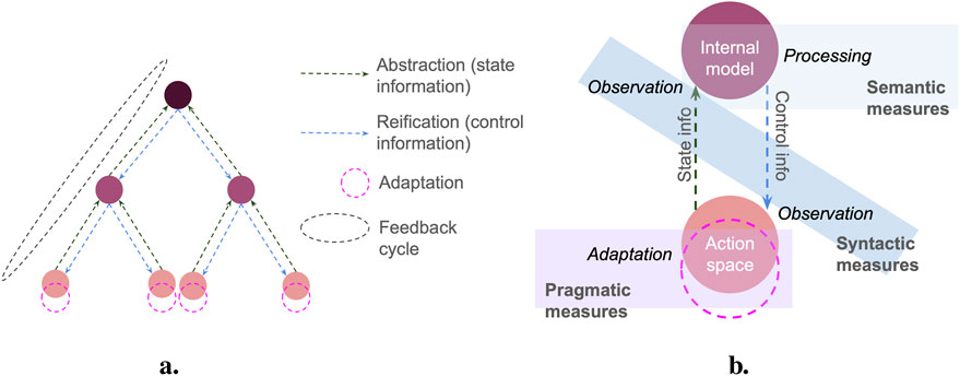
Figure 1. Main MSFS elements. (a) MSFS across three scales, with a single feedback cycle. (b) Syntactic, semantic, and pragmatic information measure domains

Macro-information can take different forms depending on how it is coupled to its physical substrate.

$•$ Exogenous or endogenous. Exogenous macro-information uses a substrate that is external to the substrate of the micro-information sources. The macro-substrate can be another agent—such as a manager collecting information from its workers—or it can be an entity within the environment—for example, a public blackboard showing relevant information to investors or an anthill providing information to ants. Endogenous macro-information uses the same substrate as the micro-information sources. Micro-agents act based on their internal model of an abstract entity in the world, such as members of a society acting based on informal norms governing the group.

$•$ Centralized or distributed. Centralized macro-information uses a substrate that is monolithic, based on tightly coupled components, which are either static or change together as a whole, like managers, pheromone trails, or anthills. Distributed substrates consist of components that are loosely coupled or that change or move independently.

$•$ Structural or symbolic. We use the distinction proposed by Feistel and Ebeling (2016). Structural macro-information is tightly coupled to the structure of its substrate—for example, the size of a bird flock or a bee hive that may impact individual bird or bee behavior. Symbolic macro-information is loosely coupled to the structure of its substrate. It may be encoded differently onto various substrates and decoded by observers accordingly—for instance, managers issuing orders verbally, via email, or through written documents.

The above macro-categories allow for a broad range of CAS to be described as MSFS, with the underlying mechanism being a feedback cycle connecting a minimum of two scales and with the micro-scale adapting based on macro-information.

The abstraction of information allows for CAS that follow an MSFS architecture to scale (Diaconescu et al., 2019). Generally, MSFS should be dimensioned in terms of number of scales, number of entities per scale, and number of inter-entity connections to avoid communication bottlenecks between entities and storage and processing bottlenecks within entities. For example, if an entity receives too much information relative to its resources, the entity should be replicated, with each replica receiving only part of the initial information flow and with an extra, higher-scale entity observing and coordinating these replicas. This can be achieved for all entity macro-types described above. Figure 1b shows the adaptation of a micro-agent with respect to macro-information. The micro-agent is connected to the scales above and below by a flow of state information going upward and control information going downward. Additional flows may exist (e.g., communication among micro-agents). The transmission and observation of these information flows are described by syntactic information measures. When an agent processes information, it may subsequently change its knowledge (its internal model or the output generated by that model) and the action it generates. Processing can happen at different scales. Figure 1b shows a macro-agent processing information and sending the ensuing control information. The micro-agent could also observe the macro-information and process it for its adaptation. The impact of the information flow on an agent’s knowledge is measured by semantic information measures. Changes in the resulting action are measured by pragmatic information measures. Both types of measure can be assessed for one or multiple agents for a single scale or the whole system. Their estimation helps correlate the effects of observed information on knowledge and action with the agent’s (or system’s) adaptation dynamics toward the goal(s).

3.2 Information measures

Information values are observer-dependent (Brillouin, 1953). To measure them, the purpose of the information flow needs to be specified. This can be system viability (Kolchinsky and Wolpert, 2018) or utility toward a goal. In general, value is measured by comparing how the system performs toward a goal state with and without information (Gould, 1974). As all elements in a CAS are informational, various comparison scenarios can be developed. For MSFS, the impact of feedback cycles on agents’ knowledge and actions is calculated by comparing the system at different times. The relevant gap for comparison, depending on the application, can be a single time-step, a single feedback cycle, or multiple cycles. We define the time at which the information measure is calculated as $t$, the previous time used for comparison as $t-\theta$, and the information flowing between $t$ and $t-\theta$ as $I^{t-\theta \to t}$.

We provide general guidelines for the calculation of information measures, to be tailored via specific equations to each domain and case study. There are three steps in the construction and interpretation of information values. First, the system state at time $t$ is assigned a state value with respect to a goal state. These may be knowledge or action states. The state value measures how valuable the state at time $t$ is with respect to the goal state. Depending on the system, this may include how likely it is for the system to reach its goal and/or stay at that goal within a certain timeframe. Then, the state values of the system at times $t$ and $t-\theta$ are compared to measure the impact of $I^{t-\theta \to t}$. Finally, information values for different system configurations are compared to contextualize their dependencies—for example, varying the system architecture, algorithms, or adding errors to $I^{t-\theta \to t}$. In addition to information values, descriptive information measures can be calculated, not taking state values into account. We propose the following information values and descriptive measures:

$•$ The syntactic information content $(C_{\mathit{syn}})$ measures the amount of information in $I^{t-\theta \to t}$. During the feedback cycle, information flows are transmitted, stored, and processed, and $C_{\mathit{syn}}$ estimates the amount of resources needed for this. It can be calculated using Shannon entropy $H$, if probability distributions are known. It can also be calculated using Kolmogorov complexity, the amount of memory used to hold information, or other meaningful proxies of resource use. $C_{\mathit{syn}}$ can be calculated for individual variables, a whole scale, or a full feedback cycle $(C_{\mathit{syn,cycle}})$.

$•$ The semantic information content $(C_{sm})$ is the subset of $C_{\mathit{syn}}$ that has meaning for the agent(s) observing the information. If all $C_{\mathit{syn}}$ can be interpreted, $C_{sm}=C_{\mathit{syn}}$.

$•$ The semantic delta $({\mathrm{\Delta }}_{sm})$ is a descriptive measure that quantifies the magnitude of change in the knowledge due to $I^{t-\theta \to t}$, irrespective of the goal. It can be split into sub-measures depending on which aspects of the knowledge are relevant.

$•$ The semantic truth value $(V_{sm,th})$ measures whether $I^{t-\theta \to t}$ brings the knowledge closer to an observable ground truth $(th)$. First, ground truth state values $S{V}_{th}$ are assigned at times $t$ and $t-\theta$ considering how valuable the knowledge is with respect to ground truth $th$. The calculation of $S{V}_{th}$ depends on the system but usually includes a delta of truth ${\mathrm{\Delta }}_{th}^t$—the distance between the knowledge and $th$ at $t$. $V_{sm,th}$ is then calculated based on the distance between $S{V}_{th}$ at times $t$ and $t-\theta$:

$V_{sm,th}^{t-\theta \to t}=S{V}_{th}^t-S{V}_{th}^{t-\theta }(1)$

$•$ The semantic goal value $(V_{sm,gl})$ measures whether $I^{t-\theta \to t}$ brings the knowledge closer to the optimal knowledge $opt$ needed to reach the goal. This may or may not be the same as the ground truth, depending on the CAS. First, optimal knowledge state values $S{V}_{\mathit{opt}}$ are calculated at $t$ and $t-\theta$. This includes ${\mathrm{\Delta }}_{\mathit{opt}}^t$—the distance at $t$ between knowledge and $opt$. Then, $V_{sm,gl}$ is calculated as the difference between $S{V}_{\mathit{opt}}$ at $t$ and $t-\theta$:

$V_{sm,gl}^{t-\theta \to t}=S{V}_{\mathit{opt}}^t-S{V}_{\mathit{opt}}^{t-\theta }(2)$

$•$ The pragmatic delta $({\mathrm{\Delta }}_{pr})$ is a descriptive measure that quantifies the magnitude of change that $I^{t-\theta \to t}$ has generated on the adaptation. Like ${\mathrm{\Delta }}_{sm}$, it can be divided into sub-measures depending on the relevant adaptation aspects.

$•$ The pragmatic goal value $(V_{pr,gl})$ measures whether the adaptation following $I^{t-\theta \to t}$ brings the system closer to its goal. Goal state values $S{V}_{gl}$ are calculated at $t$ and $t-\theta$, usually requiring the calculation of a ${\mathrm{\Delta }}_{gl}^t$, which is the distance at $t$ between the system state and the goal. $V_{pr,gl}$ represents the change in $S{V}_{gl}$ between $t$ and $t-\theta$:

$V_{pr,gl}^{t-\theta \to t}=S{V}_{gl}^t-S{V}_{gl}^{t-\theta }(3)$

$•$ Efficiencies of each measure can be calculated by dividing it by the $C_{\mathit{syn}}$ of $I^{t-\theta \to t}$.

These guidelines can be used to generate specific equations for different case studies and domains. The exact calculations of each measure and its units depend on the system, as we will show through our four case studies. Moreover, not all measures are relevant to every system—for instance, it may not be possible to identify a ground truth for $V_{sm,th}$. Our measures differ in certain cases from the existing literature. While some authors argue that data need to be contingently true to be considered information (Floridi, 2005; Fetzer, 2004), $V_{sm,th}$ measures whether the information flow has brought knowledge closer or further away from the truth, considering it to have value in both cases. We do not measure pragmatic value as the product of novelty and confirmation, since in our framework both of these refer to the semantic category. If confirmation is zero, then the $C_{sm,cycle}$ of the information is zero, leading to all other semantic and pragmatic measures also being zero. If novelty is zero, however, the information flow may still carry semantic value since it can lead to an update of the agent’s internal model. Efficiencies, then, connect the values to the physical substrates. Considering the example proposed by Frank (2003), while the pragmatic measures would be the same for two different maps leading to the same route, their efficiencies would differ, as they would require different amounts of resources to be processed.

4 Case studies

4.1 Overview

Figure 2 shows a multi-scale representation of the four case studies: robotic collective (RC) (2a), collective decision-making (CD) (2b), task distribution (TD) (2c), and hierarchical oscillators (HO) (2d).

Figure 2

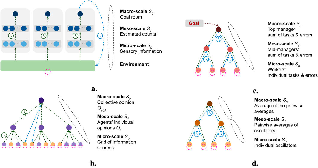
Figure 2. Multi-scale representation of the four case studies. (a) Robotic collective; (b) collective decision-making; (c) task distribution; (d) hierarchical oscillators. Green arrows show abstracted flows of state information, blue arrows show flows of control information, and pink dotted circles show the adaptation. Clocks (blue or green) denote which flows have a delay. In (b), the macro-scale sends control information to each micro-scale agent—only two flows are shown for simplicity. Similarly in (a), where each gray box represents an individual robot, only one flow connecting the robot to the environment is shown.

4.1.1 Robotic collective multi-scale overview

The RC model (Figure 2a) is based on the simulation of a swarm of robots that self-distribute across multiple rooms in proportion to the amount of collectible objects in each room, as in Zahadat (2023). Each robot acts as a micro-agent equipped with sensors that provide it with the lowest scale of information related to the number of robots and objects in the rooms based on the sensing of the environment; this forms the micro-scale $(S_0)$. Over time, robots abstract their micro-scale information into the meso-scale $(S_1)$, consisting of estimations correlated with the current number of robots and objects in the rooms. This is further abstracted into robots’ estimations of each room’s demand for robots, constituting the system’s macro-scale $S_2$. Based on that, the robots decide their motions, forming a feedback loop. The system dynamics are simulated in discrete time steps, and the robots are synchronized: at each time step, all robots update their information at every scale, starting with $S_0$ and ending with $S_2$, followed by a motion action. The process of abstracting micro- into meso-information occurs over time. In contrast, the abstraction of meso- into macro-information happens in a single step. Robots’ motions also unfold over time. As a result, feedback cycles are inseparable from each other, extended in time, and occur at variable intervals depending on the system’s state. We present our measurements either at consecutive timesteps or over a series of intervals.

4.1.2 Collective decision-making multi-scale overview

The CD model simulates a system in which a group of agents makes a collective decision about the size of two tasks by observing their environment. The environment is composed of a fixed set of information sources, each showing one of the two tasks: $A$ and $B$. This is the micro-scale $(S_0)$. Agents are placed on the grid of information sources and each agent forms an individual opinion $O_i$ about the relative size of $A$ by observing the environment around them and averaging what they see. The meso-scale $S_1$ is formed by the set of individual agent opinions. In the second abstraction step, agents go through a consensus process to form a collective opinion $O_{\mathit{coll}}$ of the size of $A$, constituting the macro-scale $S_2$. Then, $O_{\mathit{coll}}$ generates feedback on the micro-scale—that is, the environment of information sources. If agents underestimate the size of $A$, the task will grow until the next feedback cycle, and vice versa. If task $A$ becomes too big or too small, the environment collapses. The goal of the system is to avoid collapse for as long as possible. Timing is discrete: the environment of information sources $(S_0)$ changes at each timestep, and the length of the feedback cycle depends on the system variables and algorithms. We focus on measuring the value of the amount of information used by agents to observe their immediate environment, the number of agents scanning the environment, and the algorithm used to reach a consensus.

4.1.3 Task distribution multi-scale overview

This system aims to distribute a set of tasks of two types across a set of workers. We consider a small system with three scales for traceability reasons (Figure 2c). Larger instances were presented elsewhere (Diaconescu et al., 2021a). At the micro-scale $(S_0)$, workers select an active task of one of two types. The initial choice is random, and then it is driven by feedback from the upper scale $(S_1)$. Managers at the meso-scale $(S_1)$ collect, aggregate, and forward workers’ task choices to the macro-scale $(S_2)$ and then retrieve, split, and distribute the feedback from the macro-scale $(S_2)$ to the workers $(S_0)$. The top manager (at $S_2$) receives the task distribution goal as initial input and provides feedback to the meso-scale $(S_1)$ about the difference between the goal and the workers’ current task choices. Information processing and transmission at each scale depend on the task distribution strategy employed in the system. This forms a feedback cycle $c$, taking two simulation steps. The workers’ state information is sent to the top in one step and then feedback returns one scale at each step. As soon as meso-managers detain new control information, workers adapt to it and send their new states up. Hence, there is a two-step delay between workers sending their state $(t_i)$ and adapting to feedback obtained from that state $(t_{i+2})$. We calculate information measures at each step $t_i$ considering the information flows over the preceding feedback cycle from $t_{i-2}$ to $t_i$.

4.1.4 Hierarchical oscillators multi-scale overview

The HO case study simulates a system of communicating oscillators whose goal is to achieve synchronized oscillation. This system is based on the differential equation model for coupled biochemical oscillators presented in Kim et al. (2010), extended to a hierarchical structure (Mellodge et al., 2021). A single oscillator consists of two interacting components $X$ and $Y$ (e.g., mRNA and protein) in which $X$ inhibits its own synthesis while promoting that of $Y$, and $Y$ inhibits its own and $X$’s synthesis, resulting in a feedback relationship within a single oscillator that induces oscillations in the concentrations of both $X$ and $Y$. In the HO system, multiple scales of oscillators communicate by means of their $X$ concentrations. The oscillators at the micro-scale $S_0$ send their $X$ concentrations to the oscillators at the meso-scale $S_1$ which average that information. These oscillators in turn send their $X$ concentrations to the next highest scale until the macro-scale $S_{M-1}$ is reached, which contains the average of all micro-scale $X$ concentrations. Information is also passed down the system one scale at a time through feedback. The control information contains time-delayed $X$ concentration averages. At each scale $S_m$, oscillators update their own $X$ and $Y$ concentrations based on a combination of current averages from the lower scale $S_{m-1}$ and time-delayed averages from the higher scale $S_{m+1}$. Information measures are used to compare the behavior and performance of two system structures: a two-scale and a three-scale hierarchy.

4.2 Robotic collective

This case study is based on Zahadat (2023), where a homogeneous robotic swarm is designed to self-distribute across four interconnected rooms proportional to the quantity of collectible objects in each room. The four-room layout forms a ring, with each room connected to two others. Here, 200 collectible objects are distributed across four rooms, with 70 objects in each of the first two rooms and 30 in each of the remaining two rooms. The robotic swarm, consisting of 100 robots, is initially distributed uniformly across all rooms. The robots can only detect objects beneath their circular bodies, and their communication range with other robots is twice their diameter. The robots are autonomous and use a variation of the response threshold algorithm (Theraulaz et al., 1998) to independently decide in which room they want to belong: their goal room. The decision is regularly updated based on the robot’s internal model of the environment’s state. Each robot models only the state of the current room and the two rooms connected to that, collectively called the robot’s relevant rooms. The locomotion behavior of the robots is a collision-avoiding random walk, modulated by the current and the goal room: robots can cross room boundaries freely unless they are in their goal room.

We consider the multi-scale feedback generated by the information flowing through the robots’ internal processing structures and feeding back to them via the environment (Figure 2a). $S_0$ consists of information collected through sensory inputs from physical interactions with the outside world. This includes detecting other robots, detecting objects, and receiving communications from other robots. $S_1$ information is an abstraction of micro-information into estimated counts which are approximations designed to correlate with actual counts and are represented as a vector ${\widehat{v}}^t(i)$ for each robot $i$ at time $t$. The vector consists of six components: the first three, ${\widehat{v}}_j^t(i)$ for $j=\mathrm{1,2,3}$, are the estimated object counts in the robot’s three relevant rooms; the last three components, ${\widehat{v}}_{j+3}^t(i)$ for $j=\mathrm{1,2,3}$, are the estimated robot counts in those same rooms. To compute the estimated counts, micro-information is first integrated into sense- and communication-based quantities over time (Zahadat, 2023). Sense-based quantities are calculated as a simple moving average of the number of detections of a robot (or object) over the past $M$ time-steps in each relevant room, where $M$ is the sensing horizon. Communication-based quantities are computed as exponential moving averages of the estimated counts received from other robots. These quantities are then averaged pairwise and normalized across rooms to form ${\widehat{v}}^t(i)$. In $S_2$, the ${\widehat{v}}^t(i)$ is processed to decide on the robot’s goal room. First, a representation of estimated demand for each relevant room is computed:

${\widehat{\phi }}_j^t\left(i\right)={\widehat{v}}_j^t\left(i\right)/\left({\widehat{v}}_j^t\left(i\right)+{\widehat{v}}_{j+3}^t\left(i\right)\right),\text{\hspace{0.17em}for\hspace{0.17em}}j=\mathrm{1,2,3}.(4)$

The robot then selects the room with the largest estimated demand as its goal: $g^t(i)=\arg {\max }_{j=\mathrm{1,2,3}}{\widehat{\phi }}_j^t(i)$. A robot’s $g^t(i)$ and whether it matches its current room, influence its locomotion behavior. This can affect the rate of robot exchange between rooms, thereby altering the actual demand in the rooms, which in turn feeds back into the robot’s knowledge system through its sensors.

4.2.1 Comparison strategies

The information processing described above forms our main strategy in this study. We use two configurations for this strategy: main strategy with sensing horizon of $M=100$, and main (short memory) strategy with $M=10$. The two configurations reflect the effects of memory resource usage on the various information measures. In addition to these, two other strategies are implemented: ground truth and random strategies. In both, all processing that leads to the estimated counts is omitted. In the ground truth strategy, the actual counts of robots and objects, normalized across the relevant rooms, are directly copied into the estimated counts.

Comparing the measures between the main and ground truth strategies reflects the effects of the estimation algorithm, particularly regarding sub-optimal accuracy and time delays. In the random strategy, estimated counts are generated by sampling from a uniform distribution, normalized across rooms. Since this strategy lacks feedback loops, it allows us to evaluate the benefits of feedback in achieving the system’s goal.

4.2.2 Information measures

4.2.2.1 Calculations

4.2.2.1.1 Syntactic information

The amount of memory resources that a robot needs to store information at each scale is used as a measure of $C_{\mathit{syn}}$ (detailed in the Supplementary Material). We use ten, $6M+24$, and four memory units in $S_0$, $S_1$, and $S_2$, respectively. The syntactic information content is therefore $C_{\mathit{syn}}^{\mathit{main}}=6M+38$ memory units for the main strategies: $C_{\mathit{syn}}^{\mathit{main}}(M=100)=638$ and $C_{\mathit{syn}}^{\mathit{main}}(M=10)=98$. Since in both ground truth and random strategies the estimated counts are set directly, their syntactic information contents are $C_{\mathit{syn}}^{gt}=C_{\mathit{syn}}^{rn}=10$—six memory units for the estimated counts in $S_1$ and four units used in $S_2$.

4.2.2.1.2 Semantic information

For the semantic delta ${\mathrm{\Delta }}_{sm}$, the change in the knowledge between subsequent time steps is calculated. We first find the absolute change over time for each of the six components of the estimated counts. Since the estimated counts are normalized over the relevant rooms, their values are interrelated. Therefore, we select the largest of the six absolute changes which is then averaged across all robots to obtain the ${\mathrm{\Delta }}_{sm}$ at timestep $t$.

${\mathrm{\Delta }}_{sm}^{\left(t-1\right)\to t}=\frac{1}{N}{\displaystyle \sum _{i=1}^N}\underset{j=1\dots 6}{\max }|{\widehat{v}}_j^{t-1}\left(i\right)-{\widehat{v}}_j^t\left(i\right)|,(5)$

where ${\widehat{v}}^t(i)$ and ${\widehat{v}}^{t-1}(i)$ represent the current and previous estimated counts by robot $i$, and $N$ is the number of robots.

To calculate the semantic truth value $V_{sm,th}$, we first calculate the delta of truth ${\mathrm{\Delta }}_{th}$ after each step, then measure its reduction. The robots’ internal models consist of several sub-models. We consider three: one related to estimated counts at the meso-scale and two related to macro-scale modeling of room demands.

4.2.2.1.2.1 Estimated counts sub-model

We calculate a measure of discrepancy between the estimated and actual counts over time. The estimated count vector ${\widehat{v}}_j^t(i)$ has six elements for each robot $i$ at time $t$. At each timestep, the average of the absolute differences between the estimated and actual counts is taken across the six elements and all robots:

${\mathrm{\Delta }}_{th,counts}^t=\frac{1}{6N}{\displaystyle \sum _{i=1}^N}{\displaystyle \sum _{j=1}^6}\mid {\widehat{v}}_j^t\left(i\right)-v_j^t\mid (6)$

where $v^t$ represents the vector of actual counts.

4.2.2.1.2.2 Highest demand full sub-model

To measure the discrepancy between the internal models and the actual demands, we check whether the demand estimation for the relevant rooms is sufficient to select the room with the highest actual demand as their goal. To quantify this, we calculate the normalized count of robots whose goal room does not match the room with the highest actual demand among the relevant rooms:

${\mathrm{\Delta }}_{th,full}^t=\frac{1}{N}{\displaystyle \sum _{i=1}^N}{\delta }_i^t(7)$

${\delta }_i^t=\left\{\begin{array}{cc}1,\hfill & \text{if\hspace{0.17em}}{g}^t\left(i\right)\ne \arg {\max }_{j=\mathrm{1,2,3}}{\phi }_j^t\left(i\right)\hfill \\ 0,\hfill & \text{else}\hfill \end{array}\right.(8)$

where ${\phi }^t(i)$ represents the actual demands in the relevant rooms for robot $i$ and $g^t(i)$ is the goal of robot $i$ at time step $t$.

4.2.2.1.2.3 Highest demand partial sub-model

When examining the robots’ internal model for estimated demands (data not shown), we observed a strong tendency to identify the local room as having the highest demand. In practice, this means that the robots often choose their local room as their goal and only occasionally target one of the neighboring rooms. The measure here is the same as for the full model but only considers cases where the model does not identify the local room as having the highest demand.

${\mathrm{\Delta }}_{th,partial}^t=\frac{1}{N}{\displaystyle \sum _{i=1}^N}{\delta }_i^t(9)$

${\delta }_i^t=\left\{\begin{array}{cc}1,\hfill & \text{if\hspace{0.17em}}{g}^t\left(i\right)\ne L^t\left(i\right)\text{\hspace{0.17em}and}\hfill \\ \hfill & g^t\left(i\right)\ne \arg {\max }_{j=\mathrm{1,2,3}}{\phi }_j^t\left(i\right)\hfill \\ 0,\hfill & \text{else}\hfill \end{array}\right.(10)$

where $L^t(i)$ represents the local room, ${\phi }^t(i)$ represents the actual demands in the relevant rooms for robot $i$, and $g^t(i)$ is the goal of the robot $i$ at time step $t$.

$V_{sm,th}$ for each of the three sub-models $(V_{sm,th,model}^{t-1\to t}\in [-\mathrm{1,1}])$ and their efficiencies are calculated as

$V_{sm,th,model}^{t-1\to t}={\mathrm{\Delta }}_{th}^{t-1}-{\mathrm{\Delta }}_{th}^t(11)$

$E_{sm,th,model}^{t-1\to t}=\frac{V_{sm,th,model}^{t-1\to t}}{C_{\mathit{syn}}}(12)$

4.2.2.1.3 Pragmatic information

The pragmatic goal value $V_{pr,gl}$ measures whether, at each time step $t$ the distribution of robots across the four rooms, denoted by $r^t$, moves closer to or further away from the desired distribution, denoted by vector $o$. We first calculate the distance between $r^t$ and $o$:

${\mathrm{\Delta }}_{gl}^t=\frac{1}{4}{\displaystyle \sum _{k=1}^4}\mid o_k-r_k^t\mid ,\text{where\hspace{0.17em}}k\in \left\{\mathrm{1,2,3,4}\right\}\text{\hspace{0.17em}is\hspace{0.17em}the\hspace{0.17em}room\hspace{0.17em}number}(13)$

The values ${\mathrm{\Delta }}_{gl}^t\in [\mathrm{0,1}]$ are then used to calculate $V_{pr,gl}$ and efficiencies for given period $\theta$:

$V_{pr,gl}^{t-\theta \to t}={\mathrm{\Delta }}_{gl}^{t-\theta }-{\mathrm{\Delta }}_{gl}^t(14)$

$E_{pr,gl}^{t-\theta \to t}=\frac{V_{pr,gl}^{t-\theta \to t}}{C_{\mathit{syn}}}(15)$

4.2.2.2 Results

The results are pooled from 100 repetitions of independent experimental runs and are presented as the average of all runs, with or without standard deviation for visualization clarity. Figure 3a shows ${\mathrm{\Delta }}_{sm}$ for the two configurations of the main strategy. In both configurations, the knowledge initially undergoes significant changes, driven by the information received at the beginning, which adapts the default knowledge system. After this abrupt initial change, subsequent changes are minor. We also compare the four strategies to determine whether changes in different parts of the knowledge move toward or away from the ground truth they aim to model. Figures 3b–d show the discrepancy between the sub-models and the actual states. As expected, there is no discrepancy between the models in the ground truth strategy. For the random strategy, estimated counts are assigned uniformly at random, and the delta is averaged over the three relevant rooms for each robot, resulting in a constant average discrepancy between the actual and the sub-model counts (Figure 3b). In contrast, the counts for the main strategies initially show an increase in discrepancy, followed by a decrease and eventual stabilization. This initial increase occurs because these strategies cause robots to move between rooms, changing the number of robots in each room. Since these changes take time to be captured in the model, the discrepancy temporarily rises before stabilizing. However, the short memory strategy converges to a slightly higher level of discrepancy. Figures 3c,d show the discrepancies in identifying the room with the highest demand. In both cases, the random strategy performs the worst. After the initial adaptation, the short memory strategy outperforms the long memory strategy for the full model of the relevant rooms (Figure 3c) but performs worse when focusing only on the neighboring rooms (Figure 3d). For both main strategies, the partial models are significantly closer to the ground truth strategy and farther from the random strategy than the full models. This suggests that robots often assume that the current room has the highest demand; otherwise they select the neighboring room with the actual highest demand. Choosing the current room enhances system stability, while selecting the correct neighboring room drives the system toward the desired distribution of robots across rooms. Figure 4 shows the semantic truth values and efficiencies for the three sub-models, highlighting the high fluctuation in the random models across all three cases. A comparison of Figures 4e,f shows higher fluctuations in the full sub-models for the main strategies.

Figure 3

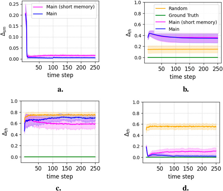
Figure 3. Semantic delta, ${\mathrm{\Delta }}_{sm}^{(t-1)\to t}$ calculated using Equation 5 is shown in (a). The delta to truths for the three model components, ${\mathrm{\Delta }}_{\mathit{\text{th, counts}}}^t$, ${\mathrm{\Delta }}_{\mathit{\text{th, full}}}^t$, ${\mathrm{\Delta }}_{\mathit{\text{th, partial}}}^t$, are calculated using Equations 6, 7, and 9, and shown in (b), (c), (d) respectively.

Figure 4

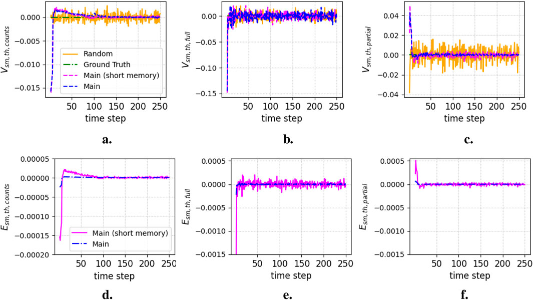
Figure 4. Semantic truth values (Equation 11) and efficiencies (Equation 12) for the three model components. (a) $V_{sm,th,counts}^{t-1\to t}$ (b) $V_{sm,th,full}^{t-1\to t}$ (c) $V_{sm,th,partial}^{t-1\to t}$ (d) $E_{th,counts}^{t-1\to t}$ (e) $E_{th,full}^{t-1\to t}$ (f) $E_{th,partial}^{t-1\to t}$.

Figures 5, 6 compare the pragmatic measures. Figure 5 shows the distance between the actual and desired distributions of robots across the rooms. The random strategy performs the worst, while the main strategy with the long memory achieves the best performance, followed by the short memory strategy. The ground truth strategy performs worse than the main strategies, despite relying on precise models. This is likely due to movement delays, causing late overreactions to perceived issues. This suggests a lack of critical models, possibly related to the spatial organization of robots and their interactions within rooms, which are essential for effective coordination but remain inaccessible to the robot. In contrast, the main strategies demonstrate that partial and imprecise information distributed across robots, rather than attempting an unattainable complete model, leads to better collective behavior.

Figure 5

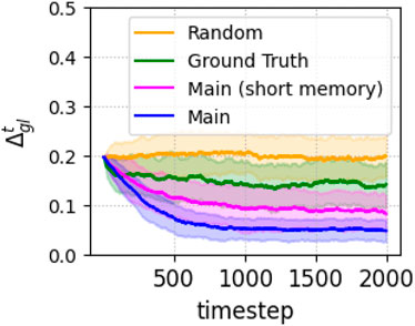
Figure 5. Pragmatic delta (Equation 13) of the various strategies.

Figure 6

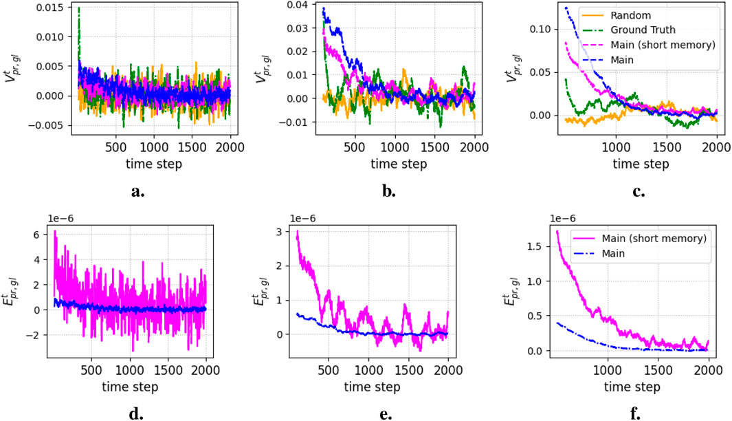
Figure 6. Pragmatic goal values (Equation 14) and efficiencies (Equation 15) of the various strategies. (a) $V_{pr,gl}^{t-10\to t}$ (b) $V_{pr,gl}^{t-100\to t}$ (c) $V_{pr,gl}^{t-500\to t}$ (d) $E_{pr,gl}^{t-10\to t}$ (e) $E_{pr,gl}^{t-100\to t}$ (f) $E_{pr,gl}^{t-500\to t}$.

Figures 6a–c depict the extent to which the robots’ distribution in the rooms approaches the desired distribution over periods of 10, 100, and 500 timesteps. This indicates a pattern similar to that in Figure 5, with large initial adaptations that subsequently oscillate around zero, stabilizing the system. Figures 6d–f illustrate the efficiencies of the main strategies, highlighting the higher resource efficiency of the short memory strategy, particularly over longer feedback cycles.

4.3 Collective decision-making

4.3.1 Model description

The CD model is partially based on Di Felice and Zahadat (2022). It is a simplified representation of decision-making in small, consensus-based groups ($N<30$, where $N$ is the number of agents), where agents react to their environment to avoid collapse. Agents estimate the size of two tasks, $A$ and $B$. The environment is modeled as a polarized grid of 58 × 58 information sources, each showing task $A$ or $B$, with the sum of $A$ and $B$ remaining fixed. The size of each task is measured by the weight of $A{W}_A\in [0.0,1.0]$, determining the share of total information sources showing task $A$. The feedback cycle includes two abstraction steps. First, agents scan $R$ information sources around them, each showing either 0 (task $B$) or 1 (task $A$) and average them out to form an individual opinion $O_i\in [0.00,1.00]$ of $W_A$, with a memory component between subsequent feedback cycles. Second, agents follow a consensus process to reach a collective opinion $O_{\mathit{coll}}\in [0.00,1.00]$, representing the average of $O_i$. The maximum opinion divergence between agents and the number of agents $N$ determines the consensus time $T_{CN}$. For full details on the decision-making algorithm, see the Supplementary Material.

After $T_{CN}$, $O_{\mathit{coll}}$ generates feedback on the environment $W_A$, which grows at each time step until the next feedback cycle if $O_{\mathit{coll}}<W_A$, and shrinks if $O_{\mathit{coll}}>W_A$. If $W_A$ reaches either 0.10 or 0.90, the environment collapses.

4.3.2 Comparison strategies

We refer to the decision-making strategy described above as the consensus strategy. To evaluate it, we implement three reference strategies, randomizing different abstraction steps: opinion formation, consensus formation, or both.

$•$ The random_OP strategy randomizes opinion formation, where agents form a random $O_i[0.00,1.00]$ without perceiving the environment within one time-step. They then form $O_{\mathit{coll}}$ normally, reaching consensus among those random $O_i$. This reflects the extreme situation where opinions are completely disconnected from the environment.

$•$ The random_CN strategy randomizes consensus, where opinions are formed normally and a random $O_i$ is chosen as $O_{\mathit{coll}}$, with the consensus process taking one time step. This reflects the extreme situation where one agent, not better informed than others, holds an opinion with maximum power.

$•$ The random_TOT strategy randomizes $O_{\mathit{coll}}$, taking one time-step.

Comparing the consensus strategy with random_OP highlights the value of evidence-based opinion formation. Comparison with random_CN shows the advantage of the consensus process once opinions have been formed, and comparison with random_TOT evaluates the usefulness of the entire feedback cycle.

4.3.3 Experiments

Parameters $N$ and $R$ are both varied between [1,30]; the starting $W_A$ is set at 0.6, each simulation is capped at 5,000 timesteps, and 40 simulations are run for each $N$×$R$ combination, leading to 36,000 simulations per strategy and a total of 144,000 simulations. Results show the average value across all simulation runs, including a visual representation of uncertainty ranges, when possible. For each simulation, agents are placed randomly on the inner 50 × 50 information grid at $t=0$, with their position not changing, and the environment $W_A$ changing at each time step. Multiple feedback cycles are executed sequentially until the environment collapses or the maximum time is reached.

Figure 7 shows examples of the main types of behavior that can be observed in each simulation. Figure 8 shows average behaviors over the 36,000 simulations for each strategy. Long-lasting simulations (with $t_{\mathit{avg}}$ = 5,000 timesteps) show two patterns. In the first, $O_{\mathit{coll}}$ follows $W_A$ with some delay, leading to an oscillation of both values (Figure 7a). The general strategy behaves this way when $N<15$ and $3<R<15$ (see darker area in Figure 8e), surviving for 5,000 timesteps. In the second pattern, $O_{\mathit{coll}}$ rapidly oscillates between polarized values, forcing $W_A$ to remain stable with tight oscillations around its starting point of 0.6 (Figure 7d). This is what is observed in the high performance area of random_CN (Figure 8f). Here, $T_{CN}$ is reduced to one time step; the $O_i$ randomly chosen as $O_{\mathit{coll}}$ is either 0 or 1 for $R$ = 1 and is likely to remain so for low $R$, leading to a very fast feedback cycle with drastic fluctuations in $O_{\mathit{coll}}$. In other instances, $W_A$ and $O_{\mathit{coll}}$ both enter an oscillatory behavior, but $W_A$ crashes before $5000t$ (Figure 7b). This can happen in the consensus strategy when a slower feedback cycle cannot keep up with changes in $W_A$. Finally, if $W_A$ does not oscillate, it crashes before $t$ reaches 400 timesteps (Figures 7e–h), as observed in both random_TOT and random_OP.

Figure 7

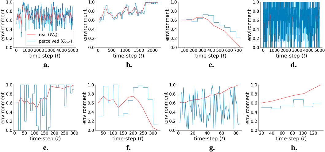
Figure 7. Examples of individual simulations, showing the evolution of $W_A$ and $O_{\mathit{coll}}$ at each time step $t$. (a) Consensus strategy, $N=R=5$; (b) consensus strategy, $N=R=10$; (c) consensus strategy, $N=R=25$; (d) random_CN strategy, $N=R=5$; (e) random_CN strategy, $N=R=10$; (f) random_CN strategy, $N=R=25$; (g) random_TOT strategy, $N=R=10$; (h) random_OP strategy, $N=R=10$. Pink line shows the real environment $(W_A)$; blue line shows the perceived environment $(O_{\mathit{coll}})$.

Figure 8

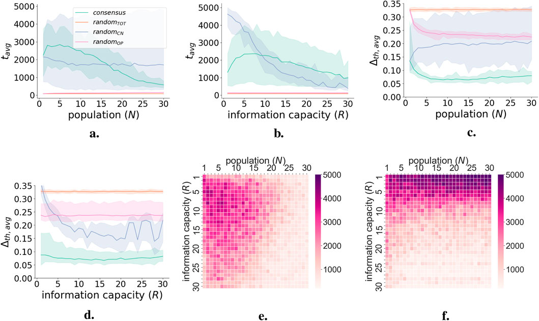
Figure 8. Comparison of average behavior across strategies. (a) Average simulation length ($t_{avg}$) as a function of $N$ for all strategies. (b) Average simulation length ($t_{avg}$) as a function of $R$ for all strategies. (c) Average delta of truth (${\mathrm{\Delta }}_{th,avg}$) as a function of $N$ for all strategies. (d) Average delta of truth (${\mathrm{\Delta }}_{th,avg}$) as a function of $R$ for all strategies. (e) Average simulation length ($t_{avg}$) as a function of $N$ and $R$ for the consensus strategy. (f) Average simulation length ($t_{avg}$) as a function of $N$ and $R$ for the random_CN strategy.

Figures 8c and d show the average delta of truth ${\mathrm{\Delta }}_{th,avg}$—that is, the average difference between $O_{\mathit{coll}}$ and $W_A$—for each parameter combination. A lower ${\mathrm{\Delta }}_{th}$ shows that agents are better at collectively perceiving the environment. The relation between ${\mathrm{\Delta }}_{th}$ and $t_{\mathit{avg}}$ highlights the weight of the timing mechanisms in the model. The consensus strategy has the lowest ${\mathrm{\Delta }}_{th,avg}$, and it decreases and stabilizes as $N$ increases (Figure 8c): poor performance at high $N$ is not due to incorrect $O_{\mathit{coll}}$ but to a long feedback cycle that prevents $W_A$ oscillations. For random_CN, ${\mathrm{\Delta }}_{th,avg}$ is highest for low $R$ and even higher than random_TOT and random_OP (Figure 8d). In this range, high $t_{\mathit{avg}}$ is not the result of a good $O_{\mathit{coll}}$ but of an oscillating $O_{\mathit{coll}}$ that stabilizes $W_A$.

4.3.4 Information measures

4.3.4.1 Calculations

We consider $O_{\mathit{coll}}$ as the knowledge for the semantic measures, which could also be calculated at the scale of the opinions of individual agents $O_i$. For the pragmatic measures, the action taken by the system is the change in the environment $W_A$, and we consider the system goal to be furthest from the points of collapse—$W_A=0.10$ or 0.90. Agents are unaware of how far they are from collapse, aiming instead for their local goal of perceiving their immediate environment. Information values are calculated at the granularity of single feedback cycles, comparing the system at time $t$ with $t$−$c$, where $c$ is the number of time steps in the feedback cycle ending at $t$. Values are averaged across feedback cycles within a simulation and then across simulations within each set of $N$×$R$ parameters. Averages are weighted by the number of feedback cycles in each simulation. The resulting information measures reflect these average values, with a full statistical analysis of those averages being out of our current scope.

4.3.4.1.1 Syntactic information

We calculate the amount of resources needed to store information at the meso-scale $S_1$ of an agent’s individual opinions $O_i$ and at the macro-scale $S_2$ of the group’s collective opinion $O_{\mathit{coll}}$. We do not consider the amount of information in the environment at $S_0$ since this is the same for all strategies. We employ Shannon entropy as a measure of resource use at each scale. The syntactic content is summed across scales for the total $C_{\mathit{syn,cycle}}$. Probabilities are simplified by assuming that each information source is equally likely to show one of the two tasks. For the consensus strategy, this leads to a Shannon entropy of each agent’s individual opinion $H(O_i)$ of

$H\left(O_i\right)=-{\displaystyle \sum _k}p\left(O_{i,k}\right){\log }_{2}p\left(O_{i,k}\right)(16)$

Where $O_{i,k}$ in $K$ is the set of all possible opinions, and $p(O_{i,k})$ is the probability of an opinion being $O_{i,k}$. For the entropy at the scale $S_1$, this is multiplied by the number of agents $N$:

$H\left(S_1\right)=N\ast H\left(O_i\right)(17)$

Similarly, the entropy of $S_2$ is

$H\left(S_2\right)=-{\displaystyle \sum _k}p\left(O_{\mathit{coll,k}}\right){\log }_{2}p\left(O_{\mathit{coll,k}}\right)(18)$

Where $O_{\mathit{coll,k}}$ represents all possible values of $O_{\mathit{coll}}$ given a set of $O_{i,k}$, and $p(O_{\mathit{coll,k}})$ the probability that $O_{\mathit{coll}}$ is $O_{\mathit{coll,k}}$. This leads to a final $C_{\mathit{syn,cycle}}$ of

$C_{\mathit{syn,cycle}}=H\left(S_1\right)+H\left(S_2\right)(19)$

Similar calculations are carried out for the three random strategies; full details are included in the Supplementary Material, as well as graphs showing how $C_{\mathit{syn,cycle}}$ varies with $N$ and $R$ for all strategies.

4.3.4.1.2 Semantic information

For the semantic delta ${\mathrm{\Delta }}_{sm}$, the change in $O_{\mathit{coll}}$ between feedback cycles is calculated. This is a proxy of how stable $O_{\mathit{coll}}$ is

${\mathrm{\Delta }}_{sm}^{t-c\to t}=\mid O_{\mathit{coll}}^{t-c}-O_{\mathit{coll}}^t\mid (20)$

Where $O_{\mathit{coll}}^t$ is $O_{\mathit{coll}}$ at the end of the feedback cycle of length $c$ and $O_{\mathit{coll}}^{t-c}$ at the end of the previous feedback cycle. ${\mathrm{\Delta }}_{sm}\in [0.00,1.00]$, with a larger value reflecting a higher change in $O_{\mathit{coll}}$ across feedback cycles. The semantic truth value $V_{sm,th}$ measures whether the information used at each feedback cycle has brought $O_{\mathit{coll}}$ closer or further away from the environment $W_A$ with respect to the $O_{\mathit{coll}}$ of the previous cycle. First, the delta of truth ${\mathrm{\Delta }}_{th}$ is calculated:

${\mathrm{\Delta }}_{th}^t=\mid O_{\mathit{coll}}^t-W_A^t\mid (21)$

Then ${\mathrm{\Delta }}_{th}^t$ is subtracted across feedback cycles to calculate $V_{sm,th}\in [-\mathrm{1,1}]$:

$V_{sm,th}^{t-c\to t}={\mathrm{\Delta }}_{th}^{t-c}-{\mathrm{\Delta }}_{th}^t(22)$

$V_{sm,th}$ is positive when ${\mathrm{\Delta }}_{th}$ decreases between cycles and negative if it increases. Its efficiency is calculated by dividing the value by $C_{\mathit{syn,cycle}}$.

4.3.4.1.3 Pragmatic information

The pragmatic delta ${\mathrm{\Delta }}_{pr}\in [\mathrm{0,1}]$ measures changes in $W_A$ between feedback cycles:

${\mathrm{\Delta }}_{pr}^{t-c\to t}=\mid W_A^{t-c}-W_A^t\mid (23)$

It is a proxy of how stable the environment is, with a higher value reflecting larger environmental change. The pragmatic goal value $V_{pr,gl}$ measures whether the system has moved closer or further away from the goal between a feedback cycle and the next. For this, the delta of goal ${\mathrm{\Delta }}_{gl}\in [\mathrm{0,1}]$ is calculated at each $t$, with higher values for system states that are further from the point of collapse:

${\mathrm{\Delta }}_{gl}^t=1-2\ast \mid 0.5-W_A^t\mid (24)$

We then calculate $V_{pr,gl}^{t-c\to t}\in [-\mathrm{1,1}]$ as

$V_{pr,gl}^{t-c\to t}={\mathrm{\Delta }}_{gl}^{t-c}-{\mathrm{\Delta }}_{gl}^t(25)$

Similar to $V_{sm,th}$, $V_{pr,gl}$ takes negative values when the system moves closer to collapse relative to the previous feedback cycle, and vice versa.

4.3.4.2 Results

Figure 9 shows the average information measures as a function of $N$ and $R$. We focus on the behavior of the consensus and random_CN strategies that are comparable in terms of $t_{\mathit{avg}}$. ${\mathrm{\Delta }}_{sm}$ and ${\mathrm{\Delta }}_{pr}$ show the evolution of variations in $O_{\mathit{coll}}$ and $W_A$, respectively. For the consensus strategy, there is an overall correlation between $t_{\mathit{avg}}$ (Figure 8e), ${\mathrm{\Delta }}_{sm}$, and ${\mathrm{\Delta }}_{pr}$: higher fluctuations in $W_A$ are associated with a lower $t_{\mathit{avg}}$, which is caused by higher fluctuations in $O_{\mathit{coll}}$. There is an exception for $N$ = 1 (Figure 9a), where $O_{\mathit{coll}}$ oscillates between 0 and 1, leading to a stable environment (Figure 9c). For random_CN, ${\mathrm{\Delta }}_{sm}$ is considerably higher ($O_{\mathit{coll}}$ is unstable), and there are two possible relations between ${\mathrm{\Delta }}_{sm}$, ${\mathrm{\Delta }}_{pr}$, and $t_{\mathit{avg}}$. In the area of low $R$, ${\mathrm{\Delta }}_{sm}$ is high, ${\mathrm{\Delta }}_{pr}$ is low, and $t_{\mathit{avg}}$ is high—$O_{\mathit{coll}}$ fluctuates strongly between one feedback cycle and the next, forcing the environment to stabilize. A different pattern emerges from $R=23$, with bands of high ${\mathrm{\Delta }}_{sm}$ (Figure 9b) also leading to a high ${\mathrm{\Delta }}_{pr}$ and a low $t_{\mathit{avg}}$. In this range, random_CN acts like the consensus strategy, with changes in $O_{\mathit{coll}}$ coupled to a slower feedback cycle, leading to a faster collapse. The discrepancy in values in the range of $R>23$ for random_CN is likely due to noisy results because of the limited sample size; this needs further exploration. Depending on the system, specific combinations of ${\mathrm{\Delta }}_{sm}$, ${\mathrm{\Delta }}_{pr}$, and $t_{\mathit{avg}}$ may be more or less desirable. For example, an $O_{\mathit{coll}}$ that changes in line with $W_A$, leading to stable oscillations (such as when the consensus strategy performs well), may be more desirable than a highly varying $O_{\mathit{coll}}$ that flattens changes in $W_A$ but that may quickly lead to collapse if conditions change.

Figure 9

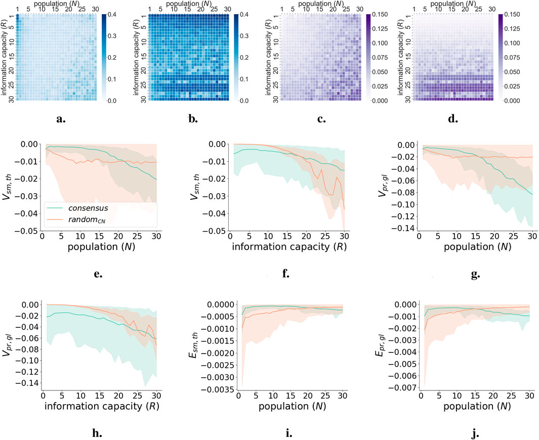
Figure 9. Semantic and pragmatic information measures for collective decision-making case study. (a) Semantic delta ${\mathrm{\Delta }}_{sm}$ of the consensus strategy. (b) Semantic delta ${\mathrm{\Delta }}_{sm}$ of the random_CN strategy. (c) Pragmatic delta ${\mathrm{\Delta }}_{pr}$ of the consensus strategy. (d) Pragmatic delta ${\mathrm{\Delta }}_{pr}$ of the random_CN strategy. (e) Semantic truth value $V_{sm,th}$ for the consensus and random_CN strategies, as a function of N. (f) Semantic truth value $V_{sm,th}$ for the consensus and random_CN strategies, as a function of $R$. (g) Pragmatic goal value $V_{pr,gl}$ for the consensus and random_CN strategies, as a function of $N$. (h) Pragmatic goal value $V_{pr,gl}$ for the consensus and random_CN strategies, as a function of $R$. (i) Efficiency of $V_{sm,th}$ for the consensus and random_CN strategies, as a function of $N$. (j) Efficiency of $V_{pr,gl}$ for the consensus and random_CN strategies, as a function of $N$.

$V_{sm,th}$ and $V_{pr,gl}$ show whether each feedback cycle on average brings $O_{\mathit{coll}}$ closer or further away from $W_A$, and whether $W_A$ moves closer or further away from a desirable state between subsequent cycles. Values are almost entirely negative for both consensus and random_CN (Figures 9e–h), meaning that on average, each feedback cycle has a worse performance than that previous. The exception is for low $R$ in random_CN, where strong fluctuations of $O_{\mathit{coll}}$ keep $W_A$ stable. Stability can also be considered across parameter ranges: while random_CN leads to a stable $W_A$ for low $R$, increasing the range of $R$ quickly leads to instability, while parameter transitions are smoother for the consensus strategy. Efficiencies (9i and 9j) show how for both strategies (and more strongly for random_CN) at low $N$, less information is needed to produce larger (negative) values. Overall, comparison with random_CN provides insights into the value of the consensus process as formalized in this model, with its polarized environment, opinion formation, and consensus algorithms. While it might be better for low $N$ to pick a random agent’s opinion as the prevailing one in terms of $t_{\mathit{avg}}$, the consensus strategy maintains more stability in $O_{\mathit{coll}}$ and a higher $V_{sm,th}$ of the average feedback cycle. The comparison with random_TOT and random_OP, while not explored in detail here, shows that the opinion formation step is essential to the functioning of the model.

4.4 Task distribution

4.4.1 Model description

This model is a simplified version of the ABM in Diaconescu et al. (2021a), aiming to achieve a given task distribution among a set of agents. We exemplify a small system to facilitate the formal analysis of information flows. The system contains $N=3$ scales $S_s$, where $s=02$, populated by agents $a_{s,j}$ at scale $S_s$ and index $j$. $S_0$ includes four workers $(|S_0|=4)$ that must select two task types, $k_0$ and $k_1$ (sometimes noted as 0 and 1), according to given proportions $g_0$, $g_1$, where $g_0+g_1=|S_0|$. Workers coordinate their task selection via managers, each handling $C=2$ children (Figure 2c). At $t_0$, the top-manager $a_{\mathrm{2,0}}$ receives the goal $v_g=g_1$, and workers $a_{0,j}$, where $j=0.4$, are assigned an active task $k_a\in \{k_0,k_1\}$. Time is modeled in discrete steps $t_i$. For simplicity, we only consider information about $k_1$, $k_0$ being complementary to it.

Each manager $a_{s,j}$, $s>0$, holds two variables concerning its children: the number of workers that execute $k_1$ (abstraction $v_{s,j}^A$) that should switch to $k_1$ (control-error $v_{s,j}^{\mathrm{\Delta }}$). For workers, $v_{0,j}^A=v_{0,j}^{k_a}$ (their active task) and $v_{0,j}^{\mathrm{\Delta }}=v_{1,l}^{\mathrm{\Delta }}$ (control from parent $a_{1,l}$).

The system uses the Blackboard (BB) strategy (simplified from Diaconescu et al. (2021a) —see Supplementary Material for further details), forming a multi-scale feedback cycle via the following information flows.

$•$ Abstraction: managers sum up their children states (active tasks), $v_{s,j}^A={\sum }_{c=01}{v}_{s-1,c}^A$

$•$ Processing: the top-manager calculates the error between its abstract state and the goal, $v_{\mathrm{2,0}}^{\mathrm{\Delta }}=v_{\mathrm{2,0}}^A-v_g$, where negative errors indicate that more workers should pick $k_1$.

$•$ Reification: mid-managers fetch the control error $v_{\mathrm{2,0}}^{\mathrm{\Delta }}$ from the top, split it equally between them, and round up the remainder, then send the result to workers $v_{1,j}^{\mathrm{\Delta }}$

$•$ Adaptation: workers that perform $k_a=k_0$ and receive a negative error $v_{1,l}^{\mathrm{\Delta }}<0$ switch to $k_1$ with probability $p_{ch}=0.15$; otherwise they do nothing.

The BB simulation repeats this cycle recursively until the goal is reached, and it is maintained for $N=3$ steps.

4.4.2 Comparison strategies

We define several alternative strategies for reference.

$•$ Random switch (RS): at each step, workers switch states with probability $p_{ch}=0.15$ (same as BB).

$•$ Random blind (RB): at each step, workers switch states randomly, $p_{ch}=0.5$.

$•$ Static (St): workers keep their initial states.

$•$ Model (Md): managers collect detailed information about which worker performs which task and feed back exactly which workers should switch tasks, hence reaching the goal in $N=3$ steps.

We selected these alternative strategies based on the following considerations.

$•$ St provides an extreme case where the system does not adapt, whereas RB provides the other extreme where the system adapts completely randomly.

$•$ RS resembles BB except that it only uses local state information with no higher-scale coordination.

$•$ Md shows how the system adapts when accessing all available information (ground-truth).

4.4.3 Experiments

In the initial state, all workers perform $k_0$ $(v_{S_0}^k=0000)$, whereas the goal $v_g=4$ indicates that they should perform $k_1$ $(v_{g,S_0}^k=1111)$. Experiments rely on an analytic simulation to facilitate information tracking. We employ two experimental alternatives.

$•$ Probabilistic analysis $E{x}_{\mathit{all}}$ for all strategies considers all possible system behaviors over 50 steps. We use this to estimate probabilities for the syntactic content and pragmatic values.

$•$ Concrete scenario, $E{x}_{\mathit{scenario}}$ for BB and Md: illustrates a particular behavior over six steps (see Figure 10 for BB, Supplementary Material for Md). We use this to track semantic and pragmatic delta measures step by step.

Figure 10

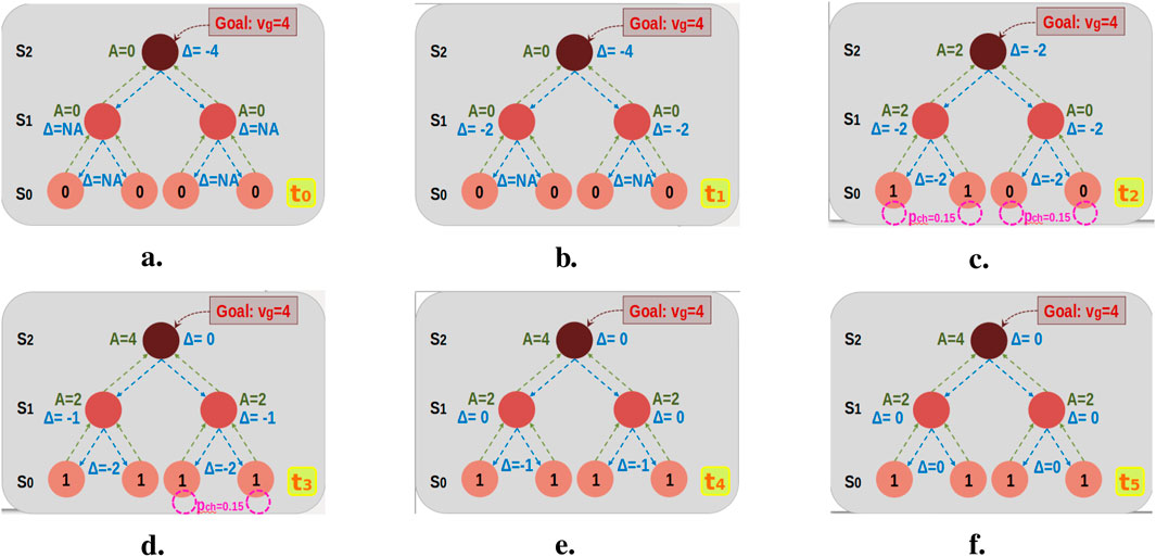
Figure 10. Task-distribution scenario $E{x}_{\mathit{scenario}}$ using the Blackboard (BB) strategy with four workers, two mid-managers, and one top-manager, reaching goal $v_{g,S_0}=1111$ from initial state $v_{S_0}^{t_0}=0000$ in four steps. (a) $t_0$ (b) $t_1$ (c) $t_2$ (d) $t_3$ (e) $t_4$ (f) $t_5$.

4.4.4 Information measures

We define information measures through generic equations and then illustrate them in specific cases. We consider all measures for BB and Md and only syntactic content and pragmatic values for RS, RB, and St, as they lack multi-scale coordination. Table 1 summarizes results for syntactic $(E{x}_{\mathit{all}})$, semantic $(E{x}_{\mathit{scenario}})$, and pragmatic delta $(E{x}_{\mathit{scenario}})$ measures. Figure 11 compares pragmatic values of all strategies $(E{x}_{\mathit{all}})$ (see the Supplementary Material for further results and calculations).

Table 1

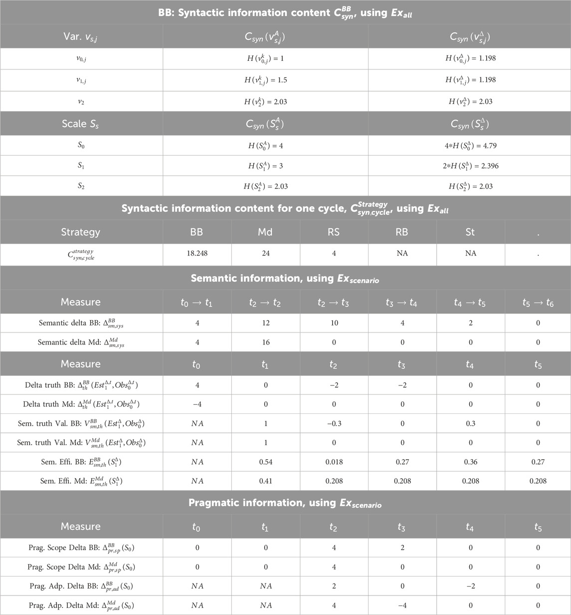
Table 1. Information measures for the task distribution case. Syntactic content and pragmatic values rely on the probabilistic analysis of all possible behaviors via $E{x}_{\mathit{all}}$. Semantic value and pragmatic delta measures are exemplified via $E{x}_{\mathit{scenario}}$.

Figure 11

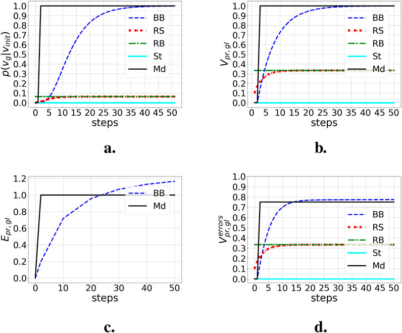
Figure 11. Probabilities of goal convergence and pragmatic goal values within 50 steps from initial state $v_{S_0}^{t_0}=0000$ to goal state $v_g=1111$ for different adaptation strategies. To calculate $V_{pr,gl}^{t_0\to t_{49}}$, we considered state values $S{V}_{gl}(S_0)=\{\mathrm{0,0.25},0.5,0.75,1\}$. (a) Probabilities to reach the goal. (b) Pragmatic goal values with correct info. (c) Efficiency of the pragmatic goal value. (d) Pragmatic goal values with error info.

4.4.4.1 Syntactic information

We estimate the syntactic information content $C_{\mathit{syn}}$ using Shannon entropy $H(\cdot )$ (Diaconescu et al., 2021b) for each agent variable. To provide an upper limit for $C_{\mathit{syn}}$, we consider the workers’ task selections and agents’ variables $v_{s,j}^A$ and $v_{s,j}^{\mathrm{\Delta }}$ as independent. Furthermore, we only distinguish between collective states (at each scale) featuring different task distributions—that is, the same number $z$ of workers performing $k_a=k_1$ regardless of their arrangements. For example, for $z=1$, $v_{S_0}^k\in$ {0001, 0010, 0100, 1000} are equivalent, leading to $v_2^A=1$, $v_2^{\mathrm{\Delta }}=-3$.

For any variable $v_{s,j}$ taking numerical values $va{l}_s\in V_s$ with probabilities $p_{va{l}_s}$, we have

$C_{\mathit{syn}}\left(v_{s,j}\right)=H\left(v_{s,j}\right)={\displaystyle \sum _{va{l}_s\in V_s}}-p_{va{l}_s}\ast lo{g}_2\left(p_{va{l}_s}\right)(26)$

For an entire scale $S_s$, the entropy is the sum of individual entropies of variables $H(v_{s,j})$ if $v_{s,j}$ have different information sources. Otherwise, $H(S_s)$ is the same as $H(v_{s,j})$ for all $j$. This gives

$H\left(S_s\right)=\left\{\frac{{\displaystyle \sum _{j=0}^{|S_s|-1}}H\left(v_{s,j}\right)\text{,\hspace{0.17em}if\hspace{0.17em}}{v}_{s,j}\text{has\hspace{0.17em}different\hspace{0.17em}info\hspace{0.17em}sources\hspace{0.17em}for\hspace{0.17em}each\hspace{0.17em}}j(\text{e.g.\hspace{0.17em}abstraction\hspace{0.17em}from\hspace{0.17em}different\hspace{0.17em}micro}-\text{sources})}{H\left(v_{s,j}\right)\text{,\hspace{0.17em}for\hspace{0.17em}any\hspace{0.17em}}j\text{,\hspace{0.17em}if\hspace{0.17em}all\hspace{0.17em}}{v}_{s,j}\text{\hspace{0.17em}have\hspace{0.17em}the\hspace{0.17em}same\hspace{0.17em}information\hspace{0.17em}source}(\text{e.g.\hspace{0.17em}error\hspace{0.17em}broadcast\hspace{0.17em}from\hspace{0.17em}the\hspace{0.17em}same\hspace{0.17em}macro}-\text{source})}\right.(27)$

We then estimate the amount of information “lost” or “gained” via inter-scale abstraction or reification:

$\mathrm{\Delta }{H}_{S_s\to S_{s+i}}=H\left(S_{s+i}\right)-H\left(S_s\right)(28)$

For example, BB’s abstraction flow loses $25\%$ from $S_0$ to $S_1$ $(\mathrm{\Delta }{H}_{S_0\to S_1}^{BB,A}=-1)$, and further, $\approx 32\%$ from $S_1$ to $S_2$ $(\mathrm{\Delta }{H}_{S_1\to S_2}^{BB,A}=-0.97)$. BB’s control flow also loses $41\%$ of information from $S_2$ to $S_1$ $(\mathrm{\Delta }{H}_{S_2\to S_1}^{\mathrm{\Delta }}\approx -0.8)$, as different error indicators from the top-manager map to the same indicator from mid-managers (e.g., both $v_{\mathrm{2,0}}^{\mathrm{\Delta }}=4$ and 3 are split into $v_{\mathrm{1,0}}^{\mathrm{\Delta }}=v_{\mathrm{1,1}}^{\mathrm{\Delta }}=2$). No information is lost from $S_1$ to $S_0$ as mid-managers broadcast to workers. In contrast, Md loses no information in either state, and it controls flows.

In all cases, resource use depends on the number of variables at each scale:

$C_{\mathit{syn}}\left(S_s\right)={\displaystyle \sum _{j=0}^{|S_s|-1}}{C}_{\mathit{syn}}\left(v_{s,j}\right)(29)$

For BB, the control flow’s resource usage is larger than its information content: $C_{\mathit{syn}}^{BB}(S_s^{\mathrm{\Delta }})>H^{BB}(S_s^{\mathrm{\Delta }})$ (Table 1). It gains $18\%$ in syntactic content from $S_2$ to $S_1$, and $99.9\%$ from $S_1$ to $S_0$.

Finally, we consider the syntactic content of an entire feedback cycle (see Table 1):

$C_{\mathit{syn,cycle}}={\displaystyle \sum _{s=02}}{C}_{\mathit{syn}}\left(S_s^A\right)+{\displaystyle \sum _{s=02}}{C}_{\mathit{syn}}\left(S_s^{\mathrm{\Delta }}\right)(30)$

4.4.4.2 Semantic information

The semantic delta ${\mathrm{\Delta }}_{sm}$ of an agent’s variable $v_{s,j}$ measures changes in its numerical values. For one step, we have

${\mathrm{\Delta }}_{sm}^{t_i\to t_{i+1}}\left(v_{s,j}\right)=|v_{s,j}^{t_{i+1}}-v_{s,j}^{t_i}|(31)$

For the entire system,

${\mathrm{\Delta }}_{sm,sys}^{t_i\to t_{i+1}}={\displaystyle \sum _s}{\displaystyle \sum _j}{\mathrm{\Delta }}_{sm}^{t_i\to t_{i+1}}\left(v_{s,j}\right)(32)$

Using $E{x}_{\mathit{scenario}}^{BB}$ (Figure 10), $t=05$, gives the subsequent measures: ${\mathrm{\Delta }}_{sm,sys}^{BB,t\to t+1}=\mathrm{4,12,10,4,2,0}$ (see full details in Supplementary Material). Hence, BB’s knowledge changes during adaptation $(t=04)$ then stabilizes when the goal is reached $(t\ge 5)$. Md features ${\mathrm{\Delta }}_{sm,sys}^{Md,t\to t+1}=\mathrm{4,16,0,0,0,0}$, indicating larger, more rapid knowledge changes as Md converges more rapidly towards the goal.

We calculate the semantic truth value $V_{sm,th}$ based on three steps. We focus on $V_{sm,th}$ for managers’ control flows to highlight the difference between their knowledge (leading to workers’ adaptation) and the workers’ actual state at $t$.

First, we estimate the delta of truth ${\mathrm{\Delta }}_{th}$ at $t$ as the difference between the managers’ estimated error $Es{t}_s^{\mathrm{\Delta },t}$ and the workers’ actual error to the goal $Ob{s}_0^{\mathrm{\Delta },t}$:

$Es{t}_s^{\mathrm{\Delta },t}={\displaystyle \sum _{j=0}^{|S_s|-1}}{v}_{s,j}^{\mathrm{\Delta },t}\text{,s\hspace{0.17em}}>0(33)$

$Ob{s}_0^{\mathrm{\Delta },t}=v_g-{\displaystyle \sum _{j=0}^{|S_0|-1}}{v}_{0,j}^{k,t}(34)$

${\mathrm{\Delta }}_{th}\left(Es{t}_s^{\mathrm{\Delta },t},Ob{s}_0^{\mathrm{\Delta },t}\right)=Es{t}_s^{\mathrm{\Delta },t}-Ob{s}_0^{\mathrm{\Delta },t}(35)$

We consider ${\mathrm{\Delta }}_{th}=0$ when $Es{t}_s^{\mathrm{\Delta },t}=NA$, $t=01$.

Using $E{x}_{\mathit{scenario}}$, $t=05$, we obtain for BB ${\mathrm{\Delta }}_{th}^{BB}(Es{t}_1^{\mathrm{\Delta },t},Ob{s}_0^{\mathrm{\Delta },t})=\mathrm{4,0},-2,-\mathrm{2,0,0}$ and for Md ${\mathrm{\Delta }}_{th}^{Md}(Es{t}_1^{Md,\mathrm{\Delta },t},Ob{s}_0^{Md,\mathrm{\Delta },t})=-\mathrm{4,0,0,0,0,0}$. These differences are due to communication delays. As above, they occur during the adaptation period (shorter for Md).

Second, we assign values $S{V}_{th}$ to different knowledge states, depending on their distance to the truth:

$S{V}_{th}\left(Es{t}_s^{\mathrm{\Delta },t},Ob{s}_0^{\mathrm{\Delta },t}\right)=1-|\frac{{\mathrm{\Delta }}_{th}\left(Es{t}_s^{\mathrm{\Delta },t},Ob{s}_0^{\mathrm{\Delta },t}\right)}{{\mathrm{\Delta }}_{th,max}}|(36)$

With ${\mathrm{\Delta }}_{th,max}=4$ the maximum ${\mathrm{\Delta }}_{th}$ in our case.

Maximum $S{V}_{th}=1$ indicates no difference to truth, and minimum $S{V}_{th}=0$ the largest difference. This gives, for BB, $S{V}_{th}^{BB}=\mathrm{0,1,0.5},0.5,\mathrm{1,1}$ and for Md, $S{V}_{th}^{Md}=\mathrm{0,1,1,1,1,1}$. We note that, due to delays, $S{V}_{th}$ becomes 1 (highest) when the system undergoes no adaptation and $\le 1$ (lower) otherwise.

Third, we calculate $V_{sm,th}\in [-\mathrm{1,1}]$:

$V_{sm,th}^t\left(Es{t}_s^{\mathrm{\Delta },t},Ob{s}_0^{\mathrm{\Delta },t}\right)=\left\{\begin{array}{c}\mathbf{N}\mathbf{A},if\hspace{0.17em}no\hspace{0.17em}knowledge\hspace{0.17em}of\hspace{0.17em}Es{t}_s\hspace{0.17em}at\hspace{0.17em}t-1\hspace{0.17em}or\hspace{0.17em}t\hfill \\ \frac{S{V}_{kn}\left(Es{t}_s^{\mathrm{\Delta },t-1},Ob{s}_0^{\mathrm{\Delta },t}\right)==NA\vee S{V}_{kn}\left(Es{t}_s^{\mathrm{\Delta },t},Ob{s}_0^{\mathrm{\Delta },t}\right)==NA}{\mathbf{0},if\hspace{0.17em}no\hspace{0.17em}change\hspace{0.17em}from\hspace{0.17em}t-1\text{\hspace{0.17em}to\hspace{0.17em}}t}\hfill \\ \frac{S{V}_{kn}\left(Es{t}_s^{\mathrm{\Delta },t-1},Ob{s}_0^{\mathrm{\Delta },t}\right)==S{V}_{kn}\left(Es{t}_s^{\mathrm{\Delta },t},Ob{s}_0^{\mathrm{\Delta },t}\right)}{\frac{S{V}_{kn,s}^{\mathrm{\Delta },t}-S{V}_{kn,s}^{\mathrm{\Delta },t-1}}{S{V}_{kn,s}^{\mathrm{\Delta },t}+S{V}_{kn,s}^{\mathrm{\Delta },t-1}},otherwise}\hfill \end{array}\right.(37)$

We have $V_{sm,th}^t=0$ (neutral) if knowledge was unavailable at $t$-1 or remained unchanged from $t$-1 to $t$; $V_{sm,th}^t\in (\mathrm{0,1}]$ (positive) if $S{V}_{kn}$ increased (closer to truth), and $V_{sm,th}^t\in [-\mathrm{1,0})$ (negative) if $S{V}_{kn}$ decreased (farther from truth). As before, fluctuations are due to estimation lags and neutral values to stable states.

We estimate the efficiency of the semantic truth value $E_{sm,th}\in [\mathrm{0,1}]$ based on the resources required through a feedback cycle $C_{\mathit{syn,cycle}}$ (Equation 30):

$E_{sm,th}^t\left(S_1^{\mathrm{\Delta }}\right)=\frac{\left(V_{sm,th}\left(Es{t}_{S_1^{\mathrm{\Delta }}}^t,Ob{s}_{S_0^{\mathrm{\Delta }}}^t\right)+1\right)/2}{C_{\mathit{syn,cycle}}}\ast coef(38)$

We normalize $E_{sm,th}$ to fit the interval [0,1] and to indicate better efficiency for higher $V_{sm,th}$ and lower $C_{\mathit{syn,cycle}}$, and worse efficiency for worse $V_{sm,th}$ and higher $C_{\mathit{syn,cycle}}$. We employ a scaling factor $coef=10$ for readability reasons. We note that BB features $\approx 31.5\%$ better efficiency than Md for the same $V_{sm,th}$ values, as Md uses $\approx 31.5\%$ more resources than BB.

4.4.4.2.1 Pragmatic information

We focus on evaluating how mid-managers’ control of information $v_{S_1}^{\mathrm{\Delta }}$ influences workers’ adaptations $K_{\mathit{act}}(S_0)$ toward the goal $v_g$.

We consider two types of pragmatic delta ${\mathrm{\Delta }}_{pr}$ for worker changes.

$•$ Pragmatic scope delta ${\mathrm{\Delta }}_{pr,sp}$: changes in the scope of possible adaptations $|K_{\mathit{act}}|$.

$•$ Pragmatic adaptation delta ${\mathrm{\Delta }}_{pr,ad}$: changes in the magnitude of actual adaptations $|K_{ch}|$.

The pragmatic scope delta ${\mathrm{\Delta }}_{pr,scp}$ measures how the number of adaptation actions $|K_{\mathit{act}}(S_0)|$ changes when workers receive $v_{S_1}^{\mathrm{\Delta }}$ or not:

${\mathrm{\Delta }}_{pr,sp}^t\left(S_0\right)={\displaystyle \sum _{j=0}^3}\left(|K_{\mathit{act}}^{t,inf}\left(a_{0,j}\right)|-|K_{\mathit{act}}^{t,noInf}\left(a_{0,j}\right)|\right)(39)$

In BB and Md, workers may only switch tasks when receiving control information; otherwise they stay idle. Hence, no information implies $|K_{\mathit{act}}^{t,noInf}(a_{0,j})|=0$, and received information implies $|K_{\mathit{act}}^{t,inf}(a_{0,j})|=1$ if the worker switches, and $|K_{\mathit{act}}^{t,inf}(a_{0,j})|=0$ otherwise. Positive ${\mathrm{\Delta }}_{pr,sp}$ means that information increases the number of potential adaptations, and negative ${\mathrm{\Delta }}_{pr,sp}$ that it reduces them.

In $E{x}_{\mathit{scenario}}$, $t=05$, we have ${\mathrm{\Delta }}_{pr,scp}^{BB}(S_0)=\mathrm{0,0,4,2,0,0}$. These correspond to workers’ potential adaptations at $t_2$ and $t_3$ (see pink circles in Figures 10c,d). For Md, we have $V_{pr,scp}^{Md}(S_0)=\mathrm{0,0,4,0,0,0}$, indicating that all adaptations occur at $t=2$.

The pragmatic adaptation delta ${\mathrm{\Delta }}_{pr,ad}$ measures actual adaptation differences between $t-1$ and $t$:

${\mathrm{\Delta }}_{pr,adp}^t\left(S_0\right)={\displaystyle \sum _{j=0}^3}\left(|K_{ch}^t\left(a_0,j\right)|-|K_{ch}^{t-1}\left(a_0,j\right)|\right)(40)$

Here, $|K_{ch}(a_{0,j})|=1$ if worker $a_{0,j}$ switches tasks, and $|K_{ch}(a_{0,j})|=0$ otherwise.

In $E{x}_{\mathit{scenario}}$, $t=05$, we have ${\mathrm{\Delta }}_{pr,adp}^{BB,t}=NA,NA,\mathrm{2,0},-\mathrm{2,0}$ and ${\mathrm{\Delta }}_{pr,adp}^{Md,t}=NA,NA,4,-\mathrm{4,0,0}$. This indicates that adaptation happens progressively for BB ($t_2$ and $t_3$) and all at once for Md $(t_2)$.

We estimate the pragmatic goal value $(V_{pr,gl})$ of information based on the likelihood that strategies bring the task distribution toward the goal $v_g$. We calculate $V_{pr,gl}$ in three steps, as follows.

$•$ Assign a state value $S{V}_{gl}(v_{S_0}^k)$ to each task-distribution state $v_{S_0}^k$.

$•$ Assign a pragmatic adaptation value $V_{pr,ad}(v_{S_0}^k)$ to each state, based on its potential to adapt into more valuable states (closer to the goal).

$•$ Calculate the pragmatic goal value $V_{pr,gl}(v_{S_0}^k)$ based on the above adaptation value, current state value, and ability to maintain the goal once reached.

We assign state values $S{V}_{gl}\in [\mathrm{0,1}]$ to different task distribution groups $S_0^z$ ($z$ the number of workers executing $k_1$) depending on their distance from $v_g$. $S{V}_{gl}=1$ is the highest value (goal reached) and 0 the lowest. Concretely, we set $S{V}_{gl}(S_0)=\{\mathrm{0,0.25},0.5,0.75,1\}$, meaning that $S{V}_{gl}(S_0^0)=0$, $S{V}_{gl}(S_0^1)=0.25$, $S{V}_{gl}(S_0^2)=0.5$, $S{V}_{gl}(S_0^3)=0.75$, and $S{V}_{gl}(S_0^4)=1$.

We evaluate the pragmatic adaptation value $V_{pr,ad}\in [\mathrm{0,1}]$ based on the workers’ probability to adapt from their present state $v_{S_0}^{k,t}\in V_{S_0}$ to all possible states $v_{S_0}^{w,t+m}\in V_{S_0}$ within $m$ steps. We weight this state-transition probability $p(v_{S_0}^{w,t+m}|v_{S_0}^{k,t})$ by the state value $S{V}_{gl}$ of each adapted state $v_{S_0}^w$. This gives

$V_{pr,ad}^{t\to t+m}\left(v_{S_0}^k\right)={\displaystyle \sum _{v_{S_0}^w:V_{S_0}}}S{V}_{gl}\left(v_{S_0}^w\right)\ast p\left(v_{S_0}^{w,t+m}|v_{S_0}^{k,t}\right)(41)$

We start from state $v_{S_0}^0=0000$ and aim for $v_g=1111$. Thus, state-transition probabilities are the likelihood that workers switch from $k_0$ to $k_1$ at each step (for details, see Supplementary Material). For BB, this gives the stochastic matrix $M$ for one step, with states $S_0^z\in \{\mathrm{0000,0001,0011,0111,1111}\}$ from left to right (columns) and top-down (rows):

$M=\left[\begin{array}{ccccc}\hfill 0.522\hfill & \hfill 0.3684\hfill & \hfill 0.0975\hfill & \hfill 0.0114\hfill & \hfill \mathbf{0.0005}\hfill \\ \hfill 0\hfill & \hfill 0.6141\hfill & \hfill 0.3251\hfill & \hfill 0.0573\hfill & \hfill 0.0034\hfill \\ \hfill 0\hfill & \hfill 0\hfill & \hfill 0.723\hfill & \hfill 0.255\hfill & \hfill 0.0225\hfill \\ \hfill 0\hfill & \hfill 0\hfill & \hfill 0\hfill & \hfill 0.85\hfill & \hfill 0.15\hfill \\ \hfill 0\hfill & \hfill 0\hfill & \hfill 0\hfill & \hfill 0\hfill & \hfill 1\hfill \end{array}\right](42)$

The likelihood that BB reaches the goal in one step is 0.0005. We can then obtain state-transition probabilities over $m$ steps via $M^m={\prod }_{m}M$. Figure 11a shows the probabilities of reaching the goal in $m=050$ steps (cf. Supplementary Material for corresponding $V_{pr,adp}$ values and calculations).

Finally, we assess the pragmatic goal value $V_{pr,gl}\in [-\mathrm{1,1}]$ considering progress between the current state’s value $S{V}_{ds}(v_{S_0}^k)$ and its pragmatic adaptation value $V_{pr,adp}(v_{S_0}^k)$ and the system’s ability to maintain the goal $V_{pr,adp}(v_g)$:

$\begin{array}{cc}\hfill & V_{pr,gl}^{t\to t+m}\left(v_{S_0}^k\right)=\frac{V_{pr,adp}^{t\to t+m}\left(v_{S_0}^k\right)-S{V}_{gl}\left(v_{S_0}^k\right)}{p_{\mathit{goal-keep}}}\hfill \\ \hfill & p_{\mathit{goal-keep}}=\left\{\begin{array}{c}2-V_{pr,adp}^{t\to t+m}\left(v_g\right)\text{,\hspace{0.17em}if\hspace{0.17em}}{V}_{pr,adp}^{t\to t+m}\left(v_{S_0}^k\right)\ge S{V}_{gl}\left(v_{S_0}^k\right)\hfill \\ V_{pr,adp}^{t\to t+m}\left(v_g\right)\hspace{1em}\text{,\hspace{0.17em}if\hspace{0.17em}}{V}_{pr,adp}^{t\to t+m}\left(v_{S_0}^k\right)<S{V}_{gl}\left(v_{S_0}^k\right)\hfill \end{array}\right.\hfill \\ \hfill & \text{considering\hspace{0.17em}}{V}_{pr,gl}^{t\to t+m}\left(v_{S_0}^k\right)=-1\text{\hspace{0.17em},\hspace{0.17em}if\hspace{0.17em}}{p}_{\mathit{goal-keep}}==0\hfill \end{array}(43)$

The maximum value $V_{pr,gl}^{t\to t+m}(v_{S_0}^k)=1$ occurs when the system is sure to reach $v_g$, from the least valuable state, within $m$ steps and then maintain it, $V_{pr,adp}^{t\to t+m}(v_g)=1$. Minimum value $-1$ occurs when the system is sure to regress from $v_g$ to the least valuable state.

Using $E{x}_{\mathit{all}}$, Figure 11b compares $V_{pr,gl}$ results for different strategies over $m=050$ steps. BB has a low pragmatic goal value $V_{pr,gl}^{BB}\approx 0.15$ for $m=1$, yet this increases to $\approx 0.72$ at $m=10$, $\approx 0.94$ at $m=20$, and $\approx 0.98$ at $m=30$. As BB maintains the goal and the initial state value is $S{V}_{ds}(0000)=0$, we have $V_{pr,gl}^{BB}=V_{pr,adp}^{BB}$, $\forall m$. Md reaches the goal in $N$−1 steps and maintains it, hence $V_{pr,gl}^{Md}=1$ for $m\ge 2$. St does not adapt, hence $V_{pr,gl}^{St}=0$, $\forall m$. RB and RS adapt randomly and are further penalized for not maintaining the goal (i.e., $p_{\mathit{goal-keep}}^{RS}\approx p_{\mathit{goal-keep}}^{RS}\approx 1.5$). RB features a constant $V_{pr,gl}^{RB}=0.33$, and RS converges to the same value after $m\ge 20$.

To emphasize the role of multi-scale information flows separately from their processing strategies, we introduce an error for BB and Md: worker $a_{\mathrm{0,0}}$ always reports state $v_{\mathrm{0,0}}^{k_a}=k_1$, regardless of its actual state. Figure 11d shows the impact on $V_{pr,gl}$. RS, RB, and St remain unaffected as they do not employ multi-scale flows. Md loses $25\%$ of its $V_{pr,gl}$ and BB $\approx 23\%$. This is proportional to the $25\%$ information error from $V_{S_0}^{k_a}$, with BB slightly less sensitive than Md.

We assess the efficiency of the pragmatic goal value $E_{pr,gl}$ considering required resources over $m$ steps:

$E_{pr,gl}^{t\to t+m}=\frac{{\sum }_{i=1}^m{V}_{pm,gl}^{t_i}}{m\ast C_{\mathit{syn,cycle}}}(44)$

This gives the pragmatic efficiency values in Figure 11c. Md surpasses BB in efficiency as it converges faster, yet as BB consumes less resources to maintain the goal, it will become slightly more efficient than Md over the longer term ($\approx 16\%$ more by step 50).

4.5 Hierarchical oscillators

4.5.1 Model description

This case study is based on the model of coupled biochemical oscillators in Kim et al. (2010), which was extended to a hierarchy of oscillators in Mellodge et al. (2021). Coupled biochemical oscillators are observed throughout many systems in nature (e.g., cellular processes involving circadian rhythms). A single oscillator consists of two interacting components $X$ and $Y$ (e.g., mRNA and protein) in which $X$ inhibits its own synthesis while promoting that of $Y$, and $Y$ inhibits its own and $X$’s synthesis, resulting in a feedback relationship within a single oscillator that induces oscillations in the concentrations of both under appropriate conditions. The interaction is modeled using differential equations that describe the concentrations in the $X$ and $Y$ components. For coupled biochemical oscillators, the pair of oscillators are coupled by a connection between their $X$ components. There are two types of coupling: double-positive (PP), in which each $X$ promotes the synthesis of the other, and double-negative (NN), in which each $X$ inhibits the synthesis of the other. The interactions have two parameters: coupling strength $F$ between the two $X$s and communication time delay $\tau$ associated with their interaction. It was shown in Kim et al. (2010) that the different types of coupling and the different values of $F$ and $\tau$ result in different behaviors (synchronized oscillation, unsynchronized oscillation, and no oscillation).

For the hierarchical oscillator system, the differential equation model from Kim et al. (2010) was extended to form multiple scales of oscillators that communicate their $X$ concentration levels to each other (Figure 12). The interactions are modeled by a system of coupled differential equations:

$\frac{d{X}_{m,i}}{dt}=\frac{1+PP{\left(F_m{\mathrm{\Gamma }}_{m,i}\left(t-{\tau }_m\right)\right)}^3}{1+{\left(F_m{\mathrm{\Gamma }}_{m,i}\left(t-{\tau }_m\right)\right)}^3+{\left(\frac{Y_{m,i}\left(t-2\right)}{0.5}\right)}^3}-0.5X_{m,i}\left(t\right)+0.1(45)$

$\frac{d{Y}_{m,i}}{dt}=\frac{{\left(\frac{X_{m,i}\left(t-2\right)}{0.5}\right)}^3}{1+{\left(\frac{X_{m,i}\left(t-2\right)}{0.5}\right)}^3}-0.5Y_{m,i}\left(t\right)+0.1(46)$

where

${\mathrm{\Gamma }}_{m,i}\left(\cdot \right)=W{X}_{m+1,p_{m,i}}\left(\cdot \right)+\left(1-W\right){\bar{X}}_{m,i}\left(\cdot \right)(47)$

and ${\bar{X}}_{m,i}(\cdot )$ denotes the mean $X$ concentration taken over the children of $X_{m,i}$; $m=0..M-1$, where $M$ is the number of scales; $i=0..N_m-1$, where $N_m$ is the number of oscillators at scale $S_m$; $p_{m,i}$ is the position of the parent of $X_{m,i}$; $F_m$ is the coupling strength; ${\tau }_m$ is the time delay; $W\in [\mathrm{0,1}]$ is a factor that sets the weight given to information from above or below. Parameters $F_m$ and ${\tau }_m$ are constant across a scale, and $W$ is constant across the system. $PP$ is set to 1 for PP type coupling and 0 for NN type coupling.

Figure 12

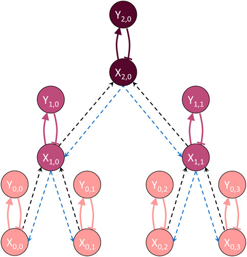
Figure 12. Hierarchical oscillator system with three scales. Each oscillator is an $(X,Y)$ pair and communication across scales by means of $X$ concentration values.

In this system, communication occurs across scales only (i.e., oscillators at a given scale do not communicate directly with each other). The abstracted information contained in oscillator $i$ at scale $S_m$ is the average $X$ concentration of its children oscillators in $S_{m-1}$ and is given by ${\bar{X}}_{m,i}(\cdot )$. The control information received by oscillator $i$ in $S_m$ is the $X$ concentration of its parent oscillator in $S_{m+1}$, which impacts the $X$ concentration of oscillator $i$ through Equation 45. The function ${\mathrm{\Gamma }}_{m,i}(t-{\tau }_m)$ in Equation 47 shows how both the abstracted and reified information impact the behavior of oscillator $i$ in $S_m$, with $W$ controlling the relative importance of both types of information. For the top and bottom scales, $\mathrm{\Gamma }$ is modified to eliminate the first and second terms, respectively, due to a lack of reified information from above and lack of aggregated information from below. Communication between oscillators happens through multiple feedback loops in which the $X$ concentration is collected from the immediate lower scale as averages, combined with the average from the immediate higher scale and sent back down as $X$ concentration with an associated time delay ${\tau }_m$. As in the case of a single pair of coupled oscillators, the behavior of the hierarchical system can achieve three steady-state conditions: synchronized oscillation, unsynchronized oscillation, and no oscillation. The overall goal is for the system to synchronize oscillators at the bottom scale.

4.5.2 Comparison strategies

To illustrate the information measures, we focus on two HO systems, both of which use NN type coupling but have two different scales (two- and three-scale). Both systems have four oscillators at the bottom scale $S_0$. The two-scale system has one oscillator at $S_1$ which receives the average of the four oscillators in $S_0$. The three-scale system (Figure 12) contains two oscillators in $S_1$ and one in $S_2$, and each oscillator receives the average $X$ concentration of its two children. Thus, the three-scale system breaks down the averaging into two steps, resulting in more delay in its structure since each oscillator at $S_1$ and $S_2$ passes down reified information with delay ${\tau }_m$.

The system is simulated using a time-delay ordinary differential equations (ODE) solver (details in Supplementary Material). The initial $X$ concentrations of the bottom scale oscillators are set to 0.2, 0.4, 0.6, and 0.8. The remaining oscillators are initialized to be the average values of their children. As a result, the results are deterministic, and one 300-s simulation is run for each system to allow for direct comparison between the two system structures. Parameters $F_m$ and ${\tau }_m$ were chosen so that the system achieved synchronized oscillation. Due to space constraints, the cases of unsynchronized or no oscillation are not considered.

To calculate $C_{\mathit{syn}}$, we assume that oscillators in $S_0$ have uniformly distributed $X$ concentrations on the interval [0,1], which represents the most random situation. The probability distributions at the higher scales are calculated using the Bates distribution. Integration for $Csyn$ is carried out numerically using the trapezoidal rule (for details, see Supplementary Material).

4.5.3 Information measures

4.5.3.1 Calculations

Since the HO system is modeled using differential equations which are continuous-time descriptions of the system behavior, the measures which use comparisons between $t$ and $t-\theta$ are calculated using derivatives in this case study.

4.5.3.1.1 Syntactic information

Due to the continuous nature of $X$ concentrations, syntactic information content cannot be calculated as in the other case studies using Shannon entropy or memory usage. Instead, we use a common entropy measure for continuous valued random variables, Jensen–Shannon (JS) divergence, between probability distributions $f_1$ and $f_2$ as defined in Equation 48 (Lin, 1991; Nielsen, 2019):

$D_{JS}\left(f_1\Vert f_2\right)=\frac{1}{2}\left(D_{KL}\left(f_1\Vert \bar{f}\right)+D_{KL}\left(f_2\Vert \bar{f}\right)\right)(48)$

where $\bar{f}=\frac{f_1+f_2}{2}$ and $D_{KL}$ is the Kullback–Leibler (KL) divergence (Kullback and Leibler, 1951):

$D_{KL}\left(p\Vert q\right)={\int }_{x\in \chi }p\left(x\right)\log \frac{p\left(x\right)}{q\left(x\right)}dx,(49)$

where $\chi$ is the support of $X$.

The JS divergence provides a metric to measure the difference between probability distributions. $D_{JS}\in [0,\log (2)]$ with $D_{JS}=0$ indicates that the two distributions are identical, and higher values indicate they are more dissimilar. We use $D_{JS}(f_{m,i}\Vert U)$ to calculate the amount of information contained in oscillator $i$ at scale $S_m$ compared to uniform distribution $U$. That is, the syntactic information for any given oscillator is calculated as

$C_{sy{n}_{m,i}}=1-\frac{D_{JS}\left(f_{m,i}\Vert U\right)}{\log \left(2\right)}(50)$

Using this definition, $C_{sy{n}_{m,i}}\in [\mathrm{0,1}]$, with values of 0 and 1 indicating the minimum and maximum amount of information, respectively. Syntactic information content for the system $C_{\mathit{syn}}$ is calculated as the sum of $C_{sy{n}_{m,i}}$ over all oscillators at all scales in the hierarchy.

$C_{\mathit{syn}}={\displaystyle \sum _{m=0}^{M-1}}{\displaystyle \sum _{i=0}^{N_m-1}}{C}_{sy{n}_{m,i}}(51)$

4.5.3.1.2 Semantic information

This case study does not involve changes to the differential equation model itself, so the semantic delta measures how much change there is to the knowledge ${\mathrm{\Gamma }}_{m,i}$ being used by oscillator $i$ at scale $S_m$. For the lowest scale of oscillators, ${\mathrm{\Gamma }}_{0,i}=X_{1,p_{0,i}}$, the average $X$ concentration passed down to oscillator $i$ from its parent $p_{0,i}$ with a delay of ${\tau }_0$.

${\mathrm{\Delta }}_{sm}\left(t\right)=\frac{1}{N_0}{\displaystyle \sum _{i=0}^{N_0-1}}\frac{d{X}_{1,p_{0,i}}\left(t-{\tau }_0\right)}{dt}(52)$

The ground truth $X_{th}$ for the system is the average $X$ concentration among all oscillators at the lowest scale, which is calculated as

$X_{th}\left(t\right)=\frac{1}{N_0}{\displaystyle \sum _{i=0}^{N_0-1}}{X}_{0,i}\left(t\right)(53)$

The semantic truth value is then calculated as

$V_{sm,th}\left(t\right)=-\frac{1}{N_0}{\displaystyle \sum _{i=0}^{N_0-1}}\frac{d}{dt}\left|X_{th}\left(t\right)-X_{1,p_{0,i}}\left(t-{\tau }_0\right)\right|(54)$

The efficiency is calculated by dividing the semantic truth value by $C_{\mathit{syn}}$.

$E_{sm,th}\left(t\right)=\frac{V_{sm,th}\left(t\right)}{C_{\mathit{syn,tot}}}(55)$

4.5.3.1.3 Pragmatic information

An action taken by an oscillator is to change its $X$ concentration based on the micro- and/or macro-information it receives about $X$ concentrations in the overall system, with the scope of this information determined by its location in the hierarchy. Thus, the numerical value of the action is calculated using Equation 45, and the pragmatic delta ${\mathrm{\Delta }}_{pr}$ is calculated as

${\mathrm{\Delta }}_{pr}\left(t\right)=\frac{1}{N_0}{\displaystyle \sum _{i=0}^{N_0-1}}\frac{d}{dt}\left(\frac{d{X}_{0,i}}{dt}\right)(56)$

Since the goal is to achieve synchronized oscillation at the lowest scale, the result is identical concentrations of $X$ among these oscillators at every moment $t$. The distance from this goal, or delta of goal ${\mathrm{\Delta }}_{gl}(t)$, is the variance of $X$, and its negative derivative is the pragmatic goal value $V_{pr,gl}(t)$.

${\mathrm{\Delta }}_{gl}\left(t\right)=\frac{1}{N_0}{\displaystyle \sum _{i=0}^{N_0-1}}{\left(X_{0,i}\left(t\right)-\mu \left(t\right)\right)}^2(57)$

where $\mu (t)=\frac{1}{N_0}{\sum }_{i=0}^{N_0-1}{X}_{0,i}(t)$

$V_{pr,gl}\left(t\right)=\frac{d{\mathrm{\Delta }}_{gl}\left(t\right)}{dt}(58)$

The efficiency is calculated by dividing the pragmatic goal value by $C_{\mathit{syn}}$.

$E_{pr,gl}\left(t\right)=\frac{V_{pr,gl}\left(t\right)}{C_{\mathit{syn}}}(59)$

4.5.3.2 Results

Figure 13 shows $C_{\mathit{syn}}$ results for the two HO systems under study. The three plots in the middle represent the probability density functions at each scale. For the three-scale system, the oscillators at the middle scale receive the average of the two children oscillators below it, resulting in a triangle distribution as shown in the middle plot. The highest scale oscillator receives the average of the two oscillators below it with triangle distributions, which is equivalent to the average of the four uniform distributions at the bottom scale. The values for $C_{sy{n}_{m,i}}$ are shown for each of the three scales. $C_{\mathit{syn}}$ is obtained by summing the values. Thus, for the three-scale system, $C_{\mathit{syn}}=(4\times 1)+(2\times 0.9271)+0.7917=6.6459$, while for the two-scale system $C_{\mathit{syn}}=(4\times 1)+0.7917=4.7917$. These values indicate that more information is contained in the three- than the two-scale system, making the latter a more efficient structure for achieving the same result.

Figure 13

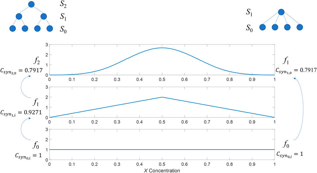
Figure 13. Calculated values for syntactic information. Left side of the figure depicts the three-scale system, right side depicts two-scale system.

Figure 14a shows the $X$ concentrations for the four bottom scale oscillators for each system. It is clear that the two-scale system synchronizes much faster than the three-scale system.

Figure 14

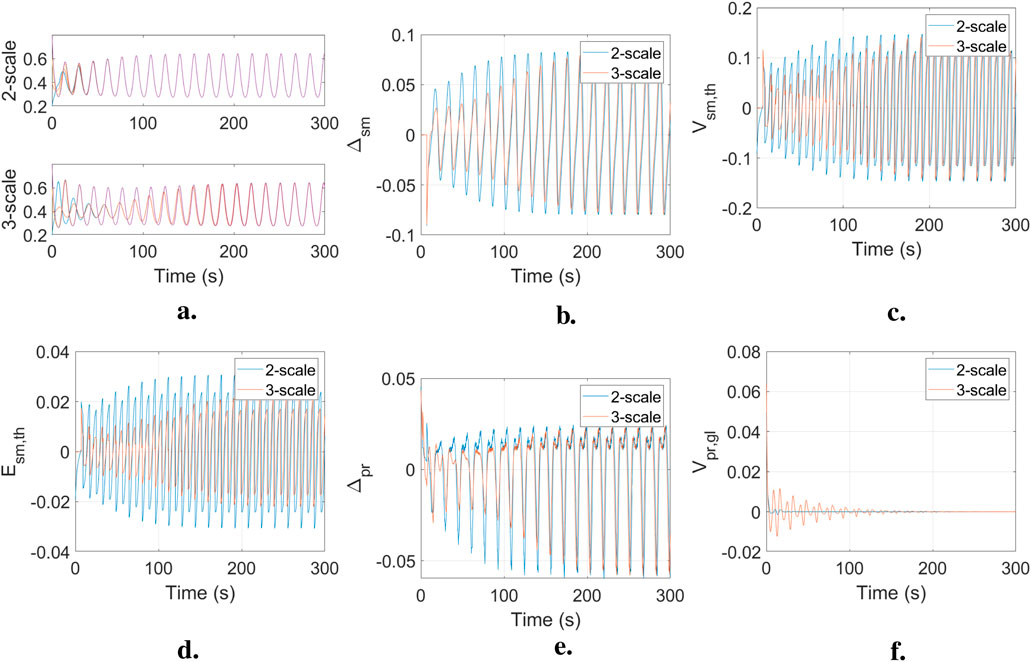
Figure 14. Results for the two hierarchical oscillator systems. Blue line shows the two-scale system and red line shows the three-scale system. (a) $X$ concentrations; (b) semantic delta; (c) semantic truth value; (d) semantic truth value efficiency; (e) pragmatic delta; (f) pragmatic goal value.

Figures 14b–f show the information measures for the two HO system plotted together for comparison. As information is passed through the system in the form of $X$ concentrations, which are oscillatory in nature, most information measures themselves oscillate. When viewed together, such information measures for each system have a small time offset due to oscillators in the two-scale system being slightly out of phase with those in the three-scale system. In all the information measures, there is a distinct change in behavior when the systems transition from unsynchronized to synchronized oscillations. During synchronization, all information measures (except efficiencies) are the same in both systems.

For the semantic delta, positive values indicate that the knowledge used by the oscillators to act is growing. Larger magnitudes indicate faster knowledge change. The three-scale system exhibits a smaller $|{\mathrm{\Delta }}_{sm}|$ than the two-scale system during the pre-synchronization period. This relationship indicates that the feedback in the two-scale system has a larger impact on the knowledge used by the oscillators to adapt their $X$ concentrations. Once synchronization is achieved, both systems have identical ${\mathrm{\Delta }}_{sm}(t)$, meaning that they achieve the same impact on an oscillator’s knowledge.

For the semantic truth value, positive values indicate that the average knowledge among the oscillators is getting closer to the ground truth. As with the ${\mathrm{\Delta }}_{sm}$, $|V_{sm,th}|$ is smaller for the three-scale system during the pre-synchronization period, leading to the conclusion that the two-scale system achieves more impact in bringing an oscillators’ knowledge closer to the ground truth. In addition, during synchronized operation, $V_{sm,th}$ for both is identical, but $E_{sm,th}$ emphasizes that the two-scale system achieves noticeably larger efficiency values (maximum of 0.03 vs 0.02 for the three-scale system) due to less information flowing in the system.

For the pragmatic delta, larger magnitudes indicate a larger change in the oscillator’s adaptation. The two-scale system achieves more change in adaptation during the pre-synchronization period, while the two systems have identical ${\mathrm{\Delta }}_{pr}$ once synchronized. Since the distance from the goal is measured as the variance in the $X$ concentrations among oscillators, a positive $V_{pr,gl}$ indicates that the system is moving toward the goal of synchronization; larger positive magnitudes indicate that it is moving toward the goal at a faster rate. In comparing the two systems, the three-scale system moves faster toward the goal, but this is offset by faster movement away from the goal in nearly equal amounts due to greater time lags in each oscillator’s knowledge. Thus, the three-scale system shows a greater degree of overshoot and undershoot on its way toward the goal, while the two-scale system is more direct and faster in its approach toward synchronization. As with $E_{sm,th}$, $E_{pr,gl}$ indicates that the two-scale system is more efficient in achieving synchronization.

5 Discussion and conclusion

CAS typically consist of many components that interact with each other across at least two scales (Ahl and Allen, 1996; Salthe, 1993), adapting through feedback loops to reach a shared goal (Flack et al., 2013). In such MSFS, there is always a loss of syntactic information when abstracting from the micro to the macro scale. Conversely, control information flowing from the macro to the micro can be either further abstracted (e.g., different macro-states may issue the same micro-controls), stay the same (e.g., through top-down forwarding), or gain information (e.g., through extra micro-scale context). Syntactic information measures, including Shannon entropy, can be used to quantify the size of these information flows and the amount of information abstracted across scales (as shown in the hierarchical oscillator and task distribution case studies). As information becomes more symbolic, the relevance of syntactic measures decreases, calling for value-oriented measures.

We propose a non-exhaustive set of information measures within the syntactic, semantic, and pragmatic categories, exemplified their usage through four cases of MSFS, although the measures could be applied more generally to all types of CAS, including single-scale CAS. Feedback is central to the behavior of all adaptive information-processing systems. Whenever there is a feedback cycle, there is a system that adapts and an information flow controlling that system. The inherent delays and uncertainties of the adapting system and its environment play a key part in the efficacy and efficiency of the feedback cycle. When the feedback spans multiple scales, affecting components that function at different granularities of time and information, it becomes increasingly divicult to adjust its operation to the multitude of delays and uncertainties. The presence of multiple feedback cycles that operate simultaneously between different scales exacerbates this difficulty. To deal with such increased complexity, parts of the system become quasi-independent (Simon, 2012), with minimal information flows coordinating them to reach a shared goal. Tracking information flows and their mutual influences throughout such MSFS becomes essential for understanding their behavior and/or adjusting their design. Using different types of information measures, which can be calculated for the whole system or at single scales, can help us understand such increased complexity in MSFS. This requires identifying a goal. Goals can be determined at different scales and can be exogenous or endogenous, depending on where the observer is placed. Observer identification is necessary for all types of information measures, including syntactic, while the goal choice is needed to measure informational values (semantic and pragmatic).

Such information measures are interrelated and best understood when considered simultaneously. Disturbances on the information flow (measured syntactically) have an impact on knowledge (measured semantically) and adaptation (measured pragmatically). In our examples, these disturbances were due to time delays or partial (and/or imperfect) information collection. Time delays can occur in information communication and processing or in system adaptation. Within feedback cycles, they can be tracked by comparing changes in actual state measures and in their semantic and pragmatic values over time at different scales. Depending on the system characteristics, delays can be beneficial in achieving the goal. This is so when the delay in the feedback cycle matches a slow and inaccurate adaptation process. In the robotic collective, for example, adaptation delays caused by the robots’ spatial dynamics compensated for inaccuracies in their collective state information that influence their movement. In the collective decision-making case, inaccurate information (i.e., an inaccurate collective opinion $O_{\mathit{coll}}$) leading to fast decisions performed better than accurate information that caused a longer feedback cycle. In the task distribution example, delays caused outdated state information for which adaptation strategies had to compensate. In Mellodge et al. (2021), we showed how delays could lead to adaptation towards different attractors, or goals. This includes the hierarchical oscillator example, where delays are essential to system synchronization. Our initial considerations on the potential benefits of delays in MSFS are limited to the cases that we considered, and it would be interesting to study different types of systems in order to generalize these conclusions and reach a better understanding of the role played by timing dynamics in CAS.

Partial or imperfect information leads to inaccurate collective knowledge. Studying the delta of truth ${\mathrm{\Delta }}_{th}$ together with the semantic delta value $V_{sm,th}$ over time can show whether the system accumulates inaccuracies as it acquires knowledge, learns to diminish them, or maintains them within a constant range (this latter case applying to all examples shown here). Trade-offs in knowledge acquisition can also be introduced by the abstraction process. In the robotics case, although the macro-scale information is derived by abstracting meso-scale information, comparing measures across scales did not result in the same performance ranking across different strategies, showing how a strategy that improves knowledge precision at one scale may reduce precision at a higher scale. Knowledge inaccuracies propagate through multi-scale systems, impacting adaptation towards the goal. This is observed by considering the semantic truth value $V_{sm,th}$ together with the pragmatic goal value $V_{pr,gl}$. In the task distribution case, perfect knowledge (as implemented by the model strategy) led to maximum efficacy in reaching the goal, even if the knowledge is outdated. In comparison, the BB strategy achieved the same $V_{pr,gl}$ with a lower accuracy of knowledge on the management scales but over a longer period. In the short term, the random strategy (RS) used no collective knowledge and performed similarly to BB. These insights can help tune the system configuration and strategy depending on the targeted timescale and goal—for example, RS may be efficient in highly fluctuating or unpredictable environments. The robotic collective example showed a different relation between semantic and pragmatic measures. Accurate knowledge hindered efficacy due to adaptive overreactions and execution delays. The ground truth strategy gave robots perfect knowledge of their collective state, but their individual reactions led to large oscillations around the goal state compared to the partial knowledge scenario.

In the collective decision-making model, semantic and pragmatic measures tracked the impact of varying system parameters (the number of agents $N$ and of information sources $R$) on collective knowledge and adaptation. The $rando{m}_{CN}$ strategy led to a higher pragmatic goal value $V_{pr,gl}$ for low $R$ than the $consensus$ strategy, despite having a higher average delta of truth ${\mathrm{\Delta }}_{th}$, showing how this performance is a result of a fast feedback cycle rather than accurate knowledge. This leads to fast and tight oscillations and variations of $O_{\mathit{coll}}$, which could be beneficial or not depending on the chosen system goal. Tuning the $consensus$ strategy to environmental conditions, on the other hand, can lead to smoother parameter transitions, enhancing resilience and scalability. In the hierarchical oscillator model, oscillating semantic measures lead to oscillating pragmatic measures, both in the two- and three-scale designs. This highlights the underlying oscillations of adaptations, which are essential to maintaining the biochemical oscillators while synchronizing them. Since perfect information does not always lead to the best adaptation, the semantic goal value (not calculated in the examples) could be used to find the most effective and efficient information flows for a given system. Still, tailoring information flows to a specific configuration may hinder transferability, so the semantic truth value and semantic goal value are best considered simultaneously—assuming that the ground truth can provide a common denominator across configuration and parameter ranges.

These examples provide initial insights into how coupled information measures can be used to understand the behavior of CAS. Specific calculations and measure sub-types are dependent on the chosen case study and application domain; expanding these will help further generalize the definition of information measures and their calculations. Here, including case studies featuring experimental data would be particularly valuable. This can help system analysts and designers study the value of information flows for system properties, such as reactivity, stability, and scalability. When paired with reinforcement learning methods, such insights can help improve systems’ real-time adaptation. Large language models (LLMs), for example, may learn to correlate the information measures with adaptation performance indicators, enabling the system to adapt its control processes, which is in line with recent approaches to implementing LLMs within multi-agent systems (Bo et al., 2024; De Curtò and De Zarzà, 2025). The proposed semantic information measures could also be employed to assess the impact of collected information on a system’s LLM in terms of actual changes and consequent performance. Beyond system analysis and performance, identifying how different patterns of information flows correlate with the behavior and evolution of CAS across scales can help characterize existing CAS through a unified informational lens (Krakauer et al., 2020) and understand fundamental regularities across such systems, contributing to a deeper theoretical understanding of the informational nature of CAS.

Data availability statement

The raw data supporting the conclusions of this article will be made available by the authors without undue reservation.

Author contributions

LJDF: Methodology, Writing – review and editing, Writing – original draft, Investigation, Conceptualization, Formal Analysis, Visualization, Data curation, Project administration. AD: Data curation, Visualization, Methodology, Conceptualization, Investigation, Writing – review and editing, Formal Analysis, Writing – original draft. PZ: Writing – review and editing, Data curation, Writing – original draft, Conceptualization, Investigation, Methodology, Visualization, Formal Analysis. PM: Conceptualization, Data curation, Writing – review and editing, Methodology, Writing – original draft, Formal Analysis, Investigation, Visualization.

Funding

The author(s) declare that financial support was received for the research and/or publication of this article. LJDF acknowledges funding by the Margarita Salas program of the Spanish Ministry of Universities, funded by the European Union-NextGeneraionEU.

Conflict of interest

The authors declare that the research was conducted in the absence of any commercial or financial relationships that could be construed as a potential conflict of interest.

Generative AI statement

The author(s) declare that no Generative AI was used in the creation of this manuscript.

Publisher’s note

All claims expressed in this article are solely those of the authors and do not necessarily represent those of their affiliated organizations, or those of the publisher, the editors and the reviewers. Any product that may be evaluated in this article, or claim that may be made by its manufacturer, is not guaranteed or endorsed by the publisher.

Supplementary material

The Supplementary Material for this article can be found online at: https://www.frontiersin.org/articles/10.3389/fcpxs.2025.1612142/full#supplementary-material

References

Ahl, V., and Allen, T. F. (1996). Hierarchy theory: a vision, vocabulary, and epistemology. Columbia University Press.

Google Scholar

Atmanspacher, H. (1991). Information dynamics. Plenum Press.

Google Scholar

Bellman, K. L., and Goldberg, L. J. (1984). Common origin of linguistic and movement abilities. Am. J. Physiology-Regulatory, Integr. Comp. Physiology 246, R915–R921. doi:10.1152/ajpregu.1984.246.6.R915

PubMed Abstract | CrossRef Full Text | Google Scholar

Bellman, K. L., Diaconescu, A., and Tomforde, S. (2021). Special issue on self-improving self integration. Future Gener. Comput. Syst. 119, 136–139. doi:10.1016/J.FUTURE.2021.02.010

CrossRef Full Text | Google Scholar

Bo, X., Zhang, Z., Dai, Q., Feng, X., Wang, L., Li, R., et al. (2024). Reflective multi-agent collaboration based on large language models. Adv. Neural Inf. Process. Syst. 37, 138595–138631.

Google Scholar

Brillouin, L. (1953). The negentropy principle of information. J. Appl. Phys. 24, 1152–1163. doi:10.1063/1.1721463

CrossRef Full Text | Google Scholar

Brillouin, L., and Gottschalk, C. M. (1962). Science and information theory. Phys. Today 15, 68. doi:10.1063/1.3057866

CrossRef Full Text | Google Scholar

De Curtò, J., and De Zarzà, I. (2025). Llm-driven social influence for cooperative behavior in multi-agent systems. IEEE Access. 44330–44342. doi:10.1109/ACCESS.2025.3548451

CrossRef Full Text | Google Scholar

Dessalles, J.-L. (2010). “Emotion in good luck and bad luck: predictions from simplicity theory,” in Proceedings of the 32nd annual conference of the cognitive science society. Editors S. Ohlsson, and R. Catrambone (Austin, TX: Cognitive Science Society), 1928–1933.

Google Scholar

Dessalles, J.-L. (2013). “Algorithmic simplicity and relevance,” in Algorithmic probability and friends - lnai 7070. Editor D. L. Dowe (Berlin: Springer Verlag), 119–130. doi:10.1007/978-3-642-44958-1_9

CrossRef Full Text | Google Scholar

Diaconescu, A., Di Felice, L. J., and Mellodge, P. (2019). “Multi-scale feedbacks for large-scale coordination in self-systems,” in 2019 IEEE 13th international conference on self-adaptive and self-organizing systems (SASO) (IEEE), 137–142.

CrossRef Full Text | Google Scholar

Diaconescu, A., Di Felice, L. J., and Mellodge, P. (2021a). Exogenous coordination in multi-scale systems: how information flows and timing affect system properties. Future Gener. Comput. Syst. 114, 403–426. doi:10.1016/j.future.2020.07.034

CrossRef Full Text | Google Scholar

Diaconescu, A., Di Felice, L. J., and Mellodge, P. (2021b). “An information-oriented view of multi-scale systems,” in 2021 IEEE international conference on autonomic computing and self-organizing systems companion (ACSOS-C) (IEEE), 154–159.

CrossRef Full Text | Google Scholar

Di Felice, L. J., and Zahadat, P. (2022). “An agent-based model of collective decision-making in correlated environments,” in Proceedings of the 4th International Workshop on Agent-Based Modelling of Human Behaviour (ABMHuB’22).

Google Scholar

Feistel, R., and Ebeling, W. (2016). Entropy and the self-organization of information and value. Entropy 18, 193. doi:10.3390/e18050193

CrossRef Full Text | Google Scholar

Fetzer, J. H. (2004). Information: does it have to be true? Minds Mach. 14, 223–229. doi:10.1023/b:mind.0000021682.61365.56

CrossRef Full Text | Google Scholar

Flack, J. (2021). “Complexity begets complexity,”Conf. Artif. 7. doi:10.1162/isal_a_00470

CrossRef Full Text | Google Scholar

Flack, J. C. (2017). Coarse-graining as a downward causation mechanism. Philosophical Trans. R. Soc. A Math. Phys. Eng. Sci. 375, 20160338. doi:10.1098/rsta.2016.0338

PubMed Abstract | CrossRef Full Text | Google Scholar

Flack, J. C., Erwin, D., Elliot, T., and Krakauer, D. C. (2013). Timescales, symmetry, and uncertainty reduction in the origins of hierarchy in biological systems. In Evolution cooperation and complexity (Editors K Sterelny, R Joyce, B Calcott, and B Fraser), 45–74. Cambridge, MA: MIT Press.

Google Scholar

Floridi, L. (2005). Is semantic information meaningful data? Philosophy phenomenological Res. 70, 351–370. doi:10.1111/j.1933-1592.2005.tb00531.x

CrossRef Full Text | Google Scholar

Floridi, L. (2008). A defence of informational structural realism. Synthese 161, 219–253. doi:10.1007/s11229-007-9163-z

CrossRef Full Text | Google Scholar

Frank, A. U. (2003). Pragmatic information content—how to measure the information in a route. Found. Geogr. Inf. Sci. 47.

Google Scholar

Gernert, D. (2006). Pragmatic information: historical exposition and general overview. Mind Matter 4(2):, 141–167.

Google Scholar

Gould, J. P. (1974). Risk, stochastic preference, and the value of information. J. Econ. Theory 8, 64–84. doi:10.1016/0022-0531(74)90006-4

CrossRef Full Text | Google Scholar

Grunwald, P. D., and Vitanyi, P. M. (2008). “Algorithmic information theory,” in Philosophy of information (Elsevier).

Google Scholar

Haken, H., and Portugali, J. (2016). Information and self-organization. Entropy 19, 18. doi:10.3390/e19010018

CrossRef Full Text | Google Scholar

Jablonka, E. (2002). Information: its interpretation, its inheritance, and its sharing. Philosophy Sci. 69, 578–605. doi:10.1086/344621

CrossRef Full Text | Google Scholar

Kephart, J., and Chess, D. (2003). The vision of autonomic computing. Computer 36, 41–50. doi:10.1109/MC.2003.1160055

CrossRef Full Text | Google Scholar

Kim, J.-R., Shin, D., Jung, S. H., Heslop-Harrison, P., and Cho, K.-H. (2010). A design principle underlying the synchronization of oscillations in cellular systems. J. Cell Sci. 123, 537–543. doi:10.1242/jcs.060061

PubMed Abstract | CrossRef Full Text | Google Scholar

Kolchinsky, A., and Wolpert, D. H. (2018). Semantic information, autonomous agency and non-equilibrium statistical physics. Interface focus 8, 20180041. doi:10.1098/rsfs.2018.0041

PubMed Abstract | CrossRef Full Text | Google Scholar

Kounev, S., Lewis, P. R., Bellman, K. L., Bencomo, N., Cámara, J., Diaconescu, A., et al. (2017). “The notion of self-aware computing,” in Self-aware computing systems. Editors S. Kounev, J. O. Kephart, A. Milenkoski, and X. Zhu (Springer International Publishing), 3–16. doi:10.1007/978-3-319-47474-8_1

CrossRef Full Text | Google Scholar

Krakauer, D., Bertschinger, N., Olbrich, E., Flack, J. C., and Ay, N. (2020). The information theory of individuality. Theory Biosci. 139, 209–223. doi:10.1007/s12064-020-00313-7

PubMed Abstract | CrossRef Full Text | Google Scholar

Kullback, S., and Leibler, R. A. (1951). On information and sufficiency. Ann. Math. statistics 22, 79–86. doi:10.1214/aoms/1177729694

CrossRef Full Text | Google Scholar

Lalanda, P., McCann, J., and Diaconescu, A. (2013a). “Autonomic computing: principles, design and implementation,” in Undergraduate topics in computer science. Springer London.

Google Scholar

Lalanda, P., McCann, J. A., and Diaconescu, A. (2013b). “Autonomic computing - principles, design and implementation,” in Undergraduate topics in computer science. Springer. doi:10.1007/978-1-4471-5007-7

CrossRef Full Text | Google Scholar

Lewis, G. N. (1930). The symmetry of time in physics. Science 71, 569–577. doi:10.1126/science.71.1849.569

PubMed Abstract | CrossRef Full Text | Google Scholar

Lin, J. (1991). Divergence measures based on the shannon entropy. IEEE Trans. Inf. Theory 37, 145–151. doi:10.1109/18.61115

CrossRef Full Text | Google Scholar

Mellodge, P., Diaconescu, A., and Di Felice, L. J. (2021). “Timing configurations affect the macro-properties of multi-scale feedback systems,” in 2021 IEEE international conference on autonomic computing and self-organizing systems (ACSOS) (Los Alamitos, CA, USA: IEEE Computer Society), 100–109. doi:10.1109/ACSOS52086.2021.00032

CrossRef Full Text | Google Scholar

Ming Li, P. V. (2019). “An introduction to Kolmogorov complexity and its applications,” in Texts in computer science. Springer Cham. doi:10.1007/978-3-030-11298-1

CrossRef Full Text | Google Scholar

Morris, C. (1938). Foundations of the theory of signs. In International encyclopedia of unified science. Chicago: Chicago University Press. 1–59.

Google Scholar

Müller-Schloer, C., Schmeck, H., and Ungerer, T. (2011). “Organic computing — a paradigm shift for complex systems,” in Autonomic systems. Springer Basel.

Google Scholar

Müller-Schloer, C., and Tomforde, S. (2017). “Organic computing – technical systems for survival in the real world,” in Autonomic systems.

Google Scholar

Nehaniv, C. L. (1999). “Meaning for observers and agents,” in Proceedings of the 1999 IEEE international symposium on intelligent control intelligent systems and semiotics (cat. No. 99CH37014) (IEEE), 435–440.

CrossRef Full Text | Google Scholar

Nielsen, F. (2019). On the jensen–shannon symmetrization of distances relying on abstract means. Entropy 21, 485. doi:10.3390/e21050485

PubMed Abstract | CrossRef Full Text | Google Scholar

Pattee, H. H. (1973). Hierarchy theory; the challenge of complex systems. New York: G. Braziller.

Google Scholar

Roederer, J. G., et al. (2005). Information and its role in nature. Springer.

Google Scholar

Salthe, S. N. (1993). Development and evolution: complexity and change in biology. Cambridge, MA: Mit Press.

Google Scholar

Shannon, C. E. (1948). A mathematical theory of communication. Bell Syst. Tech. J. 27, 379–423. doi:10.1002/j.1538-7305.1948.tb01338.x

CrossRef Full Text | Google Scholar

Simon, H. A. (1991). The architecture of complexity. Boston, MA: Springer US. doi:10.1007/978-1-4899-0718-9_31

CrossRef Full Text | Google Scholar

Simon, H. A. (2012). “The architecture of complexity,” in The roots of logistics (Springer), 335–361.

Google Scholar

Sowinski, D. R., Carroll-Nellenback, J., Markwick, R. N., Piñero, J., Gleiser, M., Kolchinsky, A., et al. (2023). Semantic information in a model of resource gathering agents. PRX Life 1, 023003. arXiv preprint arXiv:2304.03286. doi:10.1103/prxlife.1.023003

CrossRef Full Text | Google Scholar

Theraulaz, G., Bonabeau, E., and Deneubourg, J.-L. (1998). Response threshold reinforcement and division of labour in insect societies, Proceedings of the Royal Society B: Biological Sciences, 265(1393):327–332.

Google Scholar

Timpson, C. G. (2013). Quantum information theory and the foundations of quantum mechanics. Oxford: OUP.

Google Scholar

Tribus, M., and McIrvine, E. C. (1971). Energy and information. Sci. Am. 225, 179–188. doi:10.1038/scientificamerican0971-179

CrossRef Full Text | Google Scholar

Uexküll von, J. (2013). A Foray Into the Worlds of Animals and Humans: With a Theory of Meaning. Minneapolis, MN: University of Minnesota Press.

Google Scholar

Walker, S. I. (2014). Top-down causation and the rise of information in the emergence of life. Information 5, 424–439. doi:10.3390/info5030424

CrossRef Full Text | Google Scholar

Weinberger, E. D. (2002). A theory of pragmatic information and its application to the quasi-species model of biological evolution. Biosystems 66, 105–119. doi:10.1016/s0303-2647(02)00038-2

PubMed Abstract | CrossRef Full Text | Google Scholar

Weizsäcker, E. U. v., and Weizsäcker, C. v. (1972). Wiederaufnahme der begrifflichen frage: Was ist information. Nova Acta Leopoldina 37, 535–555.

Google Scholar

Weyns, D. (2021). “Basic principles of self-adaptation and conceptual model,”. John Wiley and Sons, Ltd, 1–15. doi:10.1002/9781119574910.ch1

CrossRef Full Text | Google Scholar

Wong, T., Wagner, M., and Treude, C. (2022). Self-adaptive systems: a systematic literature review across categories and domains. Inf. Softw. Technol. 148, 106934. doi:10.1016/j.infsof.2022.106934

CrossRef Full Text | Google Scholar

Zahadat, P. (2023). “Local estimation vs global information: the benefits of slower timescales,” in 4th IEEE International Conference on Autonomic Computing and Self-Organizing Systems (ACSOS). 29–30. doi:10.1109/acsos-c58168.2023.00030

CrossRef Full Text | Google Scholar