Cascade Descriptor Observers: Application to Understanding Sitting Control of Persons Living With Spinal Cord Injury

Introduction

People with spinal cord injury (SCI) live with a complete or a partial paralysis of their abdominal and lower back muscles. The consequences on sitting control are visible in everyday activities: either reaching, taking objects, or accessing transport. Among the rehabilitation protocols offered to people with SCI, exercises are designed to teach new motor patterns to stabilize the upper part of the trunk, only through movements of the head and upper limbs (Janssen-Potten et al., 1999). Actually, the occupational therapist has no means of objectively following the learning of these new motor patterns, which must nevertheless guarantee a certain stability of the person in a seated position. The authors aim to provide objective data for the occupational therapist, which should enable him to better follow the learning of new motor patterns aimed at stabilizing the upper part of the body through upper limbs in particular. The authors aim also, like other movements such as walking, to provide real-time estimations to the occupational therapist, such as joint torques and their evolution over time. These variables are unmeasurable by nature, except invasive approaches, and this study proposes a way to estimate them using a model approach. This study is a proof-of-concept work to derive non-measurable (unknown) inputs variables from high-sized non-linear models and apply to people living with SCI. The challenge faced is how to derive non-linear observers for high-sized systems that preserve at most the initial non-linear model. The main problem is that simplifications, such as partial linearization, will deteriorate the quality of the estimation, especially for the non-measured inputs as they are the “farthest” from the outputs, thus cumulating the imprecisions.

The case study concerns sitting control of persons living with SCI. This study comes from the difficulties to obtain performance results due to complexity and/or limitations of the results obtained previously¹. First of all, let us recall an important remark: the people with SCI can only mobilize their upper limbs to stabilize the sitting; thus, the main input torque available for a human, the trunk torque, is not functional. Considering the fact that the person cannot activate the muscles below the (complete) lesion and, therefore, no motor torque can be produced at this level to stabilize the upper part of the human body (when needed), people with SCI must, therefore, adopt new strategies to maintain their stability while sitting (Blandeau, 2018). Therefore, understanding how stability is preserved is important but difficult: the torques cannot be measured, the model is highly non-linear, open-loop is unstable, and closed-loop (in the sense of sensorimotor SCI internal control) is very weakly stable. Thus, modeling will also imply building an internal control to stabilize, which is out of the scope of this study, and has been done in Guerra et al. (2018). It implies a very restricted area of stabilization as very tiny disturbances may destabilize the sitting person with SCI. For the observation part, when using a relatively basic mechanical model called H2AT (for Head-Two-Arms-Trunk), non-linear observers expressed as quasi-LPV models were easily derived. “Easily” is interpreted as LMI constraints problems with a reasonable complexity compatible with actual solvers (Blandeau et al., 2018). From this preliminary H2AT model, a more complex model called S3S (Seated-3-Segment) has been built. It is a planar triple-inverted pendulum represented in the sagittal plane (2D) by the trunk, upper arm, and forearm segments. The idea is to go from its actual 2D-S3S to a 3D-S3S form. Nevertheless, in its 2D actual form and taking a global model, the number of states and non-linearities lead to LMI constraints problems that are already close to the limits of actual solvers, that is, for the brute way-of-doing thousands of constraints and millions of variables (Guerra et al., 2020). Recalling the initial goal of keeping a model the closest possible to reality, using appropriate techniques it is possible to solve the 2D-S3S observation problem with a unique model, but the fact that the optimization problem is close to the limits of the solvers, it is impossible to follow this way-of-doing to get any solution for a 3D-S3S. In order to be able to get feasible performance solutions, this study proposes to decompose the mechanical model under descriptor forms in interconnected systems, from where descriptor non-linear observers of reduced sizes can be derived from local problems (Lendek et al., 2008) (Gripa et al., 2012). It results in cascaded observers design for descriptor mechanical systems. We notice that partitioning approach applied to a non-linear system as well as in the observer design improves the modularity and reduce complexity of the initial problem which implies a reduction in computational costs (Lendek et al., 2010). The goal is, thus, to apply the methodology on the 2D-S3S model from where results are already available as well as from real-time experiments. We will show that the methodology is perfectly tractable, with formal proof of convergences and results comparable to the global form of observation used in¹.

The article is organized as follows. After some notations, the second part recalls the 2D-S3S model and quasi-LPV models or so-called Takagi–Sugeno ones. It also gives a first solution to the estimation of the variables with a unique model is provided in continuous as a basis of comparison. The third part proposes a second solution based on decomposition in two interconnected cascaded local models. It includes a global result of convergence for cascaded descriptor models estimation. The fourth part applies this cascade observer way-of-doing to the 2D-S3S model and proposes a solution as a LMI constraints problem to solve. Fifth part proposes the simulation and real-time experiments compared with the global 2D-S3S observer and shows the relevance of the approach.

Notations and Useful Material: the following notations are adopted all along the study. For a given variable, its argument can be omitted and replaced with $(\cdot )$, for general purpose or when there is no ambiguity. With matrices $A_i$, $i\in \left\{1,\dots ,r\right\}$ of appropriate dimension, we define a polytopic description in the following form: $A_h={\displaystyle \sum _{i=1}^r{h}_i(\cdot )A_i}$, with the nonlinear functions $h_i(\cdot )\ge 0$ being continuous and satisfying the convex sum property ${\displaystyle \sum _{i=1}^r{h}_i(\cdot )}=1$. As usual $(\ast )$ stands for a transpose quantity $Q+(\ast )$ for $Q+Q^T$, and in a matrix $(\ast )$ represents the transpose of the entry in the symmetric position. At last, $I_n\in {ℝ}^{n\times n}$ stands for the identity matrix and $0_n\in {ℝ}^{n\times n}$ for the matrix of null entries.

Statement of the Problem

The 2D-S3S model has been presented in Guerra et al. (2020) and only its equations are recalled therein. The model Figure 1 is a variation of the 2D triple-inverted pendulum represented in the sagittal plane by the trunk, upper arm, and forearm segments (i.e., segments 0, 1, and 2, respectively) and interconnected by revolute joints at points T (trunk), S (shoulder), and E (elbow), whereas the point H stands for hands. For a segment $i\in \left\{\mathrm{0,1,2}\right\}$, ${\mathrm{\Gamma }}_i\left(t\right)$ stands for the torque input, $G_i$ stands for its center of mass (COM), $m_i$ for its mass, $l_i$ its length, $l_{G_i}$ the length from origin to the COM, and ${\text{I}}_{G_i}$ its moment of inertia. Regression rules are previously used to obtain these constants for a typical 80 kg male (Fang et al., 2017). The relative set points correspond to: $q_0={\theta }_0$, $q_1+\pi ={\theta }_1-{\theta }_0$, and $q_2={\theta }_2-{\theta }_1$. These points correspond to the rest position, and $0rad$ corresponding to the hands-up position.

FIGURE 1

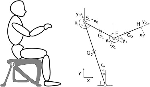
FIGURE 1. S3S Model, the joint T is free whereas joints S and E are active.

The system of dynamic equations of the S3S model is obtained by deriving the Lagrangian equation $L=E-U$ with $E={\displaystyle {\sum }_{i=0}^2{E}_i}$, the kinetic energy, and $U={\displaystyle {\sum }_{i=0}^2{U}_i}$, the potential energy, where the kinetic energy (respectively potential) of the system is equal to the sum of the energies of each solid. After some manipulations (see, Blandeau, 2018) the Lagrangian of the S3S model can be written as:

$\begin{array}{l}L=\frac{{\dot{\theta }}_0^2}{2}\left({\text{I}}_{G_0}+m_0{l}_{G_0}^2+m_1{l}_0^2+m_2{l}_0^2\right)+\frac{{\dot{\theta }}_1^2}{2}\left({\text{I}}_{G_1}+m_1{l}_{G_1}^2+m_2{l}_1^2\right)+\frac{{\dot{\theta }}_2^2}{2}\left({\text{I}}_{G_2}+m_2{l}_{G_2}^2\right)\\ -{\dot{\theta }}_0{\dot{\theta }}_1\left(m_1{l}_0{l}_{G_1}+m_2{l}_0{l}_1\right)\cos \left(q_1\right)+{\dot{\theta }}_0{\dot{\theta }}_2{m}_2{l}_0{l}_{G_2}\cos \left(q_2+q_1\right)+{\dot{\theta }}_1{\dot{\theta }}_2{m}_2{l}_1{l}_{G_2}\cos \left(q_2\right)\\ -m_{2}g{l}_{G_2}\cos \left({\theta }_2\right)-\left(m_{0}g{l}_{G_0}+m_{1}g{l}_0+m_{2}g{l}_0\right)\cos \left({\theta }_0\right)-\left(m_{1}g{l}_{G_1}+m_{2}g{l}_1\right)\cos \left({\theta }_1\right).\end{array}(1)$

For introducing simplicity in the expressions, $I_{q2}=I_{G_2}=m_2{l}_{G_2}^2,I_{q1}=I_{G_1}+I_{G_2}+m_2{l}_{G_2}^2+m_1{l}_{G_1}^2+m_2{l}_1^2$ and $I_{q0}=I_{G_0}+I_{G_1}+I_{G_2}+m_1{l}_{G_1}^2+m_2{l}_1^2+m_2{l}_{G_2}^2+m_0{l}_{G_0}^2+m_1{l}_0^2+m_2{l}_0^2$; the dynamic is described (Khalil and Dombre, 2004) using $\frac{d}{dt}\left(\frac{\partial L}{\partial {\dot{q}}_i}\right)-\frac{\partial L}{\partial q_i}={\mathrm{\Gamma }}_i$, $i\in \left\{\mathrm{0,1,2}\right\}$. It results in the following:

$\begin{array}{c}{\mathrm{\Gamma }}_0={\ddot{q}}_0\left(I_{q0}-2\left(m_1{l}_0{l}_{G_1}+m_2{l}_0{l}_1\right)\cos \left(q_1\right)-2m_2{l}_0{l}_{G_2}\cos \left(q_2+q_1\right)+2m_2{l}_1{l}_{G_2}\cos \left(q_2\right)\right)\\ +{\ddot{q}}_1\left(I_{q1}-\left(m_1{l}_0{l}_{G_1}+m_2{l}_0{l}_1\right)\cos \left(q_1\right)-m_2{l}_0{l}_{G_2}\cos \left(q_2+q_1\right)\right)\\ +{\ddot{q}}_2\left(I_{q2}-m_2{l}_0{l}_{G_2}\cos \left(q_2+q_1\right)+m_2{l}_1{l}_{G_2}\cos \left(q_2\right)\right)+{\dot{q}}_1^2\left(\left(m_1{l}_0{l}_{G_1}+m_2{l}_0{l}_1\right)\sin \left(q_1\right)+m_2{l}_0{l}_{G_2}\sin \left(q_2+q_1\right)\right)\\ +{\dot{q}}_2^2\left(m_2{l}_0{l}_{G_2}\sin \left(q_2+q_1\right)-m_2{l}_1{l}_{G_2}\sin \left(q_2\right)\right)+2{\dot{q}}_0{\dot{q}}_1\left(\left(m_1{l}_0{l}_{G_1}+m_2{l}_0{l}_1\right)\sin \left(q_1\right)+m_2{l}_0{l}_{G_2}\sin \left(q_2+q_1\right)\right)\\ +2{\dot{q}}_0{\dot{q}}_2\left(m_2{l}_0{l}_{G_2}\sin \left(q_2+q_1\right)-m_2{l}_1{l}_{G_2}\sin \left(q_2\right)\right)+2{\dot{q}}_1{\dot{q}}_2\left(m_2{l}_0{l}_{G_2}\sin \left(q_2+q_1\right)-m_2{l}_1{l}_{G_2}\sin \left(q_2\right)\right)\\ -\left(m_{0}g{l}_{G_0}+m_{1}g{l}_0+m_{2}g{l}_0\right)\sin \left(q_0\right)+\left(m_{1}g{l}_{G_1}+m_{2}g{l}_1\right)\sin \left(q_1+q_0\right)+m_{2}g{l}_{G_2}\sin \left(q_2+q_1+q_0\right),{\mathrm{\Gamma }}_1={\ddot{q}}_0\left(I_{q1}+2m_2{l}_1{l}_{G_2}\cos \left(q_2\right)-\left(m_1{l}_0{l}_{G_1}+m_2{l}_0{l}_1\right)\cos \left(q_1\right)-m_2{l}_0{l}_{G_2}\cos \left(q_2+q_1\right)\right)+{\ddot{q}}_1\left(I_{q1}+2m_2{l}_1{l}_{G_2}\cos \left(q_2\right)\right)\\ +{\ddot{q}}_2\left(I_{q2}+m_2{l}_1{l}_{G_2}\cos \left(q_2\right)\right)-{\dot{q}}_0^2\left(\left(m_1{l}_0{l}_{G_1}+m_2{l}_0{l}_1\right)\sin \left(q_1\right)+m_2{l}_0{l}_{G_2}\sin \left(q_2+q_1\right)\right)-{\dot{q}}_2^2{m}_2{l}_1{l}_{G_2}\sin \left(q_2\right)\\ -2{\dot{q}}_0{\dot{q}}_2{m}_2{l}_1{l}_{G_2}\sin \left(q_2\right)-2{\dot{q}}_1{\dot{q}}_2{m}_2{l}_1{l}_{G_2}\sin \left(q_2\right)+\left(m_{1}g{l}_{G_1}+m_{2}g{l}_1\right)\sin \left(q_1+q_0\right)+m_{2}g{l}_{G_2}\sin \left(q_2+q_1+q_0\right),\\ {\mathrm{\Gamma }}_2={\ddot{q}}_0\left(I_{q2}-m_2{l}_0{l}_{G_2}\cos \left(q_2+q_1\right)+m_2{l}_1{l}_{G_2}\cos \left(q_2\right)\right)+{\ddot{q}}_1\left(I_{q2}+m_2{l}_1{l}_{G_2}\cos \left(q_2\right)\right)+{\ddot{q}}_2{I}_{q2}\\ +{\dot{q}}_0^2\left(m_2{l}_1{l}_{G_2}\sin \left(q_2\right)-m_2{l}_0{l}_{G_2}\sin \left(q_2+q_1\right)\right)+{\dot{q}}_1^2{m}_2{l}_1{l}_{G_2}\sin \left(q_2\right)+2{\dot{q}}_0{\dot{q}}_1{m}_2{l}_1{l}_{G_2}\sin \left(q_2\right)+m_{2}g{l}_{G_2}\sin \left(q_2+q_1+q_0\right).\end{array}(2)$

With a state vector $x\left(t\right)=\left[\begin{array}{c}q\left(t\right)\\ \dot{q}\left(t\right)\end{array}\right]={\left[\begin{array}{cccccc}{q}_0& q_1& q_2& {\dot{q}}_0& {\dot{q}}_1& {\dot{q}}_2\end{array}\right]}^T\in {ℝ}^6$ the following non-linear system is obtained from Eq (2):

$\{\begin{array}{l}E\left(q\left(t\right)\right)\dot{x}\left(t\right)=A\left(x\left(t\right)\right)x\left(t\right)+S\left(q\left(t\right)\right)+Bu\left(t\right)\\ y\left(t\right)=Cx\left(t\right),\end{array}(3)$

where $y\left(t\right)=q\left(t\right)\in {ℝ}^3$ being the output vector, $u\left(t\right)={\left[\begin{array}{ccc}{\mathrm{\Gamma }}_0\left(t\right)& {\mathrm{\Gamma }}_1\left(t\right)& {\mathrm{\Gamma }}_2\left(t\right)\end{array}\right]}^T$ the torque inputs vector, $E\left(q\left(t\right)\right)=\left[\begin{array}{cc}{I}_3& 0_3\\ 0_3& \tilde{E}\left(q\left(t\right)\right)\end{array}\right]$, $A\left(x\left(t\right)\right)=\left[\begin{array}{cc}{0}_3& I_3\\ 0_3& \tilde{A}\left(x\left(t\right)\right)\end{array}\right]$, $S\left(q\left(t\right)\right)=\left[\begin{array}{c}{0}_{3\times 1}\\ \tilde{S}\left(q\left(t\right)\right)\end{array}\right]$, $B=\left[\begin{array}{c}{0}_{3\times 3}\\ I_3\end{array}\right]$, and $C=\left[\begin{array}{cc}{I}_3& 0_3\end{array}\right]$ and the following matrix expressions is obtained:

$\tilde{S}\left(q\right)=-\left[\begin{array}{ccc}-\left(m_{0}g{l}_{G_0}+m_{1}g{l}_0+m_{2}g{l}_0\right)& m_{1}g{l}_{G_1}+m_{2}g{l}_1& m_{2}g{l}_{G_2}\\ 0& m_{1}g{l}_{G_1}+m_{2}g{l}_1& m_{2}g{l}_{G_2}\\ 0& 0& m_{2}g{l}_{G_2}\end{array}\right]\left[\begin{array}{c}\sin \left(q_0\right)\\ \sin \left(q_1+q_0\right)\\ \sin \left(q_2+q_1+q_0\right)\end{array}\right],(4)$

$\begin{array}{l}\tilde{E}\left(q\right)={\left[e_{ij}\right]}_{i,j\in \left\{\mathrm{1,2,3}\right\}},\tilde{A}\left(x\right)={\left[a_{ij}\right]}_{i,j\in \left\{\mathrm{1,2,3}\right\}},e_{11}=I_{q0}-2\left(m_1{l}_0{l}_{G_1}+m_2{l}_0{l}_1\right)\cos \left(q_1\right)-2m_2{l}_0{l}_{G_2}\cos \left(q_2+q_1\right)\\ +2m_2{l}_1{l}_{G_2}\cos \left(q_2\right),e_{12}=I_{q1}+2m_2{l}_1{l}_{G_2}\cos \left(q_2\right)\\ -\left(m_1{l}_0{l}_{G_1}+m_2{l}_0{l}_1\right)\cos \left(q_1\right)-m_2{l}_0{l}_{G_2}\cos \left(q_2+q_1\right),e_{13}=I_{q2}-m_2{l}_0{l}_{G_2}\cos \left(q_2+q_1\right)+m_2{l}_1{l}_{G_2}\cos \left(q_2\right),e_{21}=I_{q1}-\left(m_1{l}_0{l}_{G_1}+m_2{l}_0{l}_1\right)\cos \left(q_1\right)-m_2{l}_0{l}_{G_2}\cos \left(q_2+q_1\right)\\ +2m_2{l}_1{l}_{G_2}\cos \left(q_2\right),e_{22}=I_{q1}+2m_2{l}_1{l}_{G_2}\cos \left(q_2\right),\end{array}(5)$

$e_{23}=I_{q2}+m_2{l}_1{l}_{G_2}\cos \left(q_2\right),e_{31}=I_{q2}-m_2{l}_0{l}_{G_2}\cos \left(q_2+q_1\right)+m_2{l}_1{l}_{G_2}\cos \left(q_2\right),$

$e_{32}=I_{q2}+m_2{l}_1{l}_{G_2}\cos \left(q_2\right),\mathrm{a}\mathrm{n}\mathrm{d}{e}_{33}=I_{q2}.$

$a_{11}={\dot{q}}_2{m}_2{l}_{G_2}\left(l_1\sin \left(q_2\right)-l_0\sin \left(q_2+q_1\right)\right)-{\dot{q}}_1\left(\left(m_1{l}_0{l}_{G_1}+m_2{l}_0{l}_1\right)\sin \left(q_1\right)+m_2{l}_0{l}_{G_2}\sin \left(q_2+q_1\right)\right),$

$a_{12}={\dot{q}}_2{m}_2{l}_{G_2}\left(l_1\sin \left(q_2\right)-l_0\sin \left(q_2+q_1\right)\right)-\left({\dot{q}}_1+{\dot{q}}_0\right)\left(\left(m_1{l}_0{l}_{G_1}+m_2{l}_0{l}_1\right)\sin \left(q_1\right)+m_2{l}_0{l}_{G_2}\sin \left(q_2+q_1\right)\right),$

$a_{13}=\left({\dot{q}}_0+{\dot{q}}_1+{\dot{q}}_2\right)m_2{l}_{G_2}\left(l_1\sin \left(q_2\right)-l_0\sin \left(q_2+q_1\right)\right),$

$a_{21}={\dot{q}}_0\left(\left(m_1{l}_0{l}_{G_1}+m_2{l}_0{l}_1\right)\sin \left(q_1\right)+m_2{l}_0{l}_{G_2}\sin \left(q_2+q_1\right)\right)+{\dot{q}}_2{m}_2{l}_1{l}_{G_2}\sin \left(q_2\right),$

$a_{22}={\dot{q}}_2{m}_2{l}_1{l}_{G_2}\sin \left(q_2\right),a_{23}=\left({\dot{q}}_0+{\dot{q}}_1+{\dot{q}}_2\right)m_2{l}_1{l}_{G_2}\sin \left(q_2\right),$

$a_{31}={\dot{q}}_0\left(m_2{l}_0{l}_{G_2}\sin \left(q_2+q_1\right)+m_2{l}_1{l}_{G_2}\sin \left(q_2\right)\right)-{\dot{q}}_1{m}_2{l}_1{l}_{G_2}\sin \left(q_2\right),$

$a_{32}=-\left({\dot{q}}_0+{\dot{q}}_1\right)m_2{l}_1{l}_{G_2}\sin \left(q_2\right),\mathrm{a}\mathrm{n}\mathrm{d}{a}_{33}=0.$

Remark 1: The descriptor form is common for mechanical systems; specifically, because it is a natural way to write equations derived from the Euler–Lagrange method (Skelton et al., 1997; Lendek, et al., 2018). For mechanical systems, the matrix $E\left[q\left(t\right)\right]$ generally ends up regular, as for the S3S model Eq. 3. Therefore, discussions about the singular case, observability and impulse-free modes (Varga, 1995) are not necessary. The way the problem of observation will be solved is using quasi-LPV or so-called T-S models (Tanaka and Wang 2001), and the Lyapunov approach and the solutions are obtained using sets of linear matrix inequalities (LMI) (Boyd et al., 1994). Notice that, as $E\left[q\left(t\right)\right]$ is regular, a classical state space representation can also be straightforwardly derived from Eq. 3. Nevertheless, a key point to reduce complexity (in term of LMI conservatism) is to keep a constant $B$ matrix (Bouarar, et al., 2010). Lastly, using a descriptor formulation such as Eq. 3 has been shown to lower the conservatism of the result by reducing the number of vertices (Lendek, et al., 2018) (Chadli and Darouach, 2012).

Designing an observer in the continuous case for systems such as model Eq. 3 is difficult for two reasons. The first one concerns the fact that the matrix $A\left[x\left(t\right)\right]$ depends on non-measured variables of $x\left(t\right)$. When dealing with a polytopic representation such as T-S models, it resumes in the so-called non-measured premise variables, which is still an open problem in the general case. The second reason is due to the size of the model and the number of non-linearities that may end with LMI constraints problem not being compatible with the actual solvers. The first part presents a solution to model Eq. 3 observation combining ideas from the studies of Guerra et al. (2015), Zemouche et al. (2008), Ichalal and Guerra (2019). Especially, the polytopic description is used the farthest possible in the development.

Global Continuous Proportional Integral-Observer

As the main goal is to be able to determine the torques that are unknown inputs, several methods can be considered. Nevertheless, we cannot use a classical unknown input observer (UIO) design (Chen et al., 1996) as the rank condition necessary, that is, $rank\left(C\times D\right)=rank\left(C\right)$, is not fulfilled. Therefore, the design of PI-observers comes at hand. From experiments and trials, a double integrator cascade, that is, ${\ddot{\mathrm{\Gamma }}}_k\approx 0$ $k\in \left\{\mathrm{0,1,2}\right\}$ is used as a good compromise to realize the torque estimations (Blandeau, 2018). Thus, defining a new variable representing the inputs $u={\left[\begin{array}{ccc}{\mathrm{\Gamma }}_0& {\mathrm{\Gamma }}_1& {\mathrm{\Gamma }}_2\end{array}\right]}^T$: $d=\left[\begin{array}{c}u\\ \dot{u}\end{array}\right]$, the model Eq. 3 can be written in an extended form as:

$\{\begin{array}{l}{E}^e\left(q\right){\dot{x}}^e=A^e\left(x\right)x^e\left(t\right)+S^e\left(q\right)\\ y\left(t\right)=C^e{x}^e\left(t\right)\end{array},x^e=\left[\begin{array}{c}x\\ d\end{array}\right],\dot{d}=\mathrm{\Gamma }\times d=\left[\begin{array}{cc}{0}_3& I_3\\ 0_3& 0_3\end{array}\right]d,(6)$

where $E^e\left(q\right)=\left[\begin{array}{cc}E\left(q\right)& 0_6\\ 0_6& I_6\end{array}\right]$, $A^e\left(x\right)=\left[\begin{array}{cc}A\left(x\right)& \left[\begin{array}{cc}B& 0_{6\times 3}\end{array}\right]\\ 0_6& \mathrm{\Gamma }\end{array}\right]$, $S^e\left(q\right)=\left[\begin{array}{c}S\left(q\right)\\ 0_{6\times 1}\end{array}\right]$, and $C^e=\left[\begin{array}{cc}C& 0_{3\times 6}\end{array}\right]$. An observer for (6) can be built using the following:

$\{\begin{array}{l}{E}^e\left(q\right){\widehat{\dot{x}}}^e\left(t\right)=A^e\left(\widehat{x}\right){\widehat{x}}^e\left(t\right)+S^e\left(q\right)+K(·)\left(y-\widehat{y}\right)\\ \widehat{y}\left(t\right)=C^e{\widehat{x}}^e\left(t\right)\end{array}.(7)$

Matrix $K(.)$ will be defined in (19), according to the way of getting LMI constraints conditions. Defining the observation error as $e=x^e-{\widehat{x}}^e$, considering that $E^e\left(q\right)$ is non-singular its derivative can be directly written using $E^e\left(q\right)\dot{e}=A^e\left(x\right)x^e\left(t\right)-A^e\left(\widehat{x}\right){\widehat{x}}^e\left(t\right)-K(·)C^{e}e$, or equivalently as:

$E^e\left(q\right)\dot{e}=\left(A^e\left(\widehat{x}\right)-K(·)C^e\right)e+\left(A^e\left(x\right)-A^e\left(\widehat{x}\right)\right)x^e\left(t\right).(8)$

Notice that (8) includes an extra term not depending explicitly on the observation error and introduces non-measurable variables; therefore, asymptotic convergence cannot be guaranteed directly. Next step presents how to derive such asymptotic conditions even in presence of this second term. From the definition of $\tilde{A}\left(x\right)={\left[a_{ij}\right]}_{i,j\in \left\{\mathrm{1,2,3}\right\}}$ in (5), let us define the matrix as:

$\Sigma \left(q\right)=\left[\begin{array}{ccc}{\sigma }_1+{\sigma }_3& {\sigma }_2-{\sigma }_3& 0\\ 0& {\sigma }_2& {\sigma }_1+{\sigma }_3\\ {\sigma }_2& 0& {\sigma }_3+{\sigma }_2\end{array}\right],\begin{array}{c}{\sigma }_1=\left(m_1{l}_0{l}_{G_1}+m_2{l}_0{l}_1\right)\sin \left(q_1\right)\\ {\sigma }_2=m_2{l}_{G_2}{l}_1\sin \left(q_2\right)\\ {\sigma }_3=m_2{l}_{G_2}{l}_0\sin \left(q_2+q_1\right)\end{array}.(9)$

From where we can write the following:

$\tilde{A}\left(x\right)\dot{q}=\Sigma \left(q\right)\Omega \left(\dot{q}\right)\dot{q}=\Sigma \left(q\right)\Theta \left(\dot{q}\right)\dot{q},(10)$

where $\Omega \left(\dot{q}\right)=\left[\begin{array}{ccc}-2{\dot{q}}_1& -{\dot{q}}_1& 0\\ 2{\dot{q}}_2& 2{\dot{q}}_2& {\dot{q}}_2\\ {\dot{q}}_0& 0& 0\end{array}\right]$ and $\Theta \left(\dot{q}\right)=\left[\begin{array}{ccc}0& -2{\dot{q}}_0-{\dot{q}}_1& 0\\ 0& 0& 2{\dot{q}}_0+2{\dot{q}}_1+{\dot{q}}_2\\ {\dot{q}}_0& 0& 0\end{array}\right]$. Of course, $\Omega \left(\dot{q}\right)\dot{q}=\Theta \left(\dot{q}\right)\dot{q}$. Now it is easy to rewrite the second part of (8) as:

$\left(\tilde{A}\left(x\right)-\tilde{A}\left(\widehat{x}\right)\right)\dot{q}=\Sigma \left(q\right)\left(\Theta \left(\dot{q}\right)-\Theta \left(\widehat{\dot{q}}\right)\right)\dot{q}.(11)$

Considering that $\left(\Theta \left(\dot{q}\right)-\Theta \left(\widehat{\dot{q}}\right)\right)\dot{q}=\left[\begin{array}{ccc}0& -2{\dot{e}}_0-{\dot{e}}_1& 0\\ 0& 0& 2{\dot{e}}_0+2{\dot{e}}_1+{\dot{e}}_2\\ {\dot{e}}_0& 0& 0\end{array}\right]\left[\begin{array}{c}{\dot{q}}_0\\ {\dot{q}}_1\\ {\dot{q}}_2\end{array}\right]=\left[\begin{array}{c}-\left(2{\dot{e}}_0+{\dot{e}}_1\right){\dot{q}}_1\\ \left(2{\dot{e}}_0+2{\dot{e}}_1+{\dot{e}}_2\right){\dot{q}}_2\\ {\dot{e}}_0{\dot{q}}_0\end{array}\right]$, the following can be written:

$\left(\tilde{A}\left(x\right)-\tilde{A}\left(\widehat{x}\right)\right)\dot{q}=\Sigma \left(q\right)\left[\begin{array}{ccc}-2{\dot{q}}_1& -{\dot{q}}_1& 0\\ 2{\dot{q}}_2& 2{\dot{q}}_2& {\dot{q}}_2\\ {\dot{q}}_0& 0& 0\end{array}\right]\left[\begin{array}{c}{\dot{e}}_0\\ {\dot{e}}_1\\ {\dot{e}}_2\end{array}\right].(12)$

Now turning back to the extended state:

$A^e\left(\widehat{x}\right)e+\left[\begin{array}{c}{0}_3\\ \Sigma \left(q\right)\end{array}\right]\left(\Theta \left(\dot{q}\right)-\Theta \left(\widehat{\dot{q}}\right)\right)\dot{q}=\left[\begin{array}{cc}{0}_3& I_3\\ 0_3& \Sigma \left(q\right)\left(\Omega \left(\widehat{\dot{q}}\right)+\left[\begin{array}{ccc}-2{\dot{q}}_1& -{\dot{q}}_1& 0\\ 2{\dot{q}}_2& 2{\dot{q}}_2& {\dot{q}}_2\\ {\dot{q}}_0& 0& 0\end{array}\right]\right)\end{array}\right]e$

or equivalently:

$A^e\left(\widehat{x}\right)e+\left[\begin{array}{c}{0}_3\\ \Sigma \left(q\right)\end{array}\right]\left(\Theta \left(\dot{q}\right)-\Theta \left(\widehat{\dot{q}}\right)\right)\dot{q}=\left[\begin{array}{cc}{0}_3& I_3\\ 0_3& \Sigma \left(q\right)\left[\begin{array}{ccc}-2\left({\dot{q}}_1+{\widehat{\dot{q}}}_1\right)& -{\dot{q}}_1-{\widehat{\dot{q}}}_1& 0\\ 2\left({\dot{q}}_2+{\widehat{\dot{q}}}_2\right)& 2\left({\dot{q}}_2+{\widehat{\dot{q}}}_2\right)& {\dot{q}}_2+{\widehat{\dot{q}}}_2\\ {\dot{q}}_0+{\widehat{\dot{q}}}_0& 0& 0\end{array}\right]\end{array}\right]e.(13)$

Notice that $\left[\begin{array}{ccc}-2\left({\dot{q}}_1+{\widehat{\dot{q}}}_1\right)& -{\dot{q}}_1-{\widehat{\dot{q}}}_1& 0\\ 2\left({\dot{q}}_2+{\widehat{\dot{q}}}_2\right)& 2\left({\dot{q}}_2+{\widehat{\dot{q}}}_2\right)& {\dot{q}}_2+{\widehat{\dot{q}}}_2\\ {\dot{q}}_0+{\widehat{\dot{q}}}_0& 0& 0\end{array}\right]=D\left(\dot{q}+\widehat{\dot{q}}\right)U$ with $U=\left[\begin{array}{ccc}-2& -1& 0\\ 2& 2& 1\\ 1& 0& 0\end{array}\right]$ and $D\left(\dot{q}+\widehat{\dot{q}}\right)=diag\left(\left[\begin{array}{ccc}{\dot{q}}_1+{\widehat{\dot{q}}}_1& {\dot{q}}_2+{\widehat{\dot{q}}}_2& {\dot{q}}_0+{\widehat{\dot{q}}}_0\end{array}\right]\right)$; therefore, a new writing of (8) is:

$\left[\begin{array}{ccc}{I}_3& 0_3& 0_{3\times 6}\\ 0_3& \tilde{E}\left(q\right)& 0_{3\times 6}\\ 0_{6\times 3}& 0_{6\times 3}& I_6\end{array}\right]\dot{e}=\left(\underset{\Phi (·)}{\underbrace{\left[\begin{array}{cc}\left[\begin{array}{cc}{0}_3& I_3\\ 0_3& \Sigma \left(q\right)D\left(\dot{q}+\widehat{\dot{q}}\right)U\end{array}\right]& \left[\begin{array}{cc}{0}_3& 0_3\\ I_3& 0_3\end{array}\right]\\ 0_6& \mathrm{\Gamma }\end{array}\right]}}-K(·)\left[\begin{array}{cc}{I}_3& 0_{3\times 9}\end{array}\right]\right)e.(14)$

It can be seen that under an assumption of boundedness of the state variables, it is possible from (14) that is strictly equivalent to (8), to derive asymptotic conditions. Let us consider a polytopic form of (14) with four measured variables and three using non-measured variables. The four functions $\sin \left(q_1\right)$, $\sin \left(q_2\right)$, $\cos \left(q_1\right)$, and $\cos \left(q_2\right)$ are only needed for designing the polytope as $\sin \left(q_2+q_1\right)$ and $\cos \left(q_2+q_1\right)$ are derived using classical trigonometric relations. Therefore, $\tilde{E}\left(q\right)$ and $\Sigma \left(q\right)$ are exactly represented with $2^4$ vertices, and with the definition of $D\left(\dot{q}+\widehat{\dot{q}}\right)$, the three functions ${\dot{q}}_0+{\widehat{\dot{q}}}_0$, ${\dot{q}}_1+{\widehat{\dot{q}}}_1$, and ${\dot{q}}_2+{\widehat{\dot{q}}}_2$ allow to fully represent (14) with $2^4\times 2^3=128$ vertices. Now, consider the exact polytopic representation of (14) as:

${\displaystyle \sum _{i=1}^{16}{v}_i\left(q\right)E_i\dot{e}}={\displaystyle \sum _{i=1}^{16}{\displaystyle \sum _{j=1}^8{v}_i\left(q\right)h_j\left(\dot{q}+\widehat{\dot{q}}\right)\left({\Phi }_{ij}-K_i(\cdot )C\right)e}}.(15)$

For each of the seven non-linearities, a sector non-linearity approach (SNA) is applied (Tanaka & Wang, 2001). Considering a bounded non-linearity, $z_j\in \left[{\underset{¯}{z}}_j,{\overline{z}}_j\right]$, the sector is defined as:

$z_j={\underset{¯}{z}}_j{\eta }_0^j\left(z_j\right)+{\overline{z}}_j{\eta }_1^j\left(z_j\right),(16)$

where ${\eta }_0^j\left(z_j\right)=\frac{{\overline{z}}_j-z_j}{{\overline{z}}_j-{\underset{¯}{z}}_j}$ and ${\eta }_1^j\left(z_j\right)=1-{\eta }_0^j\left(z_j\right)$. Each vertex of the polytope will correspond to a product of the weighting functions ${\eta }_0^j\left(z_j\right)$: $h_i\left(z\right)={\displaystyle {\prod }_{j=1}^r{\eta }_i^j\left(z_j\right)}$. Of course, the convex property of the weighting functions ${\eta }_0^j\left(z_j\right)$ remains for $h_i\left(z\right)$, that is, $h_i\left(z\right)\ge 0$ and ${\displaystyle {\sum }_{i=1}^m{h}_i\left(z\right)}=1$. For the considered model, the compact set is directly issued from anatomical constraints of the trunk and upper limbs and corresponds to (Blandeau, 2018) the following:

${\Omega }_x=\left\{\begin{array}{c}-20°\le q_1-q_{1_{eq}}\le 60°\\ -10°\le q_2-q_{2_{eq}}\le 45°\end{array},\begin{array}{c}\Vert {\dot{q}}_0\Vert \le 29°/s\\ \Vert {\dot{q}}_1\Vert \le 57°/s\\ \Vert {\dot{q}}_2\Vert \le 57°/s\end{array}\right\}.(17)$

Following the study of Guerra et al. (2015), a LMI constraint problem is given. Find $P=\left[\begin{array}{cc}{P}_1& 0\\ P_3& P_4\end{array}\right],P_1=P_1^T\succ 0$, $\left[\begin{array}{c}{K}_{1i}\\ K_{2i}\end{array}\right]$ such that:

$\left[\begin{array}{cc}{P}_3^T{\Phi }_{ij}-K_{1i}C+(\ast )& (\ast )\\ P_4^T{\Phi }_{ij}-K_{2i}C+P_1-E_i^T{P}_3& -P_4^T{E}_i-E_i^T{P}_4\end{array}\right]<0,i\in \left\{1,\dots ,16\right\},j\in \left\{1,\dots ,8\right\},(18)$

and the final observer form is (Guerra et al., 2015) as follows:

$\{\begin{array}{l}{E}^e\left(q\right){\widehat{\dot{x}}}^e\left(t\right)=A^e\left(\widehat{x}\right){\widehat{x}}^e\left(t\right)+S^e\left(q\right)+\left[\begin{array}{cc}{E}^e\left(q\right)& I_{12}\end{array}\right]{\left[\begin{array}{cc}{P}_1& 0\\ P_3& P_4\end{array}\right]}^{-T}{\displaystyle \sum _{i=1}^{16}{v}_i\left(q\right)\left[\begin{array}{c}{K}_{1i}\\ K_{2i}\end{array}\right]}\left(y_k-{\widehat{y}}_k\right)\\ \widehat{y}\left(t\right)=C^e{\widehat{x}}^e\left(t\right)\end{array}.(19)$

Remark 2: first of all, the observer gain part is only using the four measured non-linearities and functions $v_i\left(q\right)$, $i\in \left\{1,\dots ,16\right\}$. Second, if (18) holds, then from its last entry $P_4^T{E}_i+E_i^T{P}_4\succ 0$, which ensures the regularity of $P_4$ and consequently, that $P^{-T}$ needed in (19) is well-defined.

Remark 3: Complexity of problem (18) corresponds to $128+1$ LMI constraints, with $n=12$ and $m=3$, $\frac{n\left(n+1\right)}{2}+2n^2+2n\times m\times 2^4=1518$ variables. If these figures are reasonable, it is difficult to extend the results considering less conservative LMI problems such as $P_3$ and $P_4$ depending on the premises, that is, $P_3={\displaystyle \sum _{i=1}^{16}{\displaystyle \sum _{j=1}^8{v}_i\left(q\right)h_j\left(\dot{q}+\widehat{\dot{q}}\right)P_{3ij}}}$. In this case, the LMI problem will include depending on the relaxation used, at least $8256$ constraints and $\frac{n\left(n+1\right)}{2}+2n^2\times 2^7+2n\times m\times 2^4=38094$ variables.

From Remark 3, going from 2D-S3S to 3D-S3S looks impossible as the number of non-linearities will increase as well as the number of states. Therefore, solving the problem following a similar approach will only be feasible introducing simplifications. Nevertheless, (19) proposes a solution that will be the basis for comparisons and validation of the next approach.

The Model Decomposed

This part proposes to solve the problem using a decomposed exact representation of the 2D-S3S model and to show that the reduced problems of observation end with a global proof of convergence with performances comparable to the global PI-observer (19). Thus, this way-of-doing will be compatible with model extensions such as 3D-S3S. To describe in a simpler manner, the models, we introduce the following mechanical parameters:

$\begin{array}{l}{p}_1=I_{G0}+m_0{a}_0^2+\left(m_1+m_2\right)l_0^2,p_2=\left(m_0{a}_0+\left(m_1+m_2\right)l_0\right)g,p_3=I_{G1}+m_1{a}_1^2+m_2{l}_1^2,\\ p_4=m_2{a}_2{l}_1,p_5=I_{G2}+m_2{a}_2^2,p_6=\left(-m_1{b}_1+\left(m_1+m_2\right)l_1\right)g,p_7=m_2{a}_{2}g,\\ p_8=m_1{a}_1{l}_0+m_2{l}_0{l}_1,p_9=m_2{a}_2{l}_0,p_{10}=m_1{a}_1+m_2{l}_1.\end{array}$

A subscript $“T”$ stands for trunk and $“A”$ for arm. Therefore, the S3S model is decomposed into, Figure 2, a trunk model ${\Sigma }_T$ (inputs ${\mathrm{\Gamma }}_0$ and ${\mathrm{\Gamma }}_c$, and outputs ${\theta }_0$, ${\dot{\theta }}_0$, and ${\ddot{\theta }}_0$) that feeds the shoulder + arms model ${\Sigma }_A$(inputs ${\mathrm{\Gamma }}_1$, ${\mathrm{\Gamma }}_2$, ${\theta }_0$, ${\dot{\theta }}_0$, and ${\ddot{\theta }}_0$, and outputs ${\theta }_i$, ${\dot{\theta }}_i$, and ${\ddot{\theta }}_i$, $i\in \left\{\mathrm{1,2}\right\}$) that provide feedback ${\Sigma }_T$ with a static equation ${\mathrm{\Gamma }}_c=f(\cdot )$.${\Sigma }_T$, the model of the body trunk, with ${\mathrm{\Gamma }}_c$, the coupling torque, corresponds to the following:

$p_1{\ddot{\theta }}_0=p_2\sin \left({\theta }_0\right)+{\mathrm{\Gamma }}_c+{\mathrm{\Gamma }}_0.(20)$

and in a state space form using the state vector $x_T=\left[\begin{array}{c}{\theta }_0\\ {\dot{\theta }}_0\end{array}\right]$ as:

$\left[\begin{array}{cc}1& 0\\ 0& p_1\end{array}\right]\left[\begin{array}{c}{\dot{\theta }}_0\\ {\ddot{\theta }}_0\end{array}\right]=\left[\begin{array}{cc}0& 1\\ p_2\frac{\sin \left({\theta }_0\right)}{{\theta }_0}& 0\end{array}\right]\left[\begin{array}{c}{\theta }_0\\ {\dot{\theta }}_0\end{array}\right]+\left[\begin{array}{c}0\\ 1\end{array}\right]\left({\mathrm{\Gamma }}_c+{\mathrm{\Gamma }}_0\right),{\theta }_0=\left[\begin{array}{cc}1& 0\end{array}\right]\left[\begin{array}{c}{\theta }_0\\ {\dot{\theta }}_0\end{array}\right].(21)$

The ${\Sigma }_A$ model corresponding to the shoulder and arm equations writes as:

$\begin{array}{c}\left[\begin{array}{cc}{p}_3& p_4\cos \left(q_2\right)\\ p_4\cos \left(q_2\right)& p_5\end{array}\right]\left[\begin{array}{c}{\ddot{\theta }}_1\\ {\ddot{\theta }}_2\end{array}\right]=p_4\sin \left(q_2\right)\left[\begin{array}{cc}0& {\dot{\theta }}_2\\ -{\dot{\theta }}_1& 0\end{array}\right]\left[\begin{array}{c}{\dot{\theta }}_1\\ {\dot{\theta }}_2\end{array}\right]+\left[\begin{array}{c}{p}_6\sin \left({\theta }_1\right)\\ p_7\sin \left({\theta }_2\right)\end{array}\right]+\left[\begin{array}{cc}1& -1\\ 0& 1\end{array}\right]\left[\begin{array}{c}{\mathrm{\Gamma }}_1\\ {\mathrm{\Gamma }}_2\end{array}\right]\\ +\left[\begin{array}{cc}{p}_8\sin \left(q_1\right)& p_8\cos \left(q_1\right)\\ p_9\sin \left(q_1+q_2\right)& p_9\cos \left(q_1+q_2\right)\end{array}\right]\left[\begin{array}{c}{\dot{\theta }}_0^2\\ {\ddot{\theta }}_0\end{array}\right].\end{array}(22)$

FIGURE 2

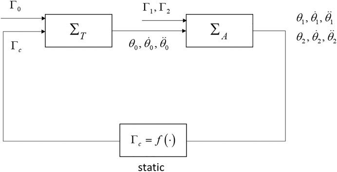
FIGURE 2. S3S decomposed model (${\Sigma }_T$ and ${\Sigma }_A$).

From where a state representation is:

$\begin{array}{l}\left[\begin{array}{cccc}1& 0& 0& 0\\ 0& 1& 0& 0\\ 0& 0& p_3& p_4\cos \left(q_2\right)\\ 0& 0& p_4\cos \left(q_2\right)& p_5\end{array}\right]\left[\begin{array}{c}{\dot{\theta }}_1\\ {\dot{\theta }}_2\\ {\ddot{\theta }}_1\\ {\ddot{\theta }}_2\end{array}\right]=\left[\begin{array}{cccc}0& 0& 1& 0\\ 0& 0& 0& 1\\ 0& 0& 0& p_4\sin \left(q_2\right){\dot{\theta }}_2\\ 0& 0& -p_4\sin \left(q_2\right){\dot{\theta }}_1& 0\end{array}\right]\left[\begin{array}{c}{\theta }_1\\ {\theta }_2\\ {\dot{\theta }}_1\\ {\dot{\theta }}_2\end{array}\right]\\ +\left[\begin{array}{cc}0& 0\\ 0& 0\\ 1& -1\\ 0& 1\end{array}\right]\left[\begin{array}{c}{\mathrm{\Gamma }}_1\\ {\mathrm{\Gamma }}_2\end{array}\right]+\left[\begin{array}{c}0\\ 0\\ p_6\sin \left({\theta }_1\right)\\ p_7\sin \left({\theta }_2\right)\end{array}\right]+\left[\begin{array}{cc}0& 0\\ 0& 0\\ p_8\sin \left(q_1\right)& p_8\cos \left(q_1\right)\\ p_9\sin \left(q_1+q_2\right)& p_9\cos \left(q_1+q_2\right)\end{array}\right]\left[\begin{array}{c}{\dot{\theta }}_0^2\\ {\ddot{\theta }}_0\end{array}\right],\end{array}(23)$

and considering ${\theta }_A=\left[\begin{array}{c}{\theta }_1\\ {\theta }_2\end{array}\right]$ which represents the measured variables and $x_A=\left[\begin{array}{c}{\theta }_A\\ {\dot{\theta }}_A\end{array}\right]$, the full state including the non-measured speeds as:

$\begin{array}{l}\left[\begin{array}{cc}I& 0\\ 0& \left[\begin{array}{cc}{p}_3& p_4\cos \left(q_2\right)\\ p_4\cos \left(q_2\right)& p_5\end{array}\right]\end{array}\right]\left[\begin{array}{c}{\dot{\theta }}_A\\ {\ddot{\theta }}_A\end{array}\right]=\left[\begin{array}{cc}0& I\\ 0& \left[\begin{array}{cc}0& p_4\sin \left(q_2\right){\dot{\theta }}_2\\ -p_4\sin \left(q_2\right){\dot{\theta }}_1& 0\end{array}\right]\end{array}\right]\left[\begin{array}{c}{\theta }_A\\ {\dot{\theta }}_A\end{array}\right]\\ +\left[\begin{array}{c}0\\ \left[\begin{array}{cc}1& -1\\ 0& 1\end{array}\right]\end{array}\right]\left[\begin{array}{c}{\mathrm{\Gamma }}_1\\ {\mathrm{\Gamma }}_2\end{array}\right]+\left[\begin{array}{c}0\\ D_a\left({\theta }_A\right)\end{array}\right]+\left[\begin{array}{c}0\\ C\left({\theta }_A\right)\end{array}\right]\left[\begin{array}{c}{\dot{\theta }}_0^2\\ {\ddot{\theta }}_0\end{array}\right],\end{array}(24)$

where $D_a\left({\theta }_A\right)=\left[\begin{array}{c}{p}_6\sin \left({\theta }_1\right)\\ p_7\sin \left({\theta }_2\right)\end{array}\right]$ and $C\left({\theta }_A\right)=\left[\begin{array}{cc}{p}_8\sin \left(q_1\right)& p_8\cos \left(q_1\right)\\ p_9\sin \left(q_1+q_2\right)& p_9\cos \left(q_1+q_2\right)\end{array}\right]$.

Finally, the static coupling term, Figure 2, that feedbacks from ${\Sigma }_A$ to ${\Sigma }_T$ corresponds to the following:

${\mathrm{\Gamma }}_c=\left[\begin{array}{cccc}-p_{10}\sin \left(q_1\right){\dot{\theta }}_1& -p_9\sin \left(q_1+q_2\right){\dot{\theta }}_2& p_{10}\cos \left(q_1\right)& p_9\cos \left(q_1+q_2\right)\end{array}\right]\left[\begin{array}{c}{\dot{\theta }}_1\\ {\dot{\theta }}_2\\ {\ddot{\theta }}_1\\ {\ddot{\theta }}_2\end{array}\right]-{\mathrm{\Gamma }}_1.(25)$

Thus, ${\Sigma }_A$ equation 21, ${\Sigma }_T$ (24) and the coupling term (25) exactly represent the S3S model (3).

Unknown Input Observation Problem

In both cases, as previously done for the S3S model (6), a double integrator cascade, that is, ${\ddot{\mathrm{\Gamma }}}_k\approx 0$ $k\in \left\{\mathrm{0,1,2}\right\}$ is used as a good compromise to realize the torque estimations. For the system ${\Sigma }_T$, the state is augmented to include the torque ${\mathrm{\Gamma }}_U={\mathrm{\Gamma }}_c+{\mathrm{\Gamma }}_0$. Effectively, at this first stage, there is no way to make a difference between the torques ${\mathrm{\Gamma }}_c$ and ${\mathrm{\Gamma }}_0$ as they enter at the same place in (20). Therefore, (21) is rewritten in the PI-extended form as:

$\left[\begin{array}{cc}\left[\begin{array}{cc}1& 0\\ 0& p_1\end{array}\right]& 0\\ 0& I\end{array}\right]\left[\begin{array}{c}{\dot{\theta }}_0\\ {\ddot{\theta }}_0\\ {\dot{\Omega }}_T\end{array}\right]=\left[\begin{array}{cc}\left[\begin{array}{cc}0& 1\\ p_2\frac{\sin \left({\theta }_0\right)}{{\theta }_0}& 0\end{array}\right]& \left[\begin{array}{cc}B& 0\end{array}\right]\\ 0& J\end{array}\right]\left[\begin{array}{c}{\theta }_0\\ {\dot{\theta }}_0\\ {\Omega }_T\end{array}\right],{\Omega }_T=\left[\begin{array}{c}{\mathrm{\Gamma }}_U\\ {\dot{\mathrm{\Gamma }}}_U\end{array}\right],J=\left[\begin{array}{cc}0& 1\\ 0& 0\end{array}\right].(26)$

For the model ${\Sigma }_A$ (24), the state is augmented to include the torques ${\mathrm{\Gamma }}_1$ and ${\mathrm{\Gamma }}_2$. For sake of simplification, we define $A_A\left(x_A\right)=\left[\begin{array}{cc}0& I\\ 0& \left[\begin{array}{cc}0& p_4\sin \left(q_2\right){\dot{\theta }}_2\\ -p_4\sin \left(q_2\right){\dot{\theta }}_1& 0\end{array}\right]\end{array}\right]$, $B_A=\left[\begin{array}{cc}0& 0\\ \left[\begin{array}{cc}1& -1\\ 0& 1\end{array}\right]& 0\end{array}\right]$, and $E_A\left({\theta }_2\right)=\left[\begin{array}{cc}I& 0\\ 0& \left[\begin{array}{cc}{p}_3& p_4\cos \left(q_2\right)\\ p_4\cos \left(q_2\right)& p_5\end{array}\right]\end{array}\right]$ to rewrite (24) as:

$E_A\left({\theta }_A\right){\dot{x}}_A=A_A\left(x_A\right)x_A+\left[\begin{array}{c}0\\ B\end{array}\right]\left[\begin{array}{c}{\mathrm{\Gamma }}_1\\ {\mathrm{\Gamma }}_2\end{array}\right]+\left[\begin{array}{c}0\\ D_a\left({\theta }_A\right)\end{array}\right]+\left[\begin{array}{c}0\\ C\left({\theta }_A\right)\end{array}\right]\left[\begin{array}{c}{\dot{\theta }}_0^2\\ {\ddot{\theta }}_0\end{array}\right],(27)$

and its extended PI-extended form with $J_2=\left[\begin{array}{cc}0& I_2\\ 0& 0\end{array}\right]$ and ${\Omega }_A={\left[\begin{array}{cccc}{\mathrm{\Gamma }}_1& {\dot{\mathrm{\Gamma }}}_1& {\mathrm{\Gamma }}_2& {\dot{\mathrm{\Gamma }}}_2\end{array}\right]}^T$ as:

$\{\begin{array}{l}\left[\begin{array}{cc}{E}_A\left({\theta }_2\right)& 0\\ 0& I\end{array}\right]\left[\begin{array}{c}{\dot{x}}_A\\ {\dot{\Omega }}_A\end{array}\right]=\left[\begin{array}{cc}{A}_A\left(x_A\right)& B_A\\ 0& J_2\end{array}\right]\left[\begin{array}{c}{x}_A\\ {\Omega }_A\end{array}\right]+\left[\begin{array}{c}0\\ D_a\left({\theta }_A\right)\\ 0\end{array}\right]+\left[\begin{array}{c}0\\ C\left({\theta }_A\right)\\ 0\end{array}\right]\left[\begin{array}{c}{\dot{\theta }}_0^2\\ {\ddot{\theta }}_0\end{array}\right]\\ y_A=\left[\begin{array}{cc}{I}_2& 0\end{array}\right]\left[\begin{array}{c}{x}_A\\ {\Omega }_A\end{array}\right]={\theta }_A=\left[\begin{array}{c}{\theta }_1\\ {\theta }_2\end{array}\right]\end{array}.(28)$

Thus, with (26), (28), and the coupling term (25), the goal is to build a cascade of two observers for ${\Sigma }_T$ and ${\Sigma }_A$, and to make their synthesis in order to guarantee an asymptotic convergence as well as performances comparable to a global observer. Before solving the problem for the S3S model, let us give a general result concerning cascade observers in the descriptor form.

Cascade Observation Problem

Conditions for a Separation Principle

Cascade observation has been studied for interconnected non-linear and linear systems, for example in Lendek et al. (2008), Gripa et al. (2012). The idea is to build observers independently, in a way that the global performances are satisfied. Thus, we can combine different types of observer regarding the local subsystem concerned. A separation principle is proposed based on a vector comparison principle, and the proof follows similar paths than the observer/control separation principle for quasi-LPV systems (Ma et al., 1998). The advantage of this methodology of estimation is that separate observers can be built from a local subsystem which makes their adjustment less difficult (Lendek, et al., 2010).

Consider the following proposition.

Theorem 1: consider two descriptor systems $\left[E_i(\cdot ),A_i(\cdot ),C_i(\cdot )\right]$, $i\in \left\{\mathrm{1,2}\right\}$ ($E_i(\cdot )$ being always regular) such that it exists in matrices as $K_i(\cdot )$, $i\in \left\{\mathrm{1,2}\right\}$ ensuring that the estimation error systems defined by $E_i(\cdot ){\dot{e}}_i=\left[A_i(\cdot )-K_i(\cdot )C_i(\cdot )\right]e_i$ are globally asymptotically stable (GAS); knowing it exists as two Lyapunov functions $V_i\left(e_i\right)$ and scalars ${\overline{\lambda }}_i\ge {\underset{¯}{\lambda }}_i>0$, ${\mu }_i>0$, ${\delta }_i>0$ satisfying the following:

$0<{\underset{¯}{\lambda }}_i{\Vert e_i\Vert }^2\le V_i\left(e_i\right)\le {\overline{\lambda }}_i{\Vert e_i\Vert }^2.(29)$

$\frac{\partial V_i\left(e_i\right)}{\partial e_i}{\dot{e}}_i=\frac{\partial V_i\left(e_i\right)}{\partial e_i}{E}_i^{-1}(\cdot )\left(A_i(\cdot )-K_i(\cdot )C_i(\cdot )\right)\le -{\mu }_i{\Vert e_i\Vert }^2.(30)$

$\Vert \frac{\partial V_i\left(e_i\right)}{\partial e_i}\Vert \le {\delta }_i{\Vert e_i\Vert }^2.(31)$

Consider the System

$\left[\begin{array}{cc}{E}_1(\cdot )& 0\\ E_{12}(\cdot )& E_2(\cdot )\end{array}\right]\dot{e}=\left[\begin{array}{cc}{A}_1(\cdot )-K_1(\cdot )C_1(\cdot )& 0\\ A_{12}(\cdot )& A_2(\cdot )-K_2(\cdot )C_2(\cdot )\end{array}\right]e,(32)$

where $E_{12}(\cdot )$ and $A_{12}(\cdot )$ norm-bounded; then (32) is also globally asymptotically stable.

 Proof: $E_i(\cdot )$ being regular, it is direct that ${\left[\begin{array}{cc}{E}_1(\cdot )& 0\\ E_{12}(\cdot )& E_2(\cdot )\end{array}\right]}^{-1}=\left[\begin{array}{cc}{E}_1^{-1}(\cdot )& 0\\ -E_2^{-1}(\cdot )E_{12}(\cdot )E_1^{-1}(\cdot )& E_2^{-1}(\cdot )\end{array}\right]$; let us rewrite $A_i^{\ast }(\cdot )=E_i^{-1}(\cdot )\left(A_i(\cdot )-K_i(\cdot )C_i(\cdot )\right)$, thus (32) is equivalent to the following:

$\dot{e}=\left[\begin{array}{cc}{A}_1^{\ast }(\cdot )& 0\\ E_2^{-1}(\cdot )\left(A_{12}(\cdot )-E_{12}(\cdot )A_1^{\ast }(\cdot )\right)& A_2^{\ast }(\cdot )\end{array}\right]e.(33)$

Consider now a positive scalar $\gamma >0$ and the Lyapunov function as:

$V\left(e_1,e_2\right)=V_1\left(e_1\right)+\gamma V_2\left(e_2\right).(34)$

Its derivative along the trajectories of (33) is:

$\begin{array}{l}\dot{V}\left(e_1,e_2\right)=\frac{\partial V_1\left(e_1\right)}{\partial e_1}{\dot{e}}_1+\gamma \frac{\partial V_2\left(e_2\right)}{\partial e_2}{\dot{e}}_2\\ =\frac{\partial V_1\left(e_1\right)}{\partial e_1}{A}_1^{\ast }(\cdot )e_1+\gamma \frac{\partial V_2\left(e_2\right)}{\partial e_2}{A}_2^{\ast }(\cdot )e_2+\gamma \frac{\partial V_2\left(e_2\right)}{\partial e_2}{E}_2^{-1}(\cdot )\left(A_{12}(\cdot )-E_{12}(\cdot )A_1^{\ast }(\cdot )\right)e_1.\end{array}(35)$

Using (30) and Passing at Norms, we get the following:

$\dot{V}\left(e_1,e_2\right)\le -{\mu }_1{\Vert e_1\Vert }^2-\gamma {\mu }_2{\Vert e_2\Vert }^2+\gamma \Vert \frac{\partial V_2\left(e_2\right)}{\partial e_2}\Vert \Vert E_2^{-1}(\cdot )\left(A_{12}(\cdot )-E_{12}(\cdot )A_1^{\ast }(\cdot )\right)\Vert \Vert e_1\Vert ,(36)$

where $A_1^{\ast }(\cdot )$ is GAS, and $E_{12}(\cdot )$ and $A_{12}(\cdot )$ are norm-bounded; we can write that it exists a positive scalar $M>0$ such that $\Vert E_2^{-1}(\cdot )\left(A_{12}(\cdot )-E_{12}(\cdot )A_1^{\ast }(\cdot )\right)\Vert \le M$. Using condition (31), the bound (36) of the derivative $\dot{V}\left(e_1,e_2\right)$ holds if:

$\dot{V}\left(e_1,e_2\right)\le -{\mu }_1{\Vert e_1\Vert }^2-\gamma {\mu }_2{\Vert e_2\Vert }^2+\gamma {\delta }_{2}M\Vert e_1\Vert \Vert e_2\Vert .(37)$

Using a completion of square, (37) is equivalent to:

$\dot{V}\left(e_1,e_2\right)\le -\left({\mu }_1-\gamma \frac{{\delta }_2^2{M}^2}{4{\mu }_2}\right){\Vert e_1\Vert }^2-\gamma {\left(\sqrt{{\mu }_2}\Vert e_2\Vert -\frac{{\delta }_{2}M}{2\sqrt{{\mu }_2}}\Vert e_1\Vert \right)}^2.(38)$

As $\gamma >0$ is a free parameter, it can always be set such as $\gamma <\frac{4{\mu }_1{\mu }_2}{{\delta }_2^2{M}^2}$ and thus, $\dot{V}\left(e_1,e_2\right)<0$ $\forall \left(e_1,e_2\right)\ne 0$ which ends the proof.Remark 4: This result is readily extended to a n-cascade of observers that keep the triangular structure of (32) and the norm-bounded property on its non-diagonal entries. This will be particularly interesting for the future studies considering a 3D-S3S model.From this general result, next part shows how to exploit it to derive the 2D-S3S cascaded observers via LMI constraints problems.

Cascade Proportional Integral-Observers for the S3S Model

First of all, let us describe the two observers cascade for the S3S case, Figure 3. Recall that only the angles are measured. Thus the first observer of ${\Sigma }_T$ (so-called ${\widehat{\Sigma }}_T$, Figure 3) has ${\theta }_0$ and ${\dot{\widehat{\theta }}}_0$ as inputs, and ${\widehat{\mathrm{\Gamma }}}_U={\widehat{\mathrm{\Gamma }}}_c+{\widehat{\mathrm{\Gamma }}}_0$ as output. The second observer for ${\Sigma }_A$ (so-called ${\widehat{\Sigma }}_A$, Figure 3) uses the first observer outputs and the angles ${\theta }_1$ and ${\theta }_2$ as inputs. Its outputs are ${\widehat{\theta }}_i$, ${\dot{\widehat{\theta }}}_i$, and ${\widehat{\mathrm{\Gamma }}}_i$ $i\in \left\{\mathrm{1,2}\right\}$.

FIGURE 3

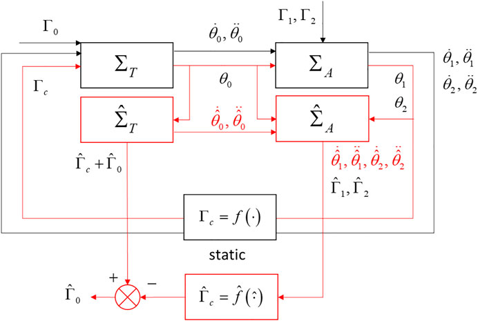
FIGURE 3. 2-observers cascade for the decomposed S3S model.

We considered the extended body trunk model ${\Sigma }_T$ (26) and transform it in a classical non-descriptor form with: x_T = $\left[\begin{array}{c}{\theta }_0\\ {\dot{\theta }}_0\end{array}\right],A_T\left({\theta }_0\right)=\left[\begin{array}{cc}1& 0\\ 0& p_1^{-1}\end{array}\right]\left[\begin{array}{cc}0& 1\\ p_2\frac{\sin \left({\theta }_0\right)}{{\theta }_0}& 0\end{array}\right],$ $B=\left[\begin{array}{c}0\\ 1\end{array}\right],$ $B_T=\left[\begin{array}{cc}1& 0\\ 0& p_1^{-1}\end{array}\right]\left[\begin{array}{cc}B& 0\end{array}\right],$ and $J=\left[\begin{array}{cc}0& 1\\ 0& 0\end{array}\right]$.

To get a compact form of (26):

$\left[\begin{array}{c}{\dot{x}}_T\\ {\dot{\Omega }}_T\end{array}\right]=\left[\begin{array}{cc}{A}_T\left({\theta }_0\right)& B_T\\ 0& J\end{array}\right]\left[\begin{array}{c}{x}_T\\ {\Omega }_T\end{array}\right].(39)$

Therefore, we considered a first local observer for ${\Sigma }_T$:

$\left[\begin{array}{c}{\dot{\widehat{x}}}_T\\ {\dot{\widehat{\Omega }}}_T\end{array}\right]=\left[\begin{array}{cc}{A}_T\left({\theta }_0\right)& B_T\\ 0& J\end{array}\right]\left[\begin{array}{c}{\widehat{x}}_T\\ {\widehat{\Omega }}_T\end{array}\right]+K_T\left({\theta }_0\right)\left(y_T-{\widehat{y}}_T\right),{\widehat{y}}_T=C_T{\widehat{x}}_T={\theta }_0,(40)$

and the estimation error dynamic $e_T=\left[\begin{array}{c}{x}_T\\ {\Omega }_T\end{array}\right]-\left[\begin{array}{c}{\widehat{x}}_T\\ {\widehat{\Omega }}_T\end{array}\right]$ writes as:

${\dot{e}}_T=\left(\left[\begin{array}{cc}{A}_T\left({\theta }_0\right)& B_T\\ 0& J\end{array}\right]-K_T\left({\theta }_0\right)C_T\right)e_T,(41)$

The design of $K_T\left({\theta }_0\right)$ such that (41) is GAS is explained in section PI-Observers Cascade Design.

For the extended shoulder and the arm system ${\Sigma }_A$ (28), the observer can be derived paying attention that ${\dot{\theta }}_0$ and ${\ddot{\theta }}_0$ being non-measured, they are replaced with their estimate ${\dot{\widehat{\theta }}}_0$ and ${\ddot{\widehat{\theta }}}_0$. Thus, an expression is:

$\left[\begin{array}{cc}{E}_A\left({\theta }_2\right)& 0\\ 0& I\end{array}\right]\left[\begin{array}{c}{\dot{\widehat{x}}}_A\\ {\dot{\widehat{\Omega }}}_A\end{array}\right]=\left[\begin{array}{cc}{A}_A\left({\widehat{x}}_A\right)& B_A\\ 0& J_2\end{array}\right]\left[\begin{array}{c}{\widehat{x}}_A\\ {\widehat{\Omega }}_A\end{array}\right]+\left[\begin{array}{c}0\\ D_a\left({\theta }_A\right)\\ 0\end{array}\right]+\left[\begin{array}{c}0\\ C\left({\theta }_A\right)\\ 0\end{array}\right]\left[\begin{array}{c}{\dot{\widehat{\theta }}}_0^2\\ {\ddot{\widehat{\theta }}}_0\end{array}\right]+K_A(\cdot )\left(y_A-{\widehat{y}}_A\right).(42)$

Let us define the observation error $e_A=\left[\begin{array}{c}{x}_A\\ {\Omega }_A\end{array}\right]-\left[\begin{array}{c}{\widehat{x}}_A\\ {\widehat{\Omega }}_A\end{array}\right]$ and writing $\left[\begin{array}{cc}{E}_A\left({\theta }_2\right)& 0\\ 0& I\end{array}\right]{\dot{e}}_A$ renders as: $\left[\begin{array}{cc}{E}_A\left({\theta }_2\right)& 0\\ 0& I\end{array}\right]{\dot{e}}_A=\left[\begin{array}{cc}{A}_A\left(x_A\right)& B_A\\ 0& J_2\end{array}\right]\left[\begin{array}{c}{x}_A\\ {\Omega }_A\end{array}\right]-\left[\begin{array}{cc}{A}_A\left({\widehat{x}}_A\right)& B_A\\ 0& J_2\end{array}\right]\left[\begin{array}{c}{\widehat{x}}_A\\ {\widehat{\Omega }}_A\end{array}\right]-K_A(\cdot )C{e}_A+\left[\begin{array}{c}0\\ C\left({\theta }_A\right)\\ 0\end{array}\right]\left(\left[\begin{array}{c}{\dot{\theta }}_0^2\\ {\ddot{\theta }}_0\end{array}\right]-\left[\begin{array}{c}{\dot{\widehat{\theta }}}_0^2\\ {\ddot{\widehat{\theta }}}_0\end{array}\right]\right)$

From where defining $\Delta A_A(\cdot )=A_A\left(x_A\right)-A_A\left({\widehat{x}}_A\right)$ and $\Delta {\theta }_T=\left[\begin{array}{c}{\dot{\theta }}_0^2\\ {\ddot{\theta }}_0\end{array}\right]-\left[\begin{array}{c}{\dot{\widehat{\theta }}}_0^2\\ {\ddot{\widehat{\theta }}}_0\end{array}\right]$ as:

$\left[\begin{array}{cc}{E}_A\left({\theta }_2\right)& 0\\ 0& I\end{array}\right]{\dot{e}}_A=\left(\left[\begin{array}{cc}{A}_A\left(x_A\right)& B_A\\ 0& J_2\end{array}\right]-K_A(\cdot )C\right)e_A+\left[\begin{array}{c}\Delta A_A(\cdot ){\widehat{x}}_A\\ 0\end{array}\right]+\left[\begin{array}{c}0\\ C\left({\theta }_A\right)\\ 0\end{array}\right]\left(\left[\begin{array}{c}{\dot{\theta }}_0^2\\ {\ddot{\theta }}_0\end{array}\right]-\left[\begin{array}{c}{\dot{\widehat{\theta }}}_0^2\\ {\ddot{\widehat{\theta }}}_0\end{array}\right]\right).(43)$

Now, in order to apply the result of Theorem 1, (43) must be adequately written as the second row of (32). The last part of (43) writes as: $\left[\begin{array}{c}{\dot{\theta }}_0^2\\ {\ddot{\theta }}_0\end{array}\right]-\left[\begin{array}{c}{\dot{\widehat{\theta }}}_0^2\\ {\ddot{\widehat{\theta }}}_0\end{array}\right]=\left[\begin{array}{cc}{\dot{\theta }}_0+{\dot{\widehat{\theta }}}_0& 0\\ 0& 1\end{array}\right]\left[\begin{array}{c}{\dot{\theta }}_0-{\dot{\widehat{\theta }}}_0\\ {\ddot{\theta }}_0-{\ddot{\widehat{\theta }}}_0\end{array}\right]$ from where:

$\left[\begin{array}{c}0\\ C\left({\theta }_A\right)\\ 0\end{array}\right]\left(\left[\begin{array}{c}{\dot{\theta }}_0^2\\ {\ddot{\theta }}_0\end{array}\right]-\left[\begin{array}{c}{\dot{\widehat{\theta }}}_0^2\\ {\ddot{\widehat{\theta }}}_0\end{array}\right]\right)=\left[\begin{array}{c}0\\ C\left({\theta }_A\right)\\ 0\end{array}\right]\left[\begin{array}{ccc}{\dot{\theta }}_0+{\dot{\widehat{\theta }}}_0& 0& 0\\ 0& 1& 0\end{array}\right]\left[\begin{array}{c}{\dot{\theta }}_0-{\dot{\widehat{\theta }}}_0\\ {\ddot{\theta }}_0-{\ddot{\widehat{\theta }}}_0\\ {\Omega }_T-{\widehat{\Omega }}_T\end{array}\right]=-E_{12}\left({\theta }_A,{\dot{\theta }}_0,{\dot{\widehat{\theta }}}_0\right){\dot{e}}_T,(44)$

where $E_{12}\left({\theta }_A,{\dot{\theta }}_0,{\dot{\widehat{\theta }}}_0\right)=-\left[\begin{array}{c}0\\ C\left({\theta }_A\right)\\ 0\end{array}\right]\left[\begin{array}{ccc}{\dot{\theta }}_0+{\dot{\widehat{\theta }}}_0& 0& 0\\ 0& 1& 0\end{array}\right]$. The last transformation concerns the middle term of (43). Considering that $\Delta A_A(\cdot )=p_4\sin \left(q_2\right)\left[\begin{array}{cc}0& 0\\ 0& \left[\begin{array}{cc}0& {\dot{\theta }}_2-{\dot{\widehat{\theta }}}_2\\ -{\dot{\theta }}_1+{\dot{\widehat{\theta }}}_1& 0\end{array}\right]\end{array}\right]$, let us rewrite the part $A_A\left(x_A\right)e_A+\Delta A_A(\cdot ){\widehat{x}}_A$ in (43) such as:

$A_A\left(x_A\right)e_A+\Delta A_A(\cdot ){\widehat{x}}_A=\left[\begin{array}{cc}0& I\\ 0& p_4\sin \left(q_2\right)\left[\begin{array}{cc}0& {\dot{\theta }}_2+{\dot{\widehat{\theta }}}_2\\ -{\dot{\theta }}_1-{\dot{\widehat{\theta }}}_1& 0\end{array}\right]\end{array}\right]e_A=H\left(x_A,{\widehat{x}}_A\right)e_A.(45)$

Finally, (43) can be transformed in the following:

$E_{12}\left({\theta }_A,{\dot{\theta }}_0,{\dot{\widehat{\theta }}}_0\right){\dot{e}}_T+\left[\begin{array}{cc}{E}_A\left({\theta }_2\right)& 0\\ 0& I\end{array}\right]{\dot{e}}_A=\left(\left[\begin{array}{cc}H\left(x_A,{\widehat{x}}_A\right)& B_A\\ 0& J_2\end{array}\right]-K_A(\cdot )C\right)e_A,(46)$

and the full observation problem writes from (41) and (46) as:

$\left[\begin{array}{cc}I& 0\\ E_{12}(\cdot )& \left[\begin{array}{cc}{E}_A\left({\theta }_2\right)& 0\\ 0& I\end{array}\right]\end{array}\right]\left[\begin{array}{c}{\dot{e}}_T\\ {\dot{e}}_A\end{array}\right]=\left[\begin{array}{cc}\left[\begin{array}{cc}{A}_T\left({\theta }_0\right)& B_T\\ 0& J\end{array}\right]-K_T\left({\theta }_0\right)C_T& 0\\ 0& \left[\begin{array}{cc}H\left(x_A,{\widehat{x}}_A\right)& B_A\\ 0& J_2\end{array}\right]-K_A(\cdot )C\end{array}\right]\left[\begin{array}{c}{e}_T\\ e_A\end{array}\right].(47)$

Eq. (47) does correspond to the conditions of Theorem 1, the non-diagonal terms being bounded. Thus, conditions of Theorem one are fulfilled and the separation principle applies.

Proportional Integral-Observers Cascade Design

Proportional Integral-Observer for ${\Sigma }_{\mathit{T}}$

The first observer (40) for the body trunk model ${\Sigma }_T$ is associated with the error dynamic model (41) recalled thereafter:

${\dot{e}}_T=\left(\left[\begin{array}{cc}{A}_T\left({\theta }_0\right)& B_T\\ 0& J\end{array}\right]-K_T\left({\theta }_0\right)C_T\right)e_T.(48)$

As $A_T\left({\theta }_0\right)=\left[\begin{array}{cc}0& 1\\ \beta p_1^{-1}{p}_2\frac{\sin \left({\theta }_0\right)}{{\theta }_0}& 0\end{array}\right]$ and $C_T=\left[\begin{array}{cccc}1& 0& 0& 0\end{array}\right]$, consider the following observer gain: $K_T\left({\theta }_0\right)={\left[\begin{array}{cccc}0& \beta p_1^{-1}{p}_2\frac{\sin \left({\theta }_0\right)}{{\theta }_0}& 0& 0\end{array}\right]}^T+K_{LT}$, $K_{LT}\in {ℝ}^{4\times 1}$. Thus, the observation error is linear:

${\dot{e}}_T=\left(\left[\begin{array}{cc}J& B_T\\ 0& J\end{array}\right]-K_{LT}{C}_T\right)e_T.(49)$

Any method can come at hand to determine $K_{LT}$. Therefore, the observer writes as:

$\left[\begin{array}{c}{\dot{\widehat{x}}}_T\\ {\dot{\widehat{\Omega }}}_T\end{array}\right]=\left[\begin{array}{cc}{A}_T\left({\theta }_0\right)& B_T\\ 0& J\end{array}\right]\left[\begin{array}{c}{\widehat{x}}_T\\ {\widehat{\Omega }}_T\end{array}\right]-\left({\left[\begin{array}{cccc}0& \beta p_1^{-1}{p}_2\frac{\sin \left({\theta }_0\right)}{{\theta }_0}& 0& 0\end{array}\right]}^T+K_{LT}\right)\left(y_T-{\widehat{y}}_T\right).(50)$

Proportional Integral-Observer for ${\Sigma }_A$

The second observer (42) for the model ${\Sigma }_A$ is associated with a reduced error dynamic model issued from (46), with $H\left(x_A,{\widehat{x}}_A\right)$ given in (45):

$\left[\begin{array}{cc}{E}_A\left({\theta }_2\right)& 0\\ 0& I\end{array}\right]{\dot{\epsilon }}_A=\left(\left[\begin{array}{cc}H\left(x_A,{\widehat{x}}_A\right)& B_A\\ 0& J_2\end{array}\right]-K_A(\cdot )C\right){\epsilon }_A.(51)$

In (51), it appears ${\epsilon }_A$ as a slack variable different from $e_A$, as it is not the full-term error on the ${\Sigma }_A$ model. Thus, from the separation principle result if (41) and (51) are GAS, (47) is GAS.

The non-linear model (51) has a non-linear part $E_A\left({\theta }_2\right)$ on the left. Of course as $E_A^{-1}\left({\theta }_2\right)$ exists for every ${\theta }_2$ a classic representation of (51) could be used. Nevertheless, see Remark 1, a descriptor form is kept and the a polytopic representation of (51) is derived. $E_A\left({\theta }_2\right)$ has one non-linearity $\cos \left(q_2\right)$, and $H\left(x_A,{\widehat{x}}_A\right)$ defined in (45) two non-linearities: $\sin \left(q_2\right)\left({\dot{\theta }}_1+{\dot{\widehat{\theta }}}_1\right)$ and $\sin \left(q_2\right)\left({\dot{\theta }}_2+{\dot{\widehat{\theta }}}_2\right)$. Therefore, a $2^3=8$ vertices corresponding to a polytopic model can be derived as:

${\displaystyle \sum _{i=1}^2{v}_i\left(q_2\right)\left[\begin{array}{cc}{E}_{Ai}& 0\\ 0& I\end{array}\right]{\dot{\epsilon }}_A}={\displaystyle \sum _{i=1}^2{\displaystyle \sum _{j=1}^2{w}_{1i}\left(x_A,{\widehat{x}}_A\right)w_{2j}\left(x_A,{\widehat{x}}_A\right)\left(\left[\begin{array}{cc}{H}_{ij}& B_A\\ 0& J_2\end{array}\right]-K_A(\cdot )C\right){\epsilon }_A}},(52)$

with $\cos \left(q_2\right)\in \left[v,1\right]$, $v_1\left(q_2\right)=\frac{1-\cos \left(q_2\right)}{1-v}=1-v_2\left(q_2\right)$, $\sin \left(q_2\right)\left({\dot{\theta }}_i+{\dot{\widehat{\theta }}}_i\right)\in \left[{\underset{¯}{\rho }}_i,{\overline{\rho }}_i\right]$, $i\in \left\{\mathrm{1,2}\right\}$ $w_{i1}\left(x_A,{\widehat{x}}_A\right)=\frac{{\overline{\rho }}_i-\sin \left(q_2\right)\left({\dot{\theta }}_i+{\dot{\widehat{\theta }}}_i\right)}{{\overline{\rho }}_i-{\underset{¯}{\rho }}_i}=1-w_{i2}\left(x_A,{\widehat{x}}_A\right)$, $i\in \left\{\mathrm{1,2}\right\}$ and the matrices:

$\begin{array}{l}{E}_{A1}=\left[\begin{array}{cc}I& 0\\ 0& \left[\begin{array}{cc}{p}_3& v{p}_4\\ v{p}_4& p_5\end{array}\right]\end{array}\right],E_{A2}=\left[\begin{array}{cc}I& 0\\ 0& \left[\begin{array}{cc}{p}_3& p_4\\ p_4& p_5\end{array}\right]\end{array}\right],H_{11}=\left[\begin{array}{cc}0& I\\ 0& p_4\left[\begin{array}{cc}0& {\underset{¯}{\rho }}_2\\ -{\underset{¯}{\rho }}_1& 0\end{array}\right]\end{array}\right],H_{21}=\left[\begin{array}{cc}0& I\\ 0& p_4\left[\begin{array}{cc}0& {\underset{¯}{\rho }}_2\\ -{\overline{\rho }}_1& 0\end{array}\right]\end{array}\right],H_{12}=\left[\begin{array}{cc}0& I\\ 0& p_4\left[\begin{array}{cc}0& {\overline{\rho }}_2\\ -{\underset{¯}{\rho }}_1& 0\end{array}\right]\end{array}\right],\mathrm{a}\mathrm{n}\mathrm{d}{H}_{22}=\left[\begin{array}{cc}0& I\\ 0& p_4\left[\begin{array}{cc}0& {\overline{\rho }}_2\\ -{\overline{\rho }}_1& 0\end{array}\right]\end{array}\right].\end{array}(53)$

From this polytopic description, as usual, an extended description of (52) is used (Taniguchi et al., 2000). The extended state ${\epsilon }^{\ast }=\left[\begin{array}{c}{\epsilon }_A\\ {\dot{\epsilon }}_A\end{array}\right]$ is chosen together using $\overline{E}=\left[\begin{array}{cc}I& 0\\ 0& 0\end{array}\right]$ and with a Lyapunov function:

$V\left({\epsilon }^{\ast }\right)={\epsilon }^{\ast T}{\overline{E}}^{T}P{\epsilon }^{\ast },P=\left[\begin{array}{cc}{P}_1& 0\\ P_3& P_4\end{array}\right],P_1=P_1^T\succ 0.(54)$

The observer gain can only depend on measured variables; therefore, due to the definitions of $w_{i1}i,j\in \left\{\mathrm{1,2}\right\}$, only $v_i\left(q_2\right)$ is concerned:

$\overline{E}{\dot{\epsilon }}^{\ast }=\left({\overline{A}}_{v{w}_1{w}_2}-P^{-T}{\overline{K}}_v\overline{C}\right){\epsilon }^{\ast },(55)$

with ${\overline{A}}_{v{w}_1{w}_2}=\left[\begin{array}{cc}0& I\\ \left[\begin{array}{cc}{H}_{w_1{w}_2}& B_A\\ 0& J_2\end{array}\right]& -[\begin{array}{cc}{E}_{Av}& 0\\ 0& I\end{array}\end{array}\right]]$ and ${\overline{K}}_v=\left[\begin{array}{c}{K}_{1v}\\ K_{2v}\end{array}\right]$. Following the study of Guerra et al. (2015), a LMI constraint problem is given by the following:

Find $P=\left[\begin{array}{cc}{P}_1& 0\\ P_3& P_4\end{array}\right],P_1=P_1^T\succ 0$, $\left[\begin{array}{c}{K}_{1i}\\ K_{2i}\end{array}\right]$ such that, $i,j,k\in \left\{\mathrm{1,2}\right\}$

$\left[\begin{array}{cc}{P}_3^T\left[\begin{array}{cc}{H}_{jk}& B_A\\ 0& J_2\end{array}\right]-K_{1i}C+(\ast )& (\ast )\\ P_4^T\left[\begin{array}{cc}{H}_{jk}& B_A\\ 0& J_2\end{array}\right]-K_{2i}C+P_1-{\left[\begin{array}{cc}{E}_{Ai}& 0\\ 0& I\end{array}\right]}^T{P}_3& -P_4^T\left[\begin{array}{cc}{E}_{Ai}& 0\\ 0& I\end{array}\right]-{\left[\begin{array}{cc}{E}_{Ai}& 0\\ 0& I\end{array}\right]}^T{P}_4\end{array}\right]<0.(56)$

At the end, the observer for ${\Sigma }_A$ is, with $P=\left[\begin{array}{cc}{P}_1& 0\\ P_3& P_4\end{array}\right],P_1=P_1^T\succ 0$, $\left[\begin{array}{c}{K}_{1i}\\ K_{2i}\end{array}\right]$ $i\in \left\{\mathrm{1,2}\right\}$, solution of, (56):

$\begin{array}{c}{\displaystyle \sum _{i=1}^2{v}_i\left(q_2\right)\left[\begin{array}{cc}{E}_{Ai}& 0\\ 0& I\end{array}\right]}\left[\begin{array}{c}{\dot{\widehat{x}}}_A\\ {\dot{\widehat{\Omega }}}_A\end{array}\right]=\left[\begin{array}{cc}{A}_A\left({\widehat{x}}_A\right)& B_A\\ 0& J_2\end{array}\right]\left[\begin{array}{c}{\widehat{x}}_A\\ {\widehat{\Omega }}_A\end{array}\right]+\left[\begin{array}{c}0\\ D_a\left({\theta }_A\right)\\ 0\end{array}\right]+\left[\begin{array}{c}0\\ C\left({\theta }_A\right)\\ 0\end{array}\right]\left[\begin{array}{c}{\dot{\widehat{\theta }}}_0^2\\ {\ddot{\widehat{\theta }}}_0\end{array}\right]\\ +\left[\begin{array}{cc}{\displaystyle \sum _{i=1}^2{v}_i\left(q_2\right)\left[\begin{array}{cc}{E}_{Ai}& 0\\ 0& I\end{array}\right]}& I\end{array}\right]P_{(\cdot )}^{-T}{\displaystyle \sum _{i=1}^2{v}_i\left(q_2\right)\left[\begin{array}{c}{K}_{1i}(\cdot )\\ K_{2i}(\cdot )\end{array}\right]}\left(y_A-{\widehat{y}}_A\right).\end{array}(57)$

At last for the coupling term ${\mathrm{\Gamma }}_c$ (25):

${\widehat{\mathrm{\Gamma }}}_c=\left[\begin{array}{cccc}-p_{10}\sin \left(q_1\right){\dot{\widehat{\theta }}}_1& -p_9\sin \left(q_1+q_2\right){\dot{\widehat{\theta }}}_2& p_{10}\cos \left(q_1\right)& p_9\cos \left(q_1+q_2\right)\end{array}\right]\left[\begin{array}{c}{\dot{\widehat{x}}}_A\\ {\dot{\widehat{\Omega }}}_A\end{array}\right]-{\widehat{\mathrm{\Gamma }}}_1.(58)$

Linear Matrix Inequalities Solutions

For the global continuous PI-observer, solving the LMI constraints problem (18) in the compact set ${\Omega }_x$ (17) is feasible. To enhance the performances, a decay rate (add $\tau P_1$, $\tau >0$ in the first entry of constraints (18)) and a norm limitation on the gains $\left[\begin{array}{cc}{K}_{1i}& K_{2i}\end{array}\right]\left[\begin{array}{c}{K}_{1i}\\ K_{2i}\end{array}\right]\le \epsilon I_3$ are used. The second part, using a Schur’s complement being equivalent to $\left[\begin{array}{cc}\epsilon I_3& \left[\begin{array}{cc}{K}_{1i}& K_{2i}\end{array}\right]\\ \left[\begin{array}{c}{K}_{1i}\\ K_{2i}\end{array}\right]& I_{24}\end{array}\right]\ge 0$. A good compromise was obtained using a decay rate of $\tau =6$ and $\epsilon ={10}^6$. It is useless to present the full set of matrices solution of the problem, just the extreme of the polytope of the gains $K_{\mathrm{2,1}}$ and $K_{\mathrm{2,16}}$ are given to exemplify:

$K_{\mathrm{2,1}}=\left[\begin{array}{ccc}71\text{.}1& 4\text{.}3& -2.2\\ -\text{0}\text{.}5& 111& -33\\ -2.9& -35.3& 222\\ 79& 12& -2\\ 10.5& 45.4& 12\\ 1.7& 13.4& 1.1\\ -1.6& 1.4& 0.01\\ -0.33& -12.3& -6\\ 1.9& -4.7& 8.5\\ 0& 0& 0\\ 0& 0& 0\\ 0& 0& 0\end{array}\right],K_{\mathrm{2,16}}=\left[\begin{array}{ccc}66.2& -0.7& -1.8\\ -2.3& 115& -36\\ -4.3& -35& 230\\ 83& 7.5& 3.8\\ 7.4& 50& 17.6\\ 2.8& 16.8& -2.2\\ -1.5& -1.6& -0.5\\ -7.7& -5.7& -9.5\\ 7.8& -7& 23\\ 0& 0& 0\\ 0& 0& 0\\ 0& 0& 0\end{array}\right].$

Local trunk observer gain $K_{LT}$ is easily calculated via pole placement, after some trials-and-errors. The solution of (49) for the model ${\Sigma }_T$ observer is: $K_{LT}={10}^2{\left[\begin{array}{cccc}6& 4& 5.4\times {10}^2& 1.9\times {10}^2\end{array}\right]}^T.$

For the problem (56), a decay rate of $\tau =7$ has been added in the first entry of (56), and the solution adopted by solving LMIs problem is $\left[\begin{array}{c}{K}_{1i}(\cdot )\\ K_{2i}(\cdot )\end{array}\right]$, $i\in \left\{\mathrm{1,2}\right\}$ where:

$\begin{array}{l}{K}_{11}=\left[\begin{array}{cc}141.2& -31.3\\ -31.3& 144.4\\ 11.8& -3\\ -3.6& 12.7\\ 8\times {10}^{-3}& 6\times {10}^{-3}\\ 3\times {10}^{-3}& -5\times {10}^{-3}\\ {10}^{-3}& 2\times {10}^{-3}\\ {10}^{-4}& -3\times {10}^{-3}\end{array}\right],K_{12}=\left[\begin{array}{cc}131.6& -27.1\\ -21.2& 122.6\\ 10.7& -2.7\\ -1.4& 9.8\times {10}^{-1}\\ 2\times {10}^{-3}& 4\times {10}^{-3}\\ 8\times {10}^{-3}& -3.3\times {10}^{-1}\\ {10}^{-3}& 9\times {10}^{-3}\\ {10}^{-4}& -21\times {10}^{-4}\end{array}\right],\\ K_{21}=\left[\begin{array}{cc}19.3& -4.5\\ -4.6& 20.1\\ -2.7\times {10}^{-1}& 92\times {10}^{-2}\\ -3.6\times {10}^{-2}& -18\times {10}^{-2}\\ 6\times {10}^{-4}& 49\times {10}^{-3}\\ 13\times {10}^{-4}& 8\times {10}^{-3}\\ {10}^{-4}& 2\times {10}^{-3}\\ {10}^{-3}& -3\times {10}^{-4}\end{array}\right],K_{22}=\left[\begin{array}{cc}15.3& -7.5\\ -4.98& 28.1\\ -2\times {10}^{-1}& 8.7\times {10}^{-1}\\ -2\times {10}^{-2}& -5\times {10}^{-2}\\ 8\times {10}^{-4}& 5\times {10}^{-3}\\ 5\times {10}^{-3}& 6\times {10}^{-3}\\ {10}^{-4}& 2.7\times {10}^{-3}\\ {10}^{-3}& -1.6\times {10}^{-2}\end{array}\right].\end{array}$

Validation and Experimental Results

Validation in Simulation

Simulations were run using MATLAB software R2019b and YALMIP interface on a computer with a 2.6 GHZ processor. A MOSEK solver is chosen as the numeric calculating tool to solve LMI problems.

A full non-linear S3S controlled model in a closed-loop is simulated and acts like a black box with the angles as outputs. Between 2 and 3 s a sinusoidal disturbance is added on the lumbar velocity, it corresponds to the amplitude of the accelerations used during rehabilitation exercises in living subjects with SCI (Bjerkefors et al., 2007). For simulation purposes, a passive lumbar contribution defined as a sinusoidal signal with an amplitude of $0.15N.m$ and frequency $2Hz$ is added as an input to the nonlinear model. An example of simulation gives the estimated lumbar couple and velocity of the global 2D-S3S observer and the cascade local observer under the same constraints.

Figure 4 shows one result. Only the speed ${\dot{q}}_0$ and the torque $T_0$ at the trunk are shown as they present the farthest variable from the measured angles, thus the ones that cumulate all the errors. Both observers exhibit similar performances and errors (less than $5\%$ on the torque), showing that they are suitable to solve the problem.

FIGURE 4

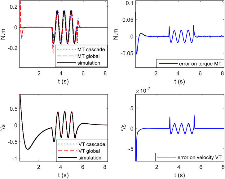
FIGURE 4. left: estimation of lumbar velocity and torque by cascade observer and global observer compared to simulation; right: estimation error.

Real-Time Experiments

The protocol in real-time experiments is similar to simulation context with human joint angles resulting from experimental manipulations. The experiments were carried out according to the agreement of “comité d’éthique pour la recherche du Centre de Recherche Interdisciplinaire en réhabilitation du Grand-Montréal (CRIR-1083-0515R).” Two subjects were treated with different profiles: a 32-year-old woman (weight: 55 kg, tall: 162 cm) having a SCI in vertebra T6 for 3 years and a 53-year-old man (weight: 100 kg, tall: 180 cm) suffering from a SCI in vertebra in T11 for 10 years.

The experimental protocol is as follows: the subject is asked to keep his seated balance while applying a disturbing force to the level of the T6 vertebra of the trunk. Once disturbed, each subject tries to stabilize himself by designing a compensatory strategy using the upper limbs. Figure 5 gives the estimated real-time lumbar couple of the global 2D-S3S observer and the cascade local observer as well as the difference. Results of the real-time experiments confirm the simulation results and show the similarity between the response of the global observer and the cascade observer. The difference in behaviors after applying the disturbing force depends on the level of the injury and its severity. Each subject in order to recover a stable behavior, has his/her own stabilization strategy based on the upper body part.

FIGURE 5

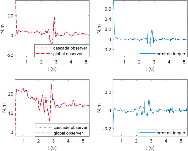
FIGURE 5. real-time lumbar torque estimated by cascade observer and global observer: top first subject and bottom second subject.

At last, note that the Trunk torque is positive at the beginning of each experimental acquisition, which makes sense from a mechanical balance point of view because the angle $q_0$ is negative at that time (a positive articular torque rotates the segment counterclockwise). Once the disturbing force applied, the joint torque decreases. This significant reduction is related to the disturbance which pushes each subject in the direction anterior to what is equivalent to injecting a negative torque (resp. positive) at the level of the trunk (resp. of the shoulder) (Blandeau, 2018).

Conclusion

People living with a SCI sitting position has been described via a so-called S3S model (Blandeau, 2018). The main goal is to be able to understand the different strategies that can be used by the people with the SCI. The internal control to stabilize the 2D-S3S model was out of the scope of this study and previously solved in Guerra et al. (2020). Understanding the strategies amounts to finding the torques that are unmeasured variables. A first PI-observer was derived in a discrete form in Blandeau (2018). In continuous, due to the problem of unmeasured variables in the premises of the quasi-LPV model, the problem was not solved. The first part of this study answered to this question especially thinking to push farther as possible the building of the polytope. The next step is to go to a more precise model especially including the sagittal plane, thus going to a 2D-S3S to its 3D-S3S form. Even if perfectly suitable for the 2D-S3S model, the global PI-observer solution ends with number of variables and LMI constraints that is very certainly not compatible for the 3D-S3S with actual solvers.

Therefore, two different solutions can apply. The first one consists in simplifying the model (partial linearization for example) but then introduces modeling errors in the observer. The second one, presented in this study, consists in using a cascade of observers. From an initial separation-like property, the 2D-S3S has been decomposed via two descriptors quasi-LPV observers, which design involved much more simplified LMI constraints problems.

Simulation and real-time experiments show that both approaches are suitable for the 2D-S3S model. Thus, not only the continuous global PI-observer design is validated but also the cascade observers using a decomposed form. Thus, it also validates the future steps to get a solution for a 3D-S3S model.

Thereby, as a final goal, we will be able to provide the occupational therapist with real time torques during rehabilitation exercises in order to follow the learning of new stabilization strategies outside the sagittal plan.

Data Availability Statement

The original contributions presented in the study are included in the article/Supplementary Material; further inquiries can be directed to the corresponding author.

Ethics Statement

The studies involving human participants were reviewed and approved by comité d’éthique pour la recherche du Centre de Recherche Interdisciplinaire en réhabilitation du Grand-Montréal (CRIR-1083-0515R). The patients/participants provided their written informed consent to participate in this study.

Author Contributions

All authors listed have made a substantial, direct, and intellectual contribution to the work and approved it for publication.

Funding

This work was partly supported by Zodiac Seats France and Direction Générale de l’Aviation Civile (project n°2014 930181). The present research work has been supported by the European Community, the French Ministry de l'Education Nationale, de la Recherche et de la Technologie, the Region Hauts-de-France, the Centre National de la Recherche Scientifique (CNRS); in part through the project ELSAT2020.

Conflict of Interest

The authors declare that the research was conducted in the absence of any commercial or financial relationships that could be construed as a potential conflict of interest.

Publisher’s Note

All claims expressed in this article are solely those of the authors and do not necessarily represent those of their affiliated organizations, or those of the publisher, the editors, and the reviewers. Any product that may be evaluated in this article, or claim that may be made by its manufacturer, is not guaranteed or endorsed by the publisher.

Acknowledgments

The authors gratefully acknowledge the support of these institutions.

Footnotes

¹ Blandeau, M., Guerra, T. M., Dequidt, A., Pudlo, P., and Gagnon, D. H. (2021). “A nonlinear biomechanical model for studying sitting control for people living with a spinal cord injury – IEEE T,” in Control Systems Technology. (under review).

References

Blandeau, M., Estrada-Manzo, V., Guerra, T. M., Pudlo, P., and Gabrielli, F. (2018). Fuzzy unknown input observer for understanding sitting control of persons living with spinal cord injury. Eng. Appl. Artif. Intelligence 67, 381–389. doi:10.1016/j.engappai.2017.09.016

CrossRef Full Text | Google Scholar

Blandeau, M. (2018). Modélisation Et Caractérisation De La Stabilité En Position Assise Chez Les Personnes Vivant Avec Une Lésion De La Moelle Épinière. PhD Thesis. Université de Valenciennes et du Hainaut-Cambresis. Valenciennes: Université Polytechnique Hauts-de-France.

Google Scholar

Bouarar, T., Guelton, K., and Manamanni, N. (2010). Robust fuzzy Lyapunov stabilization for uncertain and disturbed Takagi-Sugeno descriptors. ISA Trans. 49 (4), 447–461. doi:10.1016/j.isatra.2010.06.003

PubMed Abstract | CrossRef Full Text | Google Scholar

Boyd, S., Ghaoui, L. E., Feron, E., and Balakrishnan, V. (1994). Linear Matrix Inequalities in System and Control Theory. Pennsylvania: Society for Industrial and Applied Mathematics.

Google Scholar

Chadli, M., and Darouach, M. (2012). Novel bounded real lemma for discrete-time descriptor systems: Application to H∞ control design. Automatica 48 (2), 449–453. doi:10.1016/j.automatica.2011.10.003

CrossRef Full Text | Google Scholar

Chen, J., Patton, R. J., and Zhang, H.-Y. (1996). Design of unknown input observers and robust fault detection filters. Int. J. Control 63 (1), 85–105. doi:10.1080/00207179608921833

CrossRef Full Text | Google Scholar

Fang, Y., Morse, L. R., Nguyen, N., Tsantes, N. G., and Troy, K. L. (2017). Anthropometric and biomechanical characteristics of body segments in persons with spinal cord injury. J. Biomech. 55, 11–17. doi:10.1016/j.jbiomech.2017.01.036

PubMed Abstract | CrossRef Full Text | Google Scholar

Grip, H. F., Saberi, A., and Johansen, T. A. (2012). Observers for interconnected nonlinear and linear systems. Automatica 48 (7), 1339–1346. doi:10.1016/j.automatica.2012.04.008

CrossRef Full Text | Google Scholar

Guerra, T.-M., Bernal, M., and Blandeau, M. (2018). Reducing the Number of Vertices in Some Takagi-Sugeno Models: Example in the Mechanical Field. IFAC-PapersOnLine 51 (10), 133–138. doi:10.1016/j.ifacol.2018.06.250

CrossRef Full Text | Google Scholar

Guerra, T. M., Blandeau, M., Nguyen, A. T., Srihi, H., and Dequidt, A. (2020). “Stabilizing unstable biomechanical model to understand sitting stability for persons with spinal cord injury,” in IFAC- PapersOnLine (Berlin, Gemany: World Congress). doi:10.1016/j.ifacol.2020.12.2225

CrossRef Full Text | Google Scholar

Guerra, T. M., Estrada-Manzo, V., and Lendek, Z. (2015). Observer design for Takagi-Sugeno descriptor models: An LMI approach. Automatica 52, 154–159. doi:10.1016/j.automatica.2014.11.008

CrossRef Full Text | Google Scholar

Ichalal, D., and Guerra, T. M. (2019). Decoupling unknown input observer for nonlinear quasi-LPV systems. IEEE 58th Conf. Decis. Control. (Cdc), 3799–3804. doi:10.1109/cdc40024.2019.9029339

CrossRef Full Text | Google Scholar

Khalil, W., and Dombre, E. (2004). Google-Books-ID: nyrY0Pu5kl0C. Modeling, Identification and Control of Robots. UK: Butterworth-Heinemann.

Google Scholar

Lendek, Z., Nagy, Z., and Lauber, J. (2018). Local stabilization of discrete-time TS descriptor systems. Eng. Appl. Artif. Intelligence 67, 409–418. doi:10.1016/j.engappai.2017.09.006

CrossRef Full Text | Google Scholar

Lendek, Zs., Babuska, R., and De Schutter, B. (2008). Stability of cascaded fuzzy systems and observers. IEEE Trans. Fuzzy Syst. 17 (3), 641–653.

Google Scholar

Lendek, Zs., Guerra, T. M., Babuska, R., and De Schutter, B. (2010). Stability Analysis and nonlinear observer design using Takagi-Sugeno fuzzy models. Stud. fuzziness soft Comput. Vol. 262, 2010938248. Library of Congress Control Number.

Google Scholar

Potten, Y. J. M., Seelen, H. A. M., Drukker, J., Reulen, J. P. H., and Drost, M. R. (1999). Postural muscle responses in the spinal cord injured persons during forward reaching. Ergonomics 42, 1200–1215. doi:10.1080/001401399185081

PubMed Abstract | CrossRef Full Text | Google Scholar

Skelton, R. E., Iwasaki, T., and Grigoriadis, D. E. (1997). A Unified Algebraic Approach to Control Design. Routledge, 1997.

Google Scholar

Tanaka, K., and Wang, O. H. (2001). Fuzzy Control Systems Design and Analysis: A Linear Matrix Inequality Approach. New York: Wiley.

Google Scholar

Taniguchi, T., Tanaka, K., and Wang, H. O. (2000). Fuzzy descriptor systems and nonlinear model following control. IEEE Trans. Fuzzy Syst. 8 (4), 442–452. doi:10.1109/91.868950

CrossRef Full Text | Google Scholar

Varga, A. (1995). On stabilization methods of descriptor systems. Syst. Control. Lett., 1995. doi:10.1016/0167-6911(94)00017-p

CrossRef Full Text | Google Scholar

Zemouche, A., Boutayeb, M., and Bara, G. I. (2008). Observers for a class of Lipschitz systems with extension to performance analysis. Syst. Control. Lett. 57 (1), 18–27. doi:10.1016/j.sysconle.2007.06.012

CrossRef Full Text | Google Scholar