Quantification of Fractional Dynamical Stability of EEG Signals as a Bio-Marker for Cognitive Motor Control

1 Introduction

Systems biology and biomedicine has been studied in conjunction with control theory over several decades (Wiener, 2019). By applying the tools developed in control theory to biological and biomedical systems, new discoveries have been made that enhance our understanding of both the function and dysfunction of biological systems. One such control theoretic tool is stability, which has been particularly useful in uncovering new critical insights in a multitude of biological and biomedical applications (Wang and Zhang, 2009; Zhang et al., 2015; Li et al., 2017). Stability assesses the long-term behavior of a dynamical model and its equilibrium properties, which are critical to understanding the nature of the underlying biological or biomedical process and its characteristics. However, the accuracy of such conclusions drawn on the properties of the biological or biomedical process under observation will depend on the quality-of-fit of the model that is used to describe the underlying process. Assessing the goodness-of-fit requires measurements of the biological process.

There are many different tools to measure neurophysiological signals, including electrocardiogram (ECG), electromyogram (EMG), electroencephalogram (EEG), and blood oxygenation level dependent (BOLD), and their models have been studied in the literature (Baleanu et al., 2011; Magin, 2012; Pequito et al., 2015; Xue et al., 2016b; Gupta et al., 2018). In this paper, we restrict our attention to non-invasive scalp EEG, which has been widely used to draw conclusions on disease diagnosis, develop treatment, and gain a fundamental understanding of systems biology on the whole (Haddad et al., 2010; McFarland et al., 2010).

There is evidence that discrete-time linear fractional-order dynamical systems (DTLFOS) are well-suited to describe EEG signals and forecast their evolution (Pequito et al., 2015; Gupta et al., 2018). Furthermore, these nonlinear spatiotemporal models rely on only a few parameters (Caponetto, 2010; Xue et al., 2016b; Monje et al., 2010). These parameters include a coupling matrix and a set of temporal scale coefficients called fractional exponents. The coupling matrix describes the spatial dependencies between different state variables. The fractional exponents describe the long-term memory of the dynamical process across different state variables. With these few required and easy-to-interpret parameters, together with the superior goodness-of-fit, these DTLFOS models present distinct advantages over both linear time-invariant and (generically) nonlinear models. Specifically, LTI systems are limited in their ability to capture different time-scales occurring in biological applications, which are inherently modeled by the spatial component (i.e., the system’s autonomous matrix) (Pequito et al., 2015; Xue et al., 2016a; Xue and Bogdan, 2017). On the other hand, spatiotemporal nonlinear systems have been widely accepted as tools capable of accurately modeling EEG data but may lead to over-complicated and difficult to interpret models that often over-fit the data.

Despite the advantages of DTLFOS, there are few results regarding the stability of fractional-order systems (FOS). The prior literature describes conditions for continuous-time FOS (Benzaouia et al., 2014) and for single-input single-output continuous-time commensurate systems (i.e., systems with equal fractional exponents across state variables) (Dastjerdi et al., 2019). In Dzieliński and Sierociuk (2008), the authors leverage an infinite dimensional representation of truncated DTLFOS (i.e., with finite memory) to give conservative sufficient conditions for stability. While the work in (Busłowicz and Ruszewski, 2013) does provide necessary and sufficient conditions for practical and asymptotic stability of DTLFOS, they only consider commesurate-order systems (i.e., α is the same for all state variables). That said, a comprehensive analysis of DTLFOS stability is lacking.

Henceforth, we aim to analyze the quantification of stability of DTLFOS that encode EEG signals giving us the ability to unveil new insights on the relation between neural behavior and cognitive motor control. The prior literature describes methods using EEG signals to classify various movements with varying levels of success (Morash et al., 2008; Kim et al., 2019; Ofner et al., 2019). However, to the best of our knowledge, analyzing the stability of DTLFOS that model EEG signals to draw conclusions on cognitive motor control is a novel approach.

Subsequently, the main contributions of this work are as follows. First, we introduce stability conditions for multivariate DTLFOS with arbitrary fractional exponents. We then leverage these conditions to study the stability of a real-world EEG motor data set modeled as a DTLFOS and provide evidence of its relevance in the context of cognitive motor control.

2 Materials and Methods

2.1 Discrete-Time Linear Fractional-Order System

In this paper, we consider discrete-time linear fractional-order non-commensurate systems described by

${\mathrm{\Delta }}^{\alpha }x\left[k+1\right]=Ax\left[k\right],(1)$

where $x\in {\mathbb{R}}^n$ denotes the state and Δ^α is the Grünwald-Letnikov discretization of the fractional derivative. The Grünwald-Letnikov discretization for any i-th state (1 ≤ i ≤ n) can be expressed as ${\mathrm{\Delta }}^{{\alpha }_i}{x}_i[k]=\sum _{j=0}^k\psi ({\alpha }_i,j)x_i[k-j]$, where ${\alpha }_i\in \mathbb{R}$ is the fractional-order coefficient of the ith state and $\psi ({\alpha }_i,j)=\frac{\mathrm{\Gamma }(j-{\alpha }_i)}{\mathrm{\Gamma }(-{\alpha }_i)\mathrm{\Gamma }(j+1)}$ with Γ(⋅) denoting the Gamma function (Dzielinski and Sierociuk, 2005).

Notice that System (Eq. 1) is a (finite-dimensional) nonlinear (non-Markovian) system, and it considers a weighted linear combination of all the previous data from the beginning to the current time. As can be noticed from the Grünwald-Letnikov discretization formula, the magnitude of the fractional-order derivative necessitates the total number of previous data points and the weights on those data points. Intuitively, a larger fractional-order coefficient (i.e., α closer to 1) implies a lower dependency on the previous data meaning that the weights decay at a faster rate. Furthermore, as the fractional-order coefficient α approaches 1, the system becomes closer to an integer-order linear time-invariant system.

Towards deriving the stability conditions for DTLFOS, we start by noticing that the DTLFOS (Eq. 1) can be re-written as [Lemma 2, (Gupta et al., 2018)]:

$x\left[k\right]=G_{k}x\left[0\right],(2)$

where

$G_k=\left\{\begin{array}{cc}{I}_n,\hfill & k=0\hfill \\ \sum _{j=0}^{k-1}{A}_j{G}_{k-1-j},\hfill & k\ge 1\hfill \end{array}\right.(3)$

with A₀ = A − D(α, 1), A_j = − D(α, j + 1), for j ≥ 1, and

$D\left(\alpha ,j\right)=\left[\begin{array}{cccc}\hfill \psi \left({\alpha }_1,j\right)\hfill & \hfill 0\hfill & \hfill \dots \hfill & \hfill 0\hfill \\ \hfill 0\hfill & \hfill \psi \left({\alpha }_2,j\right)\hfill & \hfill \dots \hfill & \hfill 0\hfill \\ \hfill 0\hfill & \hfill ⋮\hfill & \hfill \ddots \hfill & \hfill 0\hfill \\ \hfill 0\hfill & \hfill 0\hfill & \hfill \dots \hfill & \hfill \psi \left({\alpha }_n,j\right)\hfill \end{array}\right].(4)$

In particular, we observe that Eq. 2 will lead to the following realizations.

$\begin{array}{cc}\hfill G_0& =I_n\hfill \\ \hfill G_1& =A-D\left(\alpha ,1\right)\hfill \\ \hfill G_2& =A^2-AD\left(\alpha ,1\right)-D\left(\alpha ,1\right)A+D{\left(\alpha ,1\right)}^2-D\left(\alpha ,2\right)\hfill \\ \hfill G_3& =A^3-AD\left(\alpha ,1\right)-D\left(\alpha ,1\right)A^2+D{\left(\alpha ,1\right)}^2-A^{2}D\left(\alpha ,1\right)+AD{\left(\alpha ,1\right)}^2+D\left(\alpha ,1\right)AD\left(\alpha ,1\right)\hfill \\ \hfill & +D{\left(\alpha ,1\right)}^3-AD\left(\alpha ,2\right)+D\left(\alpha ,1\right)D\left(\alpha ,2\right)-D\left(\alpha ,2\right)A+D\left(\alpha ,2\right)D\left(\alpha ,1\right)-D\left(\alpha ,3\right)\hfill \\ ⋮\hfill \end{array}(5)$

Using Equation 2, we show that a DTLFOS as in Eq. 1 can be represented as a discrete-time linear time-varying (DTLTV) system under mild assumptions. First, we notice that a DTLTV is described by

$x\left[k+1\right]=M_{k}x\left[k\right],(6)$

with a state-transition matrix (that follows from using Eq. 6 recursively)

$x\left[k\right]=\left(\prod _{i=0}^{k-1}{M}_{k-1-i}\right)x\left[0\right],(7)$

which provides a mapping from the initial state to the state at any time k. Consequently, from Eqs 2, 7, we find the conditions for which a DTLFOS can be represented as a DTLTV by equating the state-transition matrices $G_k=\prod _{i=0}^{k-1}{M}_{k-1-i},\forall k$.

Next, we observe that $M_k=G_{k+1}{G}_k^{-1}$ under the assumption that G_k is invertible for all k. In particular, we notice that $\prod _{i=0}^{k-1}{M}_{k-1-i}=\prod _{i=0}^{k-1}{G}_{k-i}{G}_{k-1-i}^{-1}=(G_k{G}_{k-1}^{-1})(G_{k-1}{G}_{k-2}^{-1})(G_{k-2}{G}_{k-3}^{-1})\dots ,G_1{G}_0^{-1}=G_k{G}_0^{-1}=G_k$.

Notice that the assumption on the invertability of G_k for all k can be seen as a mild assumption by invoking measure theoretical arguments. Simply speaking, consider any random matrix A, which is invertible almost surely since having a non-invertible A would require the determinant of A to be zero, which has a zero probability of occurring. From Eq. 5, we see that there would need to be a very specific combination to make G_k have a determinant of zero and thus be non-invertible, which again occurs with probability zero. Since the specific combinations required to make G_k have a zero determinant are different for each k, we do not define the specific combination; however, we can give some intuition as to what this combination might be by providing some examples. We remark that for G₁, the diagonal entries of D (α, 1) would need to be such that when subtracted from A, the matrix A − D (α, 1) is not invertible. Similarly for G₃, we see that there needs to be specific combinations of the matrices A, D (α, 1), D (α, 2), D (α, 3) and any certain powers of these to attain a non-invertible matrix G₃. From these examples, we see that the specific combination for a matrix G_k to be non-invertible is dependent on A, D (α, i), and any powers of these up to i, where i = {1,…, k}.

By showing that the DTLFOS can be re-cast as a DTLTV system under certain assumptions, we can now leverage the stability results from DTLTV systems to derive a stability condition for DTLFOS.

We start by introducing the definition of stability.

Theoretical Stability: (Section 4.1, (Khalil, 2014)) A DTLFOS system (Eq. 1) where G_k is invertible for all k system is said to be

• stable if for any ϵ > 0 and for any k₀, there exists a δ(k₀, ϵ) > 0 such that ‖x [k₀]‖₂ ≤ δ(k₀, ϵ) ⇒ ‖x [k]‖₂ ≤ ϵ, ∀k ≥ k₀.

• unstable if it is not stable.

In the main result, we provide the necessary and sufficient conditions of stability for DTLFOS (1).

Theorem 1. A DTLFOS (1), where G_k is invertible for all $k\in \mathbb{N}$, is stable if and only if there exists some constant 0 < c(k₀) < ∞ such that

$\Vert G_k{G}_{k-1}^{-1}{\Vert }_2\le c\left(k_0\right),\forall k,k_0,(8)$

where k ≥ k₀.

PROOF. Assuming that G_k is invertible for all $k\in \mathbb{N}$, it follows that we can represent the DTLFOS as a LTV system, i.e., x[k + 1] = M_kx[k], where $M_k=G_{k+1}{G}_k^{-1}$. Leveraging the fact that the DTLFOS can be represented as a LTV, we know that a discrete-time LTV system is stable if and only if for any k₀, there exists a 0 < γ(k₀) < ∞, such that ‖Φ(k, k₀)‖₂ ≤ γ(k₀), ∀k, k₀, where k ≥ k₀ and Φ(k, k₀) is the state-transition matrix from the state at k₀ to the state at k [Lemma 1, (Zhou and Zhao, 2017)]. Therefore, to show sufficiency, we notice that

$\begin{array}{cc}\hfill \Vert \mathrm{\Phi }\left(k,k_0\right){\Vert }_2& =\Vert M_{k-1}\dots ,M_{k_0}{\Vert }_2\hfill \\ \hfill & \le \Vert G_k{G}_{k-1}^{-1}{\Vert }_2\Vert G_{k-1}{G}_{k-2}^{-1}{\Vert }_2\dots \Vert G_{k_0+1}{G}_{k_0}^{-1}{\Vert }_2\hfill \\ \hfill & \le c{\left(k_0\right)}^{k-k_0}=\gamma \left(k_0\right).\hfill \end{array}$

The necessary condition can be shown by contradiction. Suppose that there exists an index k_i for which there does not exist a 0 < c (k₀) < ∞ such that $\Vert G_{k_i}{G}_{k_i-1}^{-1}{\Vert }_2\le c(k_0)$, then it must mean that $\Vert G_{k_i}{G}_{k_i-1}^{-1}{\Vert }_2>\infty$, so ‖Φ(k_i, k₀)‖₂ > ∞, so the system is unstable.We define the quantification of stability at time k in the following definition.

Definition 1. The quantification of stability at time k is defined by the magnitude of the stability metric $\Vert G_k{G}_{k-1}^{-1}{\Vert }_2$ given that $\Vert G_k{G}_{k-1}^{-1}{\Vert }_2<\infty$.Given EEG signals during a period when a subject is resting and when s/he is performing task, we will fit these signals to two distinct DTLFOS for the rest and task periods by using the method outline in Xue et al. (2016b), which finds the parameters using least-squares regression. By comparing the stability and quantifying the stability metric $\Vert G_k{G}_{k-1}^{-1}{\Vert }_2$ of these two systems, we expect to observe differences that not only help distinguish these two activities but also aid in establishing and verifying new and existing conclusions in cognitive motor control.

3 Assessing the Quantification of Stability of EEG Signals as a Bio-Marker for Cognitive Motor Control

In this section, we leverage the stability of DTLFOS systems (Eq. 1) to assess EEG signals for motor movement. DTLFOS systems are stable if and only if $\Vert G_k{G}_{k-1}^{-1}{\Vert }_2$, is bounded by a finite constant for all time steps k.

We explore the stability of EEG signals in the motor cortex for 106 subjects completing simple motor tasks. In each trial, a target appears on the left side of a screen, at which point the subject opens and closes the left fist until the target disappears, then the subject relaxes (Schalk et al., 2004). This data set consists of over 1,500 trials corresponding to one- and 2-min EEG recordings, obtained from 106 volunteers (Goldberger et al., 2000).

We use the data collected from the six sensors over-top the motor cortex to fit two distinct DTLFOS (Xue et al., 2016b), one corresponding to when the subject is resting and the other corresponding to when the subject is completing the motor task. For each subject, we chose a one second window of time at which point the subject is resting and a subsequent one second window when the subject begins to perform the task (open and close the left fist). Using these two windows of data, we fit two DTLFOS, one corresponding to the resting period and the other corresponding to the movement task. With these two systems, we use Algorithm 1 to evaluate the stability of the DTLFOS for 160 time-steps. We note that if the stability metric, namely $\Vert G_k{G}_{k-1}^{-1}{\Vert }_2$ exceeded a threshold of 300, we replaced it with the value 300. We note that for the selected time windows all of the values of $\Vert G_k{G}_{k-1}^{-1}{\Vert }_2$ were less than infinity, so all systems were found to be stable. The time window should be selected carefully to avoid numerical instability (Xue et al., 2016b).

ALGORITHM 1

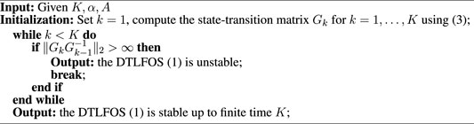
Algorithm 1. This algorithm is used to assess the stability of the DTLFOS (1) for a finite time horizon.

Briefly, we note that in general, these systems are stable. The stability metric $\Vert G_k{G}_{k-1}^{-1}\Vert$ captures the overall activity of the motor cortex. More specifically, $\Vert G_k{G}_{k-1}^{-1}\Vert$ over time captures the qualitative change of behavior of the underlying system as seen in the transient of the stability metric for Subjects 1, 2, and 3. We notice that during the task, the system has larger $\Vert G_k{G}_{k-1}^{-1}{\Vert }_2$ values when compared to the resting system. Previous work has shown that the neural activity in the motor cortex increases as muscles contract to perform a task (Chapter 37, Kandel et al. (2000)). This might explain why the task DTLFOS has higher $\Vert G_k{G}_{k-1}^{-1}{\Vert }_2$ values when compared to the resting DTLFOS since the higher brain activity while performing a task might be associated with an increase in $\Vert G_k{G}_{k-1}^{-1}{\Vert }_2$. Therefore, by observing that the stability metric quantitatively changed when comparing the rest system to the task system, this suggests that the behavior of the underlying system also changes. The larger $\Vert G_k{G}_{k-1}^{-1}{\Vert }_2$ values for the task system indicate that the quantification of the stability of DTLFOS can serve as a bio-marker for the brain’s change in behavior when switching from resting to movement tasks. We provide evidence to support this claim both by exploring several subjects and by statistically analyzing all 106 subjects through a Kolmogorov-Smirnov test (Hogg et al., 2010). The results for Subjects 1, 2, and 3 are presented in Figures 1, 3, 5, respectively. Furthermore, we evaluate the quality of fit by performing a one-step prediction for the rest and task DTLFOS and their corresponding Q-Q plots for Subjects 1, 2, and 3 in Figures 2, 4, 6, respectively.

FIGURE 1

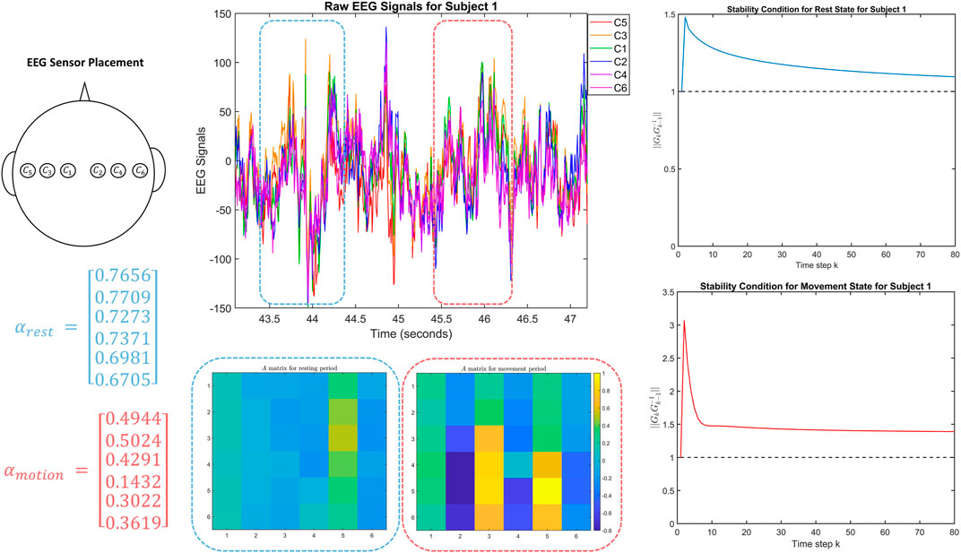
FIGURE 1. The top left figure shows the location of the EEG sensors on Subject 1 in the dataset. The top middle figure shows the corresponding EEG signals, including the one second windows used to model the two DTLFOS that correspond to rest (in blue) and task (in red). The bottom middle figures depict the two autonomous A matrices for the two DTLFOS representing resting state and task. The rows and columns correspond to the sensor scheme, where odd numbered sensors are on the left and even on the right. On the left are the fractional exponents (α) for the two DTLFOS representing resting state and task. Finally, on the right, the figures show the stability analysis for the two systems representing resting (top) and task (bottom).

FIGURE 2

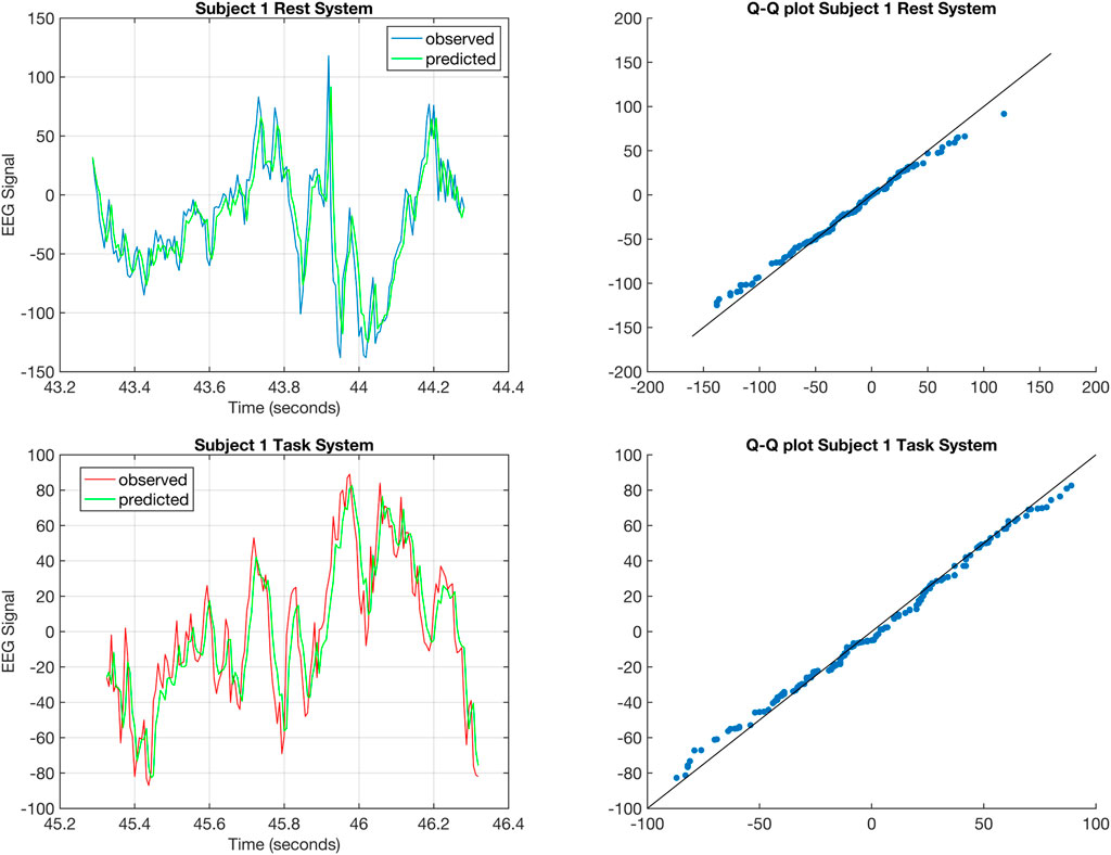
FIGURE 2. The top left figure shows the one-step prediction (Gupta et al., 2019) for the EEG signal from C₅ of Subject 1 corresponding to rest for a 1 s time window. The top right figure shows the Q-Q plot for the distributions of the predicted and observed EEG signal corresponding to rest for Subject 1. The bottom right figure shows the one-step prediction for the EEG signal from C₅ of Subject 1 corresponding to task for a 1 s time window. The bottom right figure shows the Q-Q plot for the distributions of the predicted and observed EEG signal corresponding to task for Subject 1.

In Figure 1, we observe several yellow squares appearing in the autonomous A matrix during the task. This is synonymous with the right side of the brain being activated during the movement of the left fist, which matches the conclusions of movement drawn by neuroscientists. These conclusions state that the right side of the brain controls the left side of the body and vice versa. Also during the task, we notice that the fractional exponents (α) are closer to 0.5 indicating that the system depends more heavily on information from signals in the very distant past. Therefore, a higher weight is being placed on previous states in the task system. However, in the resting system, the fractional exponents are closer to 1 indicating that the system does not depend on signals in the very distant past and requires less dependence on the previous states. The fact that the rest system does not depend heavily on previous states may be due to a possible transition between different cognitive states as expected in default mode (Breakspear, 2017).

In Figure 2, we evaluate the quality of fit by performing a one-step prediction for the rest and task DTLFOS and their corresponding Q-Q plots for Subject 1. The Q-Q plots shows that the fit is good when the points exhibit a linear relationship (Hogg et al., 2010). Figure 2 provides evidence that the estimated DTLFOS is a good fit for the EEG signals.

In the stability metric plots on the right side of Figure 1, the rest system and task system tend towards stability as the time-step increases, which is likely due to the fact that we are modeling an excited system driven by the inputs. As such, the behavior appearing in the stability analysis is similar to what would happen when applying an impulse or step input to a system, where we notice an initial transient followed by a return to stability.

We notice in the rest system that the value of $\Vert G_k{G}_{k-1}^{-1}{\Vert }_2$ peaks around 1.5, whereas in the task system the value of $\Vert G_k{G}_{k-1}^{-1}{\Vert }_2$ peaks around 3. In general the values of $\Vert G_k{G}_{k-1}^{-1}{\Vert }_2$ are larger for the task system than the rest system. Hence, we conclude that the quantification of stability of DTLFOS can help in providing further intuitions about the dynamics of the brain and serve as a bio-marker for its change in behavior.

In Figure 3, we see similar results to that of Subject 1, where during the task, the right side of the brain is activated and the fractional exponents are lower indicating that the task system depends heavily on previous states. We also see a similar behavior in the stability analysis where $\Vert G_k{G}_{k-1}^{-1}{\Vert }_2$ is larger during the task and reaches a peak around 2.2, whereas in the rest system, the peak is around 1.8.

FIGURE 3

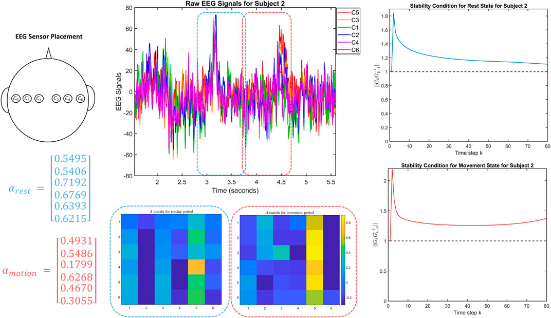
FIGURE 3. The top left figure shows the location of the EEG sensors on Subject 2 in the dataset. The top middle figure shows the corresponding EEG signals, including the one second windows used to fit the two DTLFOS that correspond to rest (in blue) and task (in red). The bottom middle figures depict the two autonomous A matrices for the two DTLFOS representing rest and task. The rows and columns correspond to the sensor scheme, where odd numbered sensors are on the left and even numbered sensors are on the right. On the left are the fractional exponents (α) for the two DTLFOS representing rest and task. Finally, on the right, the figures show the stability analysis for the two systems representing rest (top) and task (bottom).

While the Q-Q plots in Figure 4 do not exhibit a truly linear relationship, we argue that the results from Subject 2 still produce good results and so the fit of the estimated DTLFOS to the EEG signals is still fairly good.

FIGURE 4

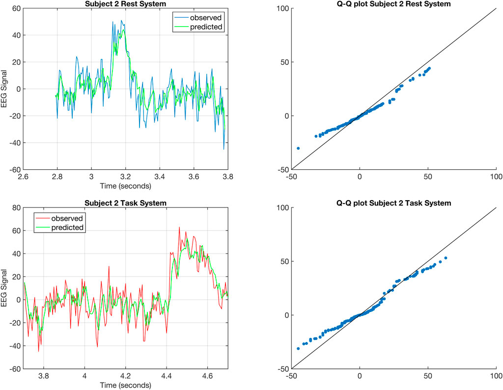
FIGURE 4. The top left figure shows the one-step prediction (Gupta et al., 2019) for the EEG signal from C₅ of Subject 2 corresponding to rest for a 1 s time window. The top right figure shows the Q-Q plot for the distributions of the predicted and observed EEG signal corresponding to rest for Subject 2. The bottom right figure shows the one-step prediction for the EEG signal from C₅ of Subject 2 corresponding to task for a 1 s time window. The bottom right figure shows the Q-Q plot for the distributions of the predicted and observed EEG signal corresponding to task for Subject 2.

Finally, in Figure 5 while despite being similar to that of Subjects 1 and 2, the results are less dramatic. However, we again note the same trends of the fractional exponents and the stability metrics for rest and task. In particular, the fractional-order exponents are lower for the task than for the rest system. Furthermore, the peak value for $\Vert G_k{G}_{k-1}^{-1}{\Vert }_2$ is around 1.4 for the task system and 1.1 for the rest system. The activation in the autonomous matrix is evident but much less pronounced and occurs in the middle of the motor cortex as opposed to on the presumed right side. Still, the results from Subject 3 support the fact that significant and important conclusions regarding motor movement, including the transition from rest to task, can be drawn from determining the quantification of stability of the EEG signals when fit as a DTLFOS. Furthermore, the quality of fit of the DTLFOS to the EEG signals is very good for Subject 3 as evidenced by the plots shown in Figure 6.

FIGURE 5

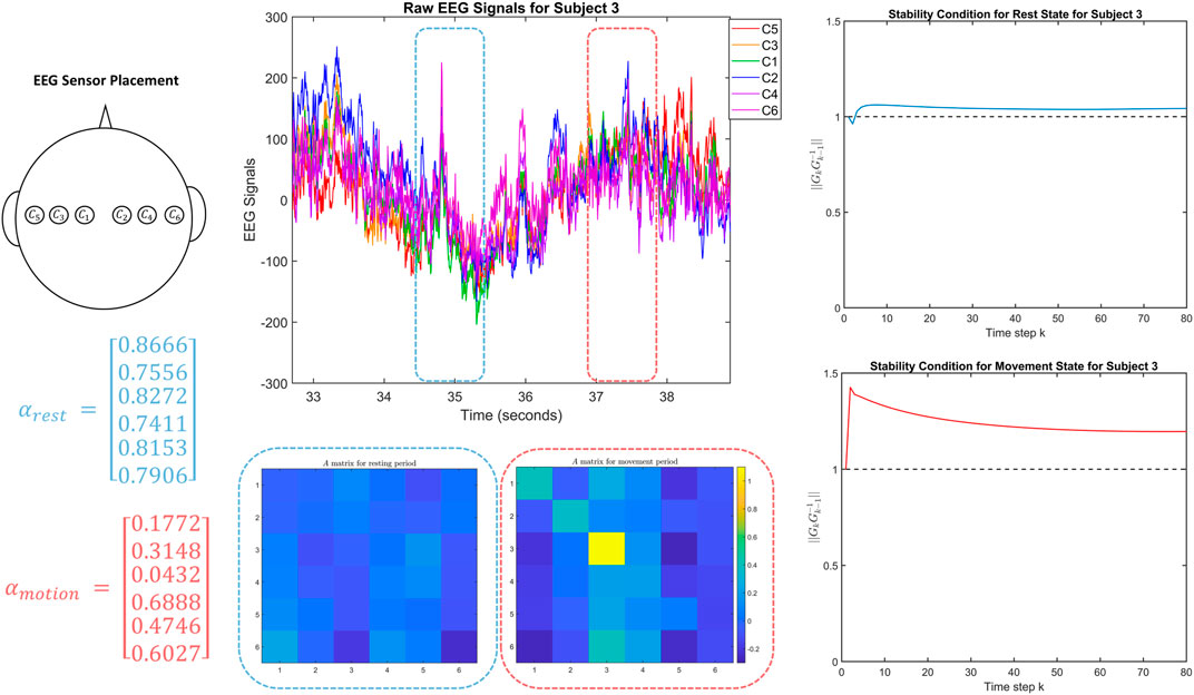
FIGURE 5. The top left figure shows the location of the EEG sensors on Subject 3 in the dataset. The top middle figure shows the corresponding EEG signals, including the one second windows used to fit the two DTLFOS that correspond to rest (in blue) and task (in red). The bottom middle figures depict the two autonomous A matrices for the two DTLFOS representing rest and task. The rows and columns correspond to the sensor scheme, where odd numbered sensors are on the left and even numbered sensors are on the right. On the left are the fractional exponents (α) for the two DTLFOS representing rest and task. Finally, on the right, the figures show the stability analysis for the two systems representing rest (top) and task (bottom).

FIGURE 6

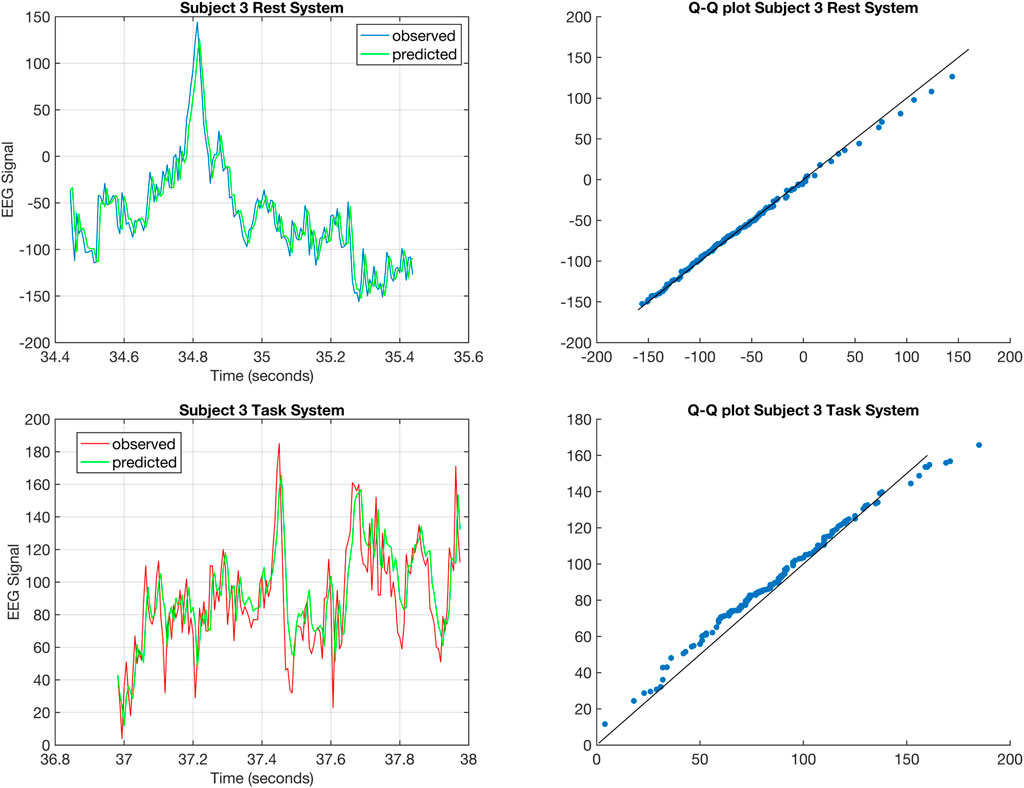
FIGURE 6. The top left figure shows the one-step prediction (Gupta et al., 2019) for the EEG signal from C₅ of Subject 3 corresponding to rest for a 1 s time window. The top right figure shows the Q-Q plot for the distributions of the predicted and observed EEG signal corresponding to rest for Subject 3. The bottom right figure shows the one-step prediction for the EEG signal from C₅ of Subject 3 corresponding to task for a 1 s time window. The bottom right figure shows the Q-Q plot for the distributions of the predicted and observed EEG signal corresponding to task for Subject 3.

Figure 7 show the average stability metric ($\Vert G_k{G}_{k-1}^{-1}{\Vert }_2$ for k = 1{1, … , 160}) across all 106 subjects during rest and task periods, respectively. It is important to point out that the average stability metric is larger during the task period than the rest period. Next, we provide statistical evidence that quantifying the average stability metric of EEG signals for rest and movement tasks indicates a change in the brain’s behavior and subsequently a bio-marker for cognitive motor control.

FIGURE 7

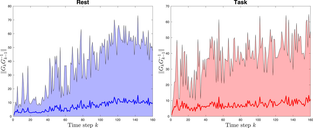
FIGURE 7. The left figure shows the average stability metric $\Vert G_k{G}_{k-1}^{-1}{\Vert }_2$ for the rest DTLFOS across all 106 subjects for time steps k = {1,…, 160}. The shaded region indicates the standard deviation and the solid blue line is the mean. The right figure shows the average stability metric $\Vert G_k{G}_{k-1}^{-1}{\Vert }_2$ for the task DTLFOS across all 106 subjects for time steps k = {1,…, 160}. The shaded region indicates the standard deviation and the solid red line is the mean.

We use the Kolmogorov-Smirnov test to show that indeed the distributions of the average values of the stability metric across 160 time steps ($\frac{1}{160}{\sum }_{k=1}^{160}\Vert G_k{G}_{k-1}^{-1}{\Vert }_2$ for the rest and task systems are significantly different. We start by finding the histogram plots of the average values of the stability metric across 160 time steps ($\frac{1}{160}{\sum }_{k=1}^{160}\Vert G_k{G}_{k-1}^{-1}{\Vert }_2$) for the rest and task systems for all 106 subjects in Figure 8. Next, we find the Kolmogorov-Smirnov statistic to be 0.0943. With an α level of 0.001, we find that the Kolmogorov-Smirnov statistic rejects the null hypothesis, meaning that the two distributions are statistically different. In particular, the rest distribution has more lower average values of the stability metric than the task distribution. This supports the conclusion found in Subjects 1-3 that the quantification of the stability of EEG signals modeled as a DTLFOS during rest and task are different, where the values of $\Vert G_k{G}_{k-1}^{-1}{\Vert }_2$ are generally larger for the task system when compared with the rest system.

FIGURE 8

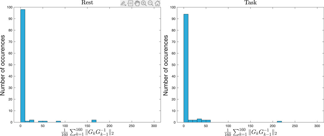
FIGURE 8. The left figure shows the histogram plot of the average stability metric $\frac{1}{160}{\sum }_{k=1}^{160}\Vert G_k{G}_{k-1}^{-1}{\Vert }_2$ for the rest DTLFOS for all 106 subjects. The right figure shows the histogram plot of the average stability metric $\frac{1}{160}{\sum }_{k=1}^{160}\Vert G_k{G}_{k-1}^{-1}{\Vert }_2$ for the task DTLFOS for all 106 subjects.

We find that the results hold for different window sizes. When considering a window size of 0.875 s, the Kolmogorov-Smirnov statistic is 0.0849, so the null hypothesis is rejected with an α level of 0.001. Similarly, when considering a window size of 1.25 s, the Kolmogorov-Smirnov statistic is 0.0755, so again the null hypothesis is rejected with an α level of 0.001. Hence, we provided evidence that the quantification of stability, namely how large the stability metric $\Vert G_k{G}_{k-1}^{-1}{\Vert }_2$ is compared to the baseline, can be used as a bio-marker for cognitive motor control, where the baseline is the subject at rest. This is significant because the quantification of stability can be used to design a discriminator for classifying EEG signals corresponding to rest or task.

In summary, this real-world example of fitting EEG signals to DTLFOS models and determining their quantification of stability leads to a deeper understanding of brain dynamics and motor movement.

4 Conclusions and Future Work

The quantification of stability plays a key role in unveiling important characteristics of biological systems. Notably, spatiotemporal discrete-time linear fractional-order systems can accurately and efficiently represent a variety of biological networks. We focused on physiological systems, especially EEG signals, and we leveraged the stability conditions for DTLFOS introduced in this paper to identify features that could serve as biomarkers for cognitive motor control. Specifically, we studied a real-world EEG data set consisting of 106 subjects and fit two different DTLFOS corresponding to the recordings during a subject’s rest and movement. We showed that analyzing the quantification of stability of these two systems is useful in distinguishing a change in the brain’s behavior, which can help enhance our understanding of motor movement and control.

In future work, we seek to determine necessary and sufficient conditions for stability of DTLFOS that are computationally tractable. In addition, we want to understand the trade-offs between the stability of the system and the memory captured by the system’s temporal parameters (fractional-order exponents), which will ultimately lead to a better understanding of how memory affects cognitive motor control and also neurological diseases (e.g., epilepsy).

Data Availability Statement

The original contributions presented in the study are included in the article/Supplementary Material, further inquiries can be directed to the corresponding author. The dataset analyzed for this study can be found in the https://physionet.org/content/eegmmidb/1.0.0/

Author Contributions

ER. derived the theoretical conditions and completed the experiments. PB. contributed to the development of the theoretical results and experiments, and revised the paper. SP. conceived the idea, contributed to the development of the theoretical results and experiments, and revised the paper.

Funding

ER. Reed acknowledges the support from the National Science Foundation through a Graduate Research Fellowship DGE-1842 487 and the University of Southern California through an Annenberg Fellowship and a WiSE Top-Off Fellowship. PB acknowledges the support by the National Science Foundation under the Career Award CPS/CNS-1453 860, the NSF awards under Grant numbers CCF-1837 131, MCB-1936 775, CNS-1932 620, and CMMI-1936 624, and the DARPA Young Faculty Award and DARPA Director Award under grant number N66001-17-1-4044. The views, opinions, and/or findings contained in this article are those of the authors and should not be interpreted as representing the official views or policies, either expressed or implied by the Defense Advanced Research Projects Agency, the Department of Defense or the National Science Foundation. SP acknowledges the support by the National Science Foundation under Grant number CMMI 1936 578.

Conflict of Interest

The authors declare that the research was conducted in the absence of any commercial or financial relationships that could be construed as a potential conflict of interest.

Publisher’s Note

All claims expressed in this article are solely those of the authors and do not necessarily represent those of their affiliated organizations, or those of the publisher, the editors and the reviewers. Any product that may be evaluated in this article, orclaim that may be made by its manufacturer, is not guaranteed or endorsed by the publisher.

Supplementary Material

The Supplementary Material for this article can be found online at: https://www.frontiersin.org/articles/10.3389/fcteg.2021.787747/full#supplementary-material

References

Baleanu, D., Machado, J. A. T., and Luo, A. C. (2011). Fractional Dynamics and Control. Berlin/Heidelberg, Germany: Springer Science & Business Media.

Google Scholar

Benzaouia, A., Hmamed, A., Mesquine, F., Benhayoun, M., and Tadeo, F. (2014). Stabilization of Continuous-Time Fractional Positive Systems by Using a Lyapunov Function. IEEE Trans. Automat. Contr. 59, 2203–2208. doi:10.1109/tac.2014.2303231

CrossRef Full Text | Google Scholar

Breakspear, M. (2017). Dynamic Models of Large-Scale Brain Activity. Nat. Neurosci. 20, 340–352. doi:10.1038/nn.4497

PubMed Abstract | CrossRef Full Text | Google Scholar

Busłowicz, M., and Ruszewski, A. (2013). Necessary and Sufficient Conditions for Stability of Fractional Discrete-Time Linear State-Space Systems. Bull. Polish Acad. Sci. Tech. Sci. 61, 4.

Google Scholar

Caponetto, R. (2010). Fractional Order Systems: Modeling and Control Applications, Vol. 72. Singapore: World Scientific.

Google Scholar

Dastjerdi, A. A., Vinagre, B. M., Chen, Y., and HosseinNia, S. H. (2019). Linear Fractional Order Controllers; a Survey in the Frequency Domain. Annu. Rev. Control. 47, 51–70. doi:10.1016/j.arcontrol.2019.03.008

CrossRef Full Text | Google Scholar

Dzielinski, A., and Sierociuk, D. “Adaptive Feedback Control of Fractional Order Discrete State-Space Systems,” in Proceedings of the International Conference on Computational Intelligence for Modelling, Control and Automation and international conference on intelligent agents, web technologies and internet commerce (IEEE), Vienna, Austria, November 2005, 804–809.

Google Scholar

Dzieliński, A., and Sierociuk, D. (2008). Stability of Discrete Fractional Order State-Space Systems. J. Vibration Control. 14, 1543–1556. doi:10.1177/1077546307087431

CrossRef Full Text | Google Scholar

Goldberger, A. L., Amaral, L. A., Glass, L., Hausdorff, J. M., Ivanov, P. C., Mark, R. G., et al. (2000). PhysioBank, PhysioToolkit, and PhysioNet: Components of a New Research Resource for Complex Physiologic Signals. Circulation 101 (23), E215–E220. Available at: https://physionet.org/content/eegmmidb/1.0.0/. doi:10.1161/01.cir.101.23.e215 (accessed October 10, 2020).

PubMed Abstract | CrossRef Full Text | Google Scholar

Gupta, G., Pequito, S., and Bogdan, P. “Dealing with Unknown Unknowns: Identification and Selection of Minimal Sensing for Fractional Dynamics with Unknown Inputs,” in Proceedings of the 2018 Annual American Control Conference. 2018 Annual American Control Conference (ACC) (IEEE), Milwaukee, WI, USA, June 2018, 2814–2820.

Google Scholar

Gupta, G., Pequito, S., and Bogdan, P. “Learning Latent Fractional Dynamics with Unknown Unknowns,” in Proceedings of the 2019 American Control Conference (ACC) (IEEE), Philadelphia, PA, USA, July 2019, 217–222.

Google Scholar

Haddad, W. M., Volyanskyy, K. Y., Bailey, J. M., and Im, J. J. (2010). Neuroadaptive Output Feedback Control for Automated Anesthesia with Noisy Eeg Measurements. IEEE Trans. Control. Syst. Technol. 19, 311–326.

Google Scholar

Hogg, R. V., Tanis, E. A., and Zimmerman, D. L. (2010). Probability and Statistical Inference. Upper Saddle River, NJ, USA: Pearson/Prentice Hall.

Google Scholar

Kandel, E. R., Schwartz, J. H., Jessell, T. M., Siegelbaum, S., Hudspeth, A. J., and Mack, S. (2000). Principles of Neural Science, Vol. 4. New York: McGraw-Hill.

Google Scholar

Khalil, H. K. (2014). Nonlinear Control. Hudson, New York: Pearson Higher Education.

Google Scholar

Kim, H., Yoshimura, N., and Koike, Y. (2019). Classification of Movement Intention Using Independent Components of Premovement Eeg. Front. Hum. Neurosci. 13, 63. doi:10.3389/fnhum.2019.00063

PubMed Abstract | CrossRef Full Text | Google Scholar

Li, A., Inati, S., Zaghloul, K., and Sarma, S. “Fragility in Epileptic Networks: the Epileptogenic Zone,” in Proceedings of the 2017 American Control Conference (IEEE), Seattle, WA, USA, May 2017, 2817–2822.

Google Scholar

Magin, R. L. “Fractional Calculus in Bioengineering: A Tool to Model Complex Dynamics,” in Proceedings of the 13th International Carpathian Control Conference (ICCC) (IEEE), High Tatras, Slovakia, May 2012, 464–469.

Google Scholar

McFarland, D. J., Sarnacki, W. A., and Wolpaw, J. R. (2010). Electroencephalographic (Eeg) Control of Three-Dimensional Movement. J. Neural Eng. 7, 036007. doi:10.1088/1741-2560/7/3/036007

CrossRef Full Text | Google Scholar

Monje, C. A., Chen, Y., Vinagre, B. M., Xue, D., and Feliu-Batlle, V. (2010). Fractional-order Systems and Controls: Fundamentals and Applications. Berlin/Heidelberg, Germany: Springer Science & Business Media.

Google Scholar

Morash, V., Bai, O., Furlani, S., Lin, P., and Hallett, M. (2008). Classifying Eeg Signals Preceding Right Hand, Left Hand, Tongue, and Right Foot Movements and Motor Imageries. Clin. Neurophysiol. 119, 2570–2578. doi:10.1016/j.clinph.2008.08.013

PubMed Abstract | CrossRef Full Text | Google Scholar

Ofner, P., Schwarz, A., Pereira, J., Wyss, D., Wildburger, R., and Müller-Putz, G. R. (2019). Attempted Arm and Hand Movements Can Be Decoded from Low-Frequency Eeg from Persons with Spinal Cord Injury. Sci. Rep. 9, 1–15. doi:10.1038/s41598-019-43594-9

PubMed Abstract | CrossRef Full Text | Google Scholar

Pequito, S., Bogdan, P., and Pappas, G. J. (2015). “Minimum Number of Probes for Brain Dynamics Observability,” in Proceedings of the 2015 54th IEEE Conference on Decision and Control (CDC) (IEEE), December 2015 (Osaka, Japan, 306–311. doi:10.1109/CDC.2015.7402218

CrossRef Full Text | Google Scholar

Schalk, G., McFarland, D. J., Hinterberger, T., Birbaumer, N., and Wolpaw, J. R. (2004). Bci2000: a General-Purpose Brain-Computer Interface (Bci) System. IEEE Trans. Biomed. Eng. 51, 1034–1043. doi:10.1109/tbme.2004.827072

PubMed Abstract | CrossRef Full Text | Google Scholar

Wang, Z., and Zhang, H. (2009). Global Asymptotic Stability of Reaction-Diffusion Cohen-Grossberg Neural Networks with Continuously Distributed Delays. IEEE Trans. Neural Netw. 21, 39–49. doi:10.1109/TNN.2009.2033910

PubMed Abstract | CrossRef Full Text | Google Scholar

Wiener, N. (2019). Cybernetics or Control and Communication in the Animal and the Machine. Cambridge, Massachusetts: MIT press.

Google Scholar

Xue, Y., and Bogdan, P. “Constructing Compact Causal Mathematical Models for Complex Dynamics,” in Proceedings of the 8th International Conference on Cyber-Physical Systems. (Association for Computing Machinery), Pittsburgh, PA USA, April 2017, 97–107.

Google Scholar

Xue, Y., Pequito, S., Coelho, J. R., Bogdan, P., and Pappas, G. J. (2016a). “Minimum Number of Sensors to Ensure Observability of Physiological Systems: A Case Study,” in Proceedings of the 2016 54th Annual Allerton Conference on Communication, Control, and Computing (Allerton) (IEEE), Monticello, IL, USA, September 2016, 1181–1188.

CrossRef Full Text | Google Scholar

Xue, Y., Rodriguez, S., and Bogdan, P. (2016b). “A Spatio-Temporal Fractal Model for a CPS Approach to Brain-Machine-Body Interfaces,” in Proceedings of the 2016 2016 Design, Automation Test in Europe Conference Exhibition (IEEE), Dresden, Germany, March 2016, 642–647.

CrossRef Full Text | Google Scholar

Zhang, X., Wu, L., and Zou, J. (2015). Globally Asymptotic Stability Analysis for Genetic Regulatory Networks with Mixed Delays: an M-Matrix-Based Approach. IEEE/ACM Trans. Comput. Biol. Bioinform. 13, 135–147. doi:10.1109/TCBB.2015.2424432

PubMed Abstract | CrossRef Full Text | Google Scholar

Zhou, B., and Zhao, T. (2017). On Asymptotic Stability of Discrete-Time Linear Time-Varying Systems. IEEE Trans. Automat. Contr. 62, 4274–4281. doi:10.1109/tac.2017.2689499

CrossRef Full Text | Google Scholar