Broad Learning Aided Model Predictive Control With Application to Continuous Stirred Tank Heater

1 Introduction

Tracking control plays an important role in the modern industrial process and has drawn much attention both in academia and industry over these years (Yin et al., 2017). As an efficient feedforward control strategy, model predictive control (MPC) has shown its efficiency in the tracking control of multivariable systems with various constraints. Compared with other control strategies where the control law is calculated offline, the core idea of MPC is to calculate an optimal control sequence by solving a finite optimal control problem online (Mayne and Rawlings, 2001). MPC is proved to be easy for implementation and maintenance in practical industry (Hidalgo and Brosilow, 1990; Yin and Xiao, 2017). Due to these advantages, MPC has been successfully used in the tracking control of the hybrid energy storage system, modular multi-level converters, wind generation system and many other applications in recent literatures (Qin and Badgwell, 2003; Garcia-Torres et al., 2019; Guo et al., 2019; Kou et al., 2019).

Despite the successful applications of MPC, most predictive controllers rely heavily on the precision of the predictive model. For model-based MPC, the predictive model is usually generated using the first principle, i.e., the controlled auto-regressive intergraded moving average (CARIMA) model (Zhang et al., 2018). However, it is arduous to set up a precise model for modern industrial process based on the first principle due to the complicated mechanism. Some alternative predictive models, such as the time-domain model, are also hard to obtain in practice (Patwardhan et al., 1998). Fortunately, there exists a huge number of underutilized process data with the development of the measurement and storage technology. Motivated by this, the data-driven predictive controller design has attracted the interest of researchers in recent years.

To propose the data-driven predictive control strategy, multivariable statistical analysis (MSA) techniques are used to identify the predictive model based on the available process data. Partial least square (PLS) and its modified forms have been paid more attention to due to the low computation complexity (Gao et al., 2018). To extract the dynamic characteristics of the process, a dynamic PLS based predictive control is proposed based on the assumed autoregressive exogenous (ARX) model (Kaspar and Ray, 1993). Subspace identification techniques are also used to design the predictive controller, where the state space model can be directly identified based on the process data (Yi, 2016; Garg and Mhaskar, 2017; Meidanshahi et al., 2017; Zhou et al., 2017). However, most investigations on subspace identification mainly focus on the identification of linear systems (Wu et al., 2013; Li et al., 2020). To cope with nonlinear systems, the neural network (NN) is often applied for the predictive controller design due to its strong learning ability in nonlinear model regression.

Over the past several years, fruitful achievements have been reported regarding the combination of NN and MPC. A dynamic neural network based MPC (DNN-MPC) is proposed and demonstrated to show superior control performance than the mathematical model based MPC for the industrial baker’s yeast drying process (Yuzgec et al., 2008). A self-organizing recurrent neural network (RNN) aided nonlinear MPC is proposed (Han et al., 2016), where the control performance is evaluated through a wastewater treatment process. To improve the control performance for nonlinear process, the radial basis function neural network (RBF-NN) is applied to design the model predictive controller (Yu et al., 2011). Particularly, an adaptive splitting and merging RBF-NN based MPC has recently been successfully implemented in a zinc hydrometallurgy plant. However, these NN based MPC strategies often require much computation load, which limits its extension to the online implementation for real-time control performance.

In this paper, a random vector functional-link neural network (RVFLNN), i.e., the broad learning system (Chen and Liu, 2018), is incorporated into the predictive controller design. By using the incremental broad learning algorithm, the predictive model can be identified adaptively based on the online process data. In addition, a Jacobian matrix is used to approximate the predictive model to enhance the precision of the predictive model. The main contributions can be summarized as follows:

1) A data-driven predictive control strategy is proposed based on the broad learning algorithm with no prior knowledge of the system model;

2) The proposed data-driven predictive controller can be updated online based on the incremental broad learning algorithm while requiring little computation load;

3) The proposed broad learning aided MPC strategy is verified on the continuous stirred tank heater (CSTH) benchmark for temperature adjustment.

The rest of this paper is organized as follows. Section 2 introduces the basic knowledge of the model predictive control and the fundamental structure of the broad learning system. Section 3 discusses the incremental broad learning algorithm for new training data and proposes the incremental broad learning based MPC. Section 4 verifies the control performance of the proposed broad learning based MPC through the CSTH benchmark. Section 5 concludes this paper.

2 Preliminaries

2.1 Basic Knowledge of Model Predictive Control

Given a nonlinear process described as follows:

$y\left(t\right)=f\left(y\left(t-1\right),\dots ,y\left(t-n_y\right),u\left(t\right),\dots ,\right.(1)$

$\left.u\left(t-n_u\right)\right)+d\left(t\right)(2)$

where $y(t)\in {\mathcal{R}}^m$ is the output of the system, $u(t)\in {\mathcal{R}}^l$ is the output of the controller, n_u and n_y represent the order of the system.

The core idea of MPC is to optimize the following quadratic problem online

$\begin{array}{cc}\hfill \mathit{min}J=& \sum _{i=1}^{n_p}{\left(y_{sp}\left(k+i\right)-y\left(k+i\right)\right)}^{\text{T}}{\lambda }_1\left(y_{sp}\left(k+i\right)-\right.\hfill \\ \hfill & \left.y\left(k+i\right)\right)+\sum _{i=1}^{n_c}\mathrm{\Delta }u{\left(k+i\right)}^{\text{T}}{\lambda }_2\mathrm{\Delta }u\left(k+i\right),\hfill \end{array}(3)$

or equivalently,

$\mathit{min}\underset{\mathrm{\Delta }U}{J}=\Vert Y_{sp}-\widehat{Y}{\Vert }_{{\lambda }_1}^2+\Vert \mathrm{\Delta }U{\Vert }_{{\lambda }_2}^2,(4)$

$\begin{array}{cc}\hfill u_{\mathit{min}}\le & u\left(t+j\right)\le u_{\mathit{max}}\hfill \\ \hfill s.t.\mathrm{\Delta }{u}_{\mathit{min}}\le \mathrm{\Delta }& u\left(t+j\right)\le \mathrm{\Delta }{u}_{\mathit{max}}\hfill \\ \hfill y_{\mathit{min}}\le & y\left(t+j\right)\le y_{\mathit{max}},\hfill \end{array}(5)$

where Y_sp is the setpoint of the process, $\widehat{Y}$ is the prediction of the output and ΔU is the incremental value of the controller output to be calculated. λ₁ and λ₂ are two weights to make a trade-off between the tracking error and the cost of the control action.

2.2 Basic Knowledge of Broad Learning

As an improved neural network generated from the RVFLNN, broad learning has been proven to be an efficient algorithm for regression and classification, where it is important to extract the features from the training data. A random initialization of the features is always a popular way due to its easy computation. However, the feature extracted by random projection may suffer from unpredictability and needs guidance. To avoid this, a set of sparse features can be extracted from the training data using the sparse autoencoder (SAE) discussed in Gong et al. (2015). In this way, the alternating direction method of multipliers (ADMM) technique can be used to solve the lasso problem in the broad learning algorithm (Chen and Liu, 2018) to fine-tune the weight matrices. The details of the broad learning is given as below.

Assume that $U\in {\mathcal{R}}^{N\times l}$ and $Y\in {\mathcal{R}}^{N\times m}$ respectively denote the collected input and output data with N samples. The ith mapped feature $Z_i\in {\mathcal{R}}^{N\times \alpha }$ can then be calculated as

$Z_i=\varphi \left(U{W}_{ei}+{\beta }_{ei}\right),(6)$

where ϕ(⋅) denotes the projection function, $W_{ei}\in {\mathcal{R}}^{l\times \alpha }$ and ${\beta }_{ei}\in {\mathcal{R}}^{N\times \alpha }$ are two random matrices.

Denote Zⁿ ≡ [Z₁, Z₂, …, Z_n] as the concentration of the mapped feature. Zⁿ can then be used to generate the jth enhancement node $H_j\in {\mathcal{R}}^{N\times \gamma }$ as

$H_j=\zeta \left(Z^n{W}_{hj}+{\beta }_{hj}\right),(7)$

where ζ(⋅) denotes the projection function, $W_{hj}\in {\mathcal{R}}^{\alpha \times \gamma }$ and ${\beta }_{hj}\in {\mathcal{R}}^{N\times \gamma }$ are two random matrices.

Similarly, denote H^m ≡ [H₁, H₂, …, H_m] as the collection of the enhancement nodes. In this way, the global model can be represented as

$Y=\left[Z^n\mid H^m\right]W^m=A_n^m{W}^m.(8)$

where $A_n^m\in {\mathcal{R}}^{N\times (n\alpha +m\gamma )}$ denotes the input matrix and $W^m\in {\mathcal{R}}^{(n\alpha +m\gamma )\times p}$ denotes the weight matrix.

It is straightforward that W^m can be calculated as

$W^m={\left(A_n^m\right)}^{+}Y.(9)$

where (⋅)⁺ represents the moore-penrose pseudoinverse. To reduce the computation complexity, the broad learning algorithm makes use of the ridge regression theory proposed in Hoerl and Kennard (2000).

Assume that $A_n^m$ is of full column rank, we have

${\left(A_n^m\right)}^{+}=\underset{\lambda \to 0}{\mathit{lim}}{\left(\lambda I+{\left(A_n^m\right)}^{\text{T}}{A}_n^m\right)}^{-1}{\left(A_n^m\right)}^{\text{T}},(10)$

and consequently,

$W^m=\underset{\lambda \to 0}{\mathit{lim}}{\left(\lambda I+{\left(A_n^m\right)}^{\text{T}}{A}_n^m\right)}^{-1}{\left(A_n^m\right)}^{\text{T}}Y.(11)$

The functional-linked broad learning model is shown in Figure 1. More details on the broad learning can be referred to Chen and Liu (2018).

FIGURE 1

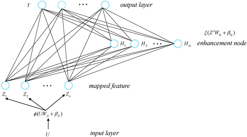
FIGURE 1. Functional-linked broad learning model.

3 Broad Learning Based Predictive Control

3.1 Incremental Broad Learning Algorithm

Though broad learning has been proven to be efficient for classification and regression, it is not easy to regress the process model based on the online data due to the unpredictable noise, model uncertainty and dynamic characteristics. To implement the predictive control in the framework of the broad learning, it is essential to develop the equivalent incremental broad learning algorithm. By updating the parameters of the broad learning model, the precision of the regression model can be further enhanced. The incremental broad learning algorithm for new training data was briefly discussed in Chen and Liu (2018). The details of the incremental broad learning for new training data will be presented in this section.

According to Chen and Wan (1999), the stepwise updating algorithm of a functional-linked neural network for a new enhancement node can be equivalently represented as adding several columns to the input matrix. Denote the initial input matrix as A_n, the final input matrix is then given as A_n+1 = [A_n|a] when a new enhancement node a is added to the neural network.

Inspired by the moore-penrose pseudo inverse of partitioned matrix mentioned in Diaz and Gutierrez (2006), the pseudo inverse of A_n+1 can be calculated as

$A_{n+1}=\left[\begin{array}{c}\hfill A_n^{+}-d{b}^{\top }\hfill \\ \hfill b^{\top }\hfill \end{array}\right],(12)$

where

$b^{\top }=\{\begin{array}{ccc}\hfill & c^{+}\hfill & \hfill ifc\ne 0\\ \hfill & {\left(1+d^{\top }d\right)}^{-1}{d}^{\top }{A}_n^{+}\hfill & \hfill ifc=0\end{array},(13)$

$d=A_n^{+}a,(14)$

$c=a-A_{n}d.(15)$

In this way, the new weights W_n+1 can be calculated as

$W_{n+1}=\left[\begin{array}{c}\hfill W_n-d{b}^{\top }{Y}_n\hfill \\ \hfill b^{\top }{Y}_n\hfill \end{array}\right],(16)$

Denote X_a and Y_a as a group of new training input data and the corresponding output data. The incremental algorithm broad learning for new training data can be demonstrated as Figure 2.

FIGURE 2

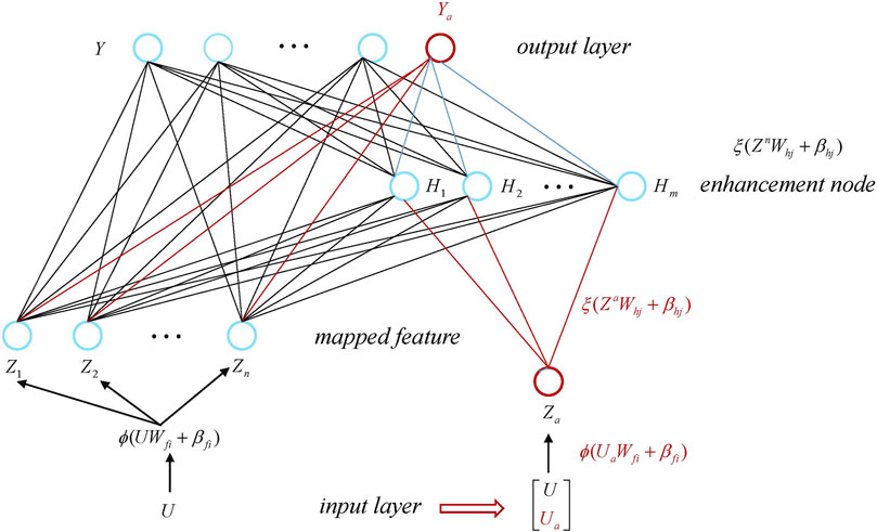
FIGURE 2. Incremental broad learning for new training data.

The original combination of feature nodes and enhancement nodes forms the following input matrix $A_n^m$:

$A_n^m=\left[\varphi \left(U{W}_{e1}+{\beta }_{e1}\right),\dots ,\varphi \left(U{W}_{en}+{\beta }_{en}\right)\mid \right.(17)$

$\left.\xi \left(Z^n{W}_{h1}+{\beta }_{h1}\right),\dots ,\xi \left(Z^n{W}_{hm}+{\beta }_{hm}\right)\right].(18)$

The input matrix ${}^{u}A_n^m$ trained by the new input data can be calculated as

$\begin{array}{ll}\hfill {}^{u}A_n^m=& [\varphi {(}^{a}U{W}_{e1}{+}^a{\beta }_{e1}),\dots ,\varphi {(}^{a}U{W}_{en}{+}^a{\beta }_{en})\mid \hfill \\ \hfill & \xi {(}^a{Z}^n{W}_{h1}{+}^a{\beta }_{h1}),\dots ,\xi {(}^a{Z}^n{W}_{hm}{+}^a{\beta }_{hm})],\hfill \end{array}(19)$

where

${}^{a}U=\left[\begin{array}{c}\hfill U\hfill \\ \hfill U_a\hfill \end{array}\right],{}^a\beta _{ei}=\left[\begin{array}{c}\hfill {\beta }_{ei}\hfill \\ \hfill {\beta }_{ei}^a\hfill \end{array}\right],i=1,\dots ,n,(20)$

${}^{a}Z^n=\left[\begin{array}{c}\hfill Z^n\hfill \\ \hfill Z^a\hfill \end{array}\right],{}^a\beta _{hi}=\left[\begin{array}{c}\hfill {\beta }_{hi}\hfill \\ \hfill {\beta }_{hi}^a\hfill \end{array}\right],i=1,\dots ,m,(21)$

$Z^a=\left[\varphi \left(U_a{W}_{e1}+{\beta }_{e1}^a\right),\dots ,\varphi \left(U_a{W}_{en}+{\beta }_{en}^a\right)\right).(22)$

It is obvious that ${}^{u}A_n^m$ can be equivalently constructed as adding several rows generated by U_a to the bottom of $A_n^m$.

Denote the input matrix generated by the new training data U_a as A_u, ${}^{u}A_n^m$ can then be represented as

${}^{u}A_n^m=\left[\begin{array}{c}\hfill A_n^m\hfill \\ \hfill A_u\hfill \end{array}\right],(23)$

where

$\begin{array}{ll}\hfill A_u=& \left[\varphi \left(U_a{W}_{e1}+{\beta }_{e1}^a\right),\dots ,\varphi \left(U_a{W}_{en}+{\beta }_{en}^a\right)\mid \right.\hfill \\ \hfill & \left.\xi \left(Z^a{W}_{h1}+{\beta }_{h1}^a\right),\dots ,\xi \left(Z^a{W}_{hm}+{\beta }_{hm}^a\right)\right].\hfill \end{array}(24)$

The pseudoinverse of ${}^{u}A_n^m$ can be calculated as

$\begin{array}{cc}\hfill {(}^u{A}_n^m{)}^{+}& ={\left({\left[{\left(A_n^m\right)}^{\top }\mid A_u^{\top }\right]}^{+}\right)}^{\top }\hfill \\ \hfill & ={\left[\begin{array}{c}\hfill {\left({\left(A_n^m\right)}^{+}\right)}^{\top }-D{B}^{\top }\hfill \\ \hfill B^{\top }\hfill \end{array}\right]}^{\top }\hfill \\ \hfill & =\left[{\left(A_n^m\right)}^{+}-B{D}^{\top }\mid B\right],\hfill \end{array}(25)$

where

$B=\left\{\begin{array}{ccc}\hfill & {\left(C^{\top }\right)}^{+}\hfill & \hfill ifC\ne 0\\ \hfill & {\left(A_n^m\right)}^{+}D{\left(1+D^{\top }D\right)}^{-1}\hfill & \hfill ifC=0\end{array}\right.,(26)$

$D^{\top }=A_u{\left(A_n^m\right)}^{+},(27)$

$C^{\top }=A_u-D^{\top }{A}_n^m.(28)$

The weight matrix of the new broad learning model can be calculated as

$\begin{array}{cc}\hfill {}^{u}W_n^m& =\left[{\left(A_n^m\right)}^{+}-B{D}^{\top }\mid B\right]\left[\begin{array}{c}\hfill Y\hfill \\ \hfill Y_a\hfill \end{array}\right]\hfill \\ \hfill & ={\left(A_n^m\right)}^{+}Y-B{D}^{\top }Y+B{Y}_a\hfill \\ \hfill & =W_n^m+B\left(Y_a-A_u{W}_n^m\right),\hfill \end{array}(29)$

The incremental broad learning algorithm for new training data can be summarized in Algorithm 1.

Remark 1. In fact, the broad learning algorithm is herein used to the establish the predictive model for control purpose. Note that the predictive model does not need to be retrained when the new data arrives if the incremental broad learning algorithm is applied. The main computation is spent on the update of the new weights ($i.e.,{}^{u}W_n^m$) and the pseudo inverse of input matrix ($i.e.,{}^{u}A_n^m$) based on the previous value when the predictive model needs to be updated, which requires less computational load compared with the basic broad learning algorithm (i.e., requires retraining the network model with full data)

3.2 Incremental Broad Learning Based Predictive Control

For predictive control purpose, the cost function J(k) to be minimized at the k^th instant can be given as follows,

$J\left(k\right)=\Vert Y_{sp}\left(k+1\right)-Y\left(k+1|k\right){\Vert }_{{\lambda }_1}^2+\Vert \mathrm{\Delta }U\left(k+1\right){\Vert }_{{\lambda }_2}^2,(30)$

where

$Y_{sp}\left(k+1\right)=\left[\begin{array}{c}\hfill y_{sp}\left(k+1\right)\hfill \\ \hfill y_{sp}\left(k+2\right)\hfill \\ \hfill ⋮\hfill \\ \hfill y_{sp}\left(k+n_p\right)\hfill \end{array}\right]\in {\mathcal{R}}^{\left(n_y\times n_p\right)\times 1},(31)$

$Y\left(k+1|k\right)=\left[\begin{array}{c}\hfill y\left(k+1|k\right)\hfill \\ \hfill y\left(k+2|k\right)\hfill \\ \hfill ⋮\hfill \\ \hfill y\left(k+n_c|k\right)\hfill \end{array}\right]\in {\mathcal{R}}^{\left(n_y\times n_c\right)\times 1},(32)$

$\mathrm{\Delta }U\left(k+1\right)=\left[\begin{array}{c}\hfill \mathrm{\Delta }u\left(k+1\right)\hfill \\ \hfill \mathrm{\Delta }u\left(k+2\right)\hfill \\ \hfill ⋮\hfill \\ \hfill \mathrm{\Delta }u\left(k+n_c\right)\hfill \end{array}\right]\in {\mathcal{R}}^{\left(n_u\times n_c\right)\times 1},(33)$

$\mathrm{\Delta }u\left(k+i\right)=u\left(k+i\right)-u\left(k\right).(34)$

and n_y, n_u, n_p, and n_c are the dimension of an output vector, the dimension of the input vector, the predictive horizon and the control horizon, respectively.

Remark 2. It is worth mentioning that n_p should be set to be longer than the settling time in order to satisfy the convergence condition of the predictive control (Rossiter, 2003). n_p has no influence on the convergence of predictive control if n_p is greater than the settling time. However, n_p is often determined based on the practical experience since the settling time is unknown. In this paper, the length of the control horizon n_c and prediction horizon n_p are both set to be 50.In the broad learning algorithm, the relationship between input training data U and output training data Y can be represented as

$Y=U{W}_0+{\beta }_0,(35)$

where

$W_0=\left[W_e,W_e{W}_h\right]W^m,(36)$

$W_e=\left[W_{e1},\dots ,W_{en}\right],W_h=\left[W_{h1},\dots ,W_{hn}\right],(37)$

${\beta }_0=\left[{\beta }_e,{\beta }_e{W}_h+{\beta }_h\right]W^m,(38)$

${\beta }_e=\left[{\beta }_{e1},\dots ,{\beta }_{en}\right],{\beta }_h=\left[{\beta }_{h1},\dots ,{\beta }_{hn}\right].(39)$

Therefore, regardless of the activation function, the correlation between u(k) and y(k) can be presented as

$y\left(k\right)={\left(W^m\right)}^{\text{T}}\left[\begin{array}{c}\hfill W_e^{\text{T}}u\left(k\right)\hfill \\ \hfill W_h^{\text{T}}{W}_e^{\text{T}}u\left(k\right)\hfill \end{array}\right],(40)$

However, the activation function F(⋅) is necessary to extract the nonlinear characteristics. In the broad learning, the prediction of y(k) is calculated as

$\begin{array}{cc}\hfill \widehat{y}\left(k\right)& ={\left(W^m\right)}^{\text{T}}\left[\begin{array}{c}\hfill W_e^{\text{T}}u\left(k\right)\hfill \\ \hfill F\left(Wu\left(k\right)\right)\hfill \end{array}\right]\hfill \\ \hfill & ={\left(W^m\right)}^{\text{T}}\left[\begin{array}{c}\hfill W_e^{\text{T}}u\left(k\right)\hfill \\ \hfill f\left(w_{\mathrm{1,1}}{u}_1+\cdots +w_{1,n_u}{u}_{n_u}\right)\hfill \\ \hfill ⋮\hfill \\ \hfill f\left(w_{h,1}{u}_1+\cdots +w_{h,n_u}{u}_{n_u}\right)\hfill \end{array}\right]\hfill \\ \hfill & ={\left(W^m\right)}^{\text{T}}\left[\begin{array}{c}\hfill W_e^{\text{T}}u\left(k\right)\hfill \\ \hfill f_1\left(u\right)\hfill \\ \hfill ⋮\hfill \\ \hfill f_h\left(u\right)\hfill \end{array}\right],\hfill \end{array}(41)$

where

$f\left(net\right)=\frac{1-e^{net}}{1+e^{net}}.(42)$

Note that the nonlinearity brings challenges to the receding optimization of the predictive control since the cost function to be minimized is nonlinear. Therefore, an appropriate approximation of the predictive model is necessary.According to Eq. 41, the prediction at the instant k can be rewritten as

$\widehat{y}\left(k\right)=G\left(u\left(k\right)\right),(43)$

Assume that u(k) is known, G(u(k)) can then be calculated easily via the general inverse. However, the incremental ΔU is to be calculated by solving the quadratic problem as Eq. 30. Take the prediction of the y(k + 1) at the instant k as an example,

$\begin{array}{cc}\hfill \widehat{y}\left(k+1\right)& =G\left(u\left(k+1\right)\right)\hfill \\ \hfill & =G\left(u\left(k\right)+\mathrm{\Delta }u\left(k+1\right)\right),\hfill \end{array}(44)$

where Δu(k + 1) is unknown.Since G(u) is continuous differentiable at any u, define the Jacobian matrix of G(u) as

$J_G\left(u\right)=G\prime \left(u\right),G\prime {\left(u\right)}_{ij}=\frac{\partial G_i}{\partial u_j}\left(u\right),(45)$

In this way, the approximation of G(u(k + 1)) can be given as

$\widehat{G}\left(u\left(k+1\right)\right)=G\left(u\left(k\right)\right)+J_G\left(u\left(k\right)\right)\mathrm{\Delta }u\left(k+1\right).(46)$

According to the definition of G(⋅) and f(net) as presented in Eqs 41, 42. It holds that f′(net) = 1 − f(net)² ≤ 1 and G(u) is continuously differentiable for any $u\in {\mathcal{R}}^{n_u}$. The Jacobian matrix J_G(u) is Lipschitz continuous for $u\in {\mathcal{R}}^{n_u}$. Therefore, there exists a Lipschitz constant γ such that for any $v\in {\mathcal{R}}^{n_u}$

$\Vert J_G\left(v\right)-J_G\left(u\right)\Vert \le \gamma \Vert v-u\Vert .(47)$

Theorem 1. Let Eqs 41, 42, 47 holds, replacing G(u(k)) with $\widehat{G}(u(k))$ has no influence on the convergence of the quadratic problem as shown in Eq. 30.

Proof. Define the deviation E_G between $\widehat{G}(u(k+1))$ and G(u(k + 1)) as

$E_G=G\left(u\left(k+1\right)\right)-\widehat{G}\left(u\left(k+1\right)\right),(48)$

According to the mean value theorem, we have

$\begin{array}{cc}\hfill E_G=& G\left(u\left(k+1\right)\right)-G\left(u\left(k\right)\right)-J_G\left(u\left(k\right)\right)\mathrm{\Delta }u\left(k+1\right)\hfill \\ \hfill =& \left[{\int }_0^1{J}_G\left(u\left(k\right)+t\mathrm{\Delta }u\left(k+1\right)\right)dt\right]\mathrm{\Delta }u\left(k+1\right)\hfill \\ \hfill & -J_G\left(u\left(k\right)\right)\mathrm{\Delta }u\left(k+1\right)\hfill \\ \hfill =& {\int }_0^1\left[J_G\left(u\left(k\right)+t\mathrm{\Delta }u\left(k+1\right)\right)\right]\mathrm{\Delta }u\left(k+1\right)dt\hfill \\ \hfill & -J_G\left(u\left(k\right)\right)\mathrm{\Delta }u\left(k+1\right)\hfill \\ \hfill =& {\int }_0^1\left[J_G\left(u\left(k\right)+t\mathrm{\Delta }u\left(k+1\right)\right)-J_G\left(u\left(k\right)\right)\right]\mathrm{\Delta }u\left(k+1\right)dt,\hfill \end{array}(49)$

Consider the equivalence of Riemann sum and integral, it yields

$\begin{array}{cc}\hfill \Vert E_G\Vert =& \Vert G\left(u\left(k+1\right)\right)-G\left(u\left(k\right)\right)-J_G\left(u\left(k\right)\right)\mathrm{\Delta }u\left(k+1\right)\Vert \hfill \\ \hfill \le & {\int }_0^1\Vert J_G\left(u\left(k\right)+t\mathrm{\Delta }u\left(k+1\right)\right)\hfill \\ \hfill & -J_G\left(u\left(k\right)\right)\Vert \Vert \mathrm{\Delta }u\left(k+1\right)\Vert dt\hfill \\ \hfill \le & \left.{\int }_0^1\gamma \Vert t\mathrm{\Delta }u\left(k+1\right)\Vert \Vert \mathrm{\Delta }u\left(k+1\right)\Vert dt\right]\hfill \\ \hfill =& \frac{\gamma }{2}\Vert \mathrm{\Delta }u\left(k+1\right){\Vert }^2,\hfill \end{array}(50)$

$\begin{array}{cc}\hfill \widehat{J}\left(k\right)=& \sum _{i=1}^{n_p}\Vert y_{sp}\left(k+i\right)-\widehat{G}\left(\right.u\left(k+i\right){\Vert }_{{\lambda }_1}^2\hfill \\ \hfill & +\sum _{i=1}^{n_p}\Vert \mathrm{\Delta }u\left(k+i\right){\Vert }_{{\lambda }_2}^2\hfill \\ \hfill \le & \sum _{i=1}^{n_p}\Vert y_{sp}\left(k+i\right)-G\left(u\left(k+1\right)\right){\Vert }_{{\lambda }_1}^2\hfill \\ \hfill & +\sum _{i=1}^{n_p}\frac{\gamma }{2}\Vert \mathrm{\Delta }u\left(k+i\right){\Vert }_{{\lambda }_1}^2+\sum _{i=1}^{n_p}\Vert \mathrm{\Delta }u\left(k+i\right){\Vert }_{{\lambda }_2}^2,\hfill \end{array}(51)$

Consider that λ₁ and λ₂ are two weight constants and it holds that λ₂ ≫ λ₁, it yields

$\begin{array}{cc}\hfill \widehat{J}\left(k\right)\le & \sum _{i=1}^{n_p}\Vert y_{sp}\left(k+i\right)-G\left(u\left(k+1\right)\right){\Vert }_{{\lambda }_1}^2\hfill \\ \hfill & +\sum _{i=1}^{n_p}\Vert \mathrm{\Delta }u\left(k+i\right){\Vert }_{{\lambda }_1+\frac{\gamma }{2}+{\lambda }_2}^2\hfill \\ \hfill \approx & \sum _{i=1}^{n_p}\Vert y_{sp}\left(k+i\right)-G\left(u\left(k+1\right)\right){\Vert }_{{\lambda }_1}^2\hfill \\ \hfill & +\sum _{i=1}^{n_p}\Vert \mathrm{\Delta }u\left(k+i\right){\Vert }_{\frac{\gamma }{2}+{\lambda }_2}^2\hfill \\ \hfill =& \Vert Y_{sp}\left(k+1\right)-Y\left(k+1|k\right){\Vert }_{{\lambda }_1}^2+\Vert \mathrm{\Delta }U\left(k+1\right){\Vert }_{\frac{\gamma }{2}+{\lambda }_2}^2,\hfill \end{array}(52)$

Therefore, the convergence of $\widehat{J}(k)$ is equivalent to the convergence of J(k), which thus completes the proof.

Remark 3. The Lipschitz constant γ is related to the spectral radius of W. In practice, Δu is often constrained due to the mechanical structure of the actuators. The deviation E_G can be acceptable with an appropriate W.Denote W as

$W=\left[\begin{array}{c}\hfill W_1\hfill \\ \hfill ⋮\hfill \\ \hfill W_h\hfill \end{array}\right],(53)$

The Jacobian matrix J_G(u(k)) can be constructed as

$J_G\left(u\left(k\right)\right)={\left(W^m\right)}^{\text{T}}\cdot \left[\begin{array}{c}\hfill W_e^{\text{T}}\hfill \\ \hfill F_W\circ W\hfill \end{array}\right],(54)$

where ∘ denotes the Hadamard product and

$F_W=\left[\begin{array}{ccc}\hfill \left(1-f^2\left(W_{1}u\left(k\right)\right)\right)\hfill & \hfill \dots \hfill & \hfill \left(\right.1-f^2\left(W_{1}u\left(k\right)\right)\hfill \\ \hfill ⋮\hfill & \hfill \ddots \hfill & \hfill ⋮\hfill \\ \hfill \left(1-f^2\left(W_{h}u\left(k\right)\right)\right)\hfill & \hfill \dots \hfill & \hfill \left(\right.1-f^2\left(W_{h}u\left(k\right)\right)\hfill \end{array}\right].(55)$

In addition, the prediction of y(k + i) at the k^th instant y(k + i|k) can be given as

$\begin{array}{cc}\hfill y\left(k+i|k\right)=& G\left(u\left(k\right)\right)+J_G\left(u\left(k\right)\right)\mathrm{\Delta }u\left(k+i\right)\hfill \\ \hfill =& y\left(k\right)+J_G\left(u\left(k\right)\right)\mathrm{\Delta }u\left(k+i\right),\hfill \end{array}(56)$

which leads to

$Y\left(k+1|k\right)=Y\left(k\right)+M\left(k+1\right)\mathrm{\Delta }U\left(k+1\right),(57)$

where

$Y\left(k\right)={\left[y\left(k\right)\dots ,y\left(k\right)\right]}^{\text{T}}\in {\mathcal{R}}^{\left(n_y\times n_c\right)\times 1},(58)$

$M\left(k\right)={\left[J_G\left(u\left(k\right)\right)\dots ,J_G\left(u\left(k\right)\right)\right]}^{\text{T}}\in {\mathcal{R}}^{\left(n_y\times n_c\right)\times n_u}.(59)$

Substituting Eqs 57, 59 into Eq. 30, the cost function can be rewritten as

$\begin{array}{cc}\hfill \mathit{min}\underset{\mathrm{\Delta }U\left(k+1\right)}{J\left(k\right)}=& \Vert E\left(k\right)-M\left(k\right)\mathrm{\Delta }U\left(k+1\right){\Vert }_{\lambda 1}^2\hfill \\ \hfill & +\Vert \mathrm{\Delta }U\left(k+1\right){\Vert }_{\lambda 2}^2,\hfill \end{array}(60)$

subject to the same constraint as Eq. 5, where E(k) = Y_sp(k) − Y(k). The proposed predictive control is illustrated in Figure 3.

FIGURE 3

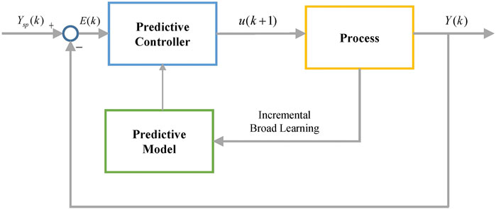
FIGURE 3. Incremental broad learning based predictive control scheme.

4 Benchmark Study on Continuous Stirred Tank Heater

In this section, the proposed predictive control is applied to tune the temperature in the continuous stirred tank heater (CSTH) benchmark. The performance of the proposed control strategy is compared with the partial form dynamic linearization aided model free control (PFDL-MFC) strategy proposed in Hou and Jin (2013) and Hou and Jin (2011). The PFDL-MFC algorithm is chosen for comparison because both algorithms need little prior knowledge of the system model and calculate the optimal control input sequence based on Eq. 4.

The continuous stirred tank heater (CSTH) is a typical pilot plant for control performance evaluation and process monitoring. The experimental CSTH system is developed in the Automation Laboratory at Department of Chemical Engineering, IIT Bombay as shown in Figure 4 (Thornhill et al., 2008). It mainly consists of two separated water storage tanks. The water is heated separately and recycled between the two tanks. The CSTH benchmark can be regarded as a 5-input-3-output system. u₁, u₂, and u₃ represent the inputs controlled by separate valves. u₄ and u₅ represent the outputs of two heaters. The three outputs are the water temperature T₁ (Tank 1), T₂ (Tank 2) and the water level h₂ (Tank 2), respectively. Table 1 gives the parameters of the CSTH benchmark in steady state.

FIGURE 4

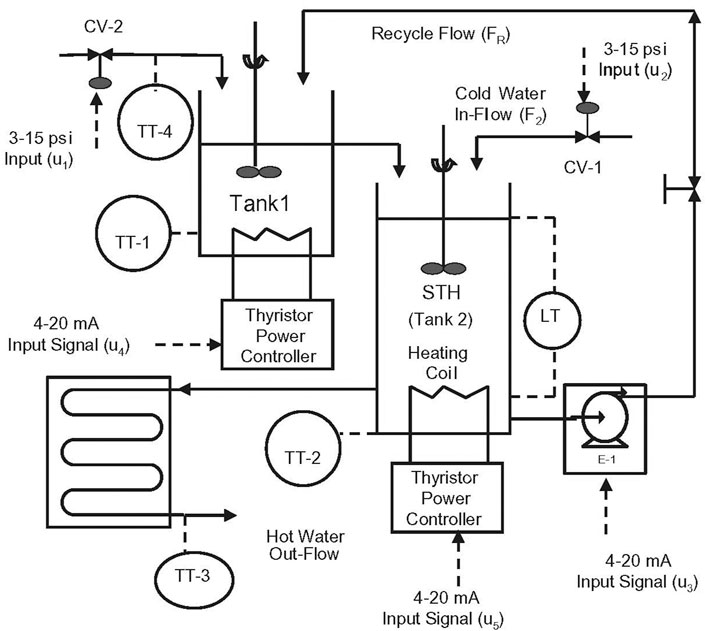
FIGURE 4. CSTH system in IIT Bombay.

TABLE 1

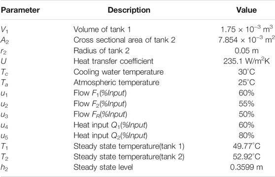
TABLE 1. Nominal model parameters and steady state.

Consider that the heat input is added to the state variables in the form of polynomial functions (Thornhill et al.,2008), the controlled system is nonlinear even if the flow rate is steady. For simplicity, we only use u₄ and u₅ as the controller outputs to be calculated. The designed predictive controller aims to make T₁ track its setpoint. If not specified, the other variables are set to be steady state in Table 1. The practical constraints in the CSTH benchmark are set to be

$\begin{array}{cc}\hfill 0\le & u\le 100\hfill \\ \hfill -0.2\le & \mathrm{\Delta }u\le 0.2\hfill \end{array}.(61)$

Smooth approximation is a popular method to enhance the tracking performance (Chi and Liang, 2015). By smooth approximation, the setpoint can be changed smoothly from one desired state to the other. In the simulation, the setpoint is given as

$y_{sp}\left(k\right)=\left\{\begin{array}{cc}\hfill & y_{s1},0<k\le 800\hfill \\ \hfill & {\lambda }_{sp}{y}_{sp}\left(t-1\right)+\left(1-{\lambda }_{sp}\right)y_{s2},800<k\le 1400\hfill \\ \hfill & {\lambda }_{sp}{y}_{sp}\left(t-1\right)+\left(1-{\lambda }_{sp}\right)y_{s1},1400<k\le 2000\hfill \end{array}\right.,$

where y_s1 = 49, y_s2 = 50 and the smoothing coefficient λ_sp is set to be 0.98.

Consider that the proposed predictive control requires initializing its predictive model based on the available process data. In this simulation, the process inputs are set to be random square waves with white noise in the first 200 s. The initial predictive model is calculated using the process data collected in the first 200 s. After the 200^th instant, the predictive model is updated based on the online process data.

Define the prediction error E_p at the instant k as

$E_p\left(k\right)=\frac{{\sum }_{i=1}^{n_p}\Vert y\left(k+i\right)-y\left(k+i|k\right){\Vert }^2}{n_p}.(62)$

where n_c and n_p are both set to be 50.

Other parameters in the PF-MFPC algorithm are respectively set to be λ = 27, μ = 1, ρ = [1, 1, 1], η = 1, and L = 3. The illustrations of the designed parameters are shown in Table 2. The comparison of the prediction error is shown in Figures 5, 6, from which it can be seen that there exists a fluctuation at the 200^th, 800^th, and 1400^th instant. The fluctuation is caused by the setpoint change. Therefore, both algorithms need to update the model dynamics based on the online process data. The comparison shows that the prediction of the proposed control strategy converges much faster than the PFDL-MFC algorithm. In addition, the fluctuation peaks of the proposed broad learning aided MPC is also much lower than the PFDL-MFC algorithm.

TABLE 2

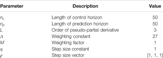
TABLE 2. Illustration of the designed parameters.

FIGURE 5

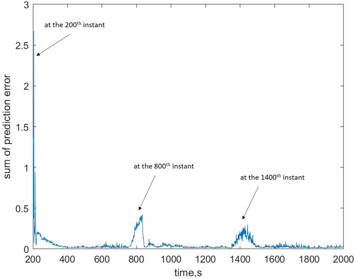
FIGURE 5. Prediction error of broad learning aided predictive control.

FIGURE 6

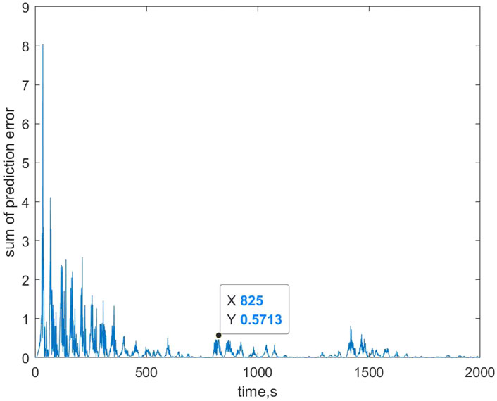
FIGURE 6. Prediction error of PFDL-MFC algorithm.

It is worth mentioning that the fluctuation of E_p occurs before the setpoint changes at the 1400^th and 4800^th instant since the proposed predictive controller is based on the multi-step prediction. In this simulation, it holds that n_c = n_p = 50, which implies that the prediction of the output and the incremental of the input can be foreseen in the future 50 sample instants.

The control performance of the proposed broad learning aided MPC and the PFDL-MFC algorithm are demonstrated in Figures 7, 8, respectively. As the setpoint changes, the input signal converges after a few steps of adjustment. Both algorithms show the efficiency in the tracking control for nonlinear systems. However, the proposed algorithm converges much faster than the PFDL-MFC algorithm though it requires to collect the data during the first several instants. In addition, the parameters of the PFDL-MFC algorithm have a great influence on the control performance. In contrast, only the weight λ₁, λ₂ and the prediction horizon n_p can be adjustable in the proposed predictive control strategy, which shows minor influence on the control performance.

FIGURE 7

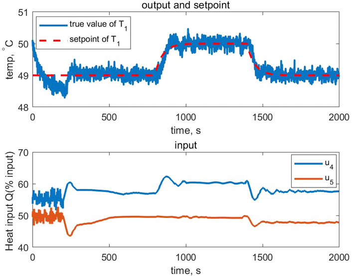
FIGURE 7. Control performance of broad learning aided predictive control.

FIGURE 8

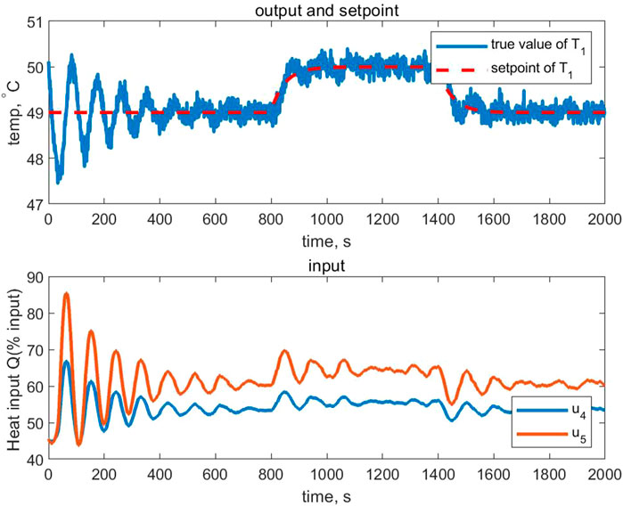
FIGURE 8. Control performance of PFDL-MFC algorithm.

5 Conclusion

This paper proposes a broad learning based data-driven predictive control strategy without any prior knowledge of the system model. The online computation load of the proposed predictive controller is reduced by using the incremental broad learning algorithm. In addition, the prediction precision is enhanced by approximating the predictive model using a Jacobian matrix. The convergence of the predictive control strategy is discussed theoretically, which demonstrates that the approximation has no influence on the convergence of the predictive control algorithm. The effectiveness of the proposed broad learning based MPC is demonstrated for temperature adjustment through the continuous stirred tank heater benchmark.

Compared with other NN based predictive control strategies, the proposed strategy can update the predictive model online with less online computation burden. Meanwhile, the proposed predictive controller generates the local nonlinearity between the input and output data compared with the dynamic linearization based model free control strategy, which enhances the prediction precision and control performance. The simulation result shows that the proposed predictive control strategy shows faster convergence both in the control performance and the prediction than the PFDL-MFC algorithm. In the future, more work can be done to further reduce the online computation burden.

Data Availability Statement

Publicly available datasets were analyzed in this study. This data can be found here: http://www.ps.ic.ac.uk/∼nina/CSTHSimulation/index.htm.

Author Contributions

MT and TG: conceptualization, methodology, writing. XL: supervision. KL: writing. All authors contributed to the article and approved the submitted version.

Conflict of Interest

The authors declare that the research was conducted in the absence of any commercial or financial relationships that could be construed as a potential conflict of interest.

Publisher’s Note

All claims expressed in this article are solely those of the authors and do not necessarily represent those of their affiliated organizations, or those of the publisher, the editors and the reviewers. Any product that may be evaluated in this article, or claim that may be made by its manufacturer, is not guaranteed or endorsed by the publisher.

Acknowledgments

This work is funded by Open Foundation of Science and Technology on Thermal Energy and Power Laboratory under Grant TPL2018C02.

References

Chen, C. L. P., and Liu, Z. (2018). Broad Learning System: An Effective and Efficient Incremental Learning System without the Need for Deep Architecture. IEEE Trans. Neural Netw. Learn. Syst. 29, 10–24. doi:10.1109/tnnls.2017.2716952

PubMed Abstract | CrossRef Full Text | Google Scholar

Chen, C. L. P., and Wan, J. Z. (1999). A Rapid Learning and Dynamic Stepwise Updating Algorithm for Flat Neural Networks and the Application to Time-Series Prediction. IEEE Trans. Syst. Man. Cybern. B 29, 62–72. doi:10.1109/3477.740166

CrossRef Full Text | Google Scholar

Chi, Q., and Liang, J. (2015). A Multiple Model Predictive Control Strategy in the Pls Framework. J. Process Control. 25, 129–141. doi:10.1016/j.jprocont.2014.12.002

CrossRef Full Text | Google Scholar

Díaz-García, J. A., and Gutiérrez-Jáimez, R. (2006). Distribution of the Generalised Inverse of a Random Matrix and its Applications. J. Stat. Plann. Inference 136, 183–192. doi:10.1016/j.jspi.2004.06.032

CrossRef Full Text | Google Scholar

Gao, T., Yin, S., Qiu, J., Gao, H., and Kaynak, O. (2018). A Partial Least Squares Aided Intelligent Model Predictive Control Approach. IEEE Trans. Syst. Man. Cybern, Syst. 48, 2013–2021. doi:10.1109/tsmc.2017.2723017

CrossRef Full Text | Google Scholar

Garcia-Torres, F., Bordons, C., and Ridao, M. A. (2019). Optimal Economic Schedule for a Network of Microgrids with Hybrid Energy Storage System Using Distributed Model Predictive Control. IEEE Trans. Ind. Electron. 66, 1919–1929. doi:10.1109/tie.2018.2826476

CrossRef Full Text | Google Scholar

Garg, A., and Mhaskar, P. (2017). Subspace Identification and Predictive Control of Batch Particulate Processes.”in American Control Conference (ACC). doi:10.23919/acc.2017.7963003

CrossRef Full Text | Google Scholar

Gong, M., Liu, J., Li, H., Cai, Q., and Su, L. (2015). A Multiobjective Sparse Feature Learning Model for Deep Neural Networks. IEEE Trans. Neural Netw. Learn. Syst. 26, 3263–3277. doi:10.1109/tnnls.2015.2469673

PubMed Abstract | CrossRef Full Text | Google Scholar

Guo, P., He, Z., Yue, Y., Xu, Q., Huang, X., Chen, Y., et al. (2019). A Novel Two-Stage Model Predictive Control for Modular Multilevel Converter with Reduced Computation. IEEE Trans. Ind. Electron. 66, 2410–2422. doi:10.1109/tie.2018.2868312

CrossRef Full Text | Google Scholar

Han, H.-G., Zhang, L., Hou, Y., and Qiao, J.-F. (2016). Nonlinear Model Predictive Control Based on a Self-Organizing Recurrent Neural Network. IEEE Trans. Neural Netw. Learn. Syst. 27, 402–415. doi:10.1109/tnnls.2015.2465174

PubMed Abstract | CrossRef Full Text | Google Scholar

Hidalgo, P. M., and Brosilow, C. B. (1990). Nonlinear Model Predictive Control of Styrene Polymerization at Unstable Operating Points. Comput. Chem. Eng. 14, 481–494. doi:10.1016/0098-1354(90)87022-h

CrossRef Full Text | Google Scholar

Hoerl, A. E., and Kennard, R. W. (2000). Ridge Regression: Biased Estimation for Nonorthogonal Problems. Technometrics 42, 80–86. doi:10.1080/00401706.2000.10485983

CrossRef Full Text | Google Scholar

Hou, Z., and Jin, S. (2011). A Novel Data-Driven Control Approach for a Class of Discrete-Time Nonlinear Systems. IEEE Trans. Contr. Syst. Technol. 19, 1549–1558. doi:10.1109/tcst.2010.2093136

CrossRef Full Text | Google Scholar

Hou, Z., and Jin, S. (2013). Model Free Adaptive controlTheory and Applications. CRC Press,Taylor & Francis Group.

Google Scholar

Kaspar, M. H., and Harmon Ray, W. (1993). Dynamic PLS Modelling for Process Control. Chem. Eng. Sci. 48, 3447–3461. doi:10.1016/0009-2509(93)85001-6

CrossRef Full Text | Google Scholar

Kou, P., Feng, Y., Liang, D., and Gao, L. (2019). A Model Predictive Control Approach for Matching Uncertain Wind Generation with PEV Charging Demand in a Microgrid. Int. J. Electr. Power Energ. Syst. 105, 488–499. doi:10.1016/j.ijepes.2018.08.026

CrossRef Full Text | Google Scholar

Li, K., Luo, H., Yang, C., and Yin, S. (2020). Subspace-aided Closed-Loop System Identification with Application to DC Motor System. IEEE Trans. Ind. Electron. 67, 2304–2313. doi:10.1109/tie.2019.2907447

CrossRef Full Text | Google Scholar

Mayne, D. Q., and Rawlings, J. B. (2001). Correction to "Constrained Model Predictive Control: Stability and Optimality". Automatica 37, 483. doi:10.1016/s0005-1098(00)00173-4

CrossRef Full Text | Google Scholar

Meidanshahi, V., Corbett, B., Adams, T. A., and Mhaskar, P. (2017). Subspace Model Identification and Model Predictive Control Based Cost Analysis of a Semicontinuous Distillation Process. Comput. Chem. Eng. 103, 39–57. doi:10.1016/j.compchemeng.2017.03.011

CrossRef Full Text | Google Scholar

Patwardhan, R. S., Lakshminarayanan, S., and Shah, S. L. (1998). Constrained Nonlinear Mpc Using Hammerstein and Wiener Models: Pls Framework. Aiche J. 44, 1611–1622. doi:10.1002/aic.690440713

CrossRef Full Text | Google Scholar

Qin, S. J., and Badgwell, T. A. (2003). A Survey of Industrial Model Predictive Control Technology. Control. Eng. Pract. 11, 733–764. doi:10.1016/s0967-0661(02)00186-7

CrossRef Full Text | Google Scholar

Rossiter, J. (2003). Model-based Predictive Control: A Practical Approach. Boca Raton, Florida): CRC Press.

Google Scholar

Thornhill, N. F., Patwardhan, S. C., and Shah, S. L. (2008). A Continuous Stirred Tank Heater Simulation Model with Applications. J. Process Control. 18, 347–360. doi:10.1016/j.jprocont.2007.07.006

CrossRef Full Text | Google Scholar

Wu, X., Shen, J., Li, Y., and Lee, K. Y. (2013). Data-Driven Modeling and Predictive Control for Boiler-Turbine Unit. IEEE Trans. Energ. Convers. 28, 470–481. doi:10.1109/tec.2013.2260341

CrossRef Full Text | Google Scholar

Yi, L. (20162016). “System Modeling and Identification of Unmanned Quad Rotor Air Vehicle Based on Subspace and Pem,” in IEEE Systems And Technologies For Remote Sensing Applications through Unmanned Aerial Systems (STRATUS). doi:10.1109/stratus.2016.7811137

CrossRef Full Text | Google Scholar

Yin, S., and Xiao, B. (2017). Tracking Control of Surface Ships with Disturbance and Uncertainties Rejection Capability. Ieee/asme Trans. Mechatron. 22, 1154–1162. doi:10.1109/tmech.2016.2618901

CrossRef Full Text | Google Scholar

Yin, S., Yu, H., Shahnazi, R., and Haghani, A. (2017). Fuzzy Adaptive Tracking Control of Constrained Nonlinear Switched Stochastic Pure-Feedback Systems. IEEE Trans. Cybern. 47, 579–588. doi:10.1109/tcyb.2016.2521179

PubMed Abstract | CrossRef Full Text | Google Scholar

Yu, H., Xie, T., Paszczynski, S., and Wilamowski, B. M. (2011). Advantages of Radial Basis Function Networks for Dynamic System DesignIEEE Trans. Ind. Electron. 58, 5438–5450. IEEE International Conference on Mechatronics (ICM 2009)APR 14-17, 2009. doi:10.1109/tie.2011.2164773

CrossRef Full Text | Google Scholar

Yuzgec, U., Becerikli, Y., and Turker, M. (2008). Dynamic Neural-Network-Based Model-Predictive Control of an Industrial Baker's Yeast Drying Process. IEEE Trans. Neural Netw. 19, 1231–1242. doi:10.1109/tnn.2008.2000205

CrossRef Full Text | Google Scholar

Zhang, Y., Xu, D., and Huang, L. (2018). Generalized Multiple-Vector-Based Model Predictive Control for PMSM Drives. IEEE Trans. Ind. Electron. 65, 9356–9366. doi:10.1109/tie.2018.2813994

CrossRef Full Text | Google Scholar

Zhou, P., Dai, P., Song, H., and Chai, T. (2017). Data‐driven Recursive Subspace Identification Based Online Modelling for Prediction and Control of Molten Iron Quality in Blast Furnace Ironmaking. IET Control. Theor. Appl. 11, 2343–2351. doi:10.1049/iet-cta.2016.1474

CrossRef Full Text | Google Scholar