Path Planning for a Jumping Rover Team With a Charging Station in Multi-Waypoints Visiting Missions

1 Introduction

Unmanned ground vehicles (UGVs) have been used extensively for exploration in unknown or dangerous environments where humanity is not able to access. The terrain in the exploration mission may consist of diversified features, such as flats, cliffs, and slopes. For most of the exploration missions, a UGV is selected according to the specific feature of the overall terrain. For example, wheeled robots have been used to travel to the target location in environments with flat terrain. However, for terrain with complicated geometry, the exploration mission is performed by particular types of locomotive, such as caterpillar tracked robots or unmanned aerial vehicles (UAVs). Although general wheeled UGVs show extended operational time in most cases, they cannot overcome obstacles, such as areas with large gaps or terrain with high elevations. UAVs, on the other hand, are subject to atmospheric effects and are governed by more stringent safety or operational requirements. Considering the limitations of traditional UAVs and UGVs, we propose using a team of wheeled robots with jumping capabilities for multi-waypoints visiting missions with obstacles. The focus is to develop an optimal path planning algorithm for the particular robot team to search for the energy-efficient path in the assigned mission.

Compared to a traditional wheeled vehicle that has to avoid obstacles, the jumping capability provides flexibility on path planning, as a jumping rover can decide whether to avoid or jump over/onto the obstacles. The jumping motion is achieved by deforming the robot’s parts, e.g., wheels (Ye et al., 2018), or activating their jumping apparatus (Mizumura et al., 2017). In the space industry, hopping robots have been applied in planetary exploration missions (Morad et al., 2018; Hockman and Pavone, 2020). Existing studies on the control of a jumping robot focus on generating precise jumping motion, e.g., legged motion with specific speed and torque (Ding and Park, 2017) and motion control of a jumping robot that uses a tail as its jumping mechanism (Iwamoto and Yamamoto, 2015). The motion planning approach for a jumping robot has been developed that prioritizes safety and minimizes the cost of jumping by finding an optimal landing position (Ushijima et al., 2017). And obstacles are treated as a point that cannot be used as a suitable landing surface in the literature. In this paper, we consider specific dimensions of an obstacle that can be landed by a jumping rover.

Another concern that restricts the robot motion in traveling missions is the limited battery capacity, especially in long-term operations. Therefore, to extend the operational time in traveling missions, charging stations have been considered to provide extra power within the mission area. In ideal scenarios, a charging station will allow rovers to work persistently (Mathew et al., 2015; Kingry et al., 2017). When a charging station is considered in the multi-waypoints visiting mission, the path planning problem is more challenging as we need to consider paths from/to a charging station in addition to the paths between the target locations. Furthermore, charging decisions, e.g., which rover should be charged and when to charge them (Michaud and Robichaud, 2002), need to be determined based on the assigned mission and energy consumption rate. These charging stations are required to automatically connect to the inlet of an autonomous robot. Work in (Behl et al., 2019) utilized a camera to detect the relative position between a charging plug and a robot. Another work in (Barzegaran et al., 2017) utilized wireless power transmission for electric vehicles. Due to the size and weight limitation of the jumping rover, we cannot apply those charging methods to connect with the jumping rover. Instead, magnetic connectors are introduced to connect two end effectors of a station and a rover.

Many types of route optimization algorithms have been developed to solve path planning problems involving multiple robots, e.g., dynamic programming (Kok et al., 2010; Ou and Sun, 2010), minimum spanning tree algorithms (Pettie and Ramachandran, 2002), Tabu search (Archetti et al., 2006), ant colony optimization (Abousleiman et al., 2017), and particle swarm optimization (Belmecheri et al., 2013). A general multi-waypoints traveling mission performed by a team of robots can be formulated as the well-known multi traveling salesperson problem (mTSP) and then solved via the mixed-integer linear programming (MILP) algorithm, which is not directly applicable to the path planning problem considered in this paper. One reason is the involvement of a charging station, which requires determining visiting sequences and time to a charging station. The other reason is the inclusion of obstacles, which complicates the traditional mTSP. The development of motion planning methods has led to various techniques being used, including sampling-based algorithms such as probabilistic road map (PRM) (Kavraki et al., 1996) and rapidly exploring random tree (RRT) (LaValle, 1998; LaValle and Kuffner Jr, 2001). A variant of RRT, named RRT∗, iteratively searches for an optimized solution, e.g., shortest path (Karaman et al., 2011). In this paper, after obtaining a path using the basic RRT∗ algorithm, path refinement techniques are proposed to search for an optimal path that meets the jumping rover’s motion constraint.

Based on our prior work of jumping rovers (Tan et al., 2020), this work extends the jumping rover team with a charging station and proposes new algorithms for path planning and task allocation. We first find energy-efficient path segments between any two target locations by a refined RRT∗ algorithm, where an obstacle can be treated as a possible pathway if a jumping rover is able to jump over it. If there are obstacles between two targets, the refined RRT∗ determines whether avoiding obstacles or jumping over obstacles is more energy efficient. We then utilize the genetic algorithm (GA) to search for the most profitable combination of path segments to visit all targets, as well as path segments to/from the charging station to satisfy energy constraints. When considering the charging station and energy constraints of each jumping rover, it makes the path planning of the multi-waypoints traveling mission much more challenging, which requires a new formulation and path planning method incorporating the charging function and energy constraints. Compared to our prior work in (Tan et al., 2020), the contribution of this paper includes the following points: (1) a new formulation of the multi-waypoints traveling mission of a robot team integrating the charging function and energy constraints. (2) a path planning algorithm with refined paths that consider more complicated geometries of an obstacle in both rolling and jumping motion, (3) introducing GA to determine both visiting and charging sequences, and (4) design and construction of a charging system that automatically docks with the jumping rovers.

The paper is organized as follows: Section 2 introduces the robot team and problem formulation, Section 3 describes the development of path planning and task allocation algorithm. The simulation and experimental results are presented in Section 4. Finally, we address the conclusions and future work in Section 5.

2 Robot Team Model and Problem Statement

2.1 Jumping Rovers and Charging Station

There are multiple requirements to verify the improved mobility and energy efficiency of a jumping rover team in real-world operations. First and foremost, the rolling motion must produce ground-based locomotion and the jumping motion is required to produce vertical displacement. Second, it must record energy consumption from both types of motion to validate the proposed algorithm properly. The wheeled, jumping rovers are based upon a Parrot Jumping Sumo robot chassis (Parrot, 2019). The rover is made out of different materials, including acrylic, nylon, aluminum, and 3D printed parts because the rover must be lightweight to achieve an acceptable jumping height. The center of mass sits on the force vector of the jumping mechanism to ensure the rover does not flip after actuation. In addition, “whiskers” in the front enable the rover to descend from the top of obstacles without flipping over. Each jumping rover has a fixed jumping height determined by the stiffness of the compressed spring. Two jumping rovers with different energy consumption rates and jumping heights are demonstrated in Figure 1A. The left rover in Figure 1A can jump higher and consumes more energy than the other one.

FIGURE 1

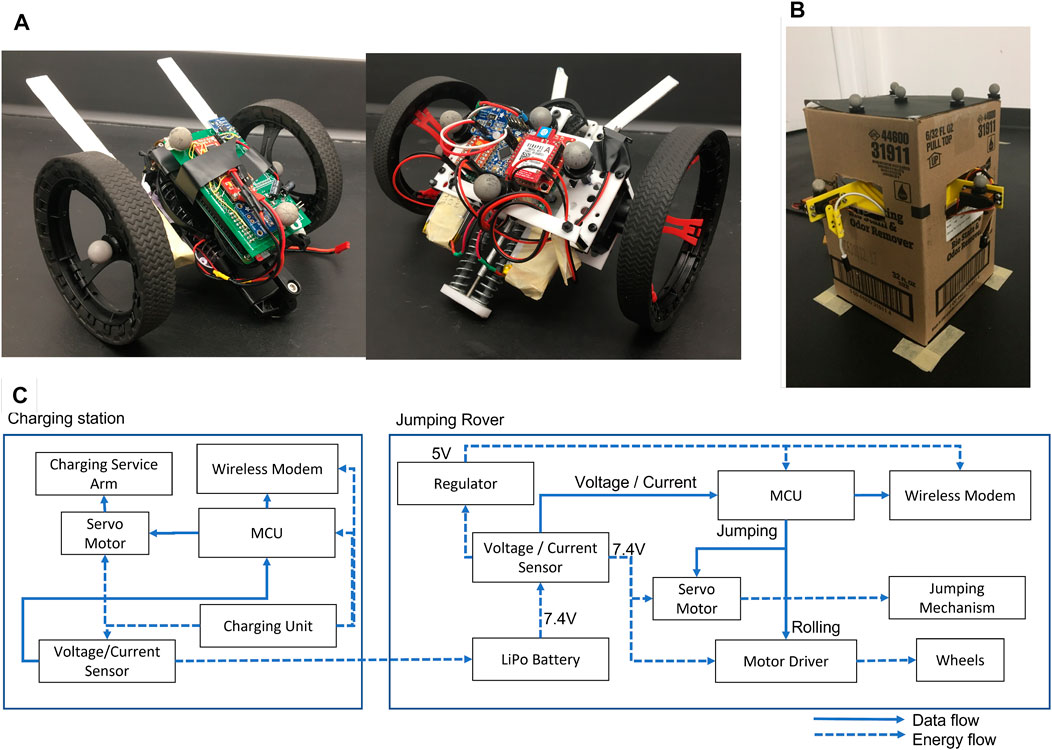
FIGURE 1. Jumping rovers and charging station (A): jumping rover 1 (UGV 1) (left) and jumping rover 2 (UGV 2) (right), (B): charging Station (C): overall data and power flow.

The charging station is built to automatically charge the two rovers, as shown in Figure 1B. Each rover has a unique charging port and the charging station has two charging port arms. The charging service arms can rotate to capture the port of the rover. Moreover, magnet tips are used for the charging station outlets to secure the docking of rovers with the charging station via magnetic forces. We use the “HX-A3 Hexfly Lipo Battery Charger” for each rover. Depending on the battery level of the rover, the charging time can be different for the same amount of charged energy. We also use voltage and current sensors to measure how much energy is provided to the rover from the chargers and these measurements are transmitted to the mission control computer via a wireless modem.

The Parrot Jumping Sumo robot that can be purchased off the shelf is a manually operated rover. The overall system is shown in Figure 1C. We modified the original model with a Micro controller Unit (MCU) and communication system to achieve autonomous operation, including a customized jumping mechanism. The jumping rovers are controlled wirelessly through serial communication with a mission control computer. The commands are then relayed to a motor driver that controls the rotational speed of the wheel motors. Signals for the jumping mechanism are applied directly from the MCU to a servo motor. Each rover and the charging station have voltage and current sensors to measure its power consumption or charging power. Waypoints for the planned path are output from the MATLAB simulation and followed by the physical UGV through a 3D space coordinate measured by a motion capture system.

2.2 Rover’s Kinematics and Control

In order to make the rovers follow the desired trajectories, we use the basic kinematics of the two-wheeled robot (Ichihara and Ohnishi, 2006; Chen et al., 2008). The rolling and jumping motion working mechanism is shown in Figures 2A,B. For the rolling motion, its coordinate is represented by X and Y. The center point velocity of the rover is denoted by v. Then, $\dot{X}$ and $\dot{Y}$ are expressed as,

$\begin{array}{ccc}\hfill \dot{X}=v\cos \theta & \hfill & \hfill \\ \hfill \dot{Y}=v\sin \theta & \hfill & \hfill \end{array}(1)$

where θ is the heading angle of the rover and the angular velocity ω is the heading angle changing rate, denoted by $\dot{\theta }$. Then, we can express the velocity terms in a matrix form, expressed as

$\left[\begin{array}{c}\hfill \dot{X}\hfill \\ \hfill \dot{Y}\hfill \\ \hfill \dot{\theta }\hfill \end{array}\right]=\left[\begin{array}{cc}\hfill \cos \theta \hfill & \hfill 0\hfill \\ \hfill \sin \theta \hfill & \hfill 0\hfill \\ \hfill 0\hfill & \hfill 1\hfill \end{array}\right]\left[\begin{array}{c}\hfill v\hfill \\ \hfill \omega \hfill \end{array}\right](2)$

FIGURE 2

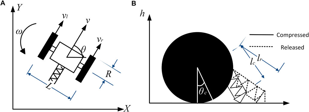
FIGURE 2. Jumping rover’s motion (A) rolling motion, (B) jumping motion.

The relationship between the translational and angular velocity of the rover and the translational velocities (v_l, v_r) of each wheel can be expressed by

$\left[\begin{array}{c}\hfill v\hfill \\ \hfill \omega \hfill \end{array}\right]=\left[\begin{array}{cc}\hfill \frac{1}{2}\hfill & \hfill \frac{1}{2}\hfill \\ \hfill \frac{1}{L}\hfill & \hfill -\frac{1}{L}\hfill \end{array}\right]\left[\begin{array}{c}\hfill v_r\hfill \\ \hfill v_l\hfill \end{array}\right]=\left[\begin{array}{cc}\hfill \frac{R}{2}\hfill & \hfill \frac{R}{2}\hfill \\ \hfill \frac{R}{L}\hfill & \hfill -\frac{R}{L}\hfill \end{array}\right]\left[\begin{array}{c}\hfill {\omega }_r\hfill \\ \hfill {\omega }_l\hfill \end{array}\right](3)$

where L is the width of the rover, and ω_l and ω_r are the angular velocity of the left and right wheel, respectively. Then, we can derive the relationship between the velocity and the angular velocity of the wheel.

$\left[\begin{array}{c}\hfill \dot{X}\hfill \\ \hfill \dot{Y}\hfill \\ \hfill \dot{\theta }\hfill \end{array}\right]=\left[\begin{array}{cc}\hfill \frac{R}{2}\cos \theta \hfill & \hfill \frac{R}{2}\cos \theta \hfill \\ \hfill \frac{R}{2}\sin \theta \hfill & \hfill \frac{R}{2}\sin \theta \hfill \\ \hfill \frac{R}{L}\hfill & \hfill -\frac{R}{L}\hfill \end{array}\right]\left[\begin{array}{c}\hfill {\omega }_r\hfill \\ \hfill {\omega }_l\hfill \end{array}\right](4)$

This relationship shows that the rover’s motion is non-holonomic. For the rolling motion, the four differential-drive primitives of a Balkcom-Mason curve are considered to simplify its motion with straight line and zero-radius rotation. When the rover changes its heading, time and energy consumption for rotation are negligible. Therefore, only line segment driving is considered when calculating the energy consumption.

Due to the limited size of rovers and weight limit for the jumping motion, there are no encoders implemented in the rovers to measure the rotational speed of their wheels. Therefore, to adjust the rovers’ heading angle, their wheel speed is under control such that the rovers can maintain their heading angle when following a straight line. A proportional and derivative controller is applied to maintain a desired heading angle, expressed as

$u=K_{p}e\left(\theta \right)+K_d\frac{de\left(\theta \right)}{dt}(5)$

where u is the differential input for the rotational speed of a rover, e(θ) is the error of angle between a desired heading angle and the current heading angle, and k_p and k_d are the proportional and derivative gains, respectively.

For the jumping motion, we need to determine the maximum jumping height based on the energy conservation principle. By calculating the spring potential energy, the maximum jumping height can be determined by,

$h_{\text{max}}=\frac{k_{\text{spring}}{\left(\left(l_r-l_c\right)\mathrm{c}\mathrm{o}\mathrm{s}{\theta }_c\right)}^2}{2W}(6)$

where k_spring is the spring constant, l_r is the spring length when it is released, l_c is the spring length when it is compressed, θ_c is the angle between the rover and the vertical axis, and W is the weight of the rover. The characteristics of energy consumption and jumping capability of two rovers are shown in Table 1, where UGV 1 jumps higher than UGV 2 and consumes about four times as much energy as UGV 2 for every jump.

TABLE 1

TABLE 1. Energy and jumping characteristics of UGVs.

2.3 Problem Statement

The objective for a team of UGVs is to visit a set of targets using the most energy-efficient route, where one stationary charging station is provided for the power supply. The targets are denoted as T = T_{{1,2,…, m}}, where m is the total number of visiting targets. The charging station is denoted by S. All UGVs start at T₁ and rendezvous at the same destination. The m targets can be located anywhere in the mission area, including the top of obstacles. In addition to the specified targets, we consider n obstacles randomly scattered in the mission area, denoted by O = O_{{1,2,…, n}}. Each obstacle is a rectangular prism with a flat surface and given dimensions. These obstacles are treated as solid objects that cannot be passed through or moved. They will not overlap with each other; however, their boundaries can intersect adjacent ones such as O₄, O₅, and O₆ shown in Figure 3. The UGVs are indexed as z = 1, 2, …, p. UGVs in the team can reach different jumping heights. To generate a feasible jumping path, we need to consider the kinematics of two-wheeled vehicles and the obstacles’ geometry. The jumping path associated with an obstacle is positioned perpendicular to the border of the obstacle. Each target point can only be visited by one UGV to reduce the cost associated with the travel, except for the initial and the destination targets. The number of visiting a charging station is not limited.

FIGURE 3

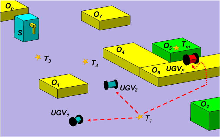
FIGURE 3. Mission overview.

Consider a single UGV that operates with two operational modes. One is the rolling mode that rotates motors as a general ground vehicle, and the other mode is the jumping mode. The UGV stops at the jumping position and compresses and releases its spring mechanism to jump. With a constant velocity during straight forward rolling and constant angular speed during zero radii rotation for UGV z, z = 1, …, p, the energy consumption rate of the jumping rover in straight forward motions is denoted by $P_z^l$. The energy consumption for straight forward and jumping motion is much higher than the one required for rotation, which makes the energy consumption for rotating motion negligible. In addition, the passive energy drawn from the vehicle’s electronic components, such as the MCU, is a fixed value and denoted by $P_z^a$. The height of the jumping motion for each UGV is held constant, denoted by h_z, with fixed energy expenditure, denoted by J_z, associated with the corresponding jumping rover z = 1, …, p. The energy consumption for each jumping rover traveling from target i to target j, i, j = 1, …, m, i ≠ j, is determined by

$c_{ij,z}=\left(P_z^l+P_z^a\right)t_{ij,z}^l+J_z{N}_{ij,z},(7)$

where $t_{ij,z}^l$ is the time duration along the rolling motion between targets i and j, N_ij,z is the overall number of jumps for UGV z, z = 1, …, p, between targets i and j. The time used to travel between two targets can be calculated by the velocity of each rover and the distance between the targets, where constant velocity is used for each rover. By adding the energy consumption of all jumping rovers along path segments connecting all targets, we can find the overall UGV team energy usage during the visiting mission.

In this paper, each UGV is confined to the energy consumption constraint due to the limited battery capacity. Therefore, a UGV needs to visit the charging station before its stored energy becomes exhausted. Assuming the energy initially stored in the battery for each UGV is E_0,z, a UGV’s stored energy will reach the initial amount every time it is charged at the station. Before approaching the charging station, a designated UGV should have sufficient energy to drive to the charging station. During the charging process, ΔE_l,z amount of energy is provided from the station at the lth charging sequence to UGV z such that the stored energy will reach the initial amount.

The path planning problem for the multi-waypoints visiting mission can be represented by a complete graph $\mathcal{G}=(\mathcal{V},\mathcal{E})$ which consists of a set $\mathcal{V}=T_{\{\mathrm{1,2},\dots ,m\}}\cup S$ as graph vertices and an edge set $\mathcal{E}$ connecting any two target points. The associated edge cost for $(i,j)\in \mathcal{E}$ is determined by the energy consumption amount required to travel from target i to j, where i, j = 1, 2, …, m, S and i ≠ j. In addition, x_ij,z is a binary variable that is determined by

$x_{ij,z}=\left\{\begin{array}{cc}1,\hfill & \text{edge}\left(i,j\right)\in \mathcal{E}\text{will\hspace{0.17em}be\hspace{0.17em}visited\hspace{0.17em}by\hspace{0.17em}UGV}z\hfill \\ 0,\hfill & \text{edge}\left(i,j\right)\in \mathcal{E}\text{will\hspace{0.17em}not\hspace{0.17em}be\hspace{0.17em}visited\hspace{0.17em}by\hspace{0.17em}UGV}z\hfill \end{array}\right.$

All vehicles start at the first target, denoted as T₁, and end at the same destination point T_k, where the index k, 1 < k ≤ m, is unknown and will be determined by the path planning algorithm. T′ is a set of targets excluding the initial target such that T = T₁ ∪ T′. Let V_z be the collection of target indices, excluding the charging station, visited by UGV z, where elements of V_z, are sorted according to the visiting sequences. The number of targets, excluding the charging station, visited by UGV z is denoted as n_z, which is also the length of V_z. Then, the path planning problem for the energy-efficient multi-waypoints visiting mission can be formulated as

$\begin{array}{ccc}\hfill & \hfill & \min \sum _{z=1}^p\sum _{j\in T^{\prime },j\ne i}\sum _{i\in T\cup S}{c}_{ij,z}{x}_{ij,z}\hfill \end{array}(8)$

$\begin{array}{ccc}\hfill \text{s.t.}& \hfill & \sum _{z=1}^p\sum _{j\in T^{\prime }\cup S}{x}_{1j,z}=p\hfill \end{array}(9)$

$\begin{array}{ccc}\hfill & \hfill & \sum _{z=1}^p\sum _{j\in T^{\prime }\cup S}{x}_{jk,z}=p,j\ne k,k\in T^{\prime }\hfill \end{array}(10)$

$\begin{array}{ccc}\hfill & \hfill & \sum _{z=1}^p\sum _{i\in T\cup S}{x}_{ij,z}=1,j\in T^{\prime },i\ne j,j\ne k\hfill \end{array}(11)$

$\begin{array}{ccc}\hfill & \hfill & \sum _{z=1}^p\sum _{j\in T\cup S}{x}_{ij,z}=1,i\in T^{\prime },i\ne j,i\ne k\hfill \end{array}(12)$

$\begin{array}{ccc}\hfill & \hfill & \sum _{i,j\in V_z}\left(x_{iS,z}-x_{Sj,z}\right)=0,z=1,\dots ,p\hfill \end{array}(13)$

$\begin{array}{ccc}\hfill & \hfill & \sum _{i,j\in V_z\left(1,\dots ,l_z\right)}\left(c_{iS,z}{x}_{iS,z}+c_{ij,z}{x}_{ij,z}+c_{Sj,z}{x}_{Sj,z}-x_{iS,z}\mathrm{\Delta }{E}_{i,z}\right)\le E_{0,z}-E_{\min ,z},\hfill \\ \hfill & \hfill & l_z=2,\dots ,n_z-1,z=1,\dots ,p\hfill \end{array}(14)$

where Eq. 8 is the cost function representing the overall energy consumption for the jumping rover team to visit all the assigned targets, as well as the charging station. Constraints 9, 10 indicate that all p UGVs start at target T₁ and end at target T_k. Constraints 11, 12 require that one target should only be visited once, except for the starting and ending targets and the charging station. Constraint 13 indicates that at least one pair of edges exists to connect the charging station with two adjacent targets i and j in the set of V_z if UGV z visits the charging station. A UGV may visit the charging station multiple times according to its energy consumption characteristics. Constraint (14) specifies that the energy in the battery of each UGV is required to maintain above E_min,z for all the time, where x_iS,zΔE_i,z indicates that if UGV z gets charged after visiting target i, it will gain ΔE_i,z to reach the initial energy amount, denoted as E_0,z, and V_z (1, …, l_z) represents the first l_z elements in the set V_z.

3 Path Planning and Task Allocation Algorithm

The multi-waypoints visiting problem formulated in Eqs 8–14 also needs to consider the n obstacles in the mission area. First, a refined RRT∗ algorithm is proposed to determine the optimized paths between any two target points. Then, a customized GA is applied to search for optimal sequences to visit all the target points, as well as the charging station when it is necessary for a UGV to charge its battery.

3.1 Refined RRT∗

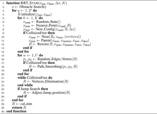
When applying the RRT algorithm (LaValle, 1998; LaValle and Kuffner Jr, 2001) to search for a feasible path, each tree begins at an initial point, x_init, and attempts to make a connection between the origin and a random point, x_rand, in a specified area. The length of the connection is dictated by an established unit length, Δx. The connection of the random point is made with the nearest point in the tree x_near to a new point, x_new, which can be reached. Basically, a unit vector multiplied by a scalar, Δx, in the direction of the random point. This configuration is added to the result data, and a new connection is made without violating the collision constraint. The process is repeated for a number of desired iterations, K, and the selected points in the sequence are saved in R. If the final destination point, x_dest, is provided, then x_dest connects to their nearest random point of a generated tree without violating the collision constraint before the function terminates. While effective in finding a solution with a fast speed, RRT cannot guarantee that solutions are efficient in terms of the length of the tree path from x_init to x_dest. Thus, RRT∗, the optimized version of RRT, takes each point in a tree, finds the points within a radius of each point, and replaces existing edges with the most efficient path without violating the collision constraints.

However, RRT∗ is restricted to optimization within a radius around a vertex or within a “neighborhood.” Due to this limitation, RRT∗ may not provide a smooth solution that is traversable between target locations. To compensate for the deficiency, we propose a refined RRT∗ method with the process shown in Algorithm 1 from line 15 to line 23. We aim to shorten the final path through the refinement process and make it more energy efficient by excluding unnecessary tree segments through the smoothing and elimination process. The smoothing process selects two random points on two distinct edges that link RRT∗ vertices and creates a smoother path that does not violate the collision constraints. The smoothing process continues until it reaches the desired number of smoothing iterations, U. The elimination process checks all edges from the initial to the final vertices. If an edge does not collide with any obstacles, the second vertex together with the edge that links to it will be eliminated, and the third vertex will become the second one. The elimination process removes unnecessary vertices.

Algorithm 1 Refined RRT∗ Algorithm.

With the jumping capability, the jumping rovers can decide whether to jump over or avoid an obstacle. Jumping over an obstacle leads to obstacle elimination and then changes a non-traversable path into a feasible one. Therefore, additional feasible path segments will be created for the multi-waypoints visiting mission with the jumping option. If the number of obstacles lying on the straight line path between targets T_i and T_j is n_f, there will be $2^{n_f}$ number of feasible paths to connect T_i and T_j. For example, in Figure 4, two obstacles are lying on the straight line connecting targets T₁ and T₂. There are four feasible paths between T₁ and T₂.The results from the refined RRT∗ algorithm are affected by the number of samples. To improve the performance of the refined RRT∗ to obtain a result closer to the global optimal solution, it is necessary to examine the effects on the convergence rate and cost value of the refined RRT∗ results when selecting a different number of samples. Using one part of Scenario 3 to find the collision avoidance path between Targets T₂ and T₇ as an analysis example, when changing the number of samples from 300 to 10,000 and running the refined RRT∗ 50 times for each sample number, the convergence rate is shown in Figure 5A. Therefore, at least 4,000 samples are required to guarantee convergence of the refined RRT∗ algorithm. According to the convergence analysis, we assign the minimum number of samples for the refined RRT∗ algorithm according to the effective area including every two targets in the mission. Moreover, the cost value under different numbers of samples is compared. For the original RRT∗ algorithm, it is obvious that the increased number of samples leads to shorter paths with a reduced cost value. For the refined RRT∗ algorithm proposed in this paper, it always obtains a near-optimal solution once it converges, as shown in Figure 5B. With these analysis results, 4,000 samples are assigned when calculating paths between every two targets in the refined RRT∗ algorithm, which guarantees convergence and the converged result is a near-optimal solution.

FIGURE 4

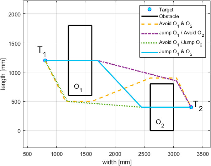
FIGURE 4. Traversable paths between targets 1 and 2 with jumping and avoiding options.

FIGURE 5

FIGURE 5. (A): RRT* convergence rate v.s. number of samples, (B): Cost value v.s. number of samples for RRT* and refined RRT*, (C): GA performance under different combinations of crossover and mutation rates.

3.2 Path Generation for Grouped Obstacles

Section 3.1 considers the cases where obstacles are separated from each other. This section shows the generation of traversable path segments for obstacles that are grouped together. Using the scenario in Figure 3 as an example, obstacles O₄, O₅, and O₆ are grouped together and the elevation of O₅ is higher than the other two adjacent neighbors.

Under such type of scenarios, we need to determine directions to approach and depart the grouped obstacles as well as the routes traveling on top of them. We first approximate every obstacle as a combination of unit blocks. For example, O₄ and O₆ in Figure 6A are composed of three-unit blocks. Moreover, the grouped obstacles are surrounded by the same unit blocks in four directions, denoted as W, S, E, N. Based on the geometry approximation of the grouped obstacles and their surrounding areas, an adjacency matrix is established to represent the adjacency relationship between an obstacle and a surrounding area, as well as the relationship between any two obstacles in the group. For example, the adjacency matrix, dented as A_d, for the case in Figure 6B is shown in Figure 6C.

FIGURE 6

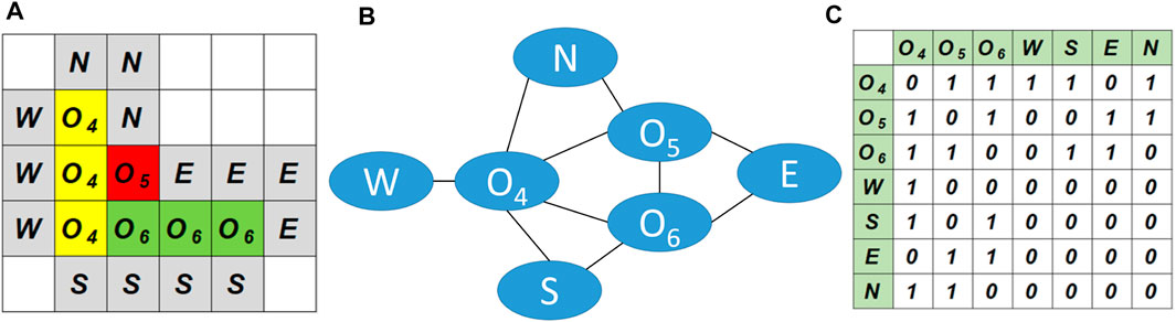
FIGURE 6. (A): geometry of grouped obstacles, (B): obstacles’ adjacency relationship, (C): adjacency matrix.

In general, for a group with n_g obstacles, the size of its adjacency matrix is (n_g + 4) × (n_g + 4), where A_d(i, j) = 1 indicates elements i and j share a borderline. According to the adjacency matrix, new feasible paths are determined in the next step to overcome grouped obstacles. By permutation of the grouped obstacle indices and their surrounding areas that are adjacent to each other, all feasible paths approaching and departing the grouped obstacles from one surrounding area to the other, as well as the path segments on top of the obstacles, can be determined. Similar to the cost value computation for the path segment in Section 3.1, the cost value is assigned to each segment of the newly generated paths. Then, the one with the minimum combined cost is selected for a specific jumping rover to travel over the grouped obstacles.

3.3 Optimal Visiting Sequences

When all feasible routes with and without jumping options are generated between any two targets using the methods described in Sections 3.1, 3.2, a customized GA is applied to search for the optimal sequences to visit all the target points, as well as the charging station when it is necessary. Three parts of the chromosome are included in the customized GA. In Figure 7, the first part represents the target visiting sequences for all UGVs, denoted as [V₁(1), …, V₁ (n₁), V₂ (1), …, V₂(n₂), …, V_p(1), …, V_p(n_p)]. The charging sequences for each UGV are involved in the second part of the chromosome in Figure 7. Associated with each element in the set of V_z, a binary variable is assigned and set as one if a corresponding UGV goes to the charging station after visiting a specific target point, otherwise it is set as zero. Thus, the number of chromosomes in the second part is the same as the length of the first part. The third part of the chromosome represents the number of targets visited by each vehicle, denoted as [n₁, n₂, …, n_p] with ${\sum }_{z=1}^p{n}_z=m+2p-2$. For example, according to the chromosome in Figure 7, the target visiting sequences of UGV 1 is 1-3-2-4-5, and it will be charged after visiting target 2 and then continue to visit target 4 after charging. Then, the overall visiting sequences for UGV 1 is 1-3-2-S-4-5.

FIGURE 7

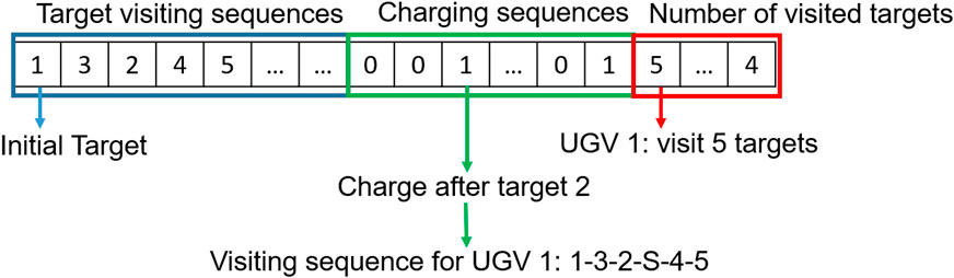
FIGURE 7. Chromosome representation for the UGV team with visiting and charging sequences.

From the initial population, the tournament selection picks a random subset of the population and then chooses the best-fitted chromosome in the selected population set. Among the selected population, the crossover and mutation process will be applied based on the probability of the process. The crossover process only affects the first part of the chromosome, indicating each UGV’s target visiting sequences. We introduce an ordered crossover rather than using a single or two-point crossover to avoid generating invalid solutions. Its child is generated by copying a random number of successive genes and its position from one parent. The remaining genes are implanted in the order of another parent. Then, the mutation process will affect the first and third parts by swapping one gen with another. These operations prevent the genes from being trapped in a local solution.

When generating offspring for the next generation, energy constraints and collisions between rovers are examined. Only collision-free offspring satisfying the energy constraints are chosen for the GA operations described above. Specifically, to satisfy the energy constraint, formulation in Eq. 14 is examined based on the new sequences including the charging sequences. Any chromosome that violates the energy constraint is abandoned and the process is repeated until the sequence satisfies the energy constraints. Next, we examine the collision-free constraints between any two rovers. From RRT, we can obtain time costs as well as energy costs when traveling between two targets. By examining a sequence from GA, we can determine whether one path intersects with another or if there are multiple paths within a rover’s width. If those conflicting paths are assigned to any rovers, the time for corresponding UGVs at the intersection point is calculated. If there is an intersection in time, new paths will be generated by applying a square shape avoidance zone with the length of the square equals to the rover’s width at the intersection point. We then run the GA again to determine the new sequence. This process is repeated until there is no collision among robots. Finally, the fitness value is calculated for every selected population. The fitness value is set the same as the cost function expressed in Eq. 8. The final solution will be determined if the ratio of the best solution in the selected population exceeds the rate of 97%.

For the GA, the crossover and mutation percentages involved in the evolving operations will affect the cost value. Using different combinations of crossover and mutation percentages ranging from 65% to 95%, and .5%–1%, respectively, we aim to find the best combination leading to fast convergence and an optimal solution. Figure 5C shows that most cases converge to a close-optimal solution. However, optimality is not guaranteed for any combination of crossover and mutation percentages. For example, if a low mutation percentage of .5% is used, its convergence speed is slower than other combinations in Figure 5C, associated with a higher cost value. For the worst-case with the crossover percentage of 95% and the mutation percentage of .5%, Figure 5C shows that the cost cannot be reduced within the first 20 iterations and the cost value is much higher than the optimal one when it converges. Therefore, we choose the mutation percentage of 1% and the crossover percentage of 85% when solving this problem.

The entire path planning and task allocation algorithm is summarized into two steps, as shown in Figure 8. In the first step, the optimized path segments with and without jumping options for each UGV are calculated with the corresponding cost determined according to the UGV’s characteristics. Next, the optimal visiting sequences from the initial target to the final target, as well as to the charging station, are determined using the customized GA.

FIGURE 8

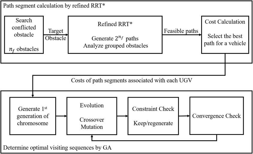
FIGURE 8. Two stages of path planning and task allocation.

4 Simulation and Experiments

4.1 Simulation

To verify the enhanced mobility and energy efficiency of the jumping rover team with a charging station, simulation examples in three scenarios are presented. For Scenario 1, two UGVs are required to visit nine target points without energy constraint, shown in Figures 9A,B. There are seven obstacles, and two of them (O₂ and O₃) have higher elevations that can only be reached by UGV 1 with the jumping option. The two jumping rovers introduced in Section 2 will execute the mission. The characteristics of energy consumption and jumping capability are shown in Table 1, where UGV 1 jumps higher than UGV 2 and consumes about four times as much energy as UGV 2 for every jump.

FIGURE 9

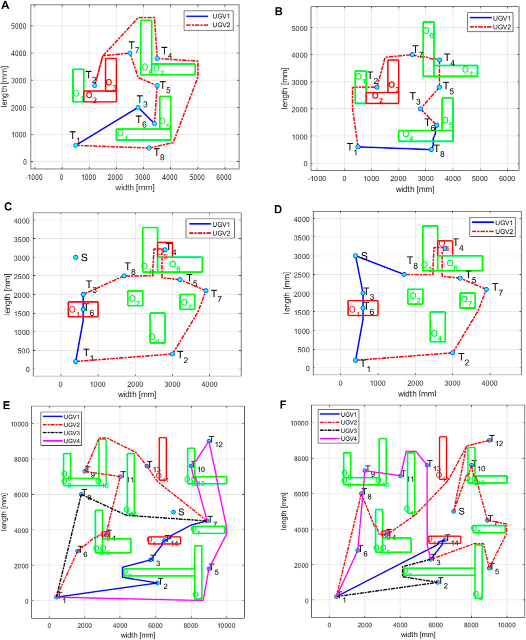
FIGURE 9. Path planning and target allocation simulation (A): without jumping option for scenario 1, (B): with jumping option for scenario 1 (C): without energy constraint for scenario 2, (D): with energy constraint for scenario 2 (E): without energy constraint for scenario 3, (F): with energy constraint for scenario 3

In Scenario 1, we verify the improved energy efficiency and mobility by the UGVs’ jumping capability, where the charging station is not considered. Figure 9A demonstrates the path planning and target allocation results without the jumping option, while Figure 9B shows the corresponding results with the jumping option. With the jumping option, the UGVs choose to jump over some obstacles instead of navigating around the obstacle to visit some targets in Figure 9B. As shown in Table 2, the jumping option leads to reduced energy consumption by about 18% and the byproduct is the reduced mission time around 71%.

TABLE 2

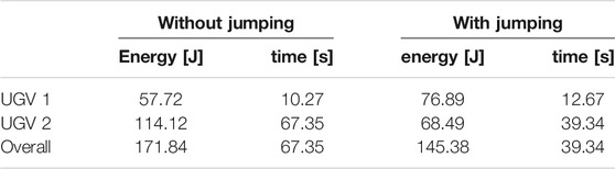
TABLE 2. Comparative results of energy consumption and mission time with and without jumping option in Scenario 1.

In Scenario 2, we seek to verify the improved mission duration via the charging station when considering the energy constraint of each UGV. The jumping option is considered in Scenario 2 and some of the targets are placed on top of the obstacles. Without the energy limitation, the two UGVs’ visiting sequences are (1, 6, 3) for UGV 1 and (1, 2, 7, 5, 4, 8, 3) for UGV 2, as shown in Figure 9C. Their overall energy consumption is 113.44 J (UGV 1: 47.20 J, UGV 2: 66.24 J). When considering the energy constraint (65 J) for each UGV, their visiting sequences are (1, 6, 3, S, 8) for UGV 1 and (1, 2, 7, 5, 4, 8) for UGV 2, as shown in Figure 9D. The overall energy consumption is 78.62 + 65 J (UGV 1: 19.70 + 65 J, UGV 2: 58.92 J), where 65 J is supplied by the charging station for UGV 1. The path segments before traveling to the charging station for the two scenarios are the same. Due to the energy constraint, UGV 2 ends its mission at target 8, and UGV 1 extends its duration by charging its battery after visiting target 3.

In Scenario 3, an extended area including 14 targets and four rovers is considered. We also pursue an enhanced mission duration under energy consumption constraint, where each UGV’s battery capacity is 140 J. UGV 3 is identical to UGV 1 used in Scenario 1, and UGV 4 is the same as UGV 2 used in Scenario 1, in terms of performance features and power consumption characteristics. Without the battery capacity constraint, the visiting sequences of the robot team are (1, 2, 3, 14, 7) for UGV 1, (1, 6, 4, 11, 9, 13, 7) for UGV 2, (1, 8, 7) for UGV3, and (1, 5, 12, 10, 7) for UGV 4, where the planned path for each UGV is shown in Figure 9E. Their overall net energy consumption is about 302 J (UGV 1: 92.04 J, UGV 2: 161.42 J, UGV 3: 68.02 J, UGV 4: 145.48 J). When considering the energy constraints, the visiting sequences of the robot team are (1, 14, 3) for UGV 1, (1, 8, 4, 12, S, 10, 7, 5, 3) for UGV 2, (1, 2, 3) for UGV 3, and (1, 6, 9, 11, 13, 3) for UGV 4, as shown in Figure 9F. Their overall net energy consumption is 270 J (UGV 1: 62.81 J, UGV 2: 30.83 + 140 J, UGV 3: 50.80 J, UGV 4: 126.01 J). To meet the energy constraint, UGV 2 is required to visit the charging station after visiting Target 12 such that it gains extra energy to resume the traveling mission.

4.2 Experiment Verification

The experimental tests are conducted based on Scenario 2 that considers both the jumping option and the energy constraint. As shown in Figure 10A, the charging station provides two outlets that can simultaneously charge two different UGVs. We use the Vicon motion capture system to track the motion of UGVs when executing the planned mission, as shown in Figure 10B. From the motion capture system, we can measure the position and heading angle of rovers, the direction of the charging station, and the location of charging connectors. Then, we can control the rovers’ heading to follow the calculated paths. Throughout the experimental tests, energy consumption data is recorded at a fixed frequency using the current/voltage sensors.

FIGURE 10

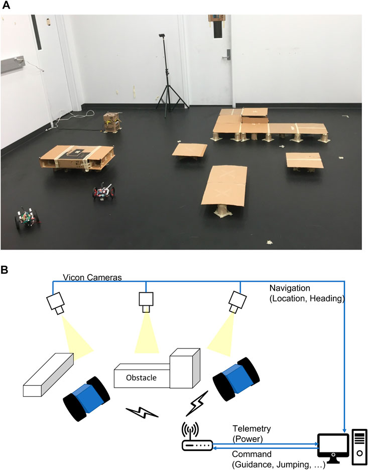
FIGURE 10. Experimental layout and charging station for Scenario 2, (A): mission area, (B): overall experimental configuration.

Figure 11 shows the simulation and experimental results of two UGVs in Scenario 2 using a perspective view. In Table 3, we compare the energy consumption amount in the simulation and experimental results with and without the energy constraint in Scenario 2. The comparison of simulation and experimental data verifies that the experimental results closely match the simulation results. The small differences between the two types of results come from the volume of the charging station, which is approximated as a target point in the simulation. This attributes extra energy consumption in the experiment for the docking motion. Furthermore, the detaching maneuver requires extra energy than nominal driving as the rover needs to overcome the magnetic force that captures the plug.

FIGURE 11

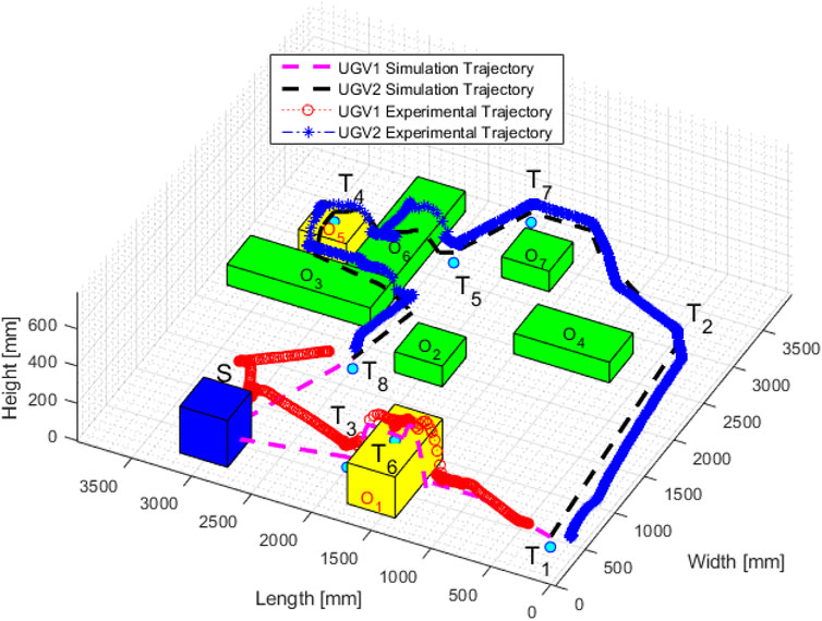
FIGURE 11. Simulation and experimental trajectories of UGVs in Scenario 2 with energy constraint.

TABLE 3

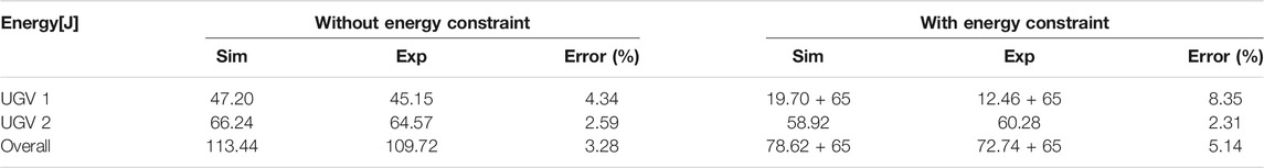
TABLE 3. Energy consumption with and without energy constraint for Scenario 2 in simulation and experimental tests.

In the experimental tests, the two UGVs’ energy consumption at each target point in Scenario 2 without and with the energy constraint is shown in Figures 12A,B, respectively. The total energy consumption without the energy constraint is 109.72 J, and the one with the energy constraint is 72.74 + 65 J, where 65 J is supplied by the charging station. As UGV 1 consumes more energy in both rolling and jumping motion, only three targets are allocated to UGV 1 and the remaining six targets are allocated to UGV 2. Since target 6 is located at the top of an obstacle with a high elevation that can only be reached by UGV 1, UGV 1 visits target 6 and terminates at target 3. When considering the energy constraint, the energy consumption of UGV 1 exceeds the energy constraint after visiting target 3 and it does not have sufficient energy to visit the remaining target points. Different from the case without energy constraint, UGV 2 in this case does not have sufficient energy to visit (1, 2, 7, 5, 4, 8, 3) since visiting these target points consumes 66.24 J, which is larger than the energy constraint, 65 J. Therefore, the charging station extends the UGV mission endurance and thus has the potential to increase the number of targets in an assigned mission area with obstacles. As indicated in Figure 12B, during the battery charging, the actual energy consumption is dropping for UGV 1. Moreover, with a charging station involved in the robot team, it does not require the UGVs to carry heavy batteries, which makes the vehicles lighter. A video file is included as Supplementary Material for the experimental test.

FIGURE 12

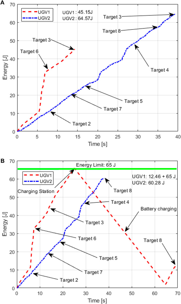
FIGURE 12. Energy consumption at each target point in Scenario 2 (A): without energy constraint, (B): with energy constraint.

5 Conclusion

This paper presents a path planning and task allocation method for a multi-waypoints visiting mission using a group of unmanned ground vehicles with jumping capability and a charging station. The goal is to search for energy-efficient routes to explore a mission area with obstacles. A refined RRT∗ method and a customized genetic algorithm are developed to determine the energy-efficient path and visiting sequences to the assigned targets points and the charging station. The simulation and experimental results verify the advantages of jumping options and the involvement of a charging station in terms of improved mobility, energy efficiency, and extended duration. Future studies will consider more complicated obstacle geometries and investigate the mechanism of controllable jumping height.

Data Availability Statement

The raw data supporting the conclusions of this article will be made available by the authors, without undue reservation.

Author Contributions

MJ developed the path planning and task allocation algorithm, simulated virtual examples, constructed and conducted the experimental tests, and wrote the original manuscript. KT programmed the RRT∗ algorithm and built one of the jumping rovers. RD initiated the jumping rover team concept, refined the algorithm, and revised the manuscript. All authors contributed to this article.

Funding

This work was supported in part by NSF grants ECCS-1815 930.

Conflict of Interest

The authors declare that the research was conducted in the absence of any commercial or financial relationships that could be construed as a potential conflict of interest.

Publisher’s Note

All claims expressed in this article are solely those of the authors and do not necessarily represent those of their affiliated organizations, or those of the publisher, the editors and the reviewers. Any product that may be evaluated in this article, or claim that may be made by its manufacturer, is not guaranteed or endorsed by the publisher.

Supplementary Material

The Supplementary Material for this article can be found online at: https://www.frontiersin.org/articles/10.3389/fcteg.2022.803468/full#supplementary-material

References

Abousleiman, R., Rawashdeh, O., and Boimer, R. (2017). Electric Vehicles Energy Efficient Routing Using Ant colony Optimization. SAE Int. J. Alt. Power 6, 1–14. doi:10.4271/2017-01-9075

CrossRef Full Text | Google Scholar

Archetti, C., Speranza, M. G., and Hertz, A. (2006). A Tabu Search Algorithm for the Split Delivery Vehicle Routing Problem. Transportation Sci. 40, 64–73. doi:10.1287/trsc.1040.0103

CrossRef Full Text | Google Scholar

Barzegaran, M. R., Zargarzadeh, H., and Mohammed, O. A. (2017). Wireless Power Transfer for Electric Vehicle Using an Adaptive Robot. IEEE Trans. Magn. 53, 1–4. doi:10.1109/tmag.2017.2664800

CrossRef Full Text | Google Scholar

Behl, M., DuBro, J., Flynt, T., Hameed, I., Lang, G., and Park, F. (2019). “Autonomous Electric Vehicle Charging System,” in 2019 Systems and information engineering design symposium (SIEDS) (IEEE), 1–6. doi:10.1109/sieds.2019.8735620

CrossRef Full Text | Google Scholar

Belmecheri, F., Prins, C., Yalaoui, F., and Amodeo, L. (2013). Particle Swarm Optimization Algorithm for a Vehicle Routing Problem with Heterogeneous Fleet, Mixed Backhauls, and Time Windows. J. Intell. Manuf 24, 775–789. doi:10.1007/s10845-012-0627-8

CrossRef Full Text | Google Scholar

Chen, D., Bai, F., and Wu, L. (2008). “Kinematics Control of Wheeled Robot Based on Angular Rate Sensors,” in 2008 IEEE Conference on Robotics, Automation and Mechatronics (IEEE), 598–602. doi:10.1109/ramech.2008.4690885

CrossRef Full Text | Google Scholar

Ding, Y., and Park, H.-W. (2017). “Design and Experimental Implementation of a Quasi-Direct-Drive Leg for Optimized Jumping,” in 2017 IEEE/RSJ International Conference on Intelligent Robots and Systems (IROS) (IEEE), 300–305. doi:10.1109/iros.2017.8202172

CrossRef Full Text | Google Scholar

Hockman, B., and Pavone, M. (2020). “Stochastic Motion Planning for Hopping Rovers on Small Solar System Bodies,” in Robotics Research (Springer), 877–893. doi:10.1007/978-3-030-28619-4_60

CrossRef Full Text | Google Scholar

Ichihara, Y., and Ohnishi, K. (2006). “Path Planning and Tracking Control of Wheeled mobile Robot Considering Robots Capacity,” in 2006 IEEE International Conference on Industrial Technology (IEEE), 176–181. doi:10.1109/icit.2006.372372

CrossRef Full Text | Google Scholar

Iwamoto, N., and Yamamoto, M. (2015). “Jumping Motion Control Planning for 4-wheeled Robot with a Tail,” in IEEE/SICE International Symposium on System Integration (SII), 871–876. doi:10.1109/sii.2015.7405114

CrossRef Full Text | Google Scholar

Karaman, S., Walter, M. R., Perez, A., Frazzoli, E., and Teller, S. (2011). “Anytime Motion Planning Using the Rrt,” in IEEE International Conference on Robotics and Automation, 1478–1483. doi:10.1109/icra.2011.5980479

CrossRef Full Text | Google Scholar

Kavraki, L. E., Svestka, P., Latombe, J.-C., and Overmars, M. H. (1996). Probabilistic Roadmaps for Path Planning in High-Dimensional Configuration Spaces. IEEE Trans. Robot. Automat. 12, 566–580. doi:10.1109/70.508439

CrossRef Full Text | Google Scholar

Kingry, N., Liu, Y.-C., Martinez, M., Simon, B., Bang, Y., and Dai, R. (2017). “Mission Planning for a Multi-Robot Team with a Solar-Powered Charging Station,” in IEEE/RSJ International Conference on Intelligent Robots and Systems (IROS), 5233–5238. doi:10.1109/iros.2017.8206413

CrossRef Full Text | Google Scholar

Kok, A. L., Hans, E. W., Schutten, J. M. J., and Zijm, W. H. M. (2010). A Dynamic Programming Heuristic for Vehicle Routing with Time-dependent Travel Times and Required Breaks. Flex Serv. Manuf J. 22, 83–108. doi:10.1007/s10696-011-9077-4

CrossRef Full Text | Google Scholar

LaValle, S. M., and Kuffner, J. J. (2001). Randomized Kinodynamic Planning. Int. J. robotics Res. 20, 378–400. doi:10.1177/02783640122067453

CrossRef Full Text | Google Scholar

LaValle, S. (1998). “Rapidly-exploring Random Trees: a New Tool for Path Planning,” in The Annual Research Report.

Google Scholar

Mathew, N., Smith, S. L., and Waslander, S. L. (2015). Multirobot Rendezvous Planning for Recharging in Persistent Tasks. IEEE Trans. Robot. 31, 128–142. doi:10.1109/tro.2014.2380593

CrossRef Full Text | Google Scholar

Michaud, F., and Robichaud, E. (2002). “Sharing Charging Stations for Long-Term Activity of Autonomous Robots,” in IEEE/RSJ International Conference on Intelligent Robots and Systems, 3, 2746–2751.

Google Scholar

Mizumura, Y., Ishibashi, K., Yamada, S., Takanishi, A., and Ishii, H. (2017). “Mechanical Design of a Jumping and Rolling Spherical Robot for Children with Developmental Disorders,” in IEEE International Conference on Robotics and Biomimetics (ROBIO), 1062–1067. doi:10.1109/robio.2017.8324558

CrossRef Full Text | Google Scholar

Morad, S., Kalita, H., and Thangavelautham, J. (2018). “Planning and Navigation of Climbing Robots in Low-Gravity Environments,” in 2018 IEEE/ION Position, Location and Navigation Symposium (PLANS), 1302–1310. doi:10.1109/plans.2018.8373520

CrossRef Full Text | Google Scholar

Ou, W., and Sun, B.-G. (2010). “A Dynamic Programming Algorithm for Vehicle Routing Problems,” in International Conference on Computational and Information Sciences, 733–736. doi:10.1109/iccis.2010.182

CrossRef Full Text | Google Scholar

Parrot, S. A. (2019). Parrot Jumping Sumo-Races, Slaloms, Acrobatics, You Can Do It All. Available at: https://www.parrot.com/us/minidrones/parrot-jumping-sumo (Accessed August 20, 2019).

Pettie, S., and Ramachandran, V. (2002). An Optimal Minimum Spanning Tree Algorithm. J. Acm 49, 16–34. doi:10.1145/505241.505243

CrossRef Full Text | Google Scholar

Tan, K. C., Jung, M., and Dai, R. (2020). “Motion Planning and Task Allocation for a Jumping Rover Team,” in IEEE/RSJ International Conference on Robotics and Automation (ICRA). doi:10.1109/icra40945.2020.9197268

CrossRef Full Text | Google Scholar

Ushijima, M., Kunii, Y., Maeda, T., Yoshimitsu, T., and Otsuki, M. (2017). “Path Planning with Risk Consideration on Hopping Mobility,” in IEEE/SICE International Symposium on System Integration (SII), 692–697. doi:10.1109/sii.2017.8279302

CrossRef Full Text | Google Scholar

Ye, C., Wang, B., Wei, B., and Tang, B. (2018). “Modeling and Analysis of a Jumping Robot with Deforming Wheeled Mechanism,” in IEEE International Conference on Mechatronics and Automation (ICMA), 980–985. doi:10.1109/icma.2018.8484395

CrossRef Full Text | Google Scholar