Conversion From Unstructured LTI Controllers to Observer-Structured Ones for LPV Systems

1 Introduction

It is well-known that H_∞ control is a powerful tool for controlling plant systems with uncertainties (Zhou et al., 1996). At first, the Riccati equation–based synthesis approach is proposed (Doyle et al., 1989); however, the plant systems should satisfy several assumptions (the so-called “standard assumption”), and this restriction diminishes their applicability and usability. On this issue, after the paper by Sampei et al. (1990) which tackles H_∞ controller synthesis with output feedback controllers in terms of linear matrix inequality (LMI), many research studies on LMI-based H_∞ controller synthesis have been conducted (Gahinet and Apkarian, 1994; Iwasaki and Skelton, 1994; Masubuchi et al., 1998), and the applicability and usability of H_∞ control have been extended. However, it is also well-known that H_∞ controllers have a complicated structure; that is, H_∞ controllers have no special structures as H₂ controllers whose structure is composed of LQR controllers and observers. Due to this property, on-site engineers have a difficulty to understand the structure of H_∞ controllers as well as the meaning of the figures of the state-space matrices of the designed H_∞ controllers.

On this issue, Alazard has explored a new horizon in the studies of Alazard and Apkarian (1999) and Alazard (2012). In the study by Alazard and Apkarian (1999), for LTI plant systems with no direct feedthrough, the authors have proposed a conversion method from a priori designed unstructured LTI controllers to Luenberger observer–based LTI controllers by finding appropriate state transformation matrices for the controllers. Furthermore, in the study of Alazard (2012), the method in the study of Alazard and Apkarian (1999) is extended to the case in which a direct feedthrough exists. In those papers, the dimensions of the controllers are not restricted to be the same as those of the plant systems; that is, even if the dimensions of the controllers are different from those of the plant systems, appropriate state transformation matrices which render the unstructured LTI controllers to Luenberger observer–based controllers can be found by solving the generalized non-symmetric and rectangular Riccati equation. In summary, LTI controllers (including H_∞ controllers) for LTI plant systems can be equivalently represented as Luenberger observer–based controllers using the methods in those papers. This achievement is very helpful for on-site engineers because a priori designed unstructured LTI controllers can be converted to well-known Luenberger observer–based controllers without deteriorating control performance as long as the plant systems are LTI systems. As an application example, the converted controllers can be used as “virtual sensors” (Goupil et al., 2014) for plant health monitoring, fault detection, etc., without any additional controllers or observers because the state of the converted controllers, i.e., Luenberger observer–based controllers, estimates the plant state faithfully. Some application examples can be found in the study of Alazard (2012). By considering the above, it is concluded that the conversion from unstructured LTI controllers to observer-based controllers is useful.

Although the methods in the studies of Alazard and Apkarian (1999) and Alazard (2012) are effective and attractive, there is a drawback that the methods cannot be applied to plant systems which are given as linear parameter-varying (LPV) systems. This is because Luenberger observer–based controllers need the nominal state-space matrices of the plant systems; however, as demonstrated by Peaucelle et al. (2017), Sato (2018), etc., the use of the nominal state-space matrices of plant systems does not always lead to the optimal H_∞ control performance. This fact poses a simple question: “Under the supposition that LPV plant systems can be interpreted to be composed of their nominal LTI plant systems and norm bounded variations, do the methods in the studies of Alazard and Apkarian (1999) and Alazard (2012) give the state transformation matrices which minimize the discrepancies between plant systems’ state and converted controllers’ state even for LPV plant systems?” This question motivates us to try to extend the methods in the studies of Alazard and Apkarian (1999) and Alazard (2012) to the case in which the plant systems are given as LPV systems, and also to try to find the counterpart conversion method for LPV plant systems. That is, our addressed problem in this paper is the counterpart problem in the studies of Alazard and Apkarian (1999) and Alazard (2012) for LPV plant systems. To this end, we first propose observer-structured LTI controllers whose structure is similar to but not exactly the same as the so-called Luenberger observer–based controllers. By using the observer-structured controllers, we then propose a method producing appropriate state transformation matrices which convert the a priori designed unstructured LTI controllers to observer-structured LTI controllers. As a consequence, even if plant systems are given as LPV systems, we can use the converted controllers obtained by our proposed method as “virtual sensors” (Goupil et al., 2014) for plant health monitoring, fault detection, etc., without any additional controllers or observers.

This paper is structured as follows: In Section 2, we first give definitions of an LPV plant system with a direct feedthrough and strictly proper LTI controllers (an unstructured controller designed a priori and an observer-structured controller), then show our parameterization of the observer-structured controller with the state-space matrices of the unstructured controller, one free matrix and a state transformation matrix, and finally clarify the relation between our method and the method in the study of Alazard (2012) for the case that plant systems are given as LTI systems with direct feedthrough, and the dimensions of the controllers are the same as those of the LTI plant systems. In Section 3, we propose a method to obtain the optimal state transformation matrix, which gives the minimum convergence of the discrepancy between the plant state and the observer-structured controller state for a stochastically defined non-zero initial plant state, in terms of parameter-dependent linear matrix inequality (LMI). In Section 4, several toy examples are introduced to illustrate our contributions (i.e., proposition and parameterization of observer-structured controllers, and proposition of design method for state transformation matrices minimizing the estimation errors), and finally, we give concluding remarks in Section 5.

We summarize the notation used in this paper. $\mathbf{0}$ and I_n, respectively, denote a compatibly dimensional zero matrix and an n × n identity matrix; ${\mathbb{R}}^n$, ${\mathbb{R}}^{n\times m}$, and ${\mathbb{S}}_{+}^n$, respectively, denote the sets of n-dimensional real vectors, n × m real matrices, and n × n positive-definite real matrices; $\mathsf{H}\mathsf{e}\left\{X\right\}$ is a shorthand notation of X + X^T for a square matrix X; “$\mathsf{s}\mathsf{y}\mathsf{m}$” in a matrix denotes an abbreviated element by its symmetry; for a square matrix X, $\mathsf{T}\mathsf{r}\left(X\right)$ denotes its trace. In this paper, we address the continuous-time (CT) case as well as the discrete-time (DT) case simultaneously; therefore, the operator δ [⋅] is used to denote the time-derivative in the CT case and one-step shift operator in the DT case. That is, δ [x] in the CT case denotes $\frac{\mathrm{d}}{\mathrm{d}\mathrm{t}}x(t)$ for the current time t, and δ [x] in the DT case denotes x(k + 1) for the current step number k. Similarly, Φ in inequalities denotes $\left[\begin{array}{cc}\hfill \delta [\cdot ]\hfill & \hfill 1\hfill \\ \hfill 1\hfill & \hfill 0\hfill \end{array}\right]$ for the CT case and $\left[\begin{array}{cc}\hfill -1\hfill & \hfill 0\hfill \\ \hfill 0\hfill & \hfill \delta [\cdot ]\hfill \end{array}\right]$ for the DT case.

2 Proposed Parameterization

2.1 Linear Parameter-Varying Plant System

Let us suppose that the stabilization problem of the following LPV plant system is addressed:

$G\left(\theta \right):\left[\begin{array}{c}\hfill \delta \left[x\right]\hfill \\ \hfill y\hfill \end{array}\right]=\left[\begin{array}{cc}\hfill A\left(\theta \right)\hfill & \hfill B\left(\theta \right)\hfill \\ \hfill C\left(\theta \right)\hfill & \hfill D\left(\theta \right)\hfill \end{array}\right]\left[\begin{array}{c}\hfill x\hfill \\ \hfill u\hfill \end{array}\right],(1)$

where $x\in {\mathbb{R}}^n$ denotes the state, $y\in {\mathbb{R}}^{n_y}$ denotes the measurement output, $u\in {\mathbb{R}}^{n_u}$ denotes the control input, and matrices A(θ), B(θ), C(θ), and D(θ) are supposed to be compatibly dimensional real matrices which are dependent on parameters $\theta ={\left[{\theta }_1,\dots ,{\theta }_l\right]}^T$. The parameters can be scheduling parameters as well as uncertainty parameters. Here, it is supposed that all parameters are independent from each other. It is also supposed that the existing regions of parameters and their derivatives (CT case) or deviations per single sampling period (DT case) are bounded. Thus, the following are supposed with a priori given polytopes Λ_i:

$\left({\theta }_i,\delta \left[{\theta }_i\right]\right)\in {\mathrm{\Lambda }}_i,\left(i=1,\dots l\right).(2)$

Then, the following is also supposed:

$\left(\theta ,\delta \left[\theta \right]\right)\in \mathrm{\Lambda }≔{\mathrm{\Lambda }}_1\times \cdots \times {\mathrm{\Lambda }}_l.(3)$

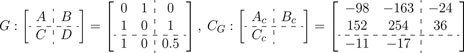
2.2 Unstructured Linear Time-Invariant Controller

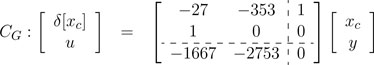
We next define an unstructured LTI controller which has already been designed:

$C_G:\left[\begin{array}{c}\hfill \delta \left[x_c\right]\hfill \\ \hfill u\hfill \end{array}\right]=\left[\begin{array}{cc}\hfill A_c\hfill & \hfill B_c\hfill \\ \hfill C_c\hfill & \hfill \mathbf{0}\hfill \end{array}\right]\left[\begin{array}{c}\hfill x_c\hfill \\ \hfill y\hfill \end{array}\right],(4)$

where $x_c\in {\mathbb{R}}^{n_c}$ denotes the state, and matrices $A_c\in {\mathbb{R}}^{n_c\times n_c}$, $B_c\in {\mathbb{R}}^{n_c\times n_y}$ and $C_c\in {\mathbb{R}}^{n_u\times n_c}$ are constant matrices. Note that the dimension of the controller, i.e., n_c, might be different from that of the plant system; that is, it can be possible that n_c ≠ n holds in our proposed parameterization.

Then, the closed-loop system comprising G(θ) and C_G is straightforwardly derived as follows:

$G_{cl}^G\left(\theta \right):\left[\begin{array}{c}\hfill \delta \left[x\right]\hfill \\ \hfill \delta \left[x_c\right]\hfill \end{array}\right]=\underset{A_{cl}^G\left(\theta \right)}{\underbrace{\left[\begin{array}{cc}\hfill A\left(\theta \right)\hfill & \hfill B\left(\theta \right)C_c\hfill \\ \hfill B_{c}C\left(\theta \right)\hfill & \hfill A_c+B_{c}D\left(\theta \right)C_c\hfill \end{array}\right]}}\left[\begin{array}{c}\hfill x\hfill \\ \hfill x_c\hfill \end{array}\right].(5)$

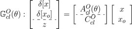
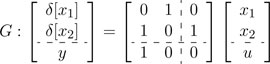
2.3 Observer-Structured Linear Time-Invariant Controller

We next define an observer-structured LTI controller inspired by Sato (2020a). In the DT case, only predictor form (Alazard, 2012) is considered hereafter:

$C_O:\left\{\begin{array}{ccc}\hfill \delta \left[x_o\right]\hfill & \hfill =\hfill & A_o{x}_o+B_{o}u-L\left(y-C_o{x}_o-D_{o}u\right),\hfill \\ \hfill u\hfill & \hfill =\hfill & K{x}_o,\hfill \end{array}\right.(6)$

where $x_o\in {\mathbb{R}}^{n_c}$ denotes the state, and not only matrices $L\in {\mathbb{R}}^{n_c\times n_y},K\in {\mathbb{R}}^{n_u\times n_c}$ but also matrices $A_o\in {\mathbb{R}}^{n_c\times n_c},B_o\in {\mathbb{R}}^{n_c\times n_u},C_o\in {\mathbb{R}}^{n_y\times n_c}$, $D_o\in {\mathbb{R}}^{n_y\times n_u}$ are to be determined.

Then, the closed-loop system comprising G(θ) and C_O is straightforwardly derived as follows:

$G_{cl}^O\left(\theta \right):\left[\begin{array}{c}\hfill \delta \left[x\right]\hfill \\ \hfill \delta \left[x_o\right]\hfill \end{array}\right]=\underset{A_{cl}^O\left(\theta \right)}{\underbrace{\left[\begin{array}{cc}\hfill A\left(\theta \right)\hfill & \hfill B\left(\theta \right)K\hfill \\ \hfill -LC\left(\theta \right)\hfill & \hfill A_o+B_{o}K+L{C}_o-L\left(D\left(\theta \right)-D_o\right)K\hfill \end{array}\right]}}\left[\begin{array}{c}\hfill x\hfill \\ \hfill x_o\hfill \end{array}\right].(7)$

Remark 1. As is obvious, the controller $C_O$ does not have the same structure as the so-called “Luenberger observer–based controller” does. However, if there are no parameters in the LPV plant system, that is, the LTI plant system $G$ is supposed instead of the LPV plant system $G(\theta )$, then setting $A_o$, $B_o$, $C_o$, and $D_o$ to be $A$, $B$, $C$, and $D$, respectively, makes the controller $C_O$ to be identical to the conventional “Luenberger observer–based controller.” Therefore, the controller $C_O$ is referred to as the observer-structured controller due to the structural similarity between the observer-structured controller $C_O$ and the “Luenberger observer–based controller.”

2.4 Parameterization of Observer-Structured Linear Time-Invariant Controller

By comparing $G_{cl}^G(\theta )$ and $G_{cl}^O(\theta )$ under the consideration of the freedom of the state transformation x_o = T⁻¹x_c with a non-singular matrix T, it is easily confirmed that the two systems are equivalent if the following equations hold:

$\left\{\begin{array}{c}KT{}^{-1}=C_c,\hfill \\ -TL=B_c,\hfill \\ T\left(A_o+B_{o}K+L{C}_o+L{D}_{o}K\right)T^{-1}=A_c.\hfill \end{array}\right.(8)$

The last equation in Eq. 8 is equivalently represented as follows:

$\underset{Y_B}{\underbrace{\left[\begin{array}{cc}\hfill {\mathbf{I}}_{n_c}\hfill & \hfill -B_c\hfill \end{array}\right]}}\underset{X_O}{\underbrace{\left[\begin{array}{cc}\hfill T{A}_{o}T{}^{-1}\hfill & \hfill T{B}_o\hfill \\ \hfill C_o{T}^{-1}\hfill & \hfill D_o\hfill \end{array}\right]}}\underset{Y_C}{\underbrace{\left[\begin{array}{c}\hfill {\mathbf{I}}_{n_c}\hfill \\ \hfill C_c\hfill \end{array}\right]}}=A_c.(9)$

Then, we give one of our main results.

Theorem 1. The matrix $X_O\in {\mathbb{R}}^{(n_c+n_y)\times (n_c+n_u)}$ satisfying Eq. 9 is parameterized as in Eq. 10 with one free matrix $Z\left(\theta \right)\in {\mathbb{R}}^{(n_c+n_y)\times (n_c+n_u)}$:

$X_O=Y_B^{†}{A}_c{Y}_C^{†}+Z\left(\theta \right)-Y_B^{†}{Y}_{B}Z\left(\theta \right)Y_C{Y}_C^{†},(10)$

where matrices with superscript “^†” denote the corresponding Moore–Penrose inverse matrices.

Proof 1. The corresponding assertion for constant matrices is easily proved by using Theorem 2.3.1 in the study of Skelton et al. (1998), and thus, our claim is also easily proved. However, for completeness, we give the detailed proof.We now prove that the following two statements are equivalent:

1) There exists a solution satisfying Eq. 9, and all the solutions are parameterized as in Eq. 10.

2) $Y_B{Y}_B^{†}{A}_c{Y}_C^{†}{Y}_C=A_c$

We first prove that 2) holds when 1) holds. Multiplying $Y_B{Y}_B^{†}$ and $Y_C^{†}{Y}_C$ to both the sides of Eq. 9 from the left and the right, respectively, leads to $Y_B{Y}_B^{†}{Y}_B{X}_O{Y}_C{Y}_C^{†}{Y}_C\left(=Y_B{X}_O{Y}_C\right)=Y_B{Y}_B^{†}{A}_c{Y}_C^{†}{Y}_C$. From Eq. 9, Y_BX_OY_C is obviously identical to A_c. Thus, 1) ⇒ 2) is proved.Next, we prove that 1) holds when 2) holds. To this end, we first confirm that X_O in Eq. 10 is the solution of Eq. 9. Multiplying Y_B and Y_C to the left-hand side of Eq. 10 from the left and the right, respectively, leads to Y_BX_OY_C. The same manipulation to the right-hand side of Eq. 10 leads to $Y_B{Y}_B^{†}{A}_c{Y}_C^{†}{Y}_C+Y_{B}Z(\theta )Y_C-Y_B{Y}_B^{†}{Y}_{B}Z(\theta )Y_C{Y}_C^{†}{Y}_C$, which is equivalent to $Y_B{Y}_B^{†}{A}_c{Y}_C^{†}{Y}_C$. Thus, when 2) holds, $Y_B{X}_O{Y}_C(=Y_B{Y}_B^{†}{A}_c{Y}_C^{†}{Y}_C)=A_c$ is derived; then, it is confirmed that X_O in Eq. 10 is the solution of Eq. 9.We finally confirm that all solutions of Eq. 9 are parameterized as X_O as in Eq. 10. To this end, we replace A_c in Eq. 10 by the left-hand side of Eq. 9, and then the following is derived:

$X_O=Y_B^{†}{Y}_B{X}_O{Y}_C{Y}_C^{†}+Z\left(\theta \right)-Y_B^{†}{Y}_{B}Z\left(\theta \right)Y_C^{†}{Y}_C^{†}.$

This equation always holds as long as Z(θ) is set as X_O. Thus, each X_O satisfying Eq. 9 has each corresponding parameterization matrix Z(θ); that is, all solutions of Eq. 9 are parameterized as in Eq. 10. We have thus proved that the two statements, 1) and 2), are equivalent.As it is easily confirmed that 2) holds from Eq. 9, i.e., $Y_B{Y}_B^{†}{A}_c{Y}_C^{†}{Y}_C=Y_B{Y}_B^{†}{Y}_B{X}_O{Y}_C{Y}_C^{†}{Y}_C=Y_B{X}_O{Y}_C=A_c$ holds, the assertion in Theorem 1, i.e., 1), is now proved. $\square$From Eqs 8–10, the following parameterization of the state-space matrices of C_O is straightforwardly derived with the state-space matrices of C_G in Eq. 4, one free matrix Z(θ), and a non-singular state transformation matrix T:

$\left\{\begin{array}{cc}K\hfill & =C_{c}T,\hfill \\ L\hfill & =-T^{-1}{B}_c,\hfill \\ \left[\begin{array}{cc}\hfill A_o\hfill & \hfill B_o\hfill \\ \hfill C_o\hfill & \hfill D_o\hfill \end{array}\right]\hfill & =\left[\begin{array}{cc}\hfill T^{-1}\hfill & \hfill \mathbf{0}\hfill \\ \hfill \mathbf{0}\hfill & \hfill {\mathbf{I}}_{n_y}\hfill \end{array}\right]\left(Y_B^{†}{A}_c{Y}_C^{†}+Z\left(\theta \right)-Y_B^{†}{Y}_{B}Z\left(\theta \right)Y_C{Y}_C^{†}\right)\left[\begin{array}{cc}\hfill T\hfill & \hfill \mathbf{0}\hfill \\ \hfill \mathbf{0}\hfill & \hfill {\mathbf{I}}_{n_u}\hfill \end{array}\right].\hfill \end{array}\right.(11)$

Remark 2. As the left-hand sides and the right-hand sides of all equations in Eq. 11 are, respectively, constant and parameter-dependent, in general, complicated constraints consequently arise for Z(θ). A simple solution to escape from the complicated constraints is to set Z(θ) to be constant, i.e., Z(θ) = Z. This setting reduces the generality; however, it also reduces numerical complexity when obtaining the state-space matrices A_o, B_o, C_o, and D_o in the next section.Note that matrices A_o, B_o, C_o, and D_o have freedom as in the last equation of Eq. 11; however, they must satisfy Eq. 9, i.e., the last equation of Eq. 8. That is, we would like to emphasize that even if they are chosen as desired matrices within the parameterization of Eq. 11, the input–output property of C_O is the same as that of C_G. Therefore, the essential freedom of the conversion from C_G to C_O is only the state transformation represented by T.In the next section, we propose a design method to obtain the optimal state transformation matrix with respect to the convergence of the discrepancy between the plant state and the observer-structured controller state for a stochastically defined non-zero initial plant state, and then we also propose a method to obtain matrices A_o, B_o, C_o, and D_o as close to as the designated matrices within the parameterization of the last equation of Eq. 11.

2.5 Relation Between Our Method and Existing Method for Linear Time-Invariant Plant Systems

In this subsection, we clarify the relation between our method and the method in the study of Alazard (2012) for LTI plant systems. For simplicity, n_c is supposed to be equal to n; that is, only full-order controllers are considered. In the DT case, only predictor form (Alazard, 2012) is considered.

2.5.1 Brief Review of Existing Method in the Study of Alazard (2012)

Now, it is supposed that the plant system is given as an LTI system:

$G:\left[\begin{array}{c}\hfill \delta \left[x\right]\hfill \\ \hfill y\hfill \end{array}\right]=\left[\begin{array}{cc}\hfill A\hfill & \hfill B\hfill \\ \hfill C\hfill & \hfill D\hfill \end{array}\right]\left[\begin{array}{c}\hfill x\hfill \\ \hfill u\hfill \end{array}\right],(12)$

where $x\in {\mathbb{R}}^n$ denotes the state, $y\in {\mathbb{R}}^{n_y}$ denotes the measurement output, $u\in {\mathbb{R}}^{n_u}$ denotes the control input, and matrices A, B, C, and D are supposed to be compatibly dimensional constant matrices.

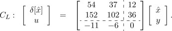
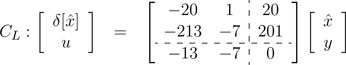
We define the observer-based controller as

$C_L:\left\{\begin{array}{ccc}\hfill \delta \left[\widehat{x}\right]\hfill & \hfill =\hfill & A\widehat{x}+Bu-\mathcal{L}\left(y-C\widehat{x}-Du\right),\hfill \\ \hfill u\hfill & \hfill =\hfill & \mathcal{K}\widehat{x},\hfill \end{array}\right.(13)$

where $\widehat{x}\in {\mathbb{R}}^n$ denotes the observer state and matrices $\mathcal{L}\in {\mathbb{R}}^{n\times n_y}$ and $\mathcal{K}\in {\mathbb{R}}^{n_u\times n}$ are, respectively, the observer gain and the state-feedback gain.

The closed-loop system comprising G and C_L is expressed as follows:

$G_{cl}^L:\left[\begin{array}{c}\hfill \delta \left[x\right]\hfill \\ \hfill \delta \left[\widehat{x}\right]\hfill \end{array}\right]=\underset{A_{cl}^L}{\underbrace{\left[\begin{array}{cc}\hfill A\hfill & \hfill B\mathcal{K}\hfill \\ \hfill -\mathcal{L}C\hfill & \hfill A+B\mathcal{K}+\mathcal{L}C\hfill \end{array}\right]}}\left[\begin{array}{c}\hfill x\hfill \\ \hfill \widehat{x}\hfill \end{array}\right].(14)$

In order to make the closed-loop system $G_{cl}^L$ identical to $G_{cl}^G(\theta )$ in Eq. 5 for an LTI plant system G in Eq. 12, the state transformation $\widehat{x}={\mathcal{T}}^{-1}{x}_c$ with a non-singular matrix $\mathcal{T}\in {\mathbb{R}}^{n\times n}$ is considered. Then, the following conditions are straightforwardly derived:

$\left\{\begin{array}{c}\mathcal{K}=C_c\mathcal{T}\hfill \\ -\mathcal{L}={\mathcal{T}}^{-1}{B}_c\hfill \\ A+B\mathcal{K}+\mathcal{L}C={\mathcal{T}}^{-1}\left(A_c+B_{c}D{C}_c\right)\mathcal{T}\hfill \end{array}\right.(15)$

If an appropriate $\mathcal{T}$ is found, then $\mathcal{K}$ and $\mathcal{L}$ are, respectively, given as $C_c\mathcal{T}$ and $-{\mathcal{T}}^{-1}{B}_c$. Then, the remaining task is to find the state transformation matrix $\mathcal{T}$ satisfying

$\mathcal{T}A+\mathcal{T}B{C}_c\mathcal{T}-B_{c}C=(A_c+B_{c}D{C}_c)\mathcal{T},$

i.e.,

$\left[\begin{array}{cc}\hfill \mathcal{T}\hfill & \hfill -{\mathbf{I}}_n\hfill \end{array}\right]\left[\begin{array}{cc}\hfill A\hfill & \hfill B{C}_c\hfill \\ \hfill B_{c}C\hfill & \hfill A_c+B_{c}D{C}_c\hfill \end{array}\right]\left[\begin{array}{c}\hfill {\mathbf{I}}_n\hfill \\ \hfill \mathcal{T}\hfill \end{array}\right]=\mathbf{0}.(16)$

The solution of Eq. 16 can be obtained by the following method (Alazard, 2012):

• Choose n closed-loop eigenvalues which are the eigenvalues of $A+B\mathcal{K}$.

• Find n-dimensional invariant subspace, i.e., matrices $U_1,U_2\in {\mathbb{R}}^{n\times n}$ such that

$\left[\begin{array}{cc}\hfill A\hfill & \hfill B{C}_c\hfill \\ \hfill B_{c}C\hfill & \hfill A_c+B_{c}D{C}_c\hfill \end{array}\right]\left[\begin{array}{c}\hfill U_1\hfill \\ \hfill U_2\hfill \end{array}\right]=\left[\begin{array}{c}\hfill U_1\hfill \\ \hfill U_2\hfill \end{array}\right]\mathrm{\Lambda },$

where the eigenvalues of $\mathrm{\Lambda }\in {\mathbb{R}}^{n\times n}$ are the selected eigenvalues in the previous step.

• If the matrix U₁ is confirmed to be non-singular, then the state transformation matrix is obtained as $\mathcal{T}=U_2{U}_1^{-1}$.

By following the procedure for obtaining $\mathcal{T}$ shown above, the unstructured controller C_G can be converted to the Luenberger observer–based controller C_L with $\mathcal{K}=C_c\mathcal{T}$ and $\mathcal{L}=-{\mathcal{T}}^{-1}{B}_c$.

2.5.2 Comparison of Our Method With Existing Method

Comparing C_O in Eq. 6 and C_L in Eq. 13 concludes that if matrices A_o, B_o, C_o, and D_o are set as A, B, C, and D, respectively, and gain matrices K and L are also set as $\mathcal{K}$ and $\mathcal{L}$, respectively, then C_O is identical to C_L. That is, the observer-structured controller C_O encompasses the Luenberger observer–based controller C_L.

Furthermore, if the state transformation matrix T is set as $\mathcal{T}$ in the method of Alazard (2012), then the two closed-loop systems, i.e., $G_{cl}^O$ and $G_{cl}^L$, are also identical to each other. Thus, if the observer-based controller C_L can be obtained from the unstructured controller C_G by appropriately defined $\mathcal{T}$, then it is always possible to have the same controller within the expression of observer-structured controller C_O by setting T to be identical to $\mathcal{T}$.

In summary, the observer-structured controller encompasses the expression of Luenberger observer–based controller, and the transformation from C_G to C_O also encompasses the corresponding one from C_G to C_L. Thus, we conclude that the observer-structured controller is a kind of generalization of the Luenberger observer–based controller, and the conversion from C_G to C_O is also a kind of generalization of the one from C_G to C_L.

3 Observer-Structured Controller With Optimal Estimation Error for Non-Zero Initial Plant State

In this section, we give a formulation to obtain the optimal state transformation matrix with respect to the convergence of the discrepancy between the plant state and the observer-structured controller state for a stochastically defined non-zero initial plant state.

We first define performance output to be evaluated. Now, the dimension of the unstructured controller is not always the same as that of the LPV plant system. We thus select n_sl state variables of the LPV plant system to be estimated by the observer-structured controller and set the vector containing them as $x_{sl}$ which is expressed as $x_{sl}=C_{sl}x$ with an appropriately defined constant matrix $C_{sl}\in {\mathbb{R}}^{n_{sl}\times n}$. Similarly, the corresponding vector in the observer-structured controller is defined as $x_{o_{sl}}$ which is expressed as $x_{o_{\mathit{sl}}}=C_{s{l}_o}{x}_o$ with an appropriately defined constant matrix $C_{s{l}_0}\in {\mathbb{R}}^{n_{sl}\times n_c}$.

Then, using $G_{cl}^O(\theta )$, we define the following system with performance output z defined as $x_{sl}-x_{o_{sl}}$:

Here, $C_{cl}^O=\left[\begin{array}{cc}\hfill C_{sl}\hfill & \hfill -C_{s{l}_o}\hfill \end{array}\right]$.

By considering that if x_sl and $x_{o_{sl}}$ are close to each other, then it can be concluded that $x_{o_{sl}}$ of the observer-structured controller C_O plays as a good estimation of x_sl of the LPV system G(θ), and we now define the following problem in which the estimation error between the LPV plant state and the converted controller state is minimized.

Problem 1. For ${\mathbb{G}}_{cl}^O(\theta )$ in Eq. 17, obtain the minimal positive scalar γ and the corresponding non-singular matrix T satisfying

$\left\{\begin{array}{c}{\int }_0^{\infty }{z}^{T}z\mathrm{d}\mathrm{t}<\gamma ,\forall \left(\theta ,\delta \left[\theta \right]\right)\in \mathrm{\Lambda }\left(\mathit{CT}\right),\hfill \\ {\sum }_{k=0}^{\infty }{z}^{T}z<\gamma ,\forall \left(\theta ,\delta \left[\theta \right]\right)\in \mathrm{\Lambda }\left(\mathit{DT}\right).\hfill \end{array}\right.(18)$

Here, it is supposed that the initial plant state x(0) is set as a stochastic variable which satisfies E[x(0)] = 0 and E[x(0) x(0)^T] = I_n and that the initial controller states x_c(0) and x_o(0) are both set as 0.To address this problem, we define the following system which is composed of $G_{cl}^G(\theta )$ with the performance output z defined in ${\mathbb{G}}_{cl}^O(\theta )$:Note that the following hold, since x_o = T⁻¹x_c is applied to $G_{cl}^O(\theta )$ to derive Eq. 8:

$\left\{\begin{array}{c}\left[\begin{array}{cc}\hfill {\mathbf{I}}_n\hfill & \hfill \mathbf{0}\hfill \\ \hfill \mathbf{0}\hfill & \hfill T\hfill \end{array}\right]A_{cl}^O\left(\theta \right)\left[\begin{array}{cc}\hfill {\mathbf{I}}_n\hfill & \hfill \mathbf{0}\hfill \\ \hfill \mathbf{0}\hfill & \hfill T^{-1}\hfill \end{array}\right]=A_{cl}^G\left(\theta \right),\hfill \\ C_{cl}^O\left[\begin{array}{cc}\hfill {\mathbf{I}}_n\hfill & \hfill \mathbf{0}\hfill \\ \hfill \mathbf{0}\hfill & \hfill T^{-1}\hfill \end{array}\right]=C_{cl}^G\left(\theta \right).\hfill \end{array}\right.(20)$

Then, the following theorem is proposed for Problem 1.

Theorem 2. If Eq. 21 is solved affirmatively, then ${\mathbb{G}}_{cl}^O(\theta )$ calculated with $T={\mathcal{T}}^{-1}$ satisfies Eq. 18 with the optimized γ:

$\underset{\gamma ,\mathcal{T}\in {\mathbb{R}}^{n_c\times n_c},\mathcal{P}\left(\theta \right)\in {\mathbb{S}}_{+}^{n+n_c}}{\min }\gamma s.t.\left(\text{22}\right),\left(\text{23}\right),and\left(\text{24}\right),(21)$

$\gamma >\mathsf{T}\mathsf{r}\left(\left[\begin{array}{cc}\hfill {\mathbf{I}}_n\hfill & \hfill \mathbf{0}\hfill \end{array}\right]\mathcal{P}\left(\theta \right)\left[\begin{array}{c}\hfill {\mathbf{I}}_n\hfill \\ \hfill \mathbf{0}\hfill \end{array}\right]\right),\forall \left(\theta ,\delta \left[\theta \right]\right)\in \mathrm{\Lambda },(22)$

$\mathcal{P}\left(\theta \right)\succ \mathbf{0},\forall \left(\theta ,\delta \left[\theta \right]\right)\in \mathrm{\Lambda },(23)$

$\left[\begin{array}{cc}\hfill \left[\begin{array}{cc}\hfill {\mathbf{I}}_{n+n_c}\hfill & \hfill A_{cl}^G{(\theta )}^T\hfill \end{array}\right]\left(\mathrm{\Phi }\otimes \mathcal{P}(\theta )\right)\left[\begin{array}{c}\hfill {\mathbf{I}}_{n+n_c}\hfill \\ \hfill A_{cl}^G(\theta )\hfill \end{array}\right]\hfill & \hfill \mathsf{s}\mathsf{y}\mathsf{m}\hfill \\ \hfill \left[\begin{array}{cc}\hfill C_{sl}\hfill & \hfill -C_{s{l}_o}\mathcal{T}\hfill \end{array}\right]\hfill & \hfill -{\mathbf{I}}_{n_{sl}}\hfill \end{array}\right]\prec 0,\forall (\theta ,\delta [\theta ])\in \mathrm{\Lambda }.(24)$

Proof 2. As the upper-left block of the left-hand side of Eq. 24 is negative-definite, the following are confirmed for all combinations of (θ, δ[θ]) ∈ Λ:

$\left\{\begin{array}{c}\frac{\mathrm{d}}{\mathrm{d}\mathrm{t}}\mathcal{P}\left(\theta \right)+\mathsf{H}\mathsf{e}\left\{\mathcal{P}\left(\theta \right)A_{cl}^G\left(\theta \right)\right\}\prec 0\left(\mathbf{CT}\right),\hfill \\ -\mathcal{P}\left(\theta \right)+A_{cl}^G{\left(\theta \right)}^T\mathcal{P}\left({\theta }^{+}\right)A_{cl}^G\left(\theta \right)\prec 0\left(\mathbf{DT}\right).\hfill \end{array}\right.(25)$

Since the positivity of $\mathcal{P}(\theta )$ is ensured in Eq. 23, the stability of ${\mathbb{G}}_{cl}^G(\theta )$ is confirmed.Note that Eq. 24 is equivalent to the following for all combinations of (θ, δ[θ]) ∈ Λ:

$\left[\begin{array}{cc}\hfill {\mathbf{I}}_{n+n_c}\hfill & \hfill A_{cl}^G{(\theta )}^T\hfill \end{array}\right]\left(\mathrm{\Phi }\otimes \mathcal{P}(\theta )\right)\left[\begin{array}{c}\hfill {\mathbf{I}}_{n+n_c}\hfill \\ \hfill A_{cl}^G(\theta )\hfill \end{array}\right]+\left[\begin{array}{c}\hfill C_{sl}^T\hfill \\ \hfill -{\mathcal{T}}^T{C}_{s{l}_o}^T\hfill \end{array}\right]\left[\begin{array}{cc}\hfill C_{sl}\hfill & \hfill -C_{s{l}_o}\mathcal{T}\hfill \end{array}\right]\prec 0.(26)$

After $T={\mathcal{T}}^{-1}$ is set, multiplying $x_{a_c}^T(≔{\left[\begin{array}{cc}\hfill x^T\hfill & \hfill x_c^T\hfill \end{array}\right]}^T)$ and its transpose to Eq. 26 from the left and the right, respectively, leads to the following inequality for all combinations of (θ, δ[θ]) ∈ Λ:

$\left\{\begin{array}{c}{z}^{T}z+\frac{\mathrm{d}}{\mathrm{d}\mathrm{t}}\left(x_{a_c}^T\mathcal{P}\left(\theta \right)x_{a_c}\right)<0\left(\mathbf{CT}\right),\hfill \\ z^{T}z-x_{a_c}^T\mathcal{P}\left(\theta \right)x_{a_c}+\delta \left[x_{a_c}^T\right]\mathcal{P}\left({\theta }^{+}\right)\delta \left[x_{a_c}\right]<0\left(\mathbf{DT}\right).\hfill \end{array}\right.(27)$

Then, the satisfaction of Eq. 18 is confirmed after consideration of the stability of ${\mathbb{G}}_{cl}^G(\theta )$ and Eq. 22. $\square$

Remark 3. If $\mathcal{T}$ is singular, then a small perturbation to $\mathcal{T}$ is to be conducted to obtain non-singular $\mathcal{T}$, similarly to Masubuchi et al. (1998). In particular, if $C_{s{l}_o}$ is set as a row full-rank rectangular matrix, then $\mathcal{T}$ has freedom, which has no effect on the performance index γ, and thus, there is a possibility to have singular $\mathcal{T}$. In this case, a small perturbation to $\mathcal{T}$ is necessary to obtain non-singular $\mathcal{T}$.In general, inequality Eq. 24 is not parametrically affine; thus, some relaxation methods (e.g., sum-of-squares (Chesi et al., 2003; Parrilo, 2003), Polya’s theorem–based relaxation (de Oliveira and Peres, 2007), and slack-variable approach (Peaucelle and Sato, 2009)) should be applied to be solved numerically. However, such relaxations usually increase the numerical complexity. On this issue, if the state-space matrices of the LPV plant G(θ) are supposed to be multi-affine with respect to parameters (Amato et al., 2005; Peacelle and Ebihara, 2018; Sato, 2020b) and the parameter-dependent decision matrix in Theorem 2, i.e., $\mathcal{P}(\theta )$, is also set as multi-affine with respect to parameters, then the multi-affine property [i.e., Lemma 3 in the study of Sato (2020b)] can be used for Theorem 2 after extended/dilated LMI technique (de Oliveira et al., 1999; Peaucelle et al., 2000; Pipeleers et al., 2009) is applied to maintain the numerical complexity as small as possible while conservatism in solving LMIs is also kept small.To this end, the following assumption is now made.

Assumption 1. All the parameter-dependent state-space matrices of G(θ) in Eq. 1 are supposed to be multi-affine with respect to θ_i; that is, they are represented as follows:

$\mathrm{\Gamma }\left(\theta \right)=\sum \underset{1}{\overset{{\alpha }_1}{\theta }}\dots {\theta }_l^{{\alpha }_l}{\mathrm{\Gamma }}_{{\alpha }_1\dots {\alpha }_l},{\alpha }_i=\left\{\mathrm{0,1}\right\},(28)$

where ${\mathrm{\Gamma }}_{{\alpha }_1\dots {\alpha }_l}$ is the coefficient matrix.Then, the following lemma is straightforwardly derived from Theorem 2 with the use of extended/dilated LMI technique (de Oliveira et al., 1999; Peaucelle et al., 2000; Pipeleers et al., 2009) and multi-affine property [i.e., Lemma 3 in the study of Sato (2020b)].

Lemma 1. Under Assumption 1, if Eq. 29 is solved affirmatively with multi-affine $\mathcal{P}(\theta )$, then ${\mathbb{G}}_{cl}^O(\theta )$ calculated with $T={\mathcal{T}}^{-1}$ (if necessary, a small perturbation in Remark 3 is conducted) satisfies Eq. 18 with the optimized γ:

$\underset{\gamma ,\mathcal{T}\in {\mathbb{R}}^{n_c\times n_c},\mathcal{P}\left(\theta \right)\in {\mathbb{S}}_{+}^{n+n_c},\mathcal{H}\in {\mathbb{R}}^{2\left(n+n_c\right)\times \left(n+n_c\right)}}{\min }\gamma s.t.\left(\text{30}\right),\left(\text{31}\right),and\left(\text{32}\right),(29)$

$\gamma >\mathsf{T}\mathsf{r}\left(\left[\begin{array}{cc}\hfill {\mathbf{I}}_n\hfill & \hfill \mathbf{0}\hfill \end{array}\right]\mathcal{P}\left(\theta \right)\left[\begin{array}{c}\hfill {\mathbf{I}}_n\hfill \\ \hfill \mathbf{0}\hfill \end{array}\right]\right),\forall \left(\theta ,\delta \left[\theta \right]\right)\in \mathsf{v}\mathsf{e}\mathsf{r}\left(\mathrm{\Lambda }\right),(30)$

$\mathcal{P}\left(\theta \right)\succ 0,\forall \left(\theta ,\delta \left[\theta \right]\right)\in \mathsf{v}\mathsf{e}\mathsf{r}\left(\mathrm{\Lambda }\right),(31)$

$\left[\begin{array}{cc}\hfill \left(\begin{array}{c}\hfill \mathsf{H}\mathsf{e}\left\{\mathcal{H}\left[\begin{array}{cc}\hfill A_{cl}^G(\theta )\hfill & \hfill -{\mathbf{I}}_{n+n_c}\hfill \end{array}\right]\right\}\hfill \\ \hfill +{\mathbf{I}}_{2(n+n_c)}\left(\mathrm{\Phi }\otimes \mathcal{P}(\theta )\right){\mathbf{I}}_{2(n+n_c)}\hfill \end{array}\right)\hfill & \hfill \mathsf{s}\mathsf{y}\mathsf{m}\hfill \\ \hfill \left[\begin{array}{cc}\hfill \left[\begin{array}{cc}\hfill C_{sl}\hfill & \hfill -C_{s{l}_o}\mathcal{T}\hfill \end{array}\right]\hfill & \hfill 0\hfill \end{array}\right]\hfill & \hfill -{\mathbf{I}}_{n_{sl}}\hfill \end{array}\right]\prec 0,\forall (\theta ,\delta [\theta ])\in \mathsf{v}\mathsf{e}\mathsf{r}(\mathrm{\Lambda }).(32)$

In inequalities (Eqs 30–32), $\mathsf{v}\mathsf{e}\mathsf{r}\left(\cdot \right)$ denotes the vertex set.The proof is omitted as it is straightforward in consideration of the following relation:

$\left[\begin{array}{cc}\hfill \begin{array}{c}\hfill [{\mathbf{I}}_{n+n_c}{A}_{cl}^G{\left(\theta \right)}^T]\hfill \end{array}\hfill & \hfill \mathbf{0}\hfill \\ \hfill \mathbf{0}\hfill & \hfill {\mathbf{I}}_{n_{sl}}\hfill \end{array}\right]\left(left-handsideof(32)\right)\left[\begin{array}{cc}\hfill \left[\begin{array}{c}\hfill {\mathbf{I}}_{n+n_c}\hfill \\ \hfill A_{cl}^G\left(\theta \right)\hfill \end{array}\right]\hfill & \hfill \mathbf{0}\hfill \\ \hfill \mathbf{0}\hfill & \hfill {\mathbf{I}}_{n_{sl}}\hfill \end{array}\right]=\left[\begin{array}{cc}\hfill \begin{array}{c}\hfill [{\mathbf{I}}_{n+n_c}{A}_{cl}^G{\left(\theta \right)}^T]\hfill \end{array}\left(\mathrm{\Phi }\otimes \mathcal{P}\left(\theta \right)\right)\left[\begin{array}{c}\hfill {\mathbf{I}}_{n+n_c}\hfill \\ \hfill A_{cl}^G\left(\theta \right)\hfill \end{array}\right]\hfill & \hfill \mathsf{s}\mathsf{y}\mathsf{m}\hfill \\ \hfill \left[\begin{array}{cc}\hfill C_{sl}\hfill & \hfill -C_{s{l}_o}\mathcal{T}\hfill \end{array}\right]\hfill & \hfill -{\mathbf{I}}_{n_{sl}}\hfill \end{array}\right].$

If the initial plant state is given as a deterministic (but unknown) variable instead of a stochastic variable, and its region is supposed to be in a polytope ${\mathbb{X}}_0$, then the following method is applicable instead of Lemma 1.

Lemma 2. Under Assumption 1, if Eq. 33 is solved affirmatively with multi-affine $\mathcal{P}(\theta )$, then ${\mathbb{G}}_{cl}^O(\theta )$ calculated with $T={\mathcal{T}}^{-1}$ (if necessary, a small perturbation in Remark 3 is conducted) satisfies Eq. 18 with the optimized γ for all $x(0)\in {\mathbb{X}}_0$:

$\underset{\gamma ,\mathcal{T}\in {\mathbb{R}}^{n_c\times n_c},\mathcal{P}\left(\theta \right)\in {\mathbb{S}}_{+}^{n+n_c},\mathcal{H}\in {\mathbb{R}}^{2\left(n+n_c\right)\times \left(n+n_c\right)}}{\min }\gamma s.t.\left(\text{34}\right)and\left(\text{32}\right),(33)$

$\left[\begin{array}{cc}\hfill \gamma \hfill & \hfill \left[\right.\begin{array}{cc}\hfill [x{\left(0\right)}^T\hfill & \hfill \mathbf{0}]\left.\right]\hfill \end{array}\mathcal{P}\left(\theta \right)\hfill \\ \hfill \mathsf{s}\mathsf{y}\mathsf{m}\hfill & \hfill \mathcal{P}\left(\theta \right)\hfill \end{array}\right]\succ 0,\forall \left(\theta ,\delta \left[\theta \right]\right)\in \mathsf{v}\mathsf{e}\mathsf{r}\left(\mathrm{\Lambda }\right),\forall x\left(0\right)\in \mathsf{v}\mathsf{e}\mathsf{r}\left({\mathbb{X}}_0\right).(34)$

By using Lemma 1 or Lemma 2, we can obtain an optimal constant state transformation matrix T for Problem 1. Although the essential freedom for the conversion from C_G to C_O is the state transformation matrix T, we still have freedom for the state-space matrices (i.e., A_o, B_o, C_o, and D_o) in an observer-structured controller C_O. To address this issue, we propose the following problem to obtain the state-space matrices A_o, B_o, C_o, and D_o as close to as the designated ones after obtaining T. In our proposed optimization problem shown below, we set Z(θ) in Eq. 10 to be constant Z by considering Remark 2.

Problem 2. If Eq. 35 is solved affirmatively, then all the elements of the state-space matrices in the observer-structured controller C_O satisfy ${\mathrm{\Upsilon }}_{i,j}^{des}-\sqrt{\eta /W_{i,j}}\le {\mathrm{\Upsilon }}_{i,j}\le {\mathrm{\Upsilon }}_{i,j}^{des}+\sqrt{\eta /W_{i,j}}$.

$\underset{\eta ,\mathcal{Z}\in {\mathbb{R}}^{(n_c+n_y)\times \left(n_c+n_u\right)}}{\min }\eta s.t.\left[\begin{array}{cc}\hfill \eta \hfill & \hfill {\mathrm{\Upsilon }}_{i,j}-{\mathrm{\Upsilon }}_{i,j}^{des}\hfill \\ \hfill \mathsf{s}\mathsf{y}\mathsf{m}\hfill & \hfill W_{i,j}^{-1}\hfill \end{array}\right]\succ 0\left(i=1,\dots ,n_c+n_y,j=1,\dots ,n_c+n_u\right),(35)$

where ϒ_i,j represents the (i, j) element of the right-hand side of the last equation of Eq. 11 with constant $\mathcal{Z}$, i.e., $\left[\begin{array}{cc}\hfill T^{-1}\hfill & \hfill 0\hfill \\ \hfill 0\hfill & \hfill {\mathbf{I}}_{n_y}\hfill \end{array}\right]\left(Y_B^{†}{A}_c{Y}_C^{†}+\mathcal{Z}-Y_B^{†}{Y}_B\mathcal{Z}{Y}_C{Y}_C^{†}\right)\left[\begin{array}{cc}\hfill T\hfill & \hfill 0\hfill \\ \hfill 0\hfill & \hfill {\mathbf{I}}_{n_u}\hfill \end{array}\right],{\mathrm{\Upsilon }}_{i,j}^{des}$ represents its designated figure assigned by the designer, and W_i,j represents the weighting coefficient for ${\left({\mathrm{\Upsilon }}_{i,j}-{\mathrm{\Upsilon }}_{i,j}^{des}\right)}^2$.In the problem above, ${\left({\mathrm{\Upsilon }}_{i,j}-{\mathrm{\Upsilon }}_{i,j}^{des}\right)}^2$ is overbounded by η/W_i,j. Similarly, it can be possible to overbound the sum of $W_{i,j}{\left({\mathrm{\Upsilon }}_{i,j}-{\mathrm{\Upsilon }}_{i,j}^{des}\right)}^2$, i.e., ${\sum }_{i,j}{W}_{i,j}{\left({\mathrm{\Upsilon }}_{i,j}-{\mathrm{\Upsilon }}_{i,j}^{des}\right)}^2$.We would like to emphasize that even if ϒ_i,j can be set as the same figure as ${\mathrm{\Upsilon }}_{i,j}^{des}$, the state-space matrices of C_O satisfy Eq. 9. Thus, the input–output property of C_O is the same as that of C_G. This will be confirmed by toy examples in the next section.

4 Numerical Examples

Several toy examples are introduced to clearly illustrate our contributions. To this end, we first confirm that our conversion method from C_G to C_O, i.e., Eq. 11, encompasses the method from C_G to C_L proposed in the study of Alazard (2012) for LTI plant systems and full-order unstructured LTI controllers. We next show the effectiveness of our method for state transformation matrices, i.e., Lemma 2, and our method for obtaining a priori designated matrices as the state-space matrices in C_O, i.e., solving Eq. 35 in Problem 2. We finally show the effectiveness of Lemma 1 in CT and DT cases.

4.1 Confirmation of Relation Between the Method in the Study of Alazard (2012) and Our Method

We first confirm the relation of our method and the method in the study of Alazard (2012) using the following CT LTI plant and CT unstructured LTI controller. The controller is designed to assign the closed-loop poles at −7, −5, −3 ± i; that is, a stabilizing controller is designed:

.

By following the procedure in the study of Alazard (2012), if the poles −3 ± i are set to be the eigenvalues of $A+B\mathcal{K}$, then the following state transformation matrix, and observer and state-feedback gains are correspondingly obtained:

$\mathcal{T}=\left[\begin{array}{cc}\hfill 1\hfill & \hfill -1\hfill \\ \hfill 0\hfill & \hfill 1\hfill \end{array}\right],\mathcal{L}={\left[\begin{array}{cc}\hfill -12\hfill & \hfill -36\hfill \end{array}\right]}^T,\mathcal{K}=\left[\begin{array}{cc}\hfill -11\hfill & \hfill -6\hfill \end{array}\right].$

The state-space representation of C_L is consequently obtained as follows:

We now obtain K and L in Eq. 11 by setting $T=\mathcal{T}$. Then, the observer gain and the state-feedback gain in C_O are obtained as follows:

$L={\left[\begin{array}{cc}\hfill -12\hfill & \hfill -36\hfill \end{array}\right]}^T,K=\left[\begin{array}{cc}\hfill -11\hfill & \hfill -6\hfill \end{array}\right].$

Obviously, they are the same as the result obtained by the method in the study of Alazard (2012) because T is set as $\mathcal{T}$. That is, it is confirmed that our method is identical to the method in the study of Alazard (2012).

Next, we obtain matrices A_o, B_o, C_o, and D_o in Eq. 11 with several Z, i.e., constant Z due to an LTI plant system and LTI controller. To this end, $Y_B^{†}$ and $Y_C^{†}$ are, respectively, set as $Y_B^T{\left(Y_B{Y}_B^T\right)}^{-1}$ and ${\left(Y_C^T{Y}_C\right)}^{-1}{Y}_C^T$, and matrix Z is set as Z = 100 × I₃ (case a), Z = 0 (case b), and $Z=-{\left[111\right]}^T\left[111\right]$ (case c). Then, the matrix X_O is obtained as follows:

$\begin{array}{l}\hfill \begin{array}{ccc}\hfill \text{Case\hspace{0.17em}a}\hfill & \hfill :\hfill & \hfill \left[\begin{array}{ccc}\hfill 71.80\hfill & \hfill 18.12\hfill & \hfill 2.25\hfill \\ \hfill -18.83\hfill & \hfill 111.94\hfill & \hfill 4.26\hfill \\ \hfill 1.12\hfill & \hfill 5.12\hfill & \hfill 0.65\hfill \end{array}\right],\hfill \\ \hfill \text{Case\hspace{0.17em}b}\hfill & \hfill :\hfill & \hfill \left[\begin{array}{ccc}\hfill -0.36\hfill & \hfill 0.25\hfill & \hfill -0.24\hfill \\ \hfill -0.25\hfill & \hfill 0.17\hfill & \hfill -0.17\hfill \\ \hfill 0.22\hfill & \hfill -0.17\hfill & \hfill 0.40\hfill \end{array}\right],\hfill \\ \hfill \text{Case\hspace{0.17em}c}\hfill & \hfill :\hfill & \hfill \left[\begin{array}{ccc}\hfill -1.10\hfill & \hfill -0.98\hfill & \hfill -0.15\hfill \\ \hfill -1.08\hfill & \hfill -0.98\hfill & \hfill -0.47\hfill \\ \hfill -0.55\hfill & \hfill -1.37\hfill & \hfill 0.32\hfill \end{array}\right].\hfill \end{array}\end{array}$

Although the matrix X_O above has corresponding figures in accordance with different Z, A_o + B_oK + LC_o + LD_oK is calculated as $\left[\begin{array}{cc}\hfill 54\hfill & \hfill 37\hfill \\ \hfill 152\hfill & \hfill 102\hfill \end{array}\right]$ in all three cases. It is also confirmed that this matrix is the same as T⁻¹A_cT.

That is, we have confirmed that our parameterization encompasses the formulation in the study of Alazard (2012) regardless of the choice of Z.

4.2 Effectiveness Demonstration of Our Method for Linear Time-Invariant Plant System

We next consider the same example in the study of Alazard (2012), i.e., the following CT LTI plant:

.We now suppose that the following CT unstructured LTI stabilizing controller, which is also borrowed from the study of Alazard (2012), has already been designed:

.(36)

This controller assigns the closed-loop poles at −3, −4, −10 ± 10i. We now suppose that poles −3 and −4 are assigned by $A+B\mathcal{K}$. Then, the state transformation matrix $\mathcal{T}$ and observer and state-feedback gains are correspondingly obtained as follows:

$\mathcal{T}=10^{-3}\times \left[\begin{array}{cc}\hfill 3.2724\hfill & \hfill 4.6495\hfill \\ \hfill 2.7406\hfill & \hfill -0.2727\hfill \end{array}\right],\mathcal{L}={\left[\begin{array}{cc}\hfill -20\hfill & \hfill -201\hfill \end{array}\right]}^T,\mathcal{K}=\left[\begin{array}{cc}\hfill -13\hfill & \hfill -7\hfill \end{array}\right].$

The consequently calculated C_L is given as

.(37)

We now solve Eq. 33 in Lemma 2 for 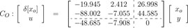$\mathsf{v}\mathsf{e}\mathsf{r}\left({\mathbb{X}}_0\right)=\left\{\left[\begin{array}{c}\hfill 1\hfill \\ \hfill 1\hfill \end{array}\right],\left[\begin{array}{c}\hfill 1\hfill \\ \hfill -1\hfill \end{array}\right]\right\},$ and then the state transformation matrix T is obtained as $10^{-3}\times \left[\begin{array}{cc}\hfill 27.827\hfill & \hfill 5.578\hfill \\ \hfill 0.835\hfill & \hfill -0.505\hfill \end{array}\right]$ with γ = 2.154. The numbers of LMI rows and decision variables in LMIs are 20 and 47, respectively. The correspondingly calculated C_O with Z being 0 is shown as(38)

We show the simulation results using controllers C_G, C_L, and C_O in Figure 1 and show the finite-time state estimation performance, i.e., ${\int }_0^3{(\mathrm{\Delta }{x}_1)}^2+{(\mathrm{\Delta }{x}_2)}^2\mathrm{d}\mathrm{t}$, in Table 1. Although the estimation of the first state of the plant system by C_L is faithful, the second state of C_L initially moves in the opposite direction to the second state of the plant system; in this sense, the estimation of the second state by C_L is poor.

FIGURE 1

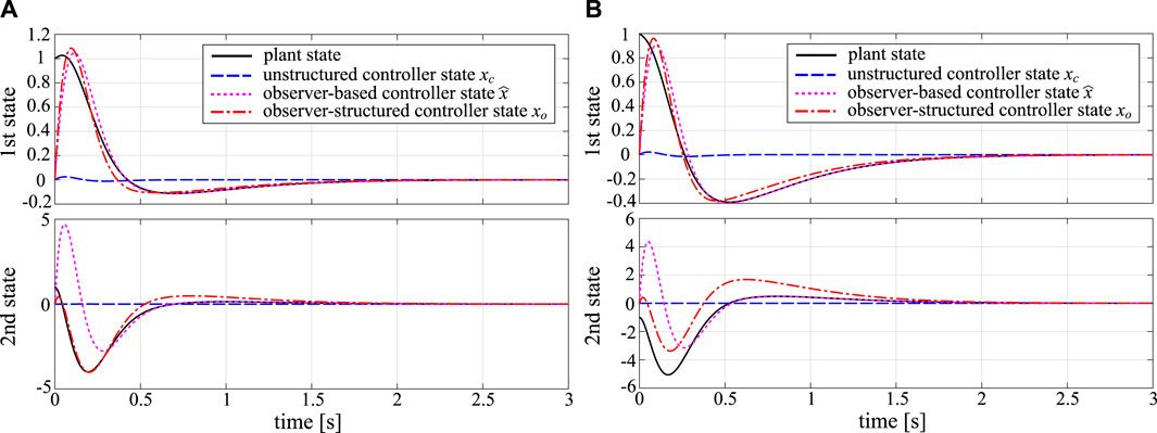
FIGURE 1. Closed-loop response to a non-zero initial plant state using C_G, C_L, and C_O: (A) $x(0)={\left[11\right]}^T$; (B) $x(0)={\left[1-1\right]}^T$.

TABLE 1

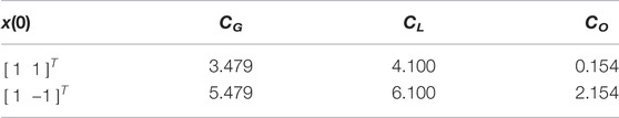
TABLE 1. State estimation performance in Figure 1.

In contrast, the observer-structured controller C_O has a much better state estimation performance as indicated in Table 1. This clearly illustrates the effectiveness of our method compared to the method in the study of Alazard (2012).

We next address Problem 2 with the following ϒ^des and W using the above T:

${\mathrm{\Upsilon }}^{des}=\left[\begin{array}{ccc}\hfill \ast \hfill & \hfill 0\hfill & \hfill 0\hfill \\ \hfill \ast \hfill & \hfill \ast \hfill & \hfill 0\hfill \\ \hfill \ast \hfill & \hfill \ast \hfill & \hfill \ast \hfill \end{array}\right],W=\left[\begin{array}{ccc}\hfill \ast \hfill & \hfill 1\hfill & \hfill 1\hfill \\ \hfill \ast \hfill & \hfill \ast \hfill & \hfill 1\hfill \\ \hfill \ast \hfill & \hfill \ast \hfill & \hfill \ast \hfill \end{array}\right],(39)$

where ∗ denotes the element of no interest. Solving Eq. 35 gives the following Z and the following corresponding state-space matrices of C_O:(40)

The transfer functions of C_G in Eq. 36, C_L in Eq. 37, and C_O in Eq. 38 are all calculated as $\frac{-1667s-2753}{s^2+27s+353}$. The transfer function of C_O with A_o, B_o, C_o, and D_o in Eq. 40 is also calculated as $\frac{-1667s-2753}{s^2+27s+353}$; however, the state-space matrices of C_O can have an artificially assigned special structure as in Eq. 40.

4.3 Effectiveness Demonstration of Our Method for Linear Parameter-Varying Plant System

We finally consider the conversion problem for LPV plant systems. Note that the methods in the studies of Alazard and Apkarian (1999) and Alazard (2012) cannot be applied to the example shown below because the plant system is given as an LPV system.

4.3.1 CT Case

We first consider the following CT LPV system:

(41)where $\theta ={\left[\begin{array}{cc}\hfill {\theta }_1\hfill & \hfill {\theta }_2\hfill \end{array}\right]}^T$. We set that the two parameters are supposed to be frozen in the interval [0.9, 1.1]; that is, the vertex sets of Λ₁ and Λ₂ are set as follows:

$\begin{array}{c}\mathsf{v}\mathsf{e}\mathsf{r}\left({\mathrm{\Lambda }}_1\right)=\left\{\left(0.9,0\right),\left(1.1,0\right)\right\},\hfill \\ \mathsf{v}\mathsf{e}\mathsf{r}\left({\mathrm{\Lambda }}_2\right)=\left\{\left(0.9,0\right),\left(1.1,0\right)\right\}.\hfill \end{array}$

It is supposed that the following stabilizing controller is given as an unstructured controller: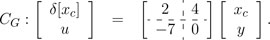(42)

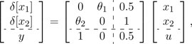
For this problem setup, we solve Eq. 29 in Lemma 1 with C_sl = [1 0] and 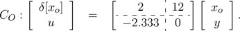$C_{s{l}_o}=1$ and obtain T = 0.333 with γ = 0.052. The numbers of LMI rows and decision variables in LMIs are 44 and 44, respectively. The state-space representation of C_O with Z = 0 is consequently given as follows:(43)

The simulation results with C_G in Eq. 42 and C_O in Eq. 43 are shown in Figure 2. It is confirmed that the state of C_O faithfully represents the plant state x₁ in both cases with x(0) = [1 0]^T and x(0) = [0 1]^T.

FIGURE 2

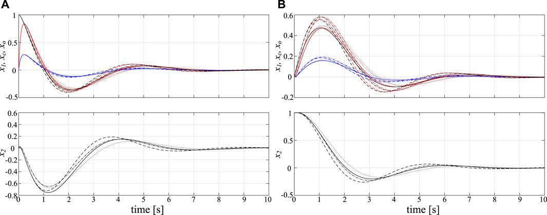
FIGURE 2. Simulation results with frozen $({\theta }_1,{\theta }_2)=\left\{(0.9,0.9),(0.9,1.1),(1.1,0.9),(1.1,1.1)\right\}$ for a CT plant (Eq. 41) with x(0) = [1 0]^T (A) and x(0) = [0 1]^T (B) (black: plant; blue: C_G in Eq. 42; red: C_O in Eq. 43).

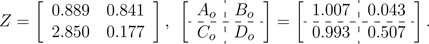
We next address Problem 2 with the following ϒ^des and W using the above T:

${\mathrm{\Upsilon }}^{des}=\left[\begin{array}{cc}\hfill 0\hfill & \hfill \ast \hfill \\ \hfill \ast \hfill & \hfill 0\hfill \end{array}\right],W=\left[\begin{array}{cc}\hfill 1\hfill & \hfill \ast \hfill \\ \hfill \ast \hfill & \hfill 1\hfill \end{array}\right],(44)$

where ∗ denotes the element of no interest. Solving Eq. 35 gives the following Z and the following corresponding state-space matrices of C_O:

.(45)

The transfer functions of C_G in Eq. 42 and C_O in Eq. 43 are both calculated as $-\frac{28}{s-2}$. The transfer function of C_O with A_o, B_o, C_o, and D_o in Eq. 45 is also calculated as $-\frac{28}{s-2}$; however, the state-space matrices of C_O can have an artificially assigned special structure as in Eq. 45.

4.3.2 DT Case

We next consider the discretized system of Eq. 41 by using Euler approximation with the sampling period ΔT = 0.1 (s):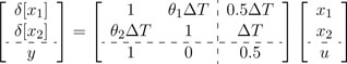 .(46)

We now set that θ₁ can vary arbitrarily fast within the interval; however, θ₂ is set as frozen in the interval; that is, the following vertex sets are considered:

$\begin{array}{c}\mathsf{v}\mathsf{e}\mathsf{r}\left({\mathrm{\Lambda }}_1\right)=\left\{\left(0.9,0.9\right),\left(0.9,1.1\right),\left(1.1,0.9\right),\left(1.1,1.1\right)\right\},\hfill \\ \mathsf{v}\mathsf{e}\mathsf{r}\left({\mathrm{\Lambda }}_2\right)=\left\{\left(0.9,0.9\right),\left(1.1,1.1\right)\right\}.\hfill \end{array}$

The controller in Eq. 42 is also discretized by using Euler approximation with the sampling period ΔT = 0.1 (s):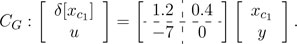(47)

For this problem setup, we solve Eq. 29 in Lemma 1 with C_sl = [1 0] and 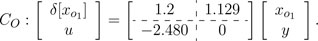$C_{s{l}_o}=1$ and obtain T = 0.353 with γ = 1.179. The numbers of LMI rows and decision variables in LMIs are 72 and 44, respectively. The state-space representation of C_O is consequently given as follows: .(48)

The simulation results with C_G in Eq. 47 and C_O in Eq. 48 are shown in Figure 3. It is indeed better to have simulations with varying θ₁ within the interval [0.9, 1.1]; however, there are uncountable combinations for the variation of θ₁. Thus, we conduct numerical simulations only with the fixed extreme points of θ₁. It is confirmed that the state of C_O faithfully represents the plant state x₁ in both cases with x(0) = [1 0]^T and x(0) = [0 1]^T.

FIGURE 3

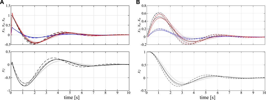
FIGURE 3. Simulation results with frozen $({\theta }_1,{\theta }_2)=\left\{(0.9,0.9),(0.9,1.1),(1.1,0.9),(1.1,1.1)\right\}$ for a DT plant (Eq. 46) with x(0) = [1 0]^T (A) and x(0) = [0 1]^T (B) (black: plant; blue: C_G in Eq. 47; red: C_O in Eq. 48).

We next address Problem 2 with the following ϒ^des and W using the above T:

${\mathrm{\Upsilon }}^{des}=\left[\begin{array}{cc}\hfill 1\hfill & \hfill 0.05\hfill \\ \hfill 1\hfill & \hfill 0.5\hfill \end{array}\right],W=\left[\begin{array}{cc}\hfill 1\hfill & \hfill 1\hfill \\ \hfill 1\hfill & \hfill 1\hfill \end{array}\right].(49)$

In this case, we set ϒ^des composed of the upper-left element of A(θ), the first element of B(θ), and the first element of C(θ) and D(θ) in the state-space matrices of Eq. 46. Our aim is to obtain matrices close to the nominal state-space matrices corresponding to the first-input-first-output system. We minimize the Frobenius norm for ϒ−ϒ^des, and obtain the following Z and the corresponding state-space matrices:

(50)

In this case, in contrast to the previously shown examples, we cannot obtain the designated figures for the state-space matrices A_o, B_o, C_o, and D_o due to lack of enough freedom in Eq. 11.

The transfer functions of C_G in Eq. 47 and C_O in Eq. 48 are both calculated as $-\frac{2.8}{z-1.2}$. The transfer function of C_O with A_o, B_o, C_o, and D_o in Eq. 50 is also calculated as $-\frac{2.8}{z-1.2}$; however, the state-space matrices of C_O can have very close figures as assigned in Eq. 49.

5 Conclusion

We address the conversion problem from unstructured LTI controllers to observer-structured LTI controllers, whose structure is similar to but not exactly the same as Luenberger observer–based controllers, for LPV systems with direct feedthrough. To this end, we first define observer-structured LTI controllers, then parameterize the state-space matrices with a priori designed unstructured LTI controller, one free matrix and a state transformation matrix, and finally propose a method which produces the optimal state transformation matrix with respect to the convergence of the discrepancy between the plant state and the observer-structured controller state for a stochastically defined non-zero initial plant state. Several toy examples are introduced to clearly illustrate the effectiveness and usefulness of observer-structured LTI controllers and the proposed method for obtaining optimal state transformation matrices with respect to the minimization between the discrepancies between the LPV plant state and the converted LTI controller state.

In this paper, we address the controller conversion problem in the case that only the stabilization problem of LPV plant systems is considered. As our next step, we are now tackling the same conversion problem in the case that some control performance criteria are also considered. Then, we will demonstrate the practicality of the conversion by using practical systems including H_∞ performance.

In this paper, it is also supposed that LTI controllers are given for LPV plant systems; however, the usefulness and effectiveness of using LPV controllers for LPV plant systems are also well recognized. Thus, the extension of our results to LPV controllers is another future research topic.

Data Availability Statement

The raw data supporting the conclusions of this article will be made available by the authors, without undue reservation.

Author Contributions

MS was in charge of theoretical development, numerical examples, and writing. NS supervised Sato’s work.

Funding

This work was conducted under the support of KAKENHI Grant Number 22K04176.

Conflict of Interest

The authors declare that the research was conducted in the absence of any commercial or financial relationships that could be construed as a potential conflict of interest.

Publisher’s Note

All claims expressed in this article are solely those of the authors and do not necessarily represent those of their affiliated organizations, or those of the publisher, the editors, and the reviewers. Any product that may be evaluated in this article, or claim that may be made by its manufacturer, is not guaranteed or endorsed by the publisher.

Acknowledgments

The authors give a sincere acknowledgement to Ms. Shikada for checking the numerical example results.

References

Alazard, D. (2012). Advances in Missile Guidance, Control, and Estmation. Boca Raton, FL: CRC Press. Chap. Control Designand Gain-Scheduling Using Observer-Based Structures. 77–128.

Google Scholar

Alazard, D., and Apkarian, P. (1999). Exact Observer-Based Structures for Arbitrary Compensators. Int. J. Robust Nonlinear Control. 9, 101–118. doi:10.1002/(sici)1099-1239(199902)9:2<101::aid-rnc400>3.0.co;2-u

CrossRef Full Text | Google Scholar

Amato, F., Mattei, M., and Pironti, A. (2005). Gain Scheduled Control for Discrete-Time Systems Depending on Bounded Rate Parameters. Int. J. Robust Nonlinear Control. 15, 473–494. doi:10.1002/rnc.1001

CrossRef Full Text | Google Scholar

Chesi, G., Garulli, A., Tesi, A., and Vicino, A. (2003). Solving Quadratic Distance Problems: An LMI-Based Approach. IEEE Trans. Automat. Contr. 48, 200–212. doi:10.1109/TAC.2002.808465

CrossRef Full Text | Google Scholar

de Oliveira, R. C. L. F., and Peres, P. L. D. (2007). Parameter-Dependent LMIs in Robust Analysis: Characterization of Homogeneous Polynomially Parameter-Dependent Solutions via LMI Relaxations. IEEE Trans. Automat. Contr. 52, 1334–1340. doi:10.1109/TAC.2007.900848

CrossRef Full Text | Google Scholar

de Oliveira, M. C., Bernussou, J., and Geromel, J. C. (1999). A New Discrete-Time Robust Stability Condition. Syst. Control. Lett. 37, 261–265. doi:10.1016/S0167-6911(99)00035-3

CrossRef Full Text | Google Scholar

Doyle, J. C., Glover, K., Khargonekar, P. P., and Francis, B. A. (1989). State-Space Solutions to Standard H/Sub 2/and H/Sub Infinity/Control Problems. IEEE Trans. Automat. Contr. 34, 831–847. doi:10.1109/9.29425

CrossRef Full Text | Google Scholar

Gahinet, P., and Apkarian, P. (1994). A Linear Matrix Inequality Approach to H∞ Control. Int. J. Robust Nonlinear Control. 4, 421–448. doi:10.1002/rnc.4590040403

CrossRef Full Text | Google Scholar

Goupil, P., Dayre, R., and Brot, P. (2014). “From Theory to Flight Tests: Airbus Flight Control System TRL5 Achievements,” in Proceedings of the 19th IFAC World Congress Cape Town, South Africa, 10562–10567. IFAC Proceedings Volumes. doi:10.3182/20140824-6-za-1003.0254747

CrossRef Full Text | Google Scholar

Iwasaki, T., and Skelton, R. E. (1994). All Controllers for the General ∞ Control Problem: LMI Existence Conditions and State Space Formulas. Automatica 30, 1307–1317. doi:10.1016/0005-1098(94)90110-4

CrossRef Full Text | Google Scholar

Masubuchi, I., Ohara, A., and Suda, N. (1998). LMI-Based Controller Synthesis: A Unified Formulation and Solution. Int. J. Robust Nonlinear Control. 8, 669–686. doi:10.1002/(sici)1099-1239(19980715)8:8<669::aid-rnc337>3.0.co;2-w

CrossRef Full Text | Google Scholar

Parrilo, P. A. (2003). Semidefinite Programming Relaxations for Semialgebraic Problems. Math. Programming 96, 293–320. doi:10.1007/s10107-003-0387-5

CrossRef Full Text | Google Scholar

Peacelle, D., and Ebihara, Y. (2018). “Affine versus Multi-Affine Models for S-Variable LMI Conditions,” in Preprints of the 9th IFAC Symposium on Robust Control Design Florianopolis, Brazil, 643–648.

Google Scholar

Peaucelle, D., Arzelier, D., Bachelier, O., and Bernussou, J. (2000). A New Robust - stability Condition for Real Convex Polytopic Uncertainty. Syst. Control. Lett. 40, 21–30. doi:10.1016/S0167-6911(99)00119-X

CrossRef Full Text | Google Scholar

Peaucelle, D., Ebihara, Y., and Hosoe, Y. (2017). Robust Observed-State Feedback Design for Discrete-Time Systems Rational in the Uncertainties. Automatica 76, 96–102. doi:10.1016/j.automatica.2016.10.003

CrossRef Full Text | Google Scholar

Peaucelle, D., and Sato, M. (2009). LMI Tests for Positive Definite Polynomials: Slack Variable Approach. IEEE Trans. Automat. Contr. 54, 886–891. doi:10.1109/TAC.2008.2010971

CrossRef Full Text | Google Scholar

Pipeleers, G., Demeulenaere, B., Swevers, J., and Vandenberghe, L. (2009). Extended LMI Characterizations for Stability and Performance of Linear Systems. Syst. Control. Lett. 58, 510–518. doi:10.1016/j.sysconle.2009.03.001

CrossRef Full Text | Google Scholar

Sampei, M., Mita, T., and Nakamichi, M. (1990). An Algebraic Approach to H∞ Output Feedback Control Problems. Syst. Control. Lett. 14, 13–24. doi:10.1016/0167-6911(90)90075-6

CrossRef Full Text | Google Scholar

Sato, M. (2020a). Observer-Based Robust Controller Design with Simultaneous Optimization of Scaling Matrices. IEEE Trans. Automat. Contr. 65, 861–866. doi:10.1109/TAC.2019.2919811

CrossRef Full Text | Google Scholar

Sato, M. (2020b). One-Shot Design of Performance Scaling Matrices and Observer-Based Gain-Scheduled Controllers Depending on Inexact Scheduling Parameters. Syst. Control. Lett. 137, 104632. doi:10.1016/j.sysconle.2020.104632

CrossRef Full Text | Google Scholar

Sato, M. (2018). Simultaneous Design of Discrete-Time Observer-Based Robust Scaled-H8 Controllers and Scaling Matrices. SICE J. Control Meas. Syst. Integration 11, 65–71. doi:10.9746/jcmsi.11.65

CrossRef Full Text | Google Scholar

Skelton, R. E., Iwasaki, T., and Grigoriadis, K. (1998). A Unified Algebraic Approach to Linear Control Design. London, UK: Taylor & Francis.

Google Scholar

Zhou, K., Doyle, J. C., and Glover, K. (1996). Robust and Optimal Control. Upper Saddle River, New Jersey: Prentice-Hall.

Google Scholar