Control of dead-time process: From the Smith predictor to general multi-input multi-output dead-time compensators

1 Introduction

In industry, as well as in other areas, many processes exhibit dead times (or delays) in their dynamic behavior. In most of the cases, the causes of dead time are energy, mass or information transportation phenomena, processing time of sensors and reaction time of actuators. Moreover, apparent dead-time can be perceived in many processes because of the dynamic effect of the accumulation of time lags in a number of simple dynamic systems connected in series (Normey-Rico and Camacho, 2007).

Even for the case of single-input and single-output (SISO) systems, the dead time complicates the feedback control design mainly because: 1) the effects of the control action and the load disturbances take some time to be felt in the controlled variable; 2) the control action that is applied based on the actual error tries to correct a situation that originated some time before. These conditions normally cause two undesirable effects on the closed-loop performance of simple loops: oscillations in the controlled and manipulated variables when the designer tries to reduce the closed-loop settling time, or very sluggish transients when the tuning avoids these oscillations (Aström and Hägglund, 1995). In the frequency domain, it is easy to understand the negative effect of dead time by simply computing the extra decrease in the system phase introduced by the delay (Normey-Rico and Camacho, 2008).

The feedback control design is even more complicated in a general multiple-input and multiple-output (MIMO) system, because, in this case, the effect of the delay is added to the coupling effects between the inputs and outputs typically observed in MIMO plants. Moreover, in the MIMO case, it is difficult to define a “process delay,” because each signal path between inputs and outputs may have a different delay (Skogestad and Postlethwaite, 2005).

One of the most used control strategies for improving the closed-loop performance of SISO and MIMO dead-time processes consists of using a predictor structure plus a primary controller. With the predictor in the loop, the primary controller can “see” an equivalent system composed by the process and the predictor, and the equivalent system exhibits no dead time or a smaller dead time than the one of the process (Normey-Rico and Camacho, 2007). These structures, which are based on the original idea of Smith proposed in 1957 (Smith, 1957), are known in the literature as dead-time compensators (DTCs), and they have been applied with success to many engineering fields, mainly in industry (Takatsu et al., 1998).

As expected, MIMO dead-time compensator structures are more difficult to analyze and tune to obtain efficient solutions. Note that MIMO-DTC strategies have to cope with nonsquare systems, different types of disturbances in each one of the controlled variables, and coupling effects. Moreover, as in the SISO case, they have to cope with unstable modes and achieve a desired robustness level. Because of this, many researchers have been working on dead-time compensators for MIMO plants during the last years, proposing particular solutions to some of the cited problems (see for example Ogunnaike and Ray (1979), Chen et al. (2011); Garrido et al. (2016)), or general structures capable to achieve a robust stable feedback control system considering a complete set of MIMO closed-loop specifications, as for instance, the works of García and Albertos (2010) and Santos et al. (2014).

This work deals with the analysis, design, and tuning of MIMO DTCs derived from the Smith Predictor when controlling stable and unstable MIMO processes with multiple delays.

The rest of the paper is organized as follows: Section 2 presents a historical perspective of the research in the topic, from the original idea of Smith in 1957 to the general MIMO-DTC solutions studied in the last years. In Section 3 the MIMO-DTC solutions for stable processes are presented. Section 4 presents MIMO-DTC solutions that can cope with integrating and unstable processes, obtaining internally stable structures. The most important aspects related to performance, robustness, and disturbance rejection are discussed in Section 5. Section 6 presents simulation and experimental case studies, followed by conclusions in Section 7.

2 Historical perspective—from the original idea of Smith to the general multi-input multi-output-dead-time compensators solutions

As already mentioned, most of the DTCs proposed in the literature were derived from the original idea of Smith, who proposed in 1957 one of the most popular dead-time compensating methods for SISO processes, called the Smith predictor (SP) (Smith, 1957). The SP is a model-based controller which separates the process model into two parts, the fast model (delay-free) and the delay model, and considers in its structure also two parts, the predictor itself and the so-called primary controller, which uses the output of the predictor to compute the control action. With this idea, the SP allows to create a virtual signal that anticipates the process output behaviour, which is used to eliminate the delay from the closed-loop characteristic equation, at least in the nominal case, in which there is no plant-model mismatch. As a consequence, the design of the closed-loop controller becomes much easier than in the original case, which contains the delay in the characteristic equation. Nowadays, the SP is the best known and most widely used algorithm for SISO dead-time compensation in academy and industry. As it was proposed to control only open-loop stable plants, several works were published after 1957 to allow its use with integrating or unstable processes. Moreover, many works studied tuning rules of the primary controller, how to improve robustness or disturbance rejection of the closed loop, and also its analysis and design in the discrete-time domain. A review of several of these proposed methods for the SISO case can be found, for example, in the book chapter (Palmor, 1996) and in the books (Normey-Rico and Camacho, 2007) and (Visioli and Zhong, 2011).

Considering MIMO processes, the first works that extended the ideas of the SP considered only the case of stable open-loop processes. In the work of Alevisakis and Seborg (1973), the authors studied MIMO stable processes with a single delay, that is, all the input-output channels of the processes are assumed to have the same dead time. For this simple case, the main properties of the SP are maintained, thus, the virtual output computed in the predictor anticipates the process output and a delay-free closed-loop characteristic equation is obtained. However, as this simple case is in general not very useful in practice, some years after this work, improved versions of this MIMO-DTC were presented, extending the results for the case of multiple delays (Ogunnaike and Ray, 1979; Jerome and Ray, 1986). In the first paper the proposed solution tries to maintain the delay-free characteristic equation of the closed-loop system, using a MIMO delay-free model with no delays, however losing the prediction property, as the obtained virtual signal is no more an anticipation of the process output. This causes a more involved tuning procedure of the controller to achieve a desired performance. The second work proposes a different fast model, in order to maintain the prediction property, however, as a consequence, obtaining a closed-loop characteristic equation with delays. Although this last property can be seen as a drawback, it is possible to show that with this choice the closed-loop performance can be improved, primarily for MIMO processes with bigger delays. Moreover, this approach gives more flexibility to the control engineer to adequate the solution to the specific characteristics of the plant, as for example, to prioritize some controlled variables against the others. Although this last solution was proposed only for square MIMO plants, the paper contains a very interesting discussion of the advantages and drawbacks of the MIMO dead-time compensation schemes. It is interesting to note that in all these approaches, the primary controller of the MIMO-DTC is in general composed by a set of PI or PID controllers. Some years later, Rao and Chidambaram (2006) and Zhang and Lin (2006) extended the ideas of the MIMO-SP to non-square stable MIMO systems with multiple time delays. In Rao and Chidambaram (2006) the authors considered the case where the process has more inputs than outputs, and, in the primary controller, a set of centralized MIMO PI controllers were tuned using a pseudo inverse of the steady-state gain matrix.

All the previously cited works focused mainly on the predictor structure. However, other works were oriented to tuning strategies for the primary controller or robustness analysis, sometimes for the general case and in other works for particular models. For example, different decoupling strategies have been analyzed along the time, optimal controllers have been proposed, first-order plus dead-time non-square systems have been analyzed, etc. In the work of Zhang and Lin (2006), a decoupled MIMO-SP is designed by factorizing the model, to separate the delay-free model into minimum phase and non-minimum phase parts, in order to analytically derive an optimal controller. In (Liu et al., 2007), the authors present an analytical decoupling scheme for square MIMO systems, based on an H₂ optimal performance specification. Stability and robustness analysis are also studied in this work; however, the procedure is valid only for stable processes. Sánchez-Peña et al. (2009) present a robust performance analysis of the MIMO-SP, but the study is limited to models in which the dead times can be factorized into input and output delays. Therefore, plants with internal coupling delays cannot be considered. A study of two inverted decoupling techniques for stable MIMO delayed processes with non-minimum-phase zeros is presented in Chen et al. (2011), and PI/PID controllers are designed for decoupled processes. Moreover, a robustness analysis is performed in the paper and low bounds of the control parameters are derived to guarantee closed-loop robust stability. In Mirkin et al. (2011), the authors convert the dead-time control problem into an equivalent delay-free problem via loop-shifting arguments, concluding that the structure of the dead-time compensator should rely upon the structure of the regulated output and/or the way in which exogenous signals affect the measurement. In Zheng et al. (2017), a discrete-time dynamic output feedback control is designed for systems with multiple dead times, considering uncertainties. A Lyapunov-Krasovskii function approach is used together with a system decomposition into two subsystems, thus facilitating the feedback controller design only based on the system output. In Bezerra-Correia et al. (2017), the authors combine the best properties of both DTC and optimal control for MIMO processes with delay. Using a state-space optimal approach, they analyze an explicit dead-time compensation structure used in model predictive control to impose desired performance and robustness properties to the closed loop. In Shaqarin et al. (2019), a robust H_∞ controller is designed using the mixed sensitivity loop shaping design.

Decoupling strategies have been extensively studied in the last years to improve the control performance of controllers for MIMO delayed systems, not limited to extensions of the MIMO-SP. In Zhang et al. (2016), an H₂ analytical decoupling control scheme with a MIMO disturbance observer is proposed. The controller can be used for both stable and unstable MIMO processes with multiple dead times. The proposed control scheme can improve the closed-loop behaviour of the system even under model mismatches and strong external disturbances. Other advantages are: 1) analytical forms of the controller and observer can be obtained, which have low orders, 2) the design procedure is simple, and 3) performance and robustness can be adjusted easily by tuning the parameters in the designed controller and observer. In Tang et al. (2018), a strategy based on a decoupling block plus an SP controller is proposed in order to reduce the negative effects of network-induced delays in the stability in MIMO networked control systems. A modified fuzzy immune feedback control algorithm is used to tune, online, the PID used in the primary controller, to improve both robustness and performance. The advantages of the algorithm proposed in Tang et al. (2018) are that it does not need to measure, estimate, or identify the network delay. In Chuong et al. (2019), a simplified decoupling strategy is proposed coupled with a MIMO-SP structure. The idea is to solve decoupling realizability by using a modified particle swarm optimization algorithm. The controller improves the system performance in terms of the servomechanism problem.

The SP can be analyzed using the more general structure of the internal model control (IMC) (Morari and Zafiriou, 1989) which enables a complete analysis of performance and robustness of the controller. Because of this, many researchers developed DTC control strategies and tuning procedures for MIMO delayed plants using the IMC approach. One of the first works was (Maciejowski, 1994), where the author analyzes the stability and robust stability of MIMO-SP considering an IMC approach. More recently, in Guo and Peng (2011), a MIMO-SP is proposed for process with right-half-plane zeros. The proposed strategy uses a decoupling compensation control method, and the IMC technique is applied to design the SP. To reduce the order of the obtained controller a sub-optimal reduction algorithm is proposed, such that the design process of the controller is simplified. In Chen et al. (2011), the authors presented an IMC approach of the MIMO-SP for a particular case, considering the elements of the MIMO model as first-order-plus-time-delay transfer functions. Later, in the work of Jin et al. (2013), the IMC is applied to an equivalent model of the plant, obtained using the concept of effective open-loop transfer function. The idea in this paper is to ease the primary PID control design, thus avoiding using decoupling strategies as in previous solutions. In Garrido et al. (2014), a new tuning method of the main controller of an IMC strategy is proposed based on the centralized inverted decoupling structure, considering square MIMO plants. The advantages of the approach are that very simple general expressions for the controller elements are obtained and filters can be used to improve the disturbance rejection without modifying the nominal set-point response.

More general strategies which allow to control unstable processes and also non-square plants have been proposed in the last years. An approach for square unstable plants was presented in García and Albertos (2010). The idea of the paper is to compute a stable predictor which copes with multiple delays and to design a controller in two parts, first using a stabilizing strategy for the delay-free model and then including extra elements to achieve some output tracking and regulation requirements. In Flesch et al. (2011), a unified MIMO-DTC for square processes with multiple delays was presented, and it can be used to control stable, integrating, and unstable dead-time MIMO processes. The proposed strategy generalizes the filtered Smith predictor (FSP) controller originally proposed in Normey-Rico and Camacho (2009) for SISO plants. An interesting feature of this approach, named MIMO-FSP, is that it compensates the minimal output dead time of each output and allows a tuning procedure considering performance and robustness specifications. An improved version of the MIMO-FSP was presented in Santos et al. (2014), that can also be used for non-square plants. In this work, the use of two different dead-time free models is analyzed in order to enable more flexibility in the controller design. Moreover, for open-loop stable processes, a tuning procedure is proposed to speed-up the closed-loop disturbance rejection response, which is an important point that was not studied in many of the previous approaches. A simplified tuning strategy of the MIMO-FSP was presented in Santos et al. (2016). In this approach, offset-free control for step references and disturbances is achieved without explicitly using integral action in the primary controller, then reducing the number of tuning parameters.

An important point to be highlighted is that these new works present results is the discrete-time domain, with control laws that are implementable without any polynomial approximation of the dead time. Moreover, in the particular case of the MIMO-FSP, any control strategy can be used in the primary controller, thus allowing to combine the predictor properties with some optimal or decoupling strategies, or even to introduce some practical aspects such as constraints in the manipulated variables or varying delays. For example, the case of time-varying dead time is studied in Normey-Rico et al. (2012) for the MIMO-FSP, using a delay-dependent Linear Matrix Inequality-based condition to compute a maximum delay interval and tolerance to model uncertainties such that the closed-loop system remains stable. In Garrido et al. (2016), the idea of the MIMO-FSP is used together with a new method to design a centralised inverted decoupling structure. The primary controller, which is applied to square stable or unstable plants, can be obtained with simple general expressions and also a simple tuning of the filters allows improving the disturbance rejection responses. In Lima et al. (2016), the idea of the FSP is combined with a model predictive control strategy to improve robustness or disturbance rejection properties of the closed loop. The controller, named filtered dynamic matrix control (FDMC), is a modification of the well-known Dynamic Matrix Control widely used in industry. In Santos et al. (2017), the MIMO-FSP is extended to reject sinusoidal disturbances in steady state. Using the same transfer matrix description of the plant, the prediction error filter is re-tuned to deal with this new type of disturbance. As in the case of the FDMC controller, the filter design can be used in model predictive controllers with inactive constraints in steady state. In Giraldo et al. (2018), a method to design a MIMO-FSP for square processes with multiple time delays is presented based on the decentralized direct decoupling structure. Under certain realizability conditions, an easy tuning of the primary controller is presented in the paper, based on the simplification of the MIMO problem to multiple single loops. More recently, in Santos et al. (2021), the authors proposed an anti-windup strategy to be used with the MIMO-FSP predictor for the case of square plants when the control input saturates. The approach is based on a causal modified implementation of the primary controller, and interestingly, the strategy does not add any tuning parameters. Stability analysis is also presented in the paper using linear matrix inequality conditions.

Applications of the predictor ideas of the SP and FSP to nonlinear systems also appear in literature. The main idea in these works is to separate the delay from the nonlinear model of the process and combine an SP or an FSP with a nonlinear controller, in such a way that the predictor compensates the delay and the nonlinear controller is only designed for the delay-free model. For example, in Gálvez-Carrillo et al., (2007), the authors present the application of a Smith-predictor-based nonlinear predictive controller to a solar power plant. Chapter 13 of Normey-Rico and Camacho (2007) is dedicated to analyze the use of the predictor structure in the nonlinear case, and in Lima et al. (2015), a robust nonlinear FSP which extends the robustness properties of the prediction filter to the nonlinear case is presented.

As can be seen from the previous analysis there is a historical and conceptual line going from the original SP used to control SISO stable plants and arriving to the MIMO-FSP which allows to control even unstable processes with multiple delays. Thus, in the following sections a review of the main ideas of these developments are presented, directly in the discrete-time domain.

3 Simple multi-input multi-output-dead-time compensators for stable plants

This section presents the fundamental properties of the DTC for MIMO stable processes. The original Smith predictor for SISO systems is briefly revisited to point out some of the MIMO dead-time compensation challenges.

3.1 A brief review of the single-input and single-output-Smith predictor

In this work, the DTC analysis and properties are directly discussed in a discrete-time paradigm as the predictors are implemented in digital processors with no loss of generality. Anyway, continuous-time counterparts can be found in related works (Normey-Rico and Camacho, 2007, 2009).

The SISO SP is illustrated in Figure 1, where P(z) = G(z)z^−d represents the process with dead time, d is the discrete-time dead time, $P_n(z)=G_n(z)z^{-d_n}$ describes a nominal model for P(z), G_n(z) is a model without delay, also known as fast model, and C(z) is a linear controller. r(k), q(k), and n(k) are, respectively, the reference, the load disturbance and the noise signals. If the modeling error is neglected (P_n(z) = P(z)), the closed-loop transfer functions from the external signals to the output are given by

$H_{yr}\left(z\right)=\frac{P_n\left(z\right)C\left(z\right)}{1+G_n\left(z\right)C\left(z\right)},(1)$

$H_{yq}\left(z\right)=P_n\left(z\right)\left[1-\frac{P_n\left(z\right)C\left(z\right)}{1+G_n\left(z\right)C\left(z\right)}\right],(2)$

$H_{yn}\left(z\right)=1-\frac{P_n\left(z\right)C\left(z\right)}{1+G_n\left(z\right)C\left(z\right)},(3)$

where $H_{yr}(z)=\mathcal{Z}\{y(k)\}/\mathcal{Z}\{r(k)\}$, $H_{yq}(z)=\mathcal{Z}\{y(k)\}/\mathcal{Z}\{q(k)\}$, and $H_{yn}(z)=\mathcal{Z}\{y(k)\}/\mathcal{Z}\{n(k)\}$.

FIGURE 1

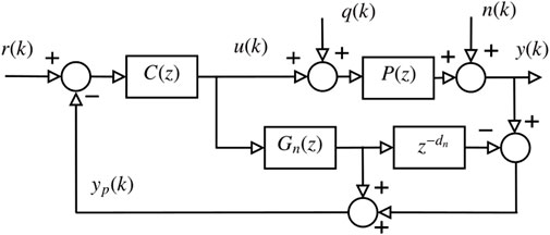
FIGURE 1. Block diagram representation of general SISO SP for stable plants.

The closed-loop requirements such as robustness margins, noise attenuation, and disturbance rejection performance are commonly defined with respect to the Sensitivity Function, namely $\mathcal{S}(z)$, and the Complementary Sensitivity Function, given by $\mathcal{C}(z)=1-\mathcal{S}(z)$. For linear closed-loop systems, the Sensitivity Function can be obtained from $\mathcal{S}(z)=H_{yn}(z)$. Hence, notice that $H_{yq}(z)=P_n(z)\mathcal{S}(z)$, and $H_{yr}(z)=\mathcal{C}(z)$.

The Smith predictor for SISO systems provides three key properties (Jerome and Ray, 1986), (Normey-Rico and Camacho, 2007, Chapter 5) in the absence of modeling error (P_n(z) = P(z)): 1) dead-time compensation, 2) output prediction, and 3) ideal dynamic compensation.

The dead-time compensation property, indicated as Property 1, comes from the fact that the delay is removed from the characteristic equation (1 + G_n(z)C(z) = 0). Hence, C(z) can be designed to define the closed-loop poles from the fast model given by G_n(z). In summary, despite the fact that the nominal process is represented by $P_n(z)=G_n(z)z^{-d_n}$, the closed-loop poles are defined by the roots of 1 + G_n(z)C(z). This property is useful as the phase margin is not reduced by $z^{-d_n}$, for instance.

Figure 1 can be used to illustrate the output prediction property of the SP, identified as Property 2 in this work. Consider the nominal case without external disturbance, then Y_p(z) = P(z)U(z) + G_n(z)U(z) − P_n(z)U(z), Y(z) = P(z)U(z) with G_n(z) = G(z), and $z^{-d}=z^{-d_n}$. Hence, $Y(z)=G_n(z)z^{-d_n}U(z)$, and Y_p(z) = G_n(z)U(z), such that y_p(k) = y(k + d). Once y(k) = y_p(k − d), the nominal set-point tracking responses can be defined for y_p(k) because y(k−d) is a direct delayed version of y_p(k). That is, the property of output prediction states that the output signal of the predictor is an anticipation of the process output. Notice that, because of this property, the nominal set-point tracking response can be designed for the delay-free predicted system from u(k) to y_p(k), which is also observed in closed loop from u(k) to y(k + d).

The Property 3 is the ideal dynamic compensation, that has been used to highlight the achievable performance bounds for input disturbance rejection. Firstly notice that the output response is given by Y(z) = H_yr(z)R(z) + H_yq(z)Q(z) + H_yn(z)N(z). If a theoretical “ideal” controller is defined with an infinity gain, then H_yr(z) → z^−d, H_yq(z) → P_n(z)[1 − z^−d], H_yn(z) → 1 − z^−d, so that Y(z) → z^−dR(z) + P_n(z)[1 − z^−d]Q(z) + [1 − z^−d]N(z). Hence, the delayed response cannot be avoided for reference changes and disturbance rejection response, which is expected due to the typical causality constraints. In summary, the achievable performance bounds depend on the delay length.

It should be highlighted that the SP cannot be used to control open-loop unstable processes because $H_{yq}(z)=P_n(z)\mathcal{S}(z)$ is not stable if P_n(z) has poles outside the unit circle. In order to achieve internal stability, modified SP versions are used, but this discussion is presented directly for the MIMO case due to the generality of the MIMO result.

3.2 Multi-input multi-output-Smith predictor—single delay case

The extension of the SP to the MIMO case with a single delay is somehow straightforward because the key ingredients are preserved (Alevisakis and Seborg, 1973). A process with single delay can be written as

$\mathbf{P}\left(z\right)=\left[\begin{array}{ccc}\hfill G_{11}{z}^{-d}\hfill & \hfill \cdots \hfill & \hfill G_{1m}{z}^{-d}\hfill \\ \hfill ⋮\hfill & \hfill \ddots \hfill & \hfill ⋮\hfill \\ \hfill G_{n1}{z}^{-d}\hfill & \hfill \cdots \hfill & \hfill G_{nm}{z}^{-d}\hfill \end{array}\right]=\left[\begin{array}{ccc}\hfill G_{11}\hfill & \hfill \cdots \hfill & \hfill G_{1m}\hfill \\ \hfill ⋮\hfill & \hfill \ddots \hfill & \hfill ⋮\hfill \\ \hfill G_{n1}\hfill & \hfill \cdots \hfill & \hfill G_{nm}\hfill \end{array}\right]z^{-d}=\mathbf{G}\left(z\right)z^{-d},(4)$

where G_ij(z)z^−d is the transfer function from the j-th input to the i-th output, being G_ij(z) a delay-free transfer function and z^−d the single time delay of the system. The matrix G(z) is known as the delay-free matrix function or fast model.

A model for the delay-free process is defined by G_n(z) and, as in the SISO case, d_n is a nominal value for d. It is simple to derive the nominal closed-loop relationship from the external signals to the output as

${\mathbf{H}}_{\text{yr}}\left(z\right)=z^{-d_n}{\mathbf{G}}_n\left(z\right)\mathbf{C}\left(z\right){\left[\mathbf{I}+{\mathbf{G}}_n\left(z\right)\mathbf{C}\left(z\right)\right]}^{-1},(5)$

${\mathbf{H}}_{\text{yq}}\left(z\right)=z^{-d_n}\left\{\mathbf{I}-z^{-d_n}{\mathbf{G}}_n\left(z\right)\mathbf{C}\left(z\right){\left[\mathbf{I}+{\mathbf{G}}_n\left(z\right)\mathbf{C}\left(z\right)\right]}^{-1}\right\}{\mathbf{G}}_n\left(z\right),(6)$

${\mathbf{H}}_{\text{yn}}\left(z\right)=\mathbf{I}-z^{-d_n}{\mathbf{G}}_n\left(z\right)\mathbf{C}\left(z\right){\left[\mathbf{I}+{\mathbf{G}}_n\left(z\right)\mathbf{C}\left(z\right)\right]}^{-1}.(7)$

Here H_yr(z) defines the matrix function between the reference vector and process variable vector, H_yq(z) defines the matrix function between the load disturbance vector and the process variable vector, and H_yn(z) defines the matrix function between the vector of measurement noise and output disturbances and the process variable vector.

Therefore, the relationships are analogous to the ones obtained in the SISO case, and the three key properties are verified for this case.

Hence, despite the fact that C(z) should be designed to deal with the MIMO closed-loop poles defined by det(I + G_n(z)C(z)) = 0, the dead-time compensation challenge is similar to the one faced in the SISO problem in the case of a single value for the input delay.

The main conclusion of this initial extension comes from the fact that the MIMO design challenge for C(z) depends on the coupling structure of G_n(z). On the other hand, the MIMO dead-time compensation challenge for the SP is similar to the SISO case if a single delay is considered. However, from a practical point of view, the single delay assumption is quite restrictive.

3.3 Multi-input multi-output-Smith predictor—multiple delay case

The first extension of SP for MIMO plants with different delays in each of the input-output pairs was proposed in Ogunnaike and Ray (1979). The idea of the method was to remove all the delays from the model of the plant to obtain a prediction structure which does not contain any delay. This approach makes the tuning of the primary controller simple with respect to the definition of the nominal closed-loop poles, since all the delays are removed from the model which is considered for the controller design. However, the prediction property of the SP (Property 2) does not hold for this case, so it is quite challenging to tune the controller to satisfy performance criteria. This idea was latter improved in Jerome and Ray (1986) to keep the prediction property and is known as generalized multidelay compensator (GMDC).

The basic idea of GMDC is to write the model of the plant as the effective time delays for each output and the remaining dynamics. GMDC is able to compensate for the effective output delays and the primary controller is responsible for guaranteeing the desired performance for the remaining dynamics. Notice that the remaining dynamics may also contain some time delays in this case, so the tuning of the primary controller may have to consider a model which still contains some delays. Consider an extension of the plant model in (Eq. 4) to consider different delays in each input-output pair given by

$\mathbf{P}\left(z\right)=\left[\begin{array}{ccc}\hfill G_{11}{z}^{-d_{11}}\hfill & \hfill \cdots \hfill & \hfill G_{1m}{z}^{-d_{1m}}\hfill \\ \hfill ⋮\hfill & \hfill \ddots \hfill & \hfill ⋮\hfill \\ \hfill G_{n1}{z}^{-d_{n1}}\hfill & \hfill \cdots \hfill & \hfill G_{nm}{z}^{-d_{nm}}\hfill \end{array}\right],(8)$

where the definitions are the same as in Eq. 4, except for d_ij, which is the discrete-time delay associated with the transfer function from the j-th input to the i-th output.

The effective time delay of each output i is d_i, which is obtained as the minimum value of the time delays associated with that particular output, i.e. $d_i={\min }_{j=1\dots m}\left(d_{ij}\right)$. Thus, defining

$\mathbf{L}\left(z\right)=\mathrm{diag}\left\{z^{-d_1},\dots ,z^{-d_n}\right\}$

as the MIMO delay of the plant model P(z), and G(z) as the model without the common delays (also known as fast model), it is possible to write the dynamics of the plant model as

$\mathbf{P}\left(z\right)=\mathbf{L}\left(z\right)\mathbf{G}\left(z\right).$

The primary controller can then be tuned to control G(z), which is given by

$\mathbf{G}\left(z\right)=\left[\begin{array}{ccc}\hfill G_{11}{z}^{-d_{11}+d_1}\hfill & \hfill \cdots \hfill & \hfill G_{1m}{z}^{-d_{1m}+d_1}\hfill \\ \hfill ⋮\hfill & \hfill \ddots \hfill & \hfill ⋮\hfill \\ \hfill G_{n1}{z}^{-d_{n1}+d_n}\hfill & \hfill \cdots \hfill & \hfill G_{nm}{z}^{-d_{nm}+d_n}\hfill \end{array}\right],$

if a control structure as the one provided in Figure 2 is used. In Figure 2, G_n(z) is the nominal fast model, L_n(z) is the nominal delay matrix, C(z) is the primary controller, and F(z) is a reference filter. In addition, r(k) is the reference vector, y(k) is the process variable vector, y_p(k) is the vector of model outputs, q(k) is a vector of load disturbances, and n(k) is a vector of measurement noise and output disturbances. For this particular structure, in the nominal case (perfect model), the transfer function matrices which define the closed-loop response are given by

${\mathbf{H}}_{\text{yr}}\left(z\right)={\mathbf{P}}_n\left(z\right)\mathbf{C}\left(z\right){\left[\mathbf{I}+{\mathbf{G}}_n\left(z\right)\mathbf{C}\left(z\right)\right]}^{-1}\mathbf{F}\left(z\right),(9)$

${\mathbf{H}}_{\text{yq}}\left(z\right)=\left\{\mathbf{I}-{\mathbf{P}}_n\left(z\right)\mathbf{C}\left(z\right){\left[\mathbf{I}+{\mathbf{G}}_n\left(z\right)\mathbf{C}\left(z\right)\right]}^{-1}\right\}{\mathbf{P}}_n\left(z\right),(10)$

${\mathbf{H}}_{\text{yn}}\left(z\right)=\mathbf{I}-{\mathbf{P}}_n\left(z\right)\mathbf{C}\left(z\right){\left[\mathbf{I}+{\mathbf{G}}_n\left(z\right)\mathbf{C}\left(z\right)\right]}^{-1}.(11)$

In order to define closed-loop design requirements and for comparison with other controllers define, respectively, the MIMO Sensitive Function and MIMO Complementary Sensitive Function, as, $\mathcal{S}(z)=\mathbf{I}-{\mathbf{P}}_n(z)\mathbf{C}(z){\left[\mathbf{I}+{\mathbf{G}}_n(z)\mathbf{C}(z)\right]}^{-1}$, and $\mathcal{C}(z)={\mathbf{P}}_n(z)\mathbf{C}(z){\left[\mathbf{I}+{\mathbf{G}}_n(z)\mathbf{C}(z)\right]}^{-1}$.

FIGURE 2

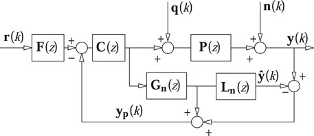
FIGURE 2. Block diagram representation of GMDC.

In this problem, it should be remarked that the fast model is given by

${\mathbf{G}}_n\left(z\right)=\left[\begin{array}{ccc}\hfill G_{n,11}{z}^{-d_{n,11}+d_{n,1}}\hfill & \hfill \cdots \hfill & \hfill G_{n,1m}{z}^{-d_{n,1m}+d_{n,1}}\hfill \\ \hfill ⋮\hfill & \hfill \ddots \hfill & \hfill ⋮\hfill \\ \hfill G_{n,n1}{z}^{-d_{n,n1}+d_{n,n}}\hfill & \hfill \cdots \hfill & \hfill G_{n,nm}{z}^{-d_{n,nm}+d_{n,n}}\hfill \end{array}\right].$

Hence, nominal prediction property holds in the absence of disturbances as Y_p(z) = G_n(z)U(z) and Y(z) = L_n(z)G_n(z)U(z). In other words, ${\mathbf{y}}_{\mathrm{p}}(k)={[y(k+d_{n,1})y(k+d_{n,2})\cdots y(k+d_{n,n})]}^{\prime }$. However, Property 1 holds partially as the characteristic equation is defined by $\det (\left[\mathbf{I}+{\mathbf{G}}_n(z)\mathbf{C}(z)\right])=0$, but G_n(z) is not a delay-free model. Clearly, the GMDC removes the effective output delay defined by L_n(z) as the controller design without DTC must consider $\det (\left[\mathbf{I}+{\mathbf{L}}_n(z){\mathbf{G}}_n(z)\mathbf{C}(z)\right])=0$. However, the advantage of the GDMC depends on the input-output dead-time for each output. The ideal compensation property (Property 3) is also preserved by using a theoretical controller with infinity gain as Y(z) → L_n(z)F(z)R(z) + P_n(z)[I − L_n(z)]Q(z) + [I − L_n(z)]N(z).

Jerome and Ray (1986) have also used the concept of rearrangement test to define whether it is possible or not to find a primary controller which at the same time provides a decoupled and best performance response. A system passes the rearrangement test if it is possible to place the minimum delay of each process variable in the main diagonal by only interchanging rows or columns. In this case, it is possible to compensate for the delays in all the loops and tune a primary controller which is able to provide a perfectly decoupled response. Based on this idea, they show that the control system performance can often be improved (or at least not degraded) by considering extra time delays in specific inputs so that the resulting system passes the rearrangement test.

As happens in the SISO case of the Smith predictor, GMDC is not able to properly deal with open-loop processes which are not strictly stable. For integrating plants, the structure is not able to reject step-like load disturbances in steady state, while for unstable systems the whole compensation structure becomes internally unstable. The extension of the ideas of GMDC for unstable plants is discussed in Section 4.

3.4 General solution for stable plants

The filtered Smith predictor for MIMO stable processes (Normey-Rico and Camacho, 2007; Flesch et al., 2011; Santos et al., 2014) is presented as a general solution for stable systems due to the design flexibility provided by the robustness filter F_r(z). The dead-time compensation properties achieved by the methods described in Ogunnaike and Ray (1979) and Jerome and Ray (1986) can be recovered from the implementation structure in Figure 3, where G_•(z) can be either a delay-free model G_f(z) or a model without the effective output delay, given by G_o(z). In this general solution, the models are given by

${\mathbf{G}}_o\left(z\right)=\left[\begin{array}{ccc}\hfill G_{n,11}{z}^{-d_{n,11}+d_{n,1}}\hfill & \hfill \cdots \hfill & \hfill G_{n,1m}{z}^{-d_{n,1m}+d_{n,1}}\hfill \\ \hfill ⋮\hfill & \hfill \ddots \hfill & \hfill ⋮\hfill \\ \hfill G_{n,n1}{z}^{-d_{n,n1}+d_{n,n}}\hfill & \hfill \cdots \hfill & \hfill G_{n,nm}{z}^{-d_{n,nm}+d_{n,n}}\hfill \end{array}\right],$

or

${\mathbf{G}}_f\left(z\right)=\left[\begin{array}{ccc}\hfill G_{n,11}\hfill & \hfill \cdots \hfill & \hfill G_{n,1m}\hfill \\ \hfill ⋮\hfill & \hfill \ddots \hfill & \hfill ⋮\hfill \\ \hfill G_{n,n1}\hfill & \hfill \cdots \hfill & \hfill G_{n,nm}\hfill \end{array}\right].$

FIGURE 3

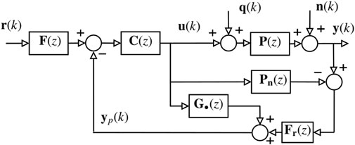
FIGURE 3. Block diagram representation of general MIMO-FSP for stable plants.

The nominal closed-loop relationships from the external signal to the output are given by

${\mathbf{H}}_{\text{yr}}\left(z\right)={\mathbf{P}}_n\left(z\right)\mathbf{C}\left(z\right){\left[\mathbf{I}+{\mathbf{G}}_{•}\left(z\right)\mathbf{C}\left(z\right)\right]}^{-1}\mathbf{F}\left(z\right),(12)$

${\mathbf{H}}_{\text{yq}}\left(z\right)=\left\{\mathbf{I}-{\mathbf{P}}_n\left(z\right)\mathbf{C}\left(z\right){\left[\mathbf{I}+{\mathbf{G}}_{•}\left(z\right)\mathbf{C}\left(z\right)\right]}^{-1}{\mathbf{F}}_r\left(z\right)\right\}{\mathbf{P}}_n\left(z\right),(13)$

${\mathbf{H}}_{\text{yn}}\left(z\right)=\mathbf{I}-{\mathbf{P}}_n\left(z\right)\mathbf{C}\left(z\right){\left[\mathbf{I}+{\mathbf{G}}_{•}\left(z\right)\mathbf{C}\left(z\right)\right]}^{-1}{\mathbf{F}}_r\left(z\right).(14)$

If G_•(z) = G_f(z) is employed in this general structure, then $\det (\left[\mathbf{I}+{\mathbf{G}}_f(z)\mathbf{C}(z)\right])=0$ is a delay-free characteristic equation. However, the prediction property does not hold in the nominal case because Y_p(z) = G_f(z)U(z), Y(z) = P_n(z)U(z), and P_n(z) ≠ L(z)G_f(z) if d_n,ij ≠ d_n,i for any j. The ideal compensation property is lost as P_n(z)C(z) ≠ L(z)G_f(z)C(z). The main consequence of this modified fast model comes from the difficulty to define C(z) with respect to performance specification as y(k) is not a direct delayed version of y_p(k). Hence, this full dead-time compensation preserves SP Property 1, but the Property 2 and Property 3 are lost.

The output feedback property and the ideal compensation properties are directly ensured if G_•(z) = G_o(z) because P_n(z) = L(z)G_o(z). Then, the GMDC properties are also verified in this case, such that $\det (\left[\mathbf{I}+{\mathbf{G}}_o(z)\mathbf{C}(z)\right])=0$ is not a delay-free characteristic equation, as previously discussed.

The proposed general structure is a filtered Smith predictor for MIMO systems where F_r(z) is a robustness filter that can be designed to deal with loop-requirement trade-offs, preserving nominal set-point tracking response. Notice that H_yr(z) does not depend on F_r(z), but $\mathcal{S}(z)=\mathbf{I}-{\mathbf{P}}_n(z)\mathbf{C}(z){\left[\mathbf{I}+{\mathbf{G}}_{•}(z)\mathbf{C}(z)\right]}^{-1}{\mathbf{F}}_r(z)$ and $\mathcal{C}(z)={\mathbf{P}}_n(z)\mathbf{C}(z){\left[\mathbf{I}+{\mathbf{G}}_{•}(z)\mathbf{C}(z)\right]}^{-1}{\mathbf{F}}_r(z)$. Indeed, for open-loop stable processes, the only internal stability requirement for F_r(z) is to be stable if the roots of $\det (\left[\mathbf{I}+{\mathbf{G}}_{•}(z)\mathbf{C}(z)\right])=0$ are inside the unit circle. This property provides a significant flexibility with respect to the definition of F_r(z). As the Complementary Sensitivity Function is directly related to the robustness filter, it becomes a powerful ingredient to deal with loop-requirement trade-offs. Conditions to achieve robust stability and deterministic disturbance rejection are discussed in Section 5.

4 Multi-input multi-output-dead-time compensators for unstable plants

The internal stability of the predictors is an important problem for unstable systems as IMC-based and SP-based strategies can be interpreted as cancellation-based control strategies. This problem is widely discussed in the DTC literature for SISO systems, but the MIMO problem is commonly neglected. This section presents the analysis of a unified MIMO-FSP for unstable processes that can be used to achieve prediction properties and to ensure internal stability.

The general MIMO-FSP can be modified to achieve internal stability by using the implementation structure presented in Figure 4, where

${\mathbf{S}}_{•}\left(z\right)={\mathbf{G}}_{•}\left(z\right)-{\mathbf{F}}_r\left(z\right){\mathbf{P}}_n\left(z\right)(15)$

is a stable filter. For analysis purposes, Figure 3 and Figure 4 are equivalent, but F_r(z) should be designed such that the minimal representation of S_•(z) has no pole outside the unit circle.

FIGURE 4

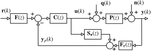
FIGURE 4. Block diagram representation of general unified MIMO-FSP for unstable systems.

The design of F_r(z) in order to achieve internal stability is not a difficult task once it can be interpreted as a combination of SISO internal stability conditions. Notice that the elements of S_•(z) are defined by S_•,ij(z) = G_•,ij(z) − F_r,ii(z)P_n,ij(z), i = 1, .., n, j = 1, .., m if F_r(z) is defined as a diagonal filter. This problem can be expressed as a determined system of linear equations where the number of decision variables is defined by the coefficient of the numerator of F_r,ii(z). In this case, the robustness filter cannot be freely defined. This stability condition can be interpreted as a loop constraint because a minimum gain is necessary to stabilize any open-loop unstable systems. The poles of F_r(z) are typically used as design parameters, but the numerators of the partial elements of the robustness filter, namely the numerators of F_r,ii(z), are used to ensure internal stability.

The stabilizing properties of S_•(z) can be explained by comparing the transfer functions of the unified solution for unstable processes with the general solution for stable systems. Assume that C(z) is a stabilizing controller such that ${\mathbf{H}}_1(z)={\mathbf{P}}_n(z){[\mathbf{I}+\mathbf{C}(z){\mathbf{G}}_{•}(z)]}^{-1}$ and ${\mathbf{H}}_2(z)={\mathbf{P}}_n(z)\mathbf{C}(z){[\mathbf{I}+{\mathbf{G}}_{•}(z)\mathbf{C}(z)]}^{-1}$ are stable transfer matrices. Hence, H_yr(z) = H₁(z)F(z) is stable if F(z) is a stable reference filter. As previously discussed, H_yn(z) = I − H₁(z)F_r(z) is also stable if F_r(z) is defined as a stable robustness filter. The transfer function from the input-disturbance to the output is similar to the one derived in the stable case, but it requires some additional manipulation as follows

$\begin{array}{ll}\hfill {\mathbf{H}}_{\text{yq}}\left(z\right)=& {\mathbf{P}}_n\left(z\right)-{\mathbf{P}}_n\left(z\right)\mathbf{C}\left(z\right){\left[\mathbf{I}+{\mathbf{G}}_{•}\left(z\right)\mathbf{C}\left(z\right)\right]}^{-1}{\mathbf{F}}_r\left(z\right){\mathbf{P}}_n\left(z\right)\hfill \\ \hfill =& {\mathbf{P}}_n\left(z\right){\left[\mathbf{I}+\mathbf{C}\left(z\right){\mathbf{G}}_{•}\left(z\right)\right]}^{-1}\left[\mathbf{I}+\mathbf{C}\left(z\right){\mathbf{G}}_{•}\left(z\right)\right]-{\mathbf{P}}_n\left(z\right)\mathbf{C}\left(z\right){\left[\mathbf{I}+{\mathbf{G}}_{•}\left(z\right)\mathbf{C}\left(z\right)\right]}^{-1}{\mathbf{F}}_r\left(z\right){\mathbf{P}}_n\left(z\right)\hfill \\ \hfill =& {\mathbf{P}}_n\left(z\right){\left[\mathbf{I}+\mathbf{C}\left(z\right){\mathbf{G}}_{•}\left(z\right)\right]}^{-1}+{\mathbf{P}}_n\left(z\right)\mathbf{C}\left(z\right)\left[{\left[\mathbf{I}+{\mathbf{G}}_{•}\left(z\right)\mathbf{C}\left(z\right)\right]}^{-1}\left[{\mathbf{G}}_{•}\left(z\right)-{\mathbf{F}}_r\left(z\right){\mathbf{P}}_n\left(z\right)\right]\right.\hfill \\ \hfill =& {\mathbf{H}}_1\left(z\right)+{\mathbf{H}}_2\left(z\right){\mathbf{S}}_{•}\left(z\right).\hfill \end{array}(16)$

This result shows that the stability of S_•(z) is required to ensure the internal stability in the MIMO problem, which is a direct extension of the SISO FSP result. Details of the complete proof can be found in Santos et al. (2014). The effects of F_r(z) on the disturbance rejection and robustness properties are discussed in Section 5.

5 Disturbance rejection and robustness

Disturbance rejection performance and robust condition define a relevant trade-off for practical control problems. The design conditions to achieve closed-loop stability in the presence plant-model mismatch and to reject persistent disturbances are even more challenging in the presence of multiple input-output delays. This section presents some of the key conditions to achieve disturbance rejection and robust stability driven to the MIMO-FSP for either stable or unstable processes.

5.1 Conditions to achieve disturbance rejection

Firstly, the rejection of constant disturbances is considered due to the relevance of this loop requirement for several applications. For presentation generality, assume that $\mathbf{n}(k)={\mathcal{Z}}^{-1}\{{\mathbf{P}}_q(z)\mathcal{Z}\{{\mathbf{q}}^{\mathbf{g}}(k)\}\}$ is a generalized disturbance signal and that its effect depends on a certain disturbance model P_q(z). For instance, if P_q(z) = P(z), then q^g(k) can be used to represent q(k), but if P_q(z) = I, then q^g(k) is equivalent to n(k). In this case, the nominal transfer matrix from q^g(k) to y(k) is given by

${\mathbf{H}}_{\text{y}{\text{q}}^{\text{g}}}\left(z\right)=\left\{\mathbf{I}-{\mathbf{P}}_n\left(z\right)\mathbf{C}\left(z\right){\left[\mathbf{I}+{\mathbf{G}}_{•}\left(z\right)\mathbf{C}\left(z\right)\right]}^{-1}{\mathbf{F}}_r\left(z\right)\right\}{\mathbf{P}}_q\left(z\right).(17)$

As the delays do not modify the static gain, then lim_z→1‖P_n(z) − G_•(z)‖ = 0 and lim_z→1‖P_n(z)C(z) − G_•(z)C(z)‖ = 0. Hence, a typical solution is to impose that F_r(1) = I and to include a multivariable integral action in C(z) such that ${\mathbf{P}}_n(1)\mathbf{C}(1){\left[\mathbf{I}+{\mathbf{G}}_{•}(1)\mathbf{C}(1)\right]}^{-1}=\mathbf{I}$ and ‖H_yq^g(1)‖ = ‖(I − I)P_q(1)‖ = 0, which ensures constant disturbance rejection for a stable P_q(z) due to the final value theorem. It should be remarked that if P_q(z) is not Bounded-Input Bounded-Output (BIBO) stable, as verified with P_q(z) = P_n(z) if P_n(z) has poles outside the unit circle, then F_r(z) has to be tuned to eliminate these poles as previously discussed based on the unified dead-time compensation structure. Therefore, S_•(z) should be stable to guarantee internal stability and ‖H_yq^g(1)‖ = 0 to ensure constant disturbance rejection. Both conditions can be handled by the design of F_r(z). The general case can be solved by defining a filter F_r(z) that guarantees the elimination of the undesired poles of P_q(z) from a minimal realization for H_yq^g(z).

An interesting interpretation of this solution based on the integral action of the primary controller C(z) comes from the fact that if the stability of S_•(z) is ensured and the filter static gain is such that ‖S_•(1)‖ = 0, then y_p(k) → y(k) in steady state and the integral action of C(z) ensures the constant disturbance rejection.

5.1.1 Modified condition to ensure constant disturbance rejection

Inspired by the ideas presented in Torrico et al. (2013) for SISO systems, a relaxed condition for constant disturbance rejection has been proposed for MIMO processes in Santos et al. (2016). Actually, the integral action may not be directly imposed by C(z), but by means of a modified steady-state condition for F_r(1). The new condition is given by: 1) S_•(1)C(1) = I for constant disturbance rejection and 2) F(1) = F_r(1) for constant set-point tracking. Moreover, if P_n(z) is stable, then S_•(1)C(1) = I can be achieved by imposing ${\mathbf{F}}_r(1)={\{{\mathbf{P}}_n(1)\mathbf{C}(1){\left[\mathbf{I}+{\mathbf{G}}_{•}(1)\mathbf{C}(1)\right]}^{-1}\}}^{-1}$. In these relaxed conditions, the disturbance rejection problem has been simplified because the integral action of C(z) is not required anymore. Notice that the previous approach with integral action is defined such that ${\{{\mathbf{P}}_n(1)\mathbf{C}(1){\left[\mathbf{I}+{\mathbf{G}}_{•}(1)\mathbf{C}(1)\right]}^{-1}\}}^{-1}=\mathbf{I}$ and F_r(1) = I, which characterizes a particular solution.

Once more, if P_q(z) is stable, then ‖H_yq^g(1)‖ = ‖(I − I)P_q(1)‖ = 0, which ensures the constant disturbance rejection due to the final value theorem. On the other hand, if P_n(z) = P_q(z) and P_n(z) has integral action, the internal stability requires that S_•(z) should be a BIBO stable matrix and the modified condition may be expressed as S_•(1)C(1) = I. The BIBO stability of S_•(z) imposes the elimination of the integrating poles of P_q(z) from the disturbance rejection response.

5.1.2 General conditions to achieve disturbance rejection

Persistent deterministic disturbances such as sinusoidal signals and ramp-like disturbances can be handled in the same final value theorem paradigm. For instance, assume that q^g(k) = A sin(ωT_sk + ϕ)I. In order to apply the final value theorem, then H_yq^g(z)Q^g(z) should be stable. As a consequence, the zeros of H_yq^g(z) should be placed in the same position of the poles of Q^g(z) over the unit circle. Hence, a new design condition is imposed to F_r(z) as follows (${\mathbf{H}}_{\text{y}{\text{q}}^{\text{g}}}(z){|}_{z=\pm e^{-j\omega T_s}}=0$ )

${\left.\left\{\mathbf{I}-{\mathbf{P}}_n\left(z\right)\mathbf{C}\left(z\right){\left[\mathbf{I}+{\mathbf{G}}_{•}\left(z\right)\mathbf{C}\left(z\right)\right]}^{-1}{\mathbf{F}}_r\left(z\right)\right\}\right|}_{z=\pm e^{-j\omega T_s}}=0.(18)$

In case of poles with multiplicity greater than one, such as q^q(k) = kA sin(ωT_sk + ϕ)I or ramp disturbances, then the condition is imposed to H_yq^g and to its derivatives, where the derivative order is one degree lower than the multiplicity of the disturbance poles.

5.1.3 Disturbance rejection performance

The unified structure of the filtered Smith predictor has been defined such that the open-loop unstable poles of P_n(z) are avoided in the transfer matrix from q(k) to y(k). This idea, that has been used to stabilize the predictor for open-loop unstable processes, can be also applied to avoid slow open-loop poles to appear in the disturbance rejection response. This solution can be implemented by defining F_r(z) such that the undesired poles of the disturbance model are eliminated from H_yq^g(z).

Once more, the transfer function from the generalized disturbance to the output is given by

${\mathbf{H}}_{\text{y}{\text{q}}^{\text{g}}}\left(z\right)=\mathcal{S}\left(z\right){\mathbf{P}}_q\left(z\right),(19)$

where $\mathcal{S}(z)=\mathbf{I}-{\mathbf{P}}_n(z)\mathbf{C}(z){\left[\mathbf{I}+{\mathbf{G}}_{•}(z)\mathbf{C}(z)\right]}^{-1}{\mathbf{F}}_r(z)$ and $\mathcal{C}(z)={\mathbf{P}}_n(z)\mathbf{C}(z){\left[\mathbf{I}+{\mathbf{G}}_{•}(z)\mathbf{C}(z)\right]}^{-1}{\mathbf{F}}_r(z)$. Hence, the Complementary Sensitivity Function and the Sensitivity Function, as a consequence, can be directly shaped by F_r(z). As a result, the disturbance rejection response can be improved, but the cost to pay comes from the typical trade-off between disturbance rejection performance and robustness.

5.2 Robustness

The robustness analysis can be performed using the standard unstructured description (Normey-Rico and Camacho, 2007). Assume that the model uncertainty can be described by

$\mathbf{P}\left(z\right)={\mathbf{P}}_n\left(z\right)+\mathbf{\Delta }\mathbf{P}\left(z\right),(20)$

where ΔP(z) is a stable unknown transfer matrix that represents plant-model mismatch (Skogestad and Postlethwaite, 2005). Moreover, the uncertainty model can be rewritten as follows¹

$\mathbf{\Delta }\mathbf{P}\left(e^{j\mathrm{\Omega }}\right)={\mathbf{W}}_2\left(e^{j\mathrm{\Omega }}\right)\mathbf{\Delta }\left(e^{j\mathrm{\Omega }}\right){\mathbf{W}}_1\left(e^{j\mathrm{\Omega }}\right),\bar{\sigma }\left(\mathbf{\Delta }\left(e^{j\mathrm{\Omega }}\right)\right)\le 1,\forall \mathrm{\Omega }\in \left[0,\pi \right].(21)$

In the Eq. 21, the functions W₁(e^jΩ) and W₂(e^jΩ) give the spatial and frequency structure of the uncertainty.

Now, define Y(z) = P_n(z)U(z) + ΔP(z)U(z), Q(z) = ΔP(z)U(z) such that: 1) Q(z) = ΔP(z)U(z) and 2) U(z) = H_uq(z)Q(z). The transfer matrix H_uq(z) is given by U(z) = −C(z)F_r(z)Q(z) − C(z)G_•(z)U(z). Then, M_•(z) = H_uq(z) is given by

${\mathbf{M}}_{•}\left(z\right)=-\left[\mathbf{I}+\mathbf{C}\left(z\right){\mathbf{G}}_{•}\left(z\right)\right]\mathbf{C}\left(z\right){\mathbf{F}}_r\left(z\right).(22)$

The robust stability condition can be derived from the Δ − M structure as depicted in Figure 5. Hence ‖Δ‖_∞‖M(z)‖_∞ < 1, where M(z) = W₁(z)M_•(z)W₂(z). Alternatively, the condition may be given by

$\bar{\sigma }\left(\mathbf{M}\left(e^{j\mathrm{\Omega }}\right)\right)<1,\forall \mathrm{\Omega }\in \left[0,\pi \right],(23)$

for block diagonal perturbations. Notice that M(z) = −W₁(z)[I + C(z)G_•(z)]C(z)F_r(z)W₂(z), such that a low-pass frequency response for F_r(z) may be directly used to reduce the loop gain at a given frequency range in order to achieve the robust stability criterion.

FIGURE 5

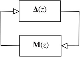
FIGURE 5. Δ − M structure for robustness analysis.

If the system is open-loop unstable, the internal stability condition implicitly imposes design constraints for F_r(z) as a minimum gain is required to stabilize the prediction. Moreover, low-pass robustness filters slow down disturbance rejection performance even for open-loop stable processes. Hence, the trade-off between disturbance rejection and robustness should be taken into account.

For presentation simplicity, the additive uncertainty description has been used in order to illustrate the robustness filter impact with respect to a robust stability criterion, but this type of simplified uncertainty description is not suitable to deal with unstable additive uncertainty terms. For the general problem, other types of uncertainty descriptions such as the multiplicative input, the multiplicative output and their inverse counterparts can be derived from the definitions presented by Skogestad and Postlethwaite (2005, Chapter 8). The proposed criterion is conservative because it spreads the uncertainty over the whole transfer matrix before defining a magnitude bound, but it is widely used in the robustness analysis of MIMO plants (Skogestad and Postlethwaite, 2005) and the robustness filter effect can be directly highlighted.

6 Case studies

This section presents three case studies. In the first one, a SISO simulated unstable process is considered, to illustrate some details of the filter implementation. In the second simulation study, a MIMO plant is used in order to illustrate some of the discussed points related to the predictor structure and disturbance rejection response. Finally, in the third one, experimental results are presented to show the applicability of the dead-time compensation strategy in practice.

6.1 single-input and single-output unstable process

In this study the FSP is tuned to control an unstable process with transfer function given by

$P\left(z\right)=\frac{0.2214z^{-10}}{z-1.221},$

and model Y(z) = P(z)[U(z) + Q(z)], where U(z) is the manipulated variable, Q(z) is the disturbance, and Y(z) is the process output. The sampling time is T_s = 0.2 s. To achieve zero steady-state error for step references, a PI controller C(z) and a reference filter F(z) are used in the primary controller of the FSP. The tuning of the primary controller is not the focus of this case study, so in order to obtain a stable closed-loop system Y(z)/R(z), being R(z) the reference signal, C(z) and F(z) can be tuned as

$C\left(z\right)=\frac{2.657z-2.496}{z-1},F\left(z\right)=\frac{0.0606z}{z-0.9394}.$

Thus, the closed-loop transfer function in the nominal case is:

$\frac{Y\left(z\right)}{R\left(z\right)}=\frac{0.0359z}{z^2-1.633z+0.6689}{z}^{-10},$

with two poles: z = 0.8166 + 0.0449j and z = 0.8166 − 0.0449j, plus the poles which characterize the delay. The step response does not present overshoot and has a setting time of about 7 s after the delay is elapsed.

In this case, the prediction filter F_r(z) has to be tuned to obtain a closed-loop disturbance rejection transfer function Y(z)/Q(z) without the open-loop pole of the model at z = 1.221, which is outside the unit circle. Moreover, the condition F_r(1) = 1 must be met to achieve the rejection of step-like disturbances in steady state. A simple first-order filter with unity steady-state gain given by

$F_r\left(z\right)=\frac{z-a}{z-b}\frac{1-b}{1-a},$

is enough to achieve both these conditions, where b is the free parameter to define the settling time of the responses and a is computed for the condition 1 − z^−dF_r(z) = 0 for z = 1.221 and the nominal delay d = 10. Note that this condition is directly derived from the SISO expression of S_• in (15), given by S(z) = G_n(z)(1 − z^−dF_r(z)), which must be stable. Thus, all the poles of G_n(z) outside the unit circle must be cancelled with the roots of the numerator of 1 − z^−dF_r(z). In this case, tuning b = 0.915 to obtain a closed-loop time response with settling time of approximately 7 s gives a = 0.9914. Thus, the resulting prediction filter is

$F_r\left(z\right)=\frac{9.843z-9.758}{z-0.915}.$

For the controller implementation, the output prediction y_p(z) is computed using:

$Y_p\left(z\right)=S\left(z\right)U\left(z\right)+F_r\left(z\right)Y\left(z\right),$

where S(z) = G_n(z)(1 − z^−dF_r(z)) = G_n(z)z^−d(z^d − F_r(z)) is stable thanks to the imposed conditions in F_r(z). Note that S(z) must be implemented eliminating the polo-zero cancellation at z = 1.221, as this value is a root of both the numerator and denominator of S(z). Thus, S(z) can be written as $S(z)=\frac{N_s(z)}{(z-0.915)z^{10}}$, being N_s(z) = [z¹⁰ + 0.3064z⁹ + 0.3743z⁸ + 0.4572z⁷ + 0.5584z⁶ + 0.6820z⁵ + 0.8330z⁴ + 1.0174z³ + 1.2427z² + 1.5178z − 7.9893] the quotient of the polynomial division when eliminating the root at z = 1.221.

The closed-loop response of the system is show in Figure 6 for a step disturbance of amplitude 1 applied at t = 0. As can be seen, the closed-loop system is stable, the disturbance is rejected in steady state, and the settling time is, as expected, about 7 s. Note that as the system has a delay of 2 s, the response is not affected by the disturbance in the first 2 s and then the system is in open loop from t = 2 s to t = 4 s, since a control action taken at t = 2 s only affects the system response after t = 4 s. Thus, the settling time of about 7 s is measured from t = 4 s to t = 11 s (for 95% of attenuation).

FIGURE 6

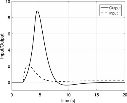
FIGURE 6. Unstable SISO system: disturbance response in closed-loop. Control action in dotted line and process output in solid line.

6.2 Multi-input multi-output integrating plant

Particularly, this case study considers the simplified MIMO-FSP. For this purpose, a challenging example of a three-stage evaporator system, already studied by several authors (Normey-Rico and Camacho 2007); (Santos et al. 2017), is chosen. A MIMO model can represent this process with two inputs, two outputs, and multiple dead times as

${\mathbf{P}}_n\left(s\right)=\left[\begin{array}{cc}\hfill \frac{3.5e^{-s}}{s}\hfill & \hfill \frac{-e^{-5s}}{2s+1}\hfill \\ \hfill \hfill & \hfill \hfill \\ \hfill \frac{2e^{-7s}}{1.5s+1}\hfill & \hfill \frac{-e^{-5s}}{3.2s+1}\hfill \end{array}\right],{\mathbf{P}}_q\left(s\right)=\left[\begin{array}{c}\hfill \frac{3.5e^{-3s}}{s}\hfill \\ \hfill \frac{-4.5e^{-2s}}{2s+1}\hfill \end{array}\right],(24)$

where the time is in minutes. The inputs are the juice and steam flows, while the outputs are the level and temperature in the storage tank. For the control design, a discrete-time model is given by

${\mathbf{P}}_n\left(z\right)=\left[\begin{array}{cc}\hfill \frac{0.7z^{-5}}{z-1}\hfill & \hfill \frac{-0.0952z^{-25}}{z-0.9048}\hfill \\ \hfill \hfill & \hfill \hfill \\ \hfill \frac{0.2497z^{-35}}{z-0.8752}\hfill & \hfill \frac{-0.0606z^{-25}}{z-0.9394}\hfill \end{array}\right],(25)$

where T_s = 0.2 min is used. Note that the output disturbance in this case is n(z) = P_q(z)q^g(z), where P_q(z) is the discrete-time model obtained from P_q(s) considering step type disturbances.

As already mentioned, one of the advantages of the simplified MIMO-FSP is that a simple primary controller C(z) can be used. In this case, for simplicity, this controller is chosen as a diagonal static gain. It is tuned to stabilize both the nominal full DTC and output DTC fast models (G_f(z) and G_o(z)). Note that these two models have, for this case study, the same elements in the diagonal, and different delays in the non-diagonal elements.

The reference filter F(z) is also a static gain that is tuned to obtain H_yr(1) = 1, then

$\mathbf{C}=\left[\begin{array}{cc}\hfill 0.2\hfill & \hfill 0\hfill \\ \hfill \hfill \\ \hfill 0\hfill & \hfill -0.2\hfill \end{array}\right],\mathbf{F}=\left[\begin{array}{cc}\hfill 1\hfill & \hfill 0\hfill \\ \hfill \hfill \\ \hfill 0\hfill & \hfill 6\hfill \end{array}\right].(26)$

The design of the robustness filter depends on the characteristic of the disturbance to be attenuated. In this study, constant and sinusoidal plus constant disturbances are considered in two different subsections. The objective is to illustrate the tuning in these two cases and to analyse different aspects of the closed-loop behavior.

6.2.1 Constant disturbance

This subsection presents comparative results of the simplified MIMO-FSP considering both full DTC and output DTC fast models and also different tuning of the robustness filters. In the first case, the filter F_r1(z) was used in the two DTCs to accelerate the disturbance rejection response; and in the second case, again for the two DTCs, a slow pole was used in F_r2(z) in order to achieve a more robust solution (Santos et al., 2014). Note that in general, the filter tuning has to satisfy a trade-off between robustness and disturbance rejection response (Santos et al., 2014), thus it is expected a better robustness in case 2. In this particular case, the used filters are

${\mathbf{F}}_{r1}\left(z\right)=\left[\begin{array}{cc}\hfill 1+12.143\frac{\left(z-1\right)}{z}\hfill & \hfill 0\hfill \\ \hfill \hfill \\ \hfill -14.286\frac{\left(z-1\right)}{z}\hfill & \hfill 6\hfill \end{array}\right],{\mathbf{F}}_{r2}\left(z\right)=\left[\begin{array}{cc}\hfill 1+0.6071\frac{\left(z-1\right)}{\left(z-0.95\right)}\hfill & \hfill 0\hfill \\ \hfill \hfill & \hfill \hfill \\ \hfill -0.7143\frac{\left(z-1\right)}{\left(z-0.95\right)}\hfill & \hfill 6\frac{0.05z}{\left(z-0.95\right)}\hfill \end{array}\right].(27)$

It is worth mentioning that for this particular case of constant disturbance, is possible to use the same robustness filter to satisfy the disturbance rejection properties for both the full and output DTC fast models. This is possible because the two models have the same transfer function in the element (1, 1) of the fast model, which is the one with the integrative mode. And, as the filter is block diagonal, the internal stability condition is achieved tuning F_r,11(z).

Figure 7 shows the simulation results. Two step changes were applied to the references r₁ and r₂ at t = 0 min and t = 20 min, respectively. Then, a constant disturbance q^g(t) = −0.02 was applied at the input of P_q(s) at t = 50 min. It can be seen that both controllers have similar performance for the first setpoint change. In the second setpoint, the process coupling affected the FSP with the full DTC fast model more severely, originating an undershoot of 37% on y₁(t). In comparison, the output DTC presented an overshoot of 18%. As expected, the robustness filters do not affect the nominal setpoint response. Regarding disturbance rejection, in the case of the more aggressive filter F_r1(z) (Figure 7A), the output y₁(t) of the output DTC presented a better response with no overshoot. However, the performance of the full DTC, for the case of F_r2(z) (see Figure 7B), was better for the same output. Finally, the disturbance rejection of the second output y₂(t) is quite similar for both controllers.

FIGURE 7

FIGURE 7. Three-stage evaporator system: constant disturbance. (A) Results for the robustness filter F_r1(z); (B) Results for the robustness filter F_r2(z);

This example shows that the process coupling and different dead times can deteriorate the setpoint response of the controller with the full DTC fast model. Thus, a reference filter may be necessary to improve the setpoint response. Furthermore, there is no general rule for disturbance attenuation because it is difficult to specify the effect of the uncompensated delays of the fast models in the responses. Thus, specific tuning rules of the MIMO-DTC is an open research topic.

6.2.2 Constant plus sinusoidal disturbances

In this subsection, the simplified FSP with output DTC fast model is compared to a model-based predictive control (MPC) implementation, which is a common choice for dealing with MIMO processes with coupling. The robustness filter is computed to obtain the desired disturbance rejection characteristics. In this case, the process is supposed to be subject to a disturbance signal which is composed of a constant part plus a sinusoidal part with a 0.7 rad/min frequency. In this case, the obtained filter F_r(z) for internal stability and sinusoidal disturbance rejection is computed using the method proposed in (Santos et al., 2017), giving

${\mathbf{F}}_r\left(z\right)=\left[\begin{array}{cc}\hfill 1+\frac{\left(z-1\right)\left(-2.7288z+2.8503\right)}{{\left(z-0.9\right)}^2}\hfill & \hfill \frac{-7.0075\left(z-1\right)}{z-0.9}\hfill \\ \hfill \hfill & \hfill \hfill \\ \hfill \frac{\left(z-1\right)\left(-6.0903z+5.9474\right)}{{\left(z-0.9\right)}^2}\hfill & \hfill 6+\frac{-14.9620\left(z-1\right)}{z-0.9}\hfill \end{array}\right].(28)$

Note that the robustness filter has the same static gain as F(z), which is necessary to obtain an integral action. In addition, for a fair comparison, all the poles of the filter F_r(z) are set to be equal to the MPC proposed in Santos et al. (2017). In order to perform the simulations, step changes were applied in the reference r₁ at t = 10 min and in r₂ at t = 50 min; a constant disturbance of amplitude −0.2 was applied at t = 120 min, and a sinusoidal disturbance defined by 0.2 sin(0.7t) was introduced at t = 180 min.

As shown in Figure 8, for this tuning, the MPC has a slightly better setpoint response because it attenuates better the process coupling using a stronger control action. In this case, the disturbance rejection response is slightly better in the simplified FSP for both constant and sinusoidal disturbances, despite the simplified FSP having filters with lower order than the adaptive MPC. It is fair to mention that the MPC uses an adaptive filter that estimates the frequency of the sinusoidal disturbance online, which causes an additional transient in the disturbance rejection responses. This last topic is out of the scope of this paper, but further details about the adaptive approach can be found in (Santos et al., 2017). Furthermore, this example shows that despite the MPC having a great ability to deal with complex MIMO time-delayed processes, the MIMO-FSP might give a similar performance.

FIGURE 8

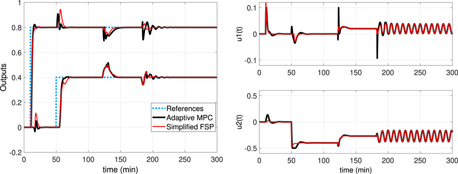
FIGURE 8. Three-stage evaporator system: constant plus sinusoidal disturbances.

6.3 Control of a neonatal intensive care unit

This section presents a practical implementation of a MIMO-DTC for controlling the temperature (T) and relative humidity (R_H) of a neonatal intensive care unit (NICU) prototype. The objective here is to illustrate, in a real case, the implementation of the MIMO-FSP, using the fast model G_o(z) in the predictor structure and considering tuning aspects for a robust behavior.

A picture of the NICU prototype and its schematic representation are shown in Figure 9. The manipulated variables of the NICU are the power of a heating resistor and a humidifier, which are controlled through a driving circuit. A fan circulates the heated and humidified air through an acrylic canopy to obtain uniform humidity and temperature in the NICU dome. The linear model of the process with a sampling time T_s = 12 s is given by Y(z) = P_n(z)U(z), where

${\mathbf{P}}_{\mathrm{n}}\left(z\right)=\left[\begin{array}{cc}\hfill \frac{0.6065z^{-4}}{z-0.9754}\hfill & \hfill \frac{-0.1678z^{-17}}{z-0.9879}\hfill \\ \hfill \hfill & \hfill \hfill \\ \hfill \frac{-0.05795z^{-15}}{z-0.9742}\hfill & \hfill \frac{0.08129z^{-14}}{z-0.9821}\hfill \end{array}\right].(29)$

FIGURE 9

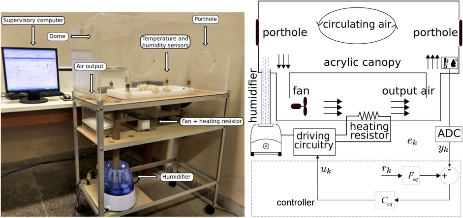
FIGURE 9. NICU prototype picture and scheme.

The output vector is given by $\mathbf{Y}={[R_{H}T]}^{\prime }$ and the input vector is $\mathbf{U}={[u_H{u}_R]}^{\prime }$, being u_H the control signal that manipulates the humidifier and u_R the one that manipulates the heating resistor.

For this case study, a diagonal PI controller C(z) is proposed, which is tuned based on the fast model, obtained by extracting the effective delay z⁻⁴ in the first output and the effective delay z⁻¹⁴ in the second output. The obtained primary controller is

$\mathbf{C}\left(z\right)=\left[\begin{array}{cc}\hfill \frac{0.0421\left(z-0.9691\right)}{z-1}\hfill & \hfill 0\hfill \\ \hfill \hfill & \hfill \hfill \\ \hfill 0\hfill & \hfill \frac{0.5934\left(z-0.985\right)}{z-1}\hfill \end{array}\right],(30)$

while the robustness filter is defined by

${\mathbf{F}}_{\mathbf{r}}\left(z\right)=\left[\begin{array}{cc}\hfill \frac{0.3883z^2-0.7503z+0.3625}{{\left(z-0.98\right)}^2}\hfill & \hfill 0\hfill \\ \hfill \hfill & \hfill \hfill \\ \hfill 0\hfill & \hfill \frac{0.01516z^2-0.0217z+0.0069}{{\left(z-0.98\right)}^2}\hfill \end{array}\right].(31)$

In this case, as the model is a simple representation of the real process, a robust tuning is used. Thus, the PI controllers do not accelerate the closed-loop responses and low-pass filters with two poles are used in the diagonal of the MIMO filter to obtain a robust closed-loop system. Moreover, this low-pass characteristic of the filters is important to attenuate the effect of the noise in the control signal.

Figure 10 shows an experiment with the proposed controller. Two setpoint changes were applied in the relative humidity and temperature setpoints to test the performance of the controller. In addition, it is worth mentioning that the unmodeled dynamics and the environmental conditions act as unknown disturbances. In Figure 10, the relative humidity (in blue) and temperature (in red) signals are at the top, while the controls signals u_H (in blue) and u_R (in red) are at the bottom. Note that the controller has a good performance, since the process outputs track the step-like references, even in the presence of unknown environmental disturbances and the coupling between the process variables. In addition, the relative humidity and temperature measurement noises are attenuated by the prediction filter and they do not affect the control signals. Furthermore, as linear controllers are used, an undesired overshoot occurs in the temperature during the first setpoint change. This effect, called windup, originated because the control signal u₂ saturates. This effect can be eliminated using an anti-windup technique, such as the one used in Santos et al. (2021), which generalizes the ideas in Flesch et al. (2017). However, that is not in the scope of this case study.

FIGURE 10

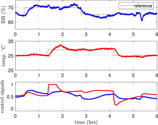
FIGURE 10. Experimental results of relative humidity and temperature control in a NICU.

7 Future research topics

As it has been analyzed in previous sections, the MIMO-FSP gives a control structure capable of dealing with stable and unstable MIMO plants with multiple delays, considering, simultaneously, several closed-loop specifications, such as disturbance rejection, robustness, and performance. All these advantages are mainly related to the predictor structure used in the controller, and to the flexibility of the predictor filter. However, from the practical control point of view, tuning aspects can be further studied. The better choice of the fast model is an important subject for research. Although, in general, the use of G_o(z) in the predictor gives good closed-loop results, there are some particular type of MIMO process, with very different delays in their elements, that can be controlled with better performance using G_f(z) as fast model. This point can be analyzed in a more general form, in order to evaluate the advantages and drawbacks of the two options and to determine which process characteristics should be considered in the decision. Another important research point is the optimal tuning of the primary controller and filters, considering a set of specifications.

This paper is based on Smith-predictor concepts for processes with multiple delays that are described by input-output transfer matrices. Input-output models are widely used in practical problems due to the identification simplicity. An interesting topic for further investigation is the extension of the DTC properties for nonlinear input-output descriptions such as Hammerstein, nonlinear autoregressive moving average with exogenous input (NARMAX), and Volterra models.

The networked control systems have introduced some interesting control challenges, such as networked induced delay, packet disorder, and data dropout. The multivariable problem with dead-time compensation in the presence of a single-input time-varying delay has already been investigated in a related work (Normey-Rico et al., 2012). However, the study of the conservativeness of the robust stability criteria for systems with time-varying delay deserves further investigation. Moreover, adaptive control strategies for system with networked induced delay and the case of multiple time-varying delays may also be interesting topics for future works.

8 Conclusion

This work presented a historical and technical overview of the design of dead-time compensators for MIMO processes with multiple dead times. It was shown how the original idea of the Smith Predictor, presented in 1957, was used in a modified form, to propose a controller capable to control MIMO stable and unstable processes satisfying a set of closed-loop specifications. It was also shown that the key point in the analysis is the correct design of the predictor structure, that has to be defined to guaranty internal stability of the closed-loop system, and to offer enough degree of freedom for tuning, looking for a trade-off between robustness and performance. This overview emphasized that the MIMO-DTC challenge depends on the internal delay structure, as different output delays may increase significantly the compensation difficulties. A unified discussion was provided such that disturbance rejection and robustness requirements can be directly handled by using any of the MIMO-FSP alternatives. The main conclusion is that the MIMO filtered Smith predictor-based controller is a generalized solution that can be used to deal with multiple loop requirements due to great flexibility provided by the robustness filter.

Author contributions

All authors contributed to conception of the work and the first draft of the manuscript. JN-R organized the historical perspective. TS and RF performed the solutions for MIMO plants. BT prepared the simulations. All authors contributed to manuscript revision, read, and approved the submitted version.

Funding

This research received funding from CNPq/Brazil—Conselho Nacional de Desenvolvimento Científico e Tecnológico—under grants 304032/2019–0, 308741/2021-8, 315546/2021-2, and 313000/2021-2.

Conflict of interest

The authors declare that the research was conducted in the absence of any commercial or financial relationships that could be construed as a potential conflict of interest.

Publisher’s note

All claims expressed in this article are solely those of the authors and do not necessarily represent those of their affiliated organizations, or those of the publisher, the editors and the reviewers. Any product that may be evaluated in this article, or claim that may be made by its manufacturer, is not guaranteed or endorsed by the publisher.

Footnotes

¹ The notation $\bar{\sigma }$(X) represents the maximum singular value of matrix X.

References

Alevisakis, G., and Seborg, D. (1973). An extension of the Smith Predictor method to multivariable linear systems containing time delays. Int. J. Control 3, 541–551. doi:10.1080/00207177308932401

CrossRef Full Text | Google Scholar

Aström, K., and Hägglund, T. (1995). PID controllers: Theory, design and tuning. Reseach Tirangle Park, NC: Instrument Society of America.

Google Scholar

Bezerra-Correia, W., Claure-Torrico, B., and Olímpio-Pereira, R. D. (2017). Optimal control of MIMO dead-time linear systems with dead-time compensation structure. Dyna 84, 62–71. doi:10.15446/dyna.v84n200.54348

CrossRef Full Text | Google Scholar

Chen, J., He, Z.-F., and Qi, X. (2011). A new control method for MIMO first order time delay non-square systems. J. Process Control 21, 538–546. doi:10.1016/j.jprocont.2011.01.007

CrossRef Full Text | Google Scholar

Chuong, V. L., Vu, T. N. L., Truong, N. T. N., and Jung, J. H. (2019). An analytical design of simplified decoupling Smith predictors for multivariable processes. Appl. Sci. 9, 2487. doi:10.3390/app9122487

CrossRef Full Text | Google Scholar

Flesch, R. C., Normey-Rico, J. E., and Flesch, C. A. (2017). A unified anti-windup strategy for SISO discrete dead-time compensators. Control Eng. Pract. 69, 50–60. doi:10.1016/j.conengprac.2017.09.002

CrossRef Full Text | Google Scholar

Flesch, R. C., Torrico, B. C., Normey-Rico, J. E., and Cavalcante, M. U. (2011). Unified approach for minimal output dead time compensation in MIMO processes. J. Process Control 21, 1080–1091. doi:10.1016/j.jprocont.2011.05.005

CrossRef Full Text | Google Scholar

Gálvez-Carrillo, M., De Keyser, R., and Ionescu, C. (2007). Application of a smith predictor based nonlinear predictive controller to a solar power plant. IFAC Proc. Vol. 40, 414–419. doi:10.3182/20070822-3-ZA-2920.00068

CrossRef Full Text | Google Scholar

García, P., and Albertos, P. (2010). Dead-time-compensator for unstable MIMO systems with multiple time delays. J. Process Control 20, 877–884. doi:10.1016/j.jprocont.2010.05.009

CrossRef Full Text | Google Scholar

Garrido, J., Vazquez, F., and Morilla, F. (2014). Inverted decoupling internal model control for square stable multivariable time delay systems. J. Process Control 24, 1710–1719. doi:10.1016/j.jprocont.2014.09.003

CrossRef Full Text | Google Scholar

Garrido, J., Vázquez, F., Morilla, F., and Normey-Rico, J. E. (2016). Smith predictor with inverted decoupling for square multivariable time delay systems. Int. J. Syst. Sci. 47, 374–388. doi:10.1080/00207721.2015.1067338

CrossRef Full Text | Google Scholar

Giraldo, S. A. C., Flesch, R. C. C., Normey-Rico, J. E., and Sejas, M. Z. P. (2018). A method for designing decoupled filtered Smith predictor for square MIMO systems with multiple time delays. IEEE Trans. Ind. Appl. 54, 6439–6449. doi:10.1109/tia.2018.2849365

CrossRef Full Text | Google Scholar

Guo, M., and Peng, Y. (2011). The control method of multivariable time-delay square system containing right half plane zeros. Procedia Eng. 15, 1004–1009. doi:10.1016/j.proeng.2011.08.186

CrossRef Full Text | Google Scholar

Jerome, N., and Ray, W. (1986). High performance multivariable control strategies for systems having time delays. AIChE J. 32, 914–931. doi:10.1002/aic.690320603

CrossRef Full Text | Google Scholar

Jin, Q., Hao, F., and Wang, Q. (2013). A multivariable IMC-PID method for non-square large time delay systems using NPSO algorithm. J. Process Control 23, 649–663. doi:10.1016/j.jprocont.2013.02.007

CrossRef Full Text | Google Scholar

Lima, D. M., Maia Santos, T. L., and Normey-Rico, J. E. (2015). “A robust predictor for nonlinear systems with dead time,” in 2015 54th IEEE Conference on Decision and Control (CDC), 7548–7553. doi:10.1109/CDC.2015.7403411

CrossRef Full Text | Google Scholar

Lima, D. M., Normey-Rico, J. E., and Santos, T. L. M. (2016). Temperature control in a solar collector field using filtered dynamic matrix control. ISA Trans. 62, 39–49. doi:10.1016/j.isatra.2015.09.016

PubMed Abstract | CrossRef Full Text | Google Scholar

Liu, T., Zhang, W., and Gao, F. (2007). Analytical decoupling control strategy using a unity feedback control structure for MIMO processes with time delays. J. Process Control 17, 173–186. doi:10.1016/j.jprocont.2006.08.010

CrossRef Full Text | Google Scholar

Maciejowski, J. (1994). Robustness of multivariable Smith predictors. J. Process Control 4, 29–32. doi:10.1016/0959-1524(94)80021-9

CrossRef Full Text | Google Scholar

Mirkin, L., Palmor, Z. J., and Shneiderman, D. (2011). Dead-time compensation for systems with multiple i/o delays: A loop-shifting approach. IEEE Trans. Autom. Contr. 56, 2542–2554. doi:10.1109/tac.2011.2108530

CrossRef Full Text | Google Scholar

Morari, M., and Zafiriou, E. (1989). Robust process control. Englewood Cliffs, NJ: Prentice-Hall.

Google Scholar

Normey-Rico, J., and Camacho, E. (2007). Control of dead-time processes. London: Springer.

Google Scholar

Normey-Rico, J., and Camacho, E. (2008). Dead-time compensators: A survey. Control Eng. Pract. 16, 407–428. doi:10.1016/j.conengprac.2007.05.006

CrossRef Full Text | Google Scholar

Normey-Rico, J. E., and Camacho, E. F. (2009). Unified approach for robust dead-time compensator design. J. Process Control 19, 38–47. doi:10.1016/j.jprocont.2008.02.003

CrossRef Full Text | Google Scholar

Normey-Rico, J. E., Garcia, P., and Gonzalez, A. (2012). Robust stability analysis of filtered Smith predictor for time-varying delay processes. J. Process Control 22, 1975–1984. doi:10.1016/j.jprocont.2012.08.012

CrossRef Full Text | Google Scholar

Ogunnaike, B., and Ray, W. (1979). Multivariable controller design for linear systems having multiple time delays. AIChE J. 25, 1043–1057. doi:10.1002/aic.690250616

CrossRef Full Text | Google Scholar

Palmor, Z. (1996). The control handbook. Time delay compensation: Smith predictor and its modifications. Mumbai: CRC Press and IEEE Press. chap. 10.8. 224–238.

Google Scholar

Rao, A., and Chidambaram, M. (2006). Smith delay compensator for multivariable non-square systems with multiple time delays. Comput. Chem. Eng. 30, 1243–1255. doi:10.1016/j.compchemeng.2006.02.017

CrossRef Full Text | Google Scholar

Sánchez-Peña, R. S., Bolea, Y., and Puig, V. (2009). MIMO Smith predictor: Global and structured robust performance analysis. J. Process Control 19, 163–177. doi:10.1016/j.jprocont.2007.12.004

CrossRef Full Text | Google Scholar

Santos, T. L., Flesch, R. C., and Normey-Rico, J. E. (2014). On the filtered Smith predictor for MIMO processes with multiple time delays. J. Process Control 24, 383–400. doi:10.1016/j.jprocont.2014.02.011

CrossRef Full Text | Google Scholar

Santos, T. L., Franklin, T. S., and Torrico, B. C. (2021). Anti-windup strategy for processes with multiple delays: A predictor-based approach. J. Frankl. Inst. 358, 1812–1838. doi:10.1016/j.jfranklin.2020.12.022

CrossRef Full Text | Google Scholar

Santos, T. L., Silva, B. P., and Uzêda, L. (2017). Multivariable filtered Smith predictor for systems with sinusoidal disturbances. Int. J. Syst. Sci. 48, 2182–2194. doi:10.1080/00207721.2017.1309591

CrossRef Full Text | Google Scholar

Santos, T. L., Torrico, B. C., and Normey-Rico, J. E. (2016). Simplified filtered Smith predictor for MIMO processes with multiple time delays. ISA Trans. 65, 339–349. doi:10.1016/j.isatra.2016.08.023

PubMed Abstract | CrossRef Full Text | Google Scholar

Shaqarin, T., Al-Rawajfeh, A., Hajaya, M., Alshabatat, N., and Noack, B. R. (2019). Model-based robust H_∞ control of a granulation process using Smith predictor with reference updating. J. Process Control 77, 38–47. doi:10.1016/j.jprocont.2019.03.003

CrossRef Full Text | Google Scholar

Skogestad, S., and Postlethwaite, I. (2005). Multivariable feedback control. Analysis and design. New York: Wiley.

Google Scholar

Smith, O. (1957). The biosynthesis of some connective tissue components. Prog. Biophys. Biophys. Chem. 53, 217–240. doi:10.1016/s0096-4174(18)30149-5

PubMed Abstract | CrossRef Full Text | Google Scholar

Takatsu, H., Itoh, T., and Araki, M. (1998). Future needs for the control theory in industries—Report and topics of the control technology survey in Japanese industry. J. Process Control 8, 369–374. doi:10.1016/s0959-1524(98)00019-5

CrossRef Full Text | Google Scholar

Tang, Y., Du, F., Cui, Y., and Zhang, Y. (2018). New Smith predictive fuzzy immune pid control algorithm for MIMO networked control systems. EURASIP J. Wirel. Commun. Netw. 1, 212–215. doi:10.1186/s13638-018-1229-8

CrossRef Full Text | Google Scholar

Torrico, B. C., Cavalcante, M. U., Braga, A. P., Normey-Rico, J. E., and Albuquerque, A. A. (2013). Simple tuning rules for dead-time compensation of stable, integrative, and unstable first-order dead-time processes. Ind. Eng. Chem. Res. 52, 11646–11654. doi:10.1021/ie401395x

CrossRef Full Text | Google Scholar

Visioli, A., and Zhong, Q.-C. (2011). Control of integral processes with dead time, 54. London: Springer.

Google Scholar

Zhang, W., and Lin, C. (2006). Multivariable Smith predictors design for nonsquare plants. IEEE Trans. Control Syst. Technol. 14, 1145–1149. doi:10.1109/tcst.2006.880219

CrossRef Full Text | Google Scholar

Zhang, W., Wang, Y., Liu, Y., and Zhang, W. (2016). Multivariable disturbance observer-based h2 analytical decoupling control design for multivariable systems. Int. J. Syst. Sci. 47, 179–193. doi:10.1080/00207721.2015.1036479

CrossRef Full Text | Google Scholar

Zheng, W., Wang, H.-b., and Zhang, Z.-m. (2017). Dynamic output feedback compensation control for discrete closed-loop nonlinear system with multiple time-delays. Math. Problems Eng. 2017, 1–11. doi:10.1155/2017/6427807

CrossRef Full Text | Google Scholar