Abstract
The period between the beginning of the Early Iron Age and the end of the Archaic Period is a time of changes and developments in the Italian Peninsula, which led to the creation of regional ethnic and political groups and to the formation of the first city-states in Western Europe. In the present study, we focus on the evolution of terrestrial route network in the Tyrrhenian region of Latium vetus as it has been hypothesized by scholars from the archeological evidence. Our main goal is to investigate the mechanisms linking decision making processes and the structure of transportation networks. We first attempted to replicate some of its features applying three models previously elaborated for the neighboring region of Southern Etruria. Since it was not possible to attain entirely satisfactory results, we modified the model that performed better in the Etruscan region by including a tunable amount of rich-get-richer bias, which improved considerably its performance. Our results suggest that coordinated decision making with a slightly unbalanced power was responsible for the peculiar characteristics of the route network topology of Latium vetus. Moreover, the mechanism implemented by this model implies that places located at favorable positions can build on their initial advantage and get more and more powerful. This fits very well with the picture elaborated by different scholars on the nature of power balance and dynamics in this region.
1 Introduction
The period between the beginning of the Early Iron Age (950/925 BC) and the end of the Archaic Age (509 BC ca) is a time of changes and developments in the Italian Peninsula, which led to the creation of regional ethnic and political groups and to the formation of the first city-states in Western Europe (the bibliography here is vast: on regional ethnic and political groups for a traditional approach, see Pallottino (1991) and for a network approach Blake (2014); on urbanization in Italy, see, e.g., Guidi (1998, 2006); Peroni (2000); Pacciarelli (2001); Bonghi Jovino (2005); Nijboer (2005); Fulminante (2014); Rendeli (2015)).
In the present study, we focus on the terrestrial route network in the Tyrrhenian region of Latium vetus (Figure 1).
Figure 1
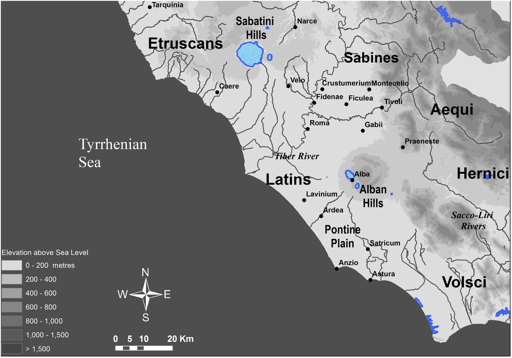
Map of the Latium vetus region and its surroundings.
Terrestrial routes can be considered as the result of the interplay of multiple factors: they are essential for permitting inter-settlement cooperative processes (information exchange, trade, defense), and at the same time, they need some level of cooperation to be established. However, since their creation and maintenance require a not negligible amount of resources, they are affected by competing interests. We can think of each connection between a pair of places as the result of a negotiation that involves the two actors but that can also be influenced, to some extent, by “third parties” as, for instance, a political authority acting on a higher level. Moreover, geographical and environmental conditions also play an important role in determining which routes are feasible and convenient. More in general, any transportation infrastructure can be regarded as the emerging outcome of social interactions and interactions between societies and environments. The importance of such systems is self-evident: they influence the development of past societies enhancing trade dynamics and affecting the prosperity of a civilization and its complexification (e.g., emergence of urbanism).
Summarizing, terrestrial routes both shape and are shaped by the societies who create them and the environment in which they exist in a very clear example of feedback loop. Therefore, understanding the development of transportation networks in a region provides insights on its social and political integration (Smith, 2005; Tuppi, 2014). In this study, we investigate what mechanisms shaped them and whether such mechanisms changed or stayed the same during the considered time framework.
We are tackling a specific aspect, but with the aim of shedding new light on the political and social dynamics between the cities that maintained those routes and connections. Specifically, we apply three non-parametric models on the region of Latium vetus, which we designed for the nearby Etruscan region (Prignano et al., 2016) in order to understand whether things worked similarly or differently in these regions.
In addition, we design a modified version of one of those models specifically for Latium vetus. By comparing the outcomes of all the four options to the empirical system, we identify some of the contributory factors that could have led Rome to prevail over other Latin cities.
2 Data Description and Methodological Approach
The set of settlements considered in the present study was used in previous works on the same region and periods (Alessandri, 2007, 2013; Fulminante, 2014). Besides settlements, the other basic element of our study is routes connecting them. Obviously, terrestrial routes for the earliest phases considered in this work have rarely been excavated, with exceptions being found mostly inside settlement areas (see, e.g., recent discoveries within the Latin center of Crustumerium (Kuusisto and Tuppi, 2009; Jarva et al., 2013), or references to road cuts in the Latin region (Tuppi, 2014)). However, they were hypothesized on the basis of later roads of Archaic and Roman time together with the position of settlements. Our starting point is the proposal of terrestrial routes provided by Lorenzo and Stefania Quilici (Colonna, 1976), which has been updated by incorporating newly discovered settlements.
According to the study of the same region in Fulminante (
2014), we divide the Iron Age into five periods that can be mapped against Latial chronology in the following way:
Early Iron Age 1 Early (EIA1E): Latial Period IIA (950/925–900 BC)
Early Iron Age 1 Late (EIA1L): Latial Period IIB (900–850/825 BC)
Early Iron Age 2 (EIA2): Latial Period III (850/825–730/720 BC)
Orientalizing Age (OA): Latial Period IVA and IVB (730/720–580 BC)
Archaic Period (AA): 580–509 BC.
Within each one of these periods, the set of settlements can be regarded as unchanging, that is, all the centers existed during most of the corresponding time interval and did not suffer any major change. We can reasonably assume that the same applies to the routes between them. In this way, we are able to reduce the analysis of the continuous evolution of settlements and routes to the study of five static time stamps.
However, the set of sites is not constant through the periods considered since they eventually appear and disappear (see the system size in Table 1). This implies that terrestrial connections are not the only evolving element in the system under consideration. On the contrary, what we observe looks like a co-evolution of settlements and routes. The foundation of new villages and cities could be the consequence of the creation of new routes or crosses while some paths may had been opened or abandoned because of the growth of some places at expenses of some others. Addressing this complex phenomenon as a whole in a diachronic perspective is not feasible at this initial stage. The goal of the present study is to understand what kind of factors may had shaped, in terms of summary statistics indicators, the terrestrial transportation network connecting a given set of settlements. Hence, we should ask ourselves to what extent it is possible to analyze the evolution of the corresponding transportation network as an independent process.
Table 1
| EIA1E | EIA1L | EIA2 | OA | AA | |
|---|---|---|---|---|---|
| Number of nodes | 93 | 93 | 107 | 93 | 78 |
| ⟨kw⟩ (km) | 29.24 | 28.35 | 30.38 | 35.22 | 37.73 |
Number of nodes and average weighted degree of the empirical networks.
In order to answer this question, we analyze the spatial distribution of settlements from period to period, concluding that they had very similar overall characteristics. As Figure 2 shows, the average distance separating a (randomly chosen) pair of locations is about 25 km, and the diameter (maximum distance between settlements) remains around 70 km across the five Ages considered. In other words, despite the set of sites being different from Age to Age at the local scale, at a macroscopic level no major changes can be observed. Therefore, we can argue that the differences we may observe across networks corresponding to different periods are not the mere consequence of different distributions (relative positions) of the entities which such routes connect.
Figure 2
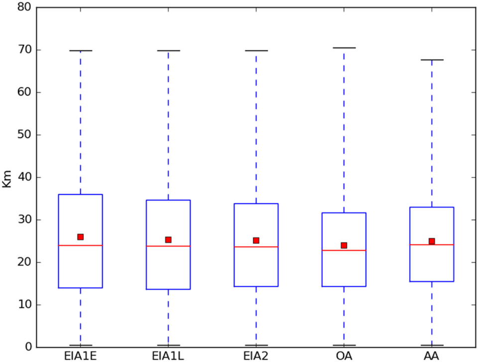
Distribution of geographical distance between pairs of settlements. Boxes stand for the second and the third quartiles, while whiskers represent the range of values. Horizontal red lines are the medians and the red squares are the means.
The question we want to address can be expressed as follows: given a set of settlements, why were the routes connecting them the way they were? Archeologists have hypothesized each route based on local evidences and considerations (local scale). However, when we look at all of them at the same time we have a transportation network with specific systemic features (at a regional scale). These systemic features are not defined by any single connection, but the whole of them together. Our goal is to identify the most important ones among them and to understand if there is some general mechanism that may explain the emergence of a system with such characteristics.
Thus, translating geographic maps into formal networks, that is, into mathematical objects that can be described and analyzed in quantitative terms, constitute an unavoidable necessity. Each settlement is represented as a geolocalized node and a bidirectional link between two sites is established whenever they were directly connected by a terrestrial route, with no other settlement in between.
After having connected sites among them, since we understand terrestrial routes as infrastructures that have to be built and maintained, it is necessary to somehow include such costs into our networks. The simplest solution is to assign to the links values (“weights”) corresponding to the linear geographic distance between the sites they connect. This is a reasonable approach providing that the region under study is relatively small and homogeneous. A more precise method to measure the aforementioned building and maintenance costs is ruled out at this point. For instance, trying to estimate the cost of each route by applying GIS based techniques would constitute a time consuming alternative that strongly relies on the precision of maps of ancient routes. Additionally, it would have with doubtful advantages for us, since our focus is on general properties of the system, not on the details of single paths. Obviously, real lengths were larger than straight lines, but by a factor that was more or less the same everywhere. Moreover, we are dealing with a compact area with a smooth landscape (i.e., without major mountain ranges, rifts, crevices, or not inhabitable areas) where the cost per kilometer of paving a new route is expected to be approximately the same everywhere.
Once the empirical system is mapped onto weighted geographical networks, we put at work the analytical toolbox provided by network science for their characterization.
Network analysis is very useful for addressing questions about “what,” i.e., what properties a system possesses. For instance, if we are interested in knowing whether a certain social relation (e.g., trust) has the transitive property (if two people trust the same person, then they are more likely to trust each other) there exist standardized techniques that can be applied. However, if we want to take a step forward investigating why we observe what we observe, then performing measurements on the empirical data is usually not enough anymore. In order to address questions about the reasons behind some observed properties, we have to devise a network model. In other words, it is necessary to hypothesize generative mechanisms that might have created the empirical network and to contrast their outcome (artificial networks) against the empirical evidence. This is exactly the main goal of the present study: to figure out if there is some general rule governing the decision-making processes that shaped the terrestrial route network.
Such decision-making process needs to be conceptualized in a simplified way, in order to become susceptible of being reformulated as a mechanism for the creation of network topologies.
Let us start considering that, in each Age, the process that produces the routes system can be described through the amount of available resources—i.e., the total link length—and a set of principles that determine the criterion for the selection of the connections. Of course, this is quite a raw simplification and it is necessary to carefully analyze its twofold implications. On the one hand, we are considering the evolution of the transportation infrastructure and the economic development of the region, which is supposed to fix the cost the system can afford in term of kilometers of routes, as separated processes. Although this is obviously not true—communication infrastructures are vital to the economic development and there is a clear feedback loop—it is also wrong to suppose that the amount of resources that can be invested in the route network is unequivocally and deterministically determined by the performance of the network itself. The amount of resources is determined by many complex factors playing a role in the development of a league of settlements that we cannot take into account quantitatively. Therefore, we regard the cost of the network at a given time as fixed externally, always taking this information from the empirical data as an input. Explaining why the total connection length varies through time is beyond the scope of this work.
We are also considering the existence of links in a given Age as something that depends only on their intrinsic importance, given the conditions (resources and principles) of that Age, without regard of whether they existed in previous times. We are thus assuming that the network has no memory. The underlying assertion is that the cost for track maintenance is comparable with the cost for creating routes anew and that no maintenance is the same as destruction. Since we are dealing with pre-roman, non-stone-paved routes, this assumption is quite realistic.
This conceptual framework sets the basis for the design of a quantitative study based on network analysis and network modeling. The first part of our study consists in the characterization of the five empirical networks, one for each Age, through appropriate topological measures. Then we make simple hypotheses about the principles that could have driven the creation of routes and translate them into mathematically well defined criteria for adding new links (generative mechanisms). Finally, we compare the synthetically generated networks with the corresponding empirical ones so that we can get insights about which criterion (or criteria), and therefore which principles, are more likely to have shaped the terrestrial communication infrastructure of the Latium vetus region in the considered time periods.
Notice that we are not aiming at reproducing each and all the connections. We just want to explain some features of the overall topology, features that we have selected for their relevance in determining the performance of such topology when understood as transportation network. This approach has the additional advantage of not being dependent on local individual details of the empirical network. As we explained above, terrestrial routes have been inferred by experts taking into account a vast heterogeneous amount of information. Hence, there is no absolute certainty on the actual existence of any of the links in the network. However, average properties of the connectivity pattern as a whole would not change noticeably if few routes were removed or replaced by equally realistic alternatives. In other words, we do not need the route map to be perfectly accurate in order for this methodology to be applied since it relies on system-scale information.
3 The Empirical Networks
Following our previous work (Prignano et al.,
2016), we characterize the empirical network through five measures:
Average weighted degree ⟨kw⟩: it measures the overall connectivity of the network, taking the weight of the edges into account. It provides, on average, the sum of the weights (lengths) of the links connected to a site.
Average edge length ⟨le⟩: it is the mean value of the weights of all the links that are present in the system.
Average clustering coefficient ⟨C⟩: among all the potential links between the neighbors of a node, the clustering coefficient indicates the proportion of them that actually exist. Averaging this ratio over the whole set of sites, we obtain a global indicator of the density of closed triangles in the network.
Global efficiency EG: the concept of efficiency implies a quantification of how well information is exchanged across the whole network. In the case of geographic networks, it is calculated as the average ratio between the geographic distance separating every pair of nodes and the length of the shortest weighted path connecting them. In doing so, we are comparing the ideal case (a geographic straight line) to the communication capability of the network (Vragović et al., 2005).
Local efficiency EL: the local efficiency of a node quantifies how well information would be exchanged between its neighbors if the node itself is removed. As in the global efficiency, weights are taken into account, so efficiencies are calculated using geographic distances and shortest weighted path lengths. The local efficiency of a network is the average local efficiency of its nodes (Vragović et al., 2005).
All these properties are calculated with network analysis software or with functions written by ourselves.1 Table 1 shows the values of the mean weighted connectivity for each Age. On average, links attached to a node sum up a total length that ranges from 28 km (for the period EIA1L) to 38 (AA). These values are complemented with the average distance length (see Figure 3). The fact that ⟨kw⟩ is 4–5 times larger implies that the mean number of links that are adjacent to a site lies between 4 and 5, since the average (unweighted) degree ⟨k⟩ is obtained by dividing ⟨kw⟩ by ⟨le⟩. Therefore, we can state that this is a highly connected region. It is also noticeable that the average edge length increases slightly through time.
Figure 3
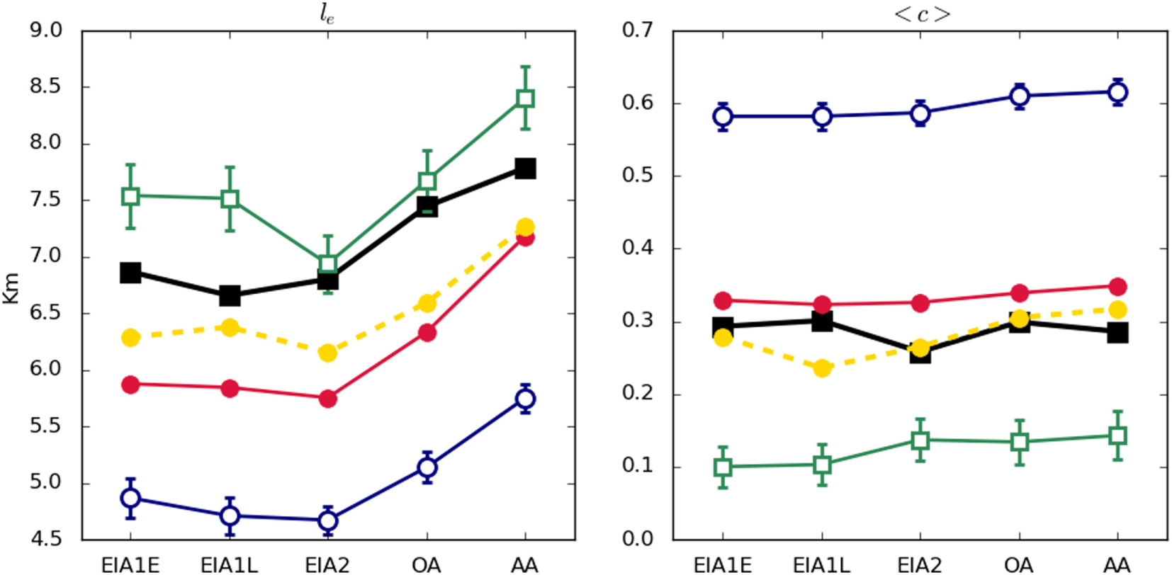
Average edge length (left) and average clustering coefficient (right). Legend: empirical network (black filled squares); averaged output of Model 1 (blue open circles); averaged output of Model 2 (green open squares); output of Model 3 (red filled circles); averaged output of Model 3PA (yellow filled circles and dashed line).
The values of the average clustering coefficient are shown in Figure 3 as well. Empirical systems present values of ⟨C⟩ around 0.3, meaning that roughly one third of the possible connections between neighbors of a site are effectively present. This represents a not negligible tendency of the system to form dense local clusters.
The efficiency of the empirical networks, both global and local, can be seen in Figure 4. They present surprisingly high values of global efficiency that remain steady along the five Ages. The local efficiency slightly increases along the periods and, while high, it is far from the one achieved for the global indicator of efficiency.
Figure 4
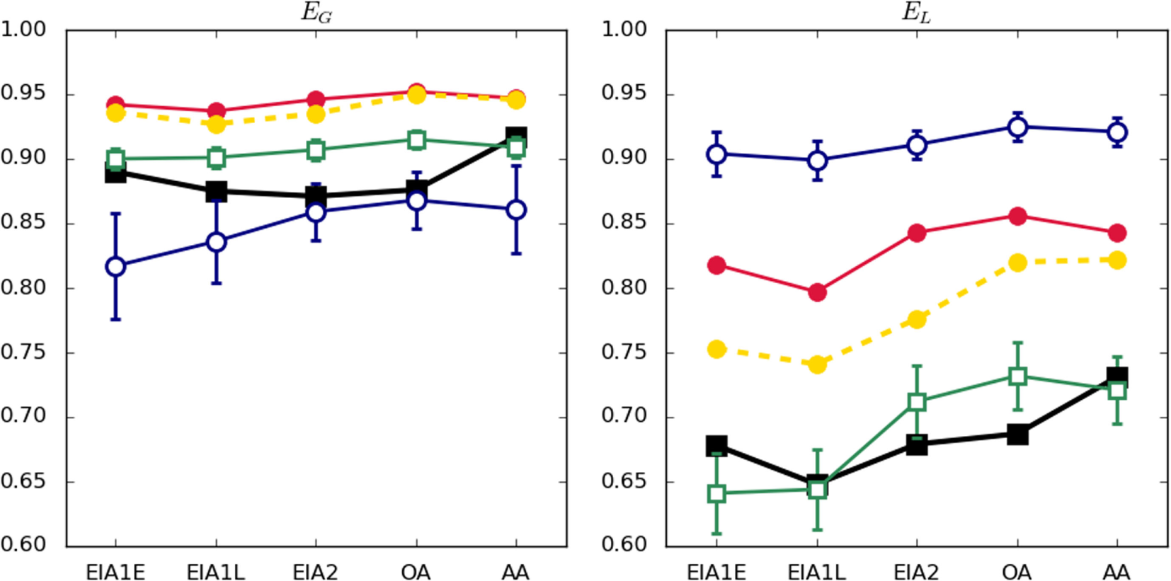
Global and local efficiencies. See legend in caption of Figure 3.
In order to understand the possible mechanisms that shaped Latium vetus terrestrial routes network, we start by applying the three models introduced in our previous study (Prignano et al., 2016).
4 Models Elaborated for the Etruscan Case Study
4.1 Model Description
The first model (Model 1) simulates a scenario of blind competition among settlements: each one of them tries to connect to as many neighbors it can, starting from the nearest one. In the second one (Model 2), we still have a scenario of competition, but this time settlements select the next place they want to connect applying a cost-benefit principle: they will connect to a settlement if it lies at a distance (cost of the new route) that is small compared to length of the shortest path to reach it that already exists. The third model (Model 3) simulates a coordinated decision-making process aimed at the minimization of weak points in the system: settlements still select the place they want to connect to according to the cost-benefit principle introduced in Model 2, but now the next settlement to gain a new link is not the one who wins some competition, but the one who needs it the most in the whole system.
For each age, we generate synthetic networks with the number of nodes and average weighted degree set equal to those of the corresponding empirical network. Then, we compare the empirical values of the remaining four structural measures with those of the model outputs. This comparative exercise allows us to hypothesize what mechanisms, among those implemented in the three models, are more likely to underlie the formation of the terrestrial networks under study. We are especially interested in checking whether Model 3, that is the one better reproducing structural properties of empirical networks in Southern Etruria, is also over-performing the other models for Latium vetus.
This procedure requires running Models 1 and 2 several times. Notice that Model 3 is deterministic, i.e., it does not include any random component. This model generates a link priority list that is univocally determined by the geographical distribution of the sites. Once the average weighted degree is set, links are created according to this list and therefore producing the same synthetic network as the only possible outcome. On the contrary Models 1 and 2 are non-deterministic (i.e., they do include certain randomness) and, consequently, we have to average over several realizations in order to obtain representative outputs. The number of realizations for each model and Age is not fixed a priori. We keep generating new ones, ten by ten, until all the structural measurements and their SDs stabilized within an error of 1%. The total amount of executions to meet this stabilization requirement ranges from 270 to 440.
4.2 Comparison with the Empirical Networks
Figures 3 and 4 show the comparison between empirical networks at each Age and their synthetic equivalents. While Model 2 seems to perform the best concerning the average edge length (Figure 3, left), Model 3 is better reproducing average clustering coefficient values (Figure 3, right).
Interestingly enough, Figure 4 shows that networks generated by Model 3 are more efficient (both globally and locally) than empirical networks in all Ages. Focusing on global efficiency, networks generated by Model 2 are the most similar to empirical ones. However, for some Ages (i.e., EIA2 and OA), outputs of Model 1 (the less globally efficient one) are more similar. Regarding local efficiency (Figure 3, right), Model 2 reproduces almost perfectly the empirical values.
Generally speaking, Model 2 seems to be the most accurate at reproducing the empirically observed behaviors, but it fails with the average clustering coefficient. On the contrary, Model 3 is the only one generating values close to the empirical ones for this magnitude. These results suggest that, in this case, the real mechanism at work was a combination of Models 2 and 3.
Actually, Model 3 is just one specific realization of Model 2. Once the focal node is selected, the criterion for determining links selection is the same for Models 2 and 3, namely minimizing the ratio r = d/L, where d is the length of the link to be created and L that of the shortest past already existing between the two nodes. What makes Models 2 and 3 different is the prioritization of nodes to be the focal one. In Model 2, all nodes have the same probability of being selected. Model 3 priorities the node minimizing r all over the system. Nevertheless, the likelihood of Model 2 to generate the same synthetic networks as Model 3 is negligible because there is a huge number of alternative orderings (N! ~ 10157). Moreover, because of the peculiarity of the ordering criterion in Model 3, these synthetic networks happen to be outliers whose values of the considered measures lie even 3–4 SDs away from the average of Model 2 (see Figures 3 and 4).
This very particular prioritization of nodes can explain why in Model 3 the values of average clustering coefficient is higher than in networks generated by Model 2. Specifically, it is much more likely for small triangles to be closed, at least when the angle between the two already existing sides is acute enough since the r value associated to the missing side is always small. As shown in Figure 2, these higher values of ⟨C⟩ are close to the empirical ones, thus desirable to our purposes.
To summarize, although both Model 2 and Model 3 capture some of the empirical features, none of them are satisfactory enough. It is noteworthy that the advantages of one correspond to the flaws of the other and viceversa, suggesting that a model placed somewhere between these two could satisfy our needs. Therefore, it becomes necessary to understand where and why Models 2 and 3 fail in order to explore our options.
5 A New Model for Latium Vetus
5.1 Model Definition
A new model explaining Latium vetus networks better should keep this convenient principle of global ordering of nodes, but should also change the specific criterion adopted. By modifying the ordering criterion, we could, in principle, interpolate between the average properties of networks of Model 2 and this very special outlier that is Model 3. However, we need some clues to modify the node ordering in a desirable way. In order to gain insight in this line, we take a closer look at both synthetic and empirical networks and, in particular, to their weighted degree and edge length distributions.
Figure 5 shows the SD of the weighted degree. In this case, Model 3 results (red circles) are much closer to the realizations of Model 2 (green open squares). Both models produce networks whose diversity among nodes in terms of weighted degree is much smaller than that observed empirically.
Figure 5
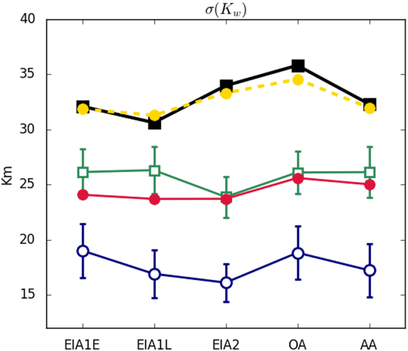
SD of the weighted degree of nodes. See legend in caption of Figure 3.
For the link length distribution we adopt a slightly different approach. We want to know where Model 2 is failing, even when considering its best realization. Hence, we need a definition of what such best realization is. We define the distance D between an empirical network and a corresponding synthetic one as: where e and s labels refer to the empirical and synthetic networks, respectively. According to this formula, distance D is obtained as the average of the absolute differences between the values of the quantities used for their characterization, the original four plus the SD of the weighted degree distribution. For quantities that are not defined in the range [0, 1], we normalize by dividing the difference by the value calculated for the empirical network.
We use this distance definition to select the synthetic networks generated by Model 2 that were the closest to the corresponding empirical ones. Then, we compare their edge length distribution with that of both empirical networks and Model 3 synthetic networks. In Figure 6, we show the boxplot of the edge lengths for ages EIA2 and OA, the two periods when the empirical average of the edge length is almost perfectly reproduced by Model 2.
Figure 6
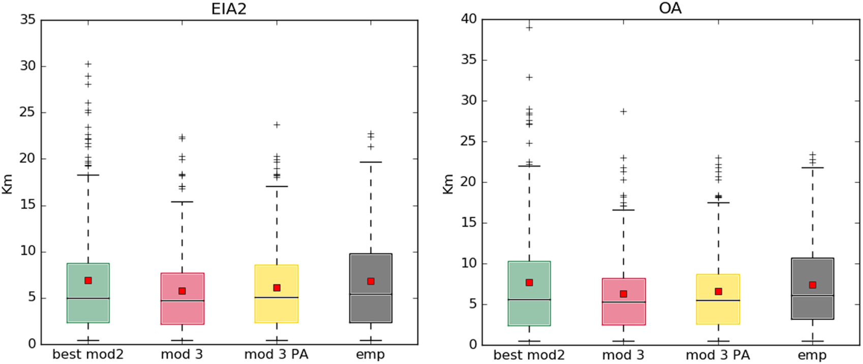
Edge length distribution of the artificial and empirical networks in the Ages EIA2 and OA.
When compared to the empirical ones, networks generated by Model 2 present a very similar average length but also many extreme outliers (i.e., with length values up to five times larger than the mean). On the contrary, Model 3 has a lower mean but similar maximum.
Taking into account these results, we conclude that empirical networks have (a) a weighted degree distribution more skewed than that of networks generated by in Models 2 and 3 and (b) an edge length distribution less skewed than the one generated by Model 2 but more than in Model 3. Consequently, in terms of identifying mechanisms capable to reproduce our empirical networks, this suggests that we are looking for a mechanism allowing the nodes to accumulate an increasing amount of connections up to a certain limit. In other words, we need nodes to compete for connections (but to a lesser extend than in Model 2), in such a way that a few privileged nodes could accumulate most of the connections.
There are obviously many ways to implement this general framework and many possible interpretations of what being a privileged node means. However, in the present study, we are interested in exploring the idea of privilege understood as the importance of a node in terms of some network measure. Such property would make some nodes more powerful and capable of imposing their priorities when new connections have to be built, thus increasing their importance even more in a positive feedback loop. Our models simulate the progressive addition of new links connecting a given set of initially disconnected nodes, but we are not reproducing the time evolution of the network. Each one of the steps of this growth corresponds to a mature state of the network but with less resources (total link length). Hence, the initial stages of the process correspond to less economically prosperous systems, not to younger ones; and the first links that the algorithms create have to be regarded as the most necessary connections, and not as the oldest ones. In this sense, if a node is very important when the growth starts, this means it is decisive when the economical situation in the region is not good. We intend such condition as an advantage that confers privileges when the system flourishes again.
In Network Science this mechanism is usually called preferential attachment and the measure for the importance of the nodes is their weighted degree, also called “node strength” (Barrat et al., 2004). The basic idea is that link creation takes into account the “power” acquired by nodes up to that point and gives a higher priority for the creation of further connections to those nodes that have a weighted degree above the average. We modified Model 3 by adding Preferential Attachment to its link generation mechanism (Model 3PA). More precisely, in Model 3PA, each node proposes the connection that is most necessary from its point of view, but the decision about which one is the next to be built is made taking into account two factors. On the one hand, we consider the objective need for that link (i.e., the value of r), on the other one, we also include in the equation the importance of the proposing node. The larger its weighted degree, the higher the priority of the link.
Mathematically, such a bias is obtained by weighting the ratio r with a (negative) power of weighted degree of the proposing node. The trade-off between the two ingredients in determining the priority of each link is tuned by the exponent a of such power. Hence, the new value of the biased ratio r′ for a connection between node i and j proposed by node i is where dij and Lij are, respectively, the geographic distance and the shortest weighted path length between them and kw(i) is the weighted degree of node i.
When a is equal to zero, there is no preferential attachment and we recover Model 3. By varying its value, starting from a = 0, one can generate networks with an increasingly biased link prioritization. The higher the value of a, the more determining the privileged condition of some nodes and less equitable principle driving the growth of the infrastructure.
5.2 Assessment of the Model Performance
For each Age, we select the value of a that generates the synthetic network whose distance to the corresponding empirical system [according to equation (1)] was minimal. Table 2 shows the obtained a values. Then, we compute all the structural measures for each one of these configurations of the new model (Model 3PA).
Table 2
| EIA1E | EIA1L | EIA2 | OA | AA | |
|---|---|---|---|---|---|
| a | 0.09 | 0.11 | 0.10 | 0.08 | 0.06 |
Values of the preferential attachment parameter a that generate the best synthetic network (the one with the shortest distance D to the empirical one) for each period.
By comparing these results with those corresponding to Models 2 and 3, we identify the following points in favor of the new model:
It is able to capture important features of the empirical system that none of the previous models could reproduce, that is, the SD of the weighted degree (see Figure 5).
Although Model 3 was already pretty good at reproducing the average clustering coefficient, the new model performs even better (see Figure 3, left).
It is almost as good as Model 2 at reproducing the average link length without the shortcoming of having some extreme outliers (see Figure 3, right, and Figure 6).
Consequently, it is the model with the shortest distance D from the empirical network for all the five Ages (Figure 7).
Overall visual inspection reveals that synthetic networks generated this way look very similar to the empirical ones, displaying the typical combination of small triangles and polygons along with few radial structures of larger connections.
It reproduces interesting structural characteristics around Rome. In particular, the city shows at the center of the most evident radial structure (see Figure 8), and it is also the node with the largest weighted degree in the EIA1L when the average is ⟨kw⟩ = (28.39 ± 31.29) km and kw (Rome) = 192.2 km.
Figure 7
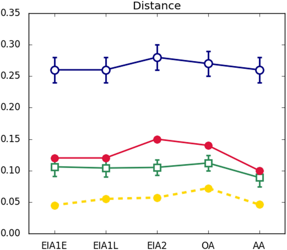
Distance D from the corresponding empirical networks. Error bars represent the SD from average for the non-deterministic models. See legend in caption of Figure 3.
Figure 8
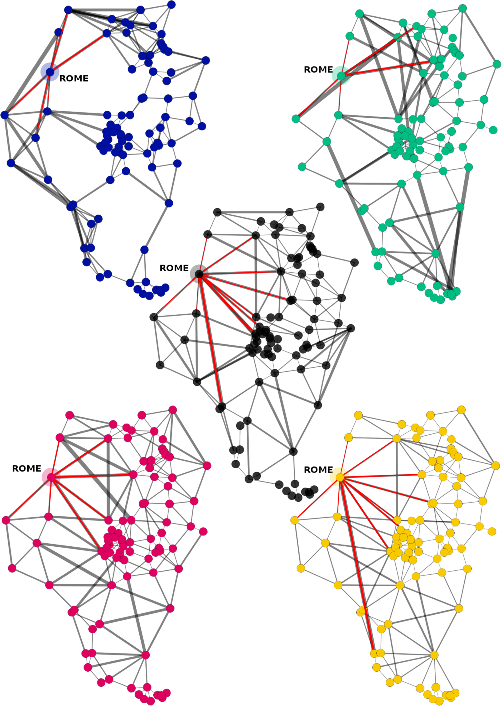
Networks of the EIA1L. Center: empirical; top left: best realization of model 1; top right: best realization of Model 2; bottom left: Model 3; bottom right: Model 3PA (optimal value of a). Connections to the node Rome are highlighted in red.
Summarizing, the best model is a modified version of Model 3 that includes weak preferential attachment (i.e., a takes small values).
Nevertheless, both the global and local efficiency of networks generated by Model 3PA are still higher than the empirical ones. We do not have an explanation for this fact yet. One possible explanation would relate such a difference with the existence of information limitations in the empirical case, which would undermine the capacity of the system to establish links according to global preferences (as it is required by Models 3 and 3PA).
6 Discussion and Conclusion
We first attempted to replicate some characterizing features of the terrestrial route network of Latium vetus, as hypothesized on the basis of available archeological and historical knowledge, using three previously elaborated models (Prignano et al., 2016). It was not possible to attain entirely satisfactory results; in particular, none of these models was able to account for the observed concentration of long range connections at few settlements. Hence, we modified one of these models—that is, the one that performed better in the Etruscan region—including a tunable amount of rich-get-richer bias, which improved considerably its performance.
Our results suggest that coordinated decision making with a slightly unbalanced power was responsible for the peculiar characteristics of the route network topology of the Latin region. This fits very well with the picture elaborated by different scholars on the nature of power balance and dynamics in the region.
Latium vetus was organized in a number of proto-urban centers and later city-states with a common material culture (Latial culture I-IV), similar burial costumes and a similar socio-political organization.2 These polities were characterized by cooperative/competitive behaviors (Renfrew, 1986; Renfrew and Cherry, 1986; Verhagen, 2015). However, the power was quite unbalanced. In particular, it seems undeniable that by the end of the EIA1E and the beginning of the EIA1L, with the shift of the funerary areas from the Forum to the Esquiline and Quirinal Hill, Rome became by far the largest settlement in the region.3
Remarkably, in the period EIA1L, Rome emerges as a hub in both the empirical network and the one generated by the biased model (Model 3PA). Notice that, since the only information our models take from the empirical data are settlement locations, a place can only be favored or disfavored by its relative position with respect to other places. Therefore, such outcome seems to confirm the hypothesis that the city occupied an advantageous position within the region. Certainly, Rome had other features that made it unique, for example, the capacity of the city of including strangers within its community [Ampolo (1976–1977, 2011) on Archaic Rome].4 However, it is very likely that its favorable location within the system of Latium vetus reinforced the concentration of power.
Interestingly, the dissimilarities in the dynamics of power among city-states of Latium vetus and its neighboring region of Southern Etruria are reflected in the difference between Models 3PA and 3 (i.e., the one best fitting the Etruscan case study). Indeed, Etruria during the Early Iron Age was dominated by a number of equally ranked proto-urban centers that went on to develop into the city-states of the Orientalizing and Archaic Period (Veii, Tarquinia, Caere, Vulci, Orvieto, and now also Bisenzio) characterized by a strong common identity5 but also by distinctive local “flavors.”6 None of these centers were able to prevail over the others and impose them a guiding role.7 Therefore, it has been suggested that at this time Etruria was characterized by a more balanced dynamics of power (Fulminante and Stoddart, 2012). This is consistent with the very good performance of a model (Model 3) that assumes an evenly distributed negotiating power among all the settlements (Prignano et al., 2016).
To conclude, this paper has presented a new model that captured some important features of the transportation network system of Latium vetus between the beginning of the Early Iron age and the Archaic Period. The mechanism implemented by this model implies that places located at favorable positions can build on their initial advantage and get more and more powerful.
There is still need for a better understanding of what a privileged position is in terms of spatial distribution of node-sites. Some additional effort should be devoted to find out what are the peculiar characteristics of the relative position of the most important sites that make them privileged. We have already discarded the most trivial options, like being located at the center of the region, since none of the sites in the central area of Latium vetus appears to be especially relevant, or having many close neighbors. However, we do not know what is special about Rome yet. Additionally, by perturbing the geographical coordinates of the nodes, we could determine how robust our results are. In particular, it is important to clarify whether Rome or some other city would have emerged if the positions of the sites had been slightly different.
Obviously many aspects were at stake in the configuration of the terrestrial route network in Latium vetus. Nonetheless, this work has shown that, provided that the interpretations are made with caution, extremely simple models can shed light on the main forces at work in complex historical processes.
Statements
Author contributions
FF, LP, and SL designed the work. FF collected the data. LP and SL devised the models. LP and IM performed the analysis. FF, LP, IM, and SL interpreted the results and drafted the paper.
Funding
LP and IM are supported by the European Research Council Advanced Grant EPNet (340828). FF is supported by the Marie Curie programme, FP7-PEOPLE-2013-IEF, Past-people-nets (628818). SL is supported by the Ramón y Cajal programme through the grant RYC-2012-01043.
Conflict of interest
The authors declare that the research was conducted in the absence of any commercial or financial relationships that could be construed as a potential conflict of interest.
Footnotes
1.^ We used Python “networkx” package to calculate the chosen properties when available as functions, whereas we wrote our own code for those that are not implemented, as well as for the model simulations. Please check the package documentation https://networkx.github.io and our repository https://github.com/ignaciomorer/frontiers for further details.
2.^ For recent accounts on the history and archaeology of the region, see Smith (2007, 2014); Carafa (2014); Fulminante (2014); Mogetta (2014).
3.^ On the importance of this shift in the development of the city of Rome, see already Guidi (1982) and more recently Carandini (1997); Alessandri (2013); Fulminante (2014).
4.^ See also reflections of ancient authors themselves such as the famous discourses by Canuleio, in Livy, IV, 3–4 and by the imperator Claudius at Lione, CIL, XIII, 1668, and Tacitus, Ann. XI, 24 quoted by Ampolo (2011), 47, or by Philippus in Polybius.
5.^ See Pacciarelli (2001) and recently Marino (2015).
6.^ On the unity but also the local variabilities within the Villanovian culture, see Bietti Sestieri (2010).
7.^ This behavior had already been captured by the application of the rank-size rule already a few years ago Guidi (1985) and also more recently Fulminante and Stoddart (2012).
References
1
Alessandri L. (2007). L’occupazione Costiera Protostorica Del Lazio Centromeridionale. Oxford: British Archaeological Reports.
2
Alessandri L. (2013). Latium Vetus in the Bronze Age and Early Iron Age/IL Latium Vetus Nell’età Del Bronzo E Nella Prima Età Del Ferro. Oxford: Archaeopress.
3
Ampolo C. (1976–1977). Demarato. Osservazioni sulla mobilità sociale arcaica. Dialoghi di Archeologia9-10: 333–45.
4
Ampolo C. (2011). I gruppi etnici in Roma arcaica: posizione del problema e fonti. In Gli Etruschi e Roma, Edited by BretschneiderG.417–433. Roma: SAGE.
5
Barrat A. Barthélemy M. Pastor-Satorras R. Vespignani A. (2004). The architecture of complex weighted networks. Proceedings of the National Academy of Sciences of the United States of America101: 3747–52.10.1073/pnas.0400087101
6
Bietti Sestieri A.M. (2010). L’Italia nell’età del bronzo e del ferro. Dalle palafitte a Romolo (220-700 a.C.). Roma: Carocci.
7
Blake E. (2014). Social Networks and Regional Identity in Bronze Age Italy. New York: Cambridge University Press.
8
Bonghi Jovino M. (2005). Città e territorio: Veio, Tarquinia, Cerveteri e Vulci, appunti e riconsiderazioni. In Dinamiche di sviluppo delle città nell’Etruria Meridionale: Veio, Caere, Tarquinia, Vulci. Atti del XXIII Convegno di Studi Etruschi ed Italici, Roma, Veio, Cerveteri/Pyrgi, Tarquinia, Tuscania, Vulci, Viterbo, 1-6 ottobre 2001, Edited by PaolettiO.CamporealeG.27–58. Roma: Istituti Editoriali e Poligrafici Internazionali.
9
Carafa P. (2014). I Latini. Prospettiva archeologica. In Entre Archéologie et Histoire: Dialogues sur divers peuples de L’Italie Preromaine, Edited by AbersonM.BiellaM.C.Di FazioM.WullschlegerM.31–50. Berne: Peter Lang.
10
Carandini A. (1997). La nascita di Roma. Dèi, lari, eroi e uomini all’alba di una civiltà. Torino: Einaudi.
11
Colonna G. (1976). Civiltà del Lazio Primitivo (Exhibition Catalogue). Roma: Multigrafica Editrice.
12
Fulminante F. (2014). The Urbanization of Rome and Latium vetus from the Bronze Age to the Archaic Era. Cambridge: Cambridge University Press.
13
Fulminante F. Stoddart S. (2012). Indigenous political dynamics and identity from a comparative perspective: Etruria and Latium vetus. In Exchange Networks and Local Transformations. Interactions and Local Changes in Europe and the Mediterranean from the Bronze Age to the Iron Age, Edited by AlbertiM.E.SabatiniS.117–133. Oxford: Oxbow Books.
14
Guidi A. (1982). Sulle prime fasi dell’urbanizzazione nel lazio protostorico. Opus1: 279–89.
15
Guidi A. (1985). An application of the rank-size rule to proto-historic settlement in the middle Tyrrhenian area. In Papers in Italian Archaeology, 4, 3. Pattern in Proto-History, Edited by StoddartS.MaloneC.217–242. Oxford: British Archaeological Reports.
16
Guidi A. (1998). The emergence of the state in central and northern Italy. Acta Archaeologica69: 139–61.
17
Guidi A. (2006). The archaeology of the early state in Italy. Social Evolution and History5: 55–90.
18
Jarva E. Kuusisto A. Lipkin S. Suuronen M. Tuppi J. (2013). Excavations in the road trench area of Crustumerium and research prospects in the future. In Crustumerium. Ricerche internazionali in un centro latino. Archaeology and Identity of a Latin Settlement Near Rome, Edited by AttemaP.Di GennaroF.JarvaE.35–44. Groningen: Groningen Institute of Archaeology.
19
Kuusisto A. Tuppi J. (2009). Research on the Crustumerium road Trench. Fasti Online Documents and Research.
20
Marino T. (2015). Aspetti e fasi del processo formativo delle città in Etruria meridionale costiera. In Le città visibili. Archeologia dei processi di formazione urbana. Vol. I: Penisola Italiana e Sardegna, Edited by RendeliM.97–141. Roma: Officina Etruscologia.
21
Mogetta M. (2014). Latium Vetus, Latium Adjectum. In Encyclopedia of Global Archaeology, Edited by SmithC.4450–4459. New York: Springer.
22
Nijboer A.J. (2005). Characteristics of emerging towns in Central Italy, 900/800 to 400 BC. In Centralization, Early Urbanization and Colonization in First Millennium BC Italy and Greece. Part 1: Italy, Edited by AttemaP.137–156. Leuven-Paris-Dudley, MA: Peeters.
23
Pacciarelli M. (2001). Dal villaggio alla città. La svolta proto-urbana del 1000 a.C. nell’Italia tirrenica. Firenze: All’Insegna del Giglio.
24
Pallottino M. (1991). A History of Earliest Italy. London: Routledge.
25
Peroni R. (2000). Formazione e sviluppi dei centri protourbani medio-tirrenici. In Roma, Romolo, Remo e la fondazione della città (Exhibition Catalogue), Edited by CarandiniA.CappelliR.26–30. Milano: Electa.
26
Prignano L. Morer I. Fulminante F. Lozano S. (2016). Modelling terrestrial route networks to understand inter-polity interactions. A case-study from Southern Etruria. Available at: https://arxiv.org/abs/1612.09321
27
Rendeli M. (2015). Le città visibili. Archeologia dei processi di formazione urbana. Vol. I: Penisola Italiana e Sardegna. Roma: Officina Etruscologia.
28
Renfrew C. (1986). Interazione fra comunità paritarie e formazione dello stato. Dialoghi di Archeologia4: 27–33.
29
Renfrew C. Cherry J.F. (1986). Peer Polity Interaction and Socio-Political Change. Cambridge: Cambridge University Press.
30
Smith C.J. (2007). Latium and the Latins: the hinterland of Rome. In Ancient Italy. Regions without Boundaries, Edited by BradleyG.IsayevE.RivaC.161–178. Exeter: University of Exeter Press.
31
Smith C.J. (2014). The Latins: historical perspective. In Entre Archéologie et Histoire: Dialogues sur divers peuples de L’Italie Preromaine, Edited by AbersonM.BiellaM.C.Di FazioM.WullschlegerM.21–30. Berne: Peter Lang.
32
Smith M.L. (2005). Networks, territories, and the cartography of ancient states. Annals of the Association of American Geographers95: 832–49.10.1111/j.1467-8306.2005.00489.x
33
Tuppi J. (2014). Approaching road-cutting as instruments of early urbanization in central Tyrrhenian Italy. Papers of the British School at Rome82: 41–72.10.1017/S006824621400004X
34
Verhagen F. (2015). Peer polity interaction in Archaic Latium Vetus: temple building as a form of competition. Tijdschrift voor Mediterrane Archeologie53: 16–21.
35
Vragović I. Louis E. Diaz-Guilera A. (2005). Efficiency of informational transfer in regular and complex networks. Physical Review. E, Statistical, Nonlinear, and Soft Matter Physics71: 036122.10.1103/PhysRevE.71.036122
Summary
Keywords
network analysis, network modeling, transportation networks, weighted networks, Latium vetus, Iron Age
Citation
Fulminante F, Prignano L, Morer I and Lozano S (2017) Coordinated Decisions and Unbalanced Power. How Latin Cities Shaped Their Terrestrial Transportation Network. Front. Digit. Humanit. 4:4. doi: 10.3389/fdigh.2017.00004
Received
17 November 2016
Accepted
23 January 2017
Published
13 February 2017
Volume
4 - 2017
Edited by
Colin D. Wren, University of Colorado, Colorado Springs, USA
Reviewed by
Alex Elias Morrison, University of Auckland, New Zealand; Heather Richards-Rissetto, University of Nebraska – Lincoln, USA
Updates
Copyright
© 2017 Fulminante, Prignano, Morer and Lozano.
This is an open-access article distributed under the terms of the Creative Commons Attribution License (CC BY). The use, distribution or reproduction in other forums is permitted, provided the original author(s) or licensor are credited and that the original publication in this journal is cited, in accordance with accepted academic practice. No use, distribution or reproduction is permitted which does not comply with these terms.
*Correspondence: Luce Prignano, luceprignano@ffn.ub.es
Specialty section: This article was submitted to Digital Archaeology, a section of the journal Frontiers in Digital Humanities
Disclaimer
All claims expressed in this article are solely those of the authors and do not necessarily represent those of their affiliated organizations, or those of the publisher, the editors and the reviewers. Any product that may be evaluated in this article or claim that may be made by its manufacturer is not guaranteed or endorsed by the publisher.