Abstract
A review of the archeological and non-archeological use of visibility networks reveals the use of a limited range of formal techniques, in particular for representing visibility theories. This paper aims to contribute to the study of complex visual relational phenomena in landscape archeology by proposing a range of visibility network patterns and methods. We propose first- and second-order visibility graph representations of total and cumulative viewsheds, and two-mode representations of cumulative viewsheds. We present network patterns that can be used to represent aspects of visibility theories and that can be used in statistical simulation models to compare theorized networks with observed networks. We argue for the need to incorporate observed visibility network density in these simulation models, by illustrating strong differences in visibility network density in three example landscapes. The approach is illustrated through a brief case study of visibility networks of long barrows in Cranborne Chase.
Introduction
A large diversity of visual relational phenomena is studied in landscape archeology using a wide range of methodological tools (Llobera, 2003). This diversity derives from the complexity of human behavior afforded by landscapes (Gillings, 2009). Visibility networks are one of many methodological tools that can help landscape archeologists to limit the complexity of the range of affordances of the landscape, when studying particular ways in which landscapes affect and structure human behavior. This paper aims to contribute to the study of complex visual relational phenomena in landscape archeology by proposing new visibility network patterns and methods.
The representation and study of visual properties as network patterns is largely restricted to studies in cognitive science, architecture, geography, and archeology. Different network science methods are used in these disciplines to study and represent a very diverse range of phenomena. In spatial cognition and artificial intelligence, networks are used as models of the mental representation of environments and applied, for example, in autonomous navigating robots (e.g., Mallot et al., 1997). Schölkopf and Mallot (1995) proposed the view graph as an approach to study visual navigation and path planning in cognitive science and artificial intelligence. In a view graph, nodes represent views (snapshots) and edges represent movements from one view to another. In architecture, they are used to study the visible area from observation points in a building or urban environment, to study the movement through and use of space (e.g., Turner et al., 2001). For example, an axial map created by drawing a set of axial lines through space on a two-dimensional plan of a built environment is a prominent tool in space syntax and is commonly used for the study of pedestrian movement patterns in architectural space (Hillier and Hanson, 1984; Turner et al., 2005). In archeology visibility networks are used to represent the intervisibility of sites or features, most commonly for the study of past communication networks through visual signaling (e.g., Swanson, 2003). Visibility networks are also used to explore the properties of time series data (Lacasa et al., 2008), to study topics as diverse as hurricanes (Elsner et al., 2009) and Alzheimer’s disease (Ahmadlou et al., 2010).
Despite this strong diversity of topics, only a very small range of network science techniques has been used to study the properties of visibility networks and scholars’ theories about how lines-of-sight affect human behavior. One area that has seen particularly little development is the study of landscape visibility analysis through visibility networks (O’Sullivan and Turner, 2001), although this field of study has great potential for landscape archeology.
In this paper, we argue that a number of the theories landscape archeologists formulate about how lines-of-sight could have affected past human behavior can be appropriately studied through visibility networks, and we present network science techniques for representing aspects of such theories. After a discussion of selected multi-disciplinary visibility network studies, we present new visibility network patterns, we explore the variability of visibility network density through a range of examples, as well as propose methods that can be used to formally represent and study aspects of theories proposed by landscape archeologists. A range of network science methods will be proposed to study the properties of these networks, to identify the frequency of network patterns in observed networks, and to compare observed networks with models representing different theories of visibility network creation. These methods will be illustrated using the locations of late pre-colonial sites on the island of La Désirade (Guadeloupe, French West Indies) and through a brief case study of intervisibility networks of long barrows in Cranborne Chase (Tilley, 1994).
Visibility Network Studies Outside Archeology
Visibility networks are here defined as all uses of network data, consisting of a set of nodes and a set of edges, for the representation and/or analysis of visual properties (visual characteristics of entities within physical or abstract space). Different approaches to visibility network creation exist in a wide range of disciplines as mentioned above [see Franz et al. (2005) for a review of graph-based spatial models in general]. We will discuss the use of visibility graphs in architecture and landscape studies in more detail because we believe they could inspire interesting new applications in archeology, as illustrated in the remainder of this paper (see Table 1 for an abstract summary).
Table 1
| Graph model | Nodes | Edges | Directionality | Example | Network data representation |
|---|---|---|---|---|---|
| First-order visibility graph (architecture) | Observation location | Intervisibility of locations | Directed or undirected | 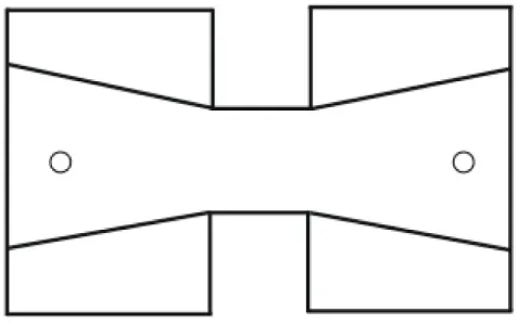 |  |
| Second-order visibility graph (architecture) | Observation location | Overlap of locations’ viewsheds | Directed or undirected | 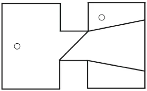 | |
| Visibility graph (landscape) | Observation location | Intervisibility of locations | Directed or undirected | 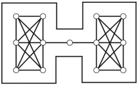 |  |
Summary of multi-disciplinary overview of network data representation for visual relational phenomena.
Visibility Graph (Architecture)
In a visibility graph in the context of architecture, nodes represent isovists/viewsheds and edges represent intervisibility of isovists/viewsheds (Turner et al., 2001). A viewshed or “isovist is the set of all points visible from a given vantage point in space and with respect to an environment” (Benedikt, 1979, p. 47), and it can therefore be considered a visual property of the vantage point. The intervisibility of viewsheds can be defined in two ways: a first-order visibility relationship exists when the viewsheds of a pair of observation locations intersect and if these observation locations are themselves intervisible and a second-order visibility relationship exists when the viewsheds of a pair of observation locations intersect but the locations are themselves not intervisible (Turner et al., 2001). Although it is argued such networks can subsequently be studied with a wide range of graph theoretical measures (Turner et al., 2001, p. 109), the published use of such measures is largely restricted to node clustering coefficient, node neighborhood size, and the mean shortest path length (Batty, 2001; Turner et al., 2001). The neighborhood size of a node is the set of nodes it is directly connected to (its degree in network science terms) and in visibility graphs it represents the number of locations directly visible from an observation location. A node’s clustering coefficient is the number of edges between nodes in its neighborhood divided by the maximum number of edges in a neighborhood of this size and is interpreted as indicating “how much of an observer’s visual field will be retained or lost as he or she moves away from that point” (Turner et al., 2001, p. 110; this interpretation is contested by Llobera, 2003, pp. 27–28). A node’s mean shortest path length is defined as the mean of all shortest paths from this node to all other nodes (what Turner and colleagues refer to here is known in network science literature as a node’s closeness centrality, whereas the mean shortest path length is more commonly used to refer to the mean of all shortest paths between all nodes as a measure for the network as a whole). Batty (2001) further explores the distance attribute of lines-of-sight in a visibility graph, by measuring the average, minimum and maximum distance of a location’s viewshed, as well as the compactness (average divided by maximum distance).
Visibility Graph (Landscape)
Crucial in the context of this paper is that first-order visibility graphs have been proposed for landscape visibility analysis (De Floriani et al., 1994; Nagy, 1994; Puppo and Marzano, 1997; O’Sullivan and Turner, 2001). An overview of the applications of landscape visibility analysis that can be represented by visibility graphs is offered by Nagy (1994), who distinguishes between: locating observation points and hiding places, determining line-of-sight communication networks, scenic and hidden surface paths, identification of landforms like peaks and pits, and the use of visibility for navigation. De Floriani et al. (1994) used visibility graphs to represent lines-of-sight between locations in a landscape, to study the line-of-sight network problem of finding the minimum number of nodes, which must be placed on a landscape to ensure communication through intervisibility between a set of nodes. O’Sullivan and Turner (2001) used the visibility graph as a network data representation of a total viewshed in a landscape (i.e., lines-of-sight from every location to every location in a landscape; Llobera, 2003), and measured the node degree, node clustering coefficient, and the network’s mean shortest path length. The authors suggested visibility graphs could be studied using a wider range of network science approaches, like centrality, cohesive subgroups, and structural equivalence. Such studies are still to appear to our knowledge, and the current paper significantly expands the network science arsenal for studying visibility networks with a different range of techniques closely tied to the theoretical motivations why one creates a visibility network.
Visibility Network Studies in Archeology
Although formal visibility studies in archeology are well established (Lake and Woodman,
2003; Llobera,
2003), visibility network studies in archeology are rare and employ a similarly limited range of network science techniques, often restricting the study to a network diagram representation that is explored visually. An early example is David Fraser’s (Fraser,
1980,
1983, pp. 379–387) study of past power relationships of dominance and subservience, which Fraser argues might be expressed in the dominant and intervisible positions of chambered cairns in Orkney (United Kingdom):
If one cairn can be seen from many other cairns then it is always present and can never be ignored by the users of those other cairns. If messages were passed between cairns by visual means (such as flags or beacons) then a highly intervisible cairn becomes an important link in the dissemination of information (Fraser, 1983, 380).
Intervisibility of cairns was determined through observation in the landscape, reciprocity (i.e., mutual visibility) between cairns was assumed, and a visibility network was created where nodes represent chambered cairns and undirected edges represent intervisibility. Three network measures were applied: the connectivity index refers to the proportion of observed edges over the number of potential edges (i.e., the network density), nodality refers to the degree of a node and degree distribution is explored, and a node’s cutpoint index refers to the number of components created by the removal of this node (Fraser, 1980). Although Fraser concluded the approach did not offer strong evidence for the existence of power relationships expressed through cairn location, it did suggest that certain groups of cairns may have been purposefully located in visually dominant places.
Another example of the creation of visibility networks through observation and visual assessment is provided by Christopher Tilley (1994) (pp. 156–166) in his book “A Phenomenology of Landscape”. An undirected visibility network is explored visually and using node degree, and a process is suggested to explain the patterns identified. This work will be discussed in more detail and expanded on in a brief case study below.
Ruestes Bitrià (2008) in her work on intervisibility of Iron Age hillforts in Catalunya derives a visibility network by representing hillforts as nodes and their intervisibility as edges. The resulting network was explored visually, and it was concluded that it could have supported a communication network. Through his study of hilltop features around the site of Paquimé (Mexico), Swanson (2003) also aimed to explore whether these locations could have functioned as a fire-signaling communication network. An undirected visibility network was created where nodes represent sites and edges their intervisibility. Swanson also compared the visibility network he observed with simulated visibility networks by sampling random points in the landscape, an approach also taken by Earley-Spadoni (2015) in her study of Early Iron age and Urartian fire beacon signaling network. A further study of visual signaling networks is provided in Shemming and Briggs’ (Shemming and Briggs, 2014) analysis of Anglo-Saxon place names and communication networks in Southern England. Possible beacon locations were conjectured from Anglo-Saxon place names, and compared with patterns of intervisibility to explore whether they could indeed serve as a communication network, therefore adding credibility to their identification as beacon locations.
De Montis and Caschili (2012) perform a formal visibility network analysis in their study of intervisibility among Nuraghes (prehistoric towers) in Sardinia (Italy). The authors aim to “investigate the hypothesis that the spatial patterns of the Nuraghes obey rules of intervisibility control over the surrounding territory” (De Montis and Caschili, 2012, 315), that they could have functioned as a communication network, and that they were not isolated entities but worked as a “networked settlement” linked together by lines of intervisibility. The intervisibility network was derived from binary viewsheds using single observer locations on the Nuraghes. Like Ruestes Bitrià and Swanson, the authors also only consider mutual visibility of importance and their network is therefore undirected, missing the opportunity to explore situations where a line of sight between Nuraghes is not reciprocated, which we believe should be included if one wishes to evaluate visual control (we conceptualize visual control as the ability to observe many locations from a vantage point whereas a node’s visual prominence is the ability to be seen from many locations; see Brughmans et al., 2014). Three local node-based measures are used: degree, betweenness centrality and clustering coefficient. The use of betweenness centrality (a measure that calculates paths between nodes which are considered media for the flow of material and immaterial resources) is appropriate in light of the authors’ assumption to treat this network as a communication network.
In her study of settlement patterns in the north-western Dominican Republic, Samantha de Ruiter (2012) aims to evaluate what role visibility could have played in the selection of site locations. De Ruiter emphasizes the need to experience visibility as well as calculate it. Through a survey of the study area the author became familiar with the physical landscape and was able to visually identify key landscape features, resource areas and other sites from site locations, information that was subsequently compared with the results of formal visibility analyses. She calculated the percentage of the study area that is visible from sites and the percentage of sites visible from other sites, which allowed her to create a network of intervisible sites that was explored visually.
Finally, exponential random graph modeling (ERGM) has recently been proposed as an approach to represent and explore the dependence assumptions motivating an archeological visibility study (Brughmans et al., 2014, 2015). The method compares the frequency of configurations (small network patterns representing the dependence assumption) in the observed visibility network with their frequency in stochastic models.
Network Data Representation for Visibility Networks
This overview reveals that network data have been used very differently in a diversity of disciplines to represent a wide range of phenomena. However, there is little cross-fertilization between disciplines in the use of visibility network data representation. A notable exception to this is the use of first-order visibility graphs in both architecture and archeology. We believe that exploring more diverse ways of using network data representations might well lead to useful new ways of studying visibility networks in these and other disciplines. In this section, we will develop this argument for landscape archeology in particular, by offering examples of alternative network data representations of visual properties. To illustrate these examples, we will use the locations of the late pre-colonial sites of Morne Cybèle, Morne Souffleur, and Anse Petite Rivière on the island of La Désirade (Guadeloupe, French West Indies) (we selected these three sites for their prominent locations only to best illustrate the concept of our proposed network methods, an actual visibility study of these sites is published as Brughmans et al., 2017).
In landscape archeology, visibility networks are most commonly created by representing archeological features or sites that are the focus of research interest as nodes, and lines-of-sight between them as undirected edges (Figures
1A,B). However, most sites and features are not single points in space but occupy areas. This can be incorporated in a visibility network in multiple ways:
- (a)
Representing each point location within a site area as a node, and each line-of-sight from each point location as an arc (a directed edge) (Figures 1C,D).
- (b)
Bundling all lines-of-sight of each point location and representing them as a weighted arc (where the weight attribute of the arc represents the number of lines-of-sight) emanating from a single node per site (Figure 1E).
- (c)
Representing the area of a site as a node attribute that can be used in further network analysis (Figure 1F).
- (d)
A combination of the above (Figure 1G).
Figure 1
Representing point locations in site areas as shown in Figures 1C,D offers the advantage of being able to address different questions: from what locations in a site area can locations in another site area be seen? From what locations can other sites not be seen? What locations have both incoming and outgoing lines-of-sight?
Lines-of-sight are commonly represented in landscape archeology as binary undirected edges without attribute information (Figure 1B). However, lines-of-sight in this context are fundamentally directional phenomena, connecting the eyes of an observer with an observed feature. They could therefore be represented as directed arcs (Figures 1E,G), although in many research contexts it is desirable to assume intervisibility when an equal height is used for the observer and target, or due to the limitations of the input data (accuracy of site location, resolution of topography model; see Conolly and Lake, 2006, 230, Figure 10.17). This presents an advantage of network data representations over raster representations of cumulative and total viewsheds in particular, which do not typically distinguish between incoming and outgoing lines-of-sight within a single raster. Instead of binary edges representing either the presence or absence of a line-of-sight between two sites, weighted edges could be used to represent the number of lines-of-sight from all locations in a site area (Figures 1E,G). Finally, additional information about the lines-of-sight, like their length or experimentation settings, could be represented as attribute information of the edge or arc. In research contexts where probabilistic viewsheds are generated (Fisher, 1994), the probability of a line-of-sight could be included as attribute information (e.g., Brughmans et al., 2015). This attribute information can subsequently be used to select and study subnetworks (e.g., all lines-of-sight with a probability over 50% and a length shorter than 3 km).
Network data can also be used to represent phenomena other than direct lines-of-sight between observers and sites, as we have learned from the multi-disciplinary overview in Section “Visibility Network Studies Outside Archeology.” We argue the use of second-order visibility graphs might prove a useful alternative representation of the results of a cumulative viewshed analysis (the locations visible from a set of observation locations; Wheatley, 1995), where a pair of nodes representing sites is connected by an undirected edge if part of the surrounding landscape is visible from both sites (Figure 2). First- and second-order visibility networks allow one to address different research questions. Direct lines-of-sight between sites hypothesized to have formed a signaling network can be explored using a first-order visibility network representation (Figure 2A), whereas the ability to observe the same parts of the surrounding landscape from sites hypothesized to have been used for visually controlling the landscape can be explored using second-order visibility networks (Figure 2B).
Figure 2
Moreover, the use of second-order graphs and landscape visibility graphs can be combined in a two-mode network representation, where one mode represents the observation locations of the cumulative viewshed as nodes and the other mode represents each location in the landscape as nodes. An example of such a two-mode network is shown in Figure 3A, and a geographical representation of the same network in Figure 3B. We purposefully created a visibility network with a very coarse geographical resolution (landscape points are spaced at 200 m intervals), and we want to highlight that this example and the borders of the study area are entirely artificial. This visibility network merely serves to clearly illustrate the method we propose, whereas in real studies an appropriate geographical resolution will need to be selected and the issue of possible edge effects at the borders of the analysis area will need to be addressed. A one-mode projection of this two-mode network on the observation locations results in the second-order graph of observation locations, where a pair of observation locations is connected by a weighted edge representing the number of locations in the landscape they can both observe (Figures 3C,D). A one-mode projection on the landscape locations represents pairs of landscape locations visible from the same observation location (Figure 3E). The two-mode network (Figures 3A,B) has the advantage of allowing one to explore what locations can be observed from what sets of sites, information that is lost in a raster representation of a cumulative viewshed with more than a few observation locations. The one-mode network of observation locations (Figure 3E) offers the advantage of being able to explore clusters of locations that can be observed from the same or similar sets of sites, by using network community detection algorithms (see Fortunato, 2010 for an overview of such methods). Moreover, note how the color coding does not necessarily reflect geographically proximate locations (Figures 3B,D), whereas clusters of nodes with the same color are more clearly visible in this one-mode network representation (Figure 3E).
Figure 3
Finally, we believe landscape visibility graphs could serve as a useful alternative representation of total viewsheds (Llobera, 2003), where each location in a landscape is represented by a node and lines-of-sight connect all intervisible locations. Although much archeological visibility analysis is site-centric by focusing on the visual properties of a set of archeological features, recent studies emphasize the need to study how sites are embedded within the visual properties of landscapes as a whole through the use of total viewsheds: the sum of viewsheds from every single location in a landscape (e.g., Llobera, 2003; Eve and Crema, 2014; Gillings, 2015; Brughmans et al., 2017). In such studies, landscape graphs as introduced by O’Sullivan and Turner (2001) can be used as alternative representations of total viewshed results, in which nodes represent landscape locations and pairs of nodes are connected by an edge if a line-of-sight connects these locations. Figure 4 illustrates this through a purposely coarse resolution total viewshed, to better explain the approach. Both the geographical and network data representations of total viewsheds are useful for highlighting certain patterns, each has distinct advantages over the other. The network data representation does not aim to be as useful in communicating spatial patterns, for which a geographical representation would be more appropriate. We argue these alternative representations can be used alongside each other, applying the most appropriate representation for the data patterns one is interested in. The network data representation of a total viewshed has the advantage of being able to identify structural properties of research interest for a landscape as a whole rather than just for a set of site-based observation locations. Some network measures can be used as alternatives to equivalent measures in a raster data representation of a total viewshed. For example, the degree of a node is equivalent to the number of locations visible from a given raster cell, and the degree distribution is therefore equivalent to the distribution of values in the total viewshed raster. The degree distribution in Figure 5 of the network shown in Figure 4 is skewed to the right, suggesting that most nodes have a limited degree whereas a few have a far higher degree. In this network, the site of Morne Cybèle has the highest degree: it is intervisible with 33 other locations. However, some network science measures have no equivalent in raster data representations and therefore offer new approaches to exploring total viewshed results. Examples include techniques based on the calculation of paths through a network like betweenness centrality, or the node clustering coefficient as proposed for landscape visibility graphs by O’Sullivan and Turner (2001). Of particular interest among these techniques is the ability to identify network data configurations representing theoretical dependence assumptions (see Table 3 for the count of configurations in the network shown in Figure 4). In the next section, we will introduce a range of theoretical dependence assumptions and their associated network data representations that have particular potential for landscape archeology research.
Figure 4
Figure 5
Visibility Theories and Network Patterns
A particularly striking conclusion drawn from the literature above is the limited use, especially in landscape archeology, of network patterns to represent theories about the functioning, emergence, or evolution of visibility networks. Such theories are referred to in network science as dependence assumptions (Brandes et al., 2013): theories about how edges are dependent on each other’s existence. Network patterns can be used as representations of what one expects to see in light of such a theoretical assumption. Visibility theories are often implied in archeological studies of visibility networks and even commonly stated explicitly. For example, in their study of visibility networks among Nuraghes in Sardinia, De Montis and Caschili (2012) hypothesize the existence of a communication network and argue this is reflected through paths in the visibility network. This represents a visibility theory: Nuraghes are positioned in such a way that they are intervisible with other Nuraghes and together create paths, where information can be spread by visual signaling between a pair of not-intervisible Nuraghes through a third. Such theories can be represented by network patterns, commonly called configurations in network science. For example, De Montis and Caschili (2012) consider a path through their visibility network to represent the ability for information to be shared through visible signaling between the Nuraghes.
It is crucial to highlight that the approach we suggest is not concerned with evaluating the probability and reason of the observed network structure emerging in a particular physical landscape. While this would be the ultimate goal, its confounding factors include the underlying social processes, topography, and human interference with it. Instead, we focus on one question only: how likely is it that this observed network is the result of hypothesized structural processes? This assumes that the landscape offers sufficiently many possibilities for the network structure to form, so that it is not necessarily the case that configurations are under- or over-represented. Thus, the model is not restricted by topography and only the hypothesized structural processes are simulated. The abundance of patterns found in simulated networks is then used to assess the significance of those in the observed network.
In Table 2, we list a number of theories drawn from the study of visibility networks in landscape archeology, which could also possibly find useful application in other disciplines. We present undirected network data configurations for these theories, equivalents for directed visibility networks are published by Brughmans et al. (2014).
Table 2
| Configuration | Description | Network pattern |
|---|---|---|
| Isolate | Tendency for nodes to be invisible from other nodes |  |
| Edge | Baseline tendency for pairs of nodes to be intervisible |  |
| Triangle | Tendency for the visibility network to be clustered |  |
| 3-path | Tendency for paths of intervisible nodes. Can be used to represent visual signaling | 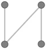 |
| Alternating-star | Tendency for some nodes to have far more lines-of-sight than others, i.e., the degree distribution is spread or skewed. Can be used to represent visually prominent nodes or nodes visually controlling other nodes in the landscape | 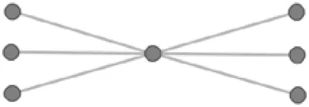 |
Configurations for theories of visibility networks in landscape archeology.
Isolates can be used in studies where the tendency for nodes to be invisible is explored (e.g., Gillings, 2015), while edges can be used to represent a tendency for nodes to be connected in the network. Triangles can be used to represent a tendency for the visibility network to be clustered. Paths can be used to represent communication through intermediary nodes, in studies where visual signaling networks are hypothesized (e.g., Fraser, 1983; De Montis and Caschili, 2012; Ruestes Bitrià, 2008; Swanson, 2003; Shemming and Briggs, 2014): we expect a non-trivial signaling network to contain paths where information can be shared between a pair of non-intervisible locations via one or more intermediary locations. Alternating-stars can be used to represent visually prominent nodes, or nodes visually controlling surrounding nodes, in studies where the importance of hub nodes in the visibility network are hypothesized (e.g., Fraser, 1983; Tilley, 1994). A network with a high number of alternating-stars will have a highly skewed degree distribution, with very few nodes having a high number of links while most nodes have a very limited number of links (for technical details see Koskinen and Daraganova, 2013, 65–67). Moreover, where more geographical reality is desired and appropriate, the length of lines-of-sight can be incorporated in all these network data patterns as an edge attribute to explore correlations between changes in length and probabilities of the creation of network data patterns (for geospatial models including edge length, see Robins and Daraganova, 2013, 99–101).
These network data configurations can be used in a diversity of ways to express and explore theories about the structure and development of visibility networks, and how they affected past human behavior. In the first instance, one can identify those configurations that best express one’s theories. One would expect the configurations representing one’s theories to be particularly frequent in the observed visibility network, which can be evaluated by counting the frequency of all configurations in the network being studied. The first column of results in Table 3 shows the count of configurations of the total viewshed network presented in the previous section (Figure 4): this network has a high number of star configurations, triangles and three-paths, and few isolated nodes.
Table 3
| Configuration | Observed network | Random network | Fixed density | Structural zeroes | Fixed density and structural zeroes |
|---|---|---|---|---|---|
| Nodes | 120 | 120 | 120 | 120 | 120 |
| Edges | 460 | 3,581.422 | 460 | 3,568.37 | 460 |
| Density | 0.064 | 0.502 | 0.064 | 0.499 | 0.064 |
| Isolates | 4 | 0 | 0.0422 | 0 | 0.0415 |
| Triangle | 682 | 35,448.42 | 74.525 | 35,065.17 | 74.576 |
| 3-path | 64,883 | 12,546,873 | 26,411.43 | 12,412,036 | 26,410.529 |
| Alternating-star | 1,416.301 | 13,845.688 | 1,369.571 | 13,793.479 | 1369.547 |
Count of visibility network configurations in the total viewshed network shown in Figure 4 above, and in four different Bernoulli random graph models (10,000 randomly generated networks with 120 nodes).
All counts are averages over all 10,000 samples. Note how comparison of counts of configurations between these networks with strongly different densities is problematic because higher configuration counts can be expected merely due to the higher network density.
However, a simple count of configurations does not reveal whether they are more frequent than would be expected by chance in a network of this size. To evaluate this, we can represent a random process where edges between each pair of nodes are created with equal probability, through a Bernoulli random graph model: each edge will have a probability of being created at the toss of a coin. The count of configurations of the graphs resulting from such a model can be compared with those of the observed network to evaluate whether a random graph model where edges emerge independent of each other is a good description of the observed visibility network. The result of a Bernoulli random graph model with 120 nodes are shown in the second column of Table 3 (the configuration counts are averages over 10,000 randomly generated networks), confirming that the observed network differs strongly from the randomly generated ones, which are far more dense (3,581.422 edges on average, compared to 460 edges for the observed network). Network density is defined as the fraction of the number of edges that are present to the maximum possible number of edges in the network. However, comparison with such randomly generated networks is problematic because they will always have about 50% of all edges present, whereas this is rarely possible for visibility networks in physical landscapes. Comparison of configuration counts between networks with different densities as in Table 3 is problematic, since a higher count can be expected for all configurations in networks with higher network density. We merely included this example of a random network model with network density 0.5 because we noticed this model is very commonly but inappropriately used in archeological and historical network research due to the misleading appearance of unbiased randomness, which is in reality a strong bias toward fixed 0.5 network density. We strongly argue for random network models to assume the same network density as the observed networks they are compared with. In the next section, we will explain why it is more appropriate to compare with a model with network density equal to the observed network.
Density of Visibility Networks in Physical Landscapes
The main reason why randomly generated networks are far denser than the observed visibility network is simply that, combinatorially, there are many more dense networks. An instance sampled uniformly at random from the set of all networks is not subject to limitations imposed by physical realities. However, in real-world physical environments, visibility network density is affected by the maximum viewing distance, observer and target elevation, the spatial density of observation points (points-per-area), the landscape topography, vegetation and atmospheric conditions: in actual landscapes some lines-of-sight between pairs of observation points can therefore never be created, while in randomly generated networks all edges between all pairs of nodes have a probability of being created. In this section, we give a few examples of how much visibility network density can vary in physical landscapes, to illustrate the importance of incorporating visibility network density into visibility network models. The examples are shown in Figures 6–10 and their network density scores are presented in Table 4.
Figure 6
Figure 7
Figure 8
Figure 9
Figure 10
Table 4
| Node distribution | Landscape topography | |||||
|---|---|---|---|---|---|---|
| Flat | Hilly | Mountainous | ||||
| Observer elevation | 1.6 m (Figure 6) | 1.6 m (Figure 7) | 10 m (Figure 9) | 1.6 m (Figure 8) | 10 m (Figure 10) | |
| 36 nodes | Regular | 0.378 | 0.002 | 0.035 | 0.011 | 0.030 |
| Patterned | 0.270 | 0.008 | 0.056 | 0.022 | 0.035 | |
| Random | 0.416 | 0.016 | 0.078 | 0.016 | 0.033 | |
| 100 nodes | Regular | 0.436 | 0.005 | 0.045 | 0.003 | 0.034 |
| Patterned | 0.244 | 0.012 | 0.070 | 0.020 | 0.036 | |
| Random | 0.487 | 0.009 | 0.058 | 0.025 | 0.038 | |
The maximum viewing distance concerns both the effects of the curvature of the earth and the distance at which features of interest are visually distinguishable. In a landscape with flat topography, the higher the observation height and the higher the observed feature, the further this feature will remain visible above the horizon. But inevitably all features become invisible to a human observer as they disappear behind the curvature of the earth, which limits the network density of visibility networks spanning huge areas. Moreover, landscape archeologists are often particularly interested in the ability of human observers to see particular features such as archeological sites, smoke columns, or other humans. This can be affected by the distance at which the feature is physically visible to humans in general, the ability of a particular observer to distinguish the feature (i.e., cultural affinity with the feature, regular exposure to the feature, or the state of the observer’s eyesight), and how the feature contrasts against the background (Wheatley and Gillings, 2000). In such cases, a theoretical maximum distance can be determined up to which features of interest are distinguishable by the observer (e.g., Gillings, 2015). The effect maximum viewing distance has on the network density of visibility networks in a flat landscape is therefore to connect pairs of nodes spaced at distances shorter than the maximum viewing distance and not to connect pairs of nodes at longer distances. This is illustrated most clearly in the patterned distribution shown in Figure 6, where nodes positioned in the four corners of a flat landscape are not intervisible because they are too far away from each other.
However, the examples shown in Figures 7 and 8 caution against generalizing trends in visibility network density derived from unrealistically flat landscapes: visibility network density can be as variable as the landscapes and the observer distributions they are derived from. Figure 7 shows visibility networks in a hilly landscape in Grande-Terre and Figure 8 shows visibility networks in a particularly mountainous landscape in Basse-Terre (both in Guadeloupe, French West Indies). Most obvious is that visibility networks in flat landscapes (Figure 6) are far denser than those in hilly and mountainous landscapes (Figures 7 and 8). Moreover, a higher number and overall spatial density of observation locations (points-per-area) does not necessarily lead to a higher visibility network density, since network density is relative to the number of nodes in the network: the higher the number of nodes, the more edges that need to be created to get a certain network density score. High local spatial densities of observation locations often lead to clusters in the visibility network between closely spaced sets of nodes, but can also lead to lower visibility network densities if these clusters are spaced at distances higher than the maximum viewing distance (see patterned distributions in Figures 6–8). A factor that does clearly lead to higher visibility network densities is higher elevations of observer and target locations (e.g., through the use of observation towers), as shown in Figures 9 and 10 where elevations of 10 m were assumed. We will not address the cases of vegetation and atmospheric conditions here, although they can be expected to further reduce visibility network density through obstruction and limiting maximum viewing distance.
We did not aim to provide a complete overview of visibility network density variability, but merely a range of examples that nevertheless allow for some summarizing remarks. Dense visibility networks can be expected in cases where most observation locations are positioned close to each other (within the maximum viewing distance), observer and target elevations are high, and there is little visual obstruction caused by topography. Sparse visibility networks can be expected in cases where observation locations are positioned far from each other, observer and target elevations are low, and there is much visual obstruction caused by topography.
In landscape archeology research contexts, there can be enormous variety in the spatial density (points-per-area) and distribution of observation points, the theorized maximum viewing distance, and the topography of the research area. However, the archeological literature review presented above revealed that, so far, visibility networks have been mainly used in research contexts where the intervisibility of large features is considered, like site areas, towns, long barrows, or hillforts, that are rather sparsely distributed over large and often hilly to mountainous landscapes and only a single observation point per feature is considered. In such cases, one can expect rather sparse visibility networks if past communities did not consider intervisibility between features in deciding on their locations, and slightly denser networks if features are positioned on great vantage points that offer lines-of-sight to other features. Higher densities can be expected in research contexts where high observation or observed elevations are assumed (e.g., Figures 9 and 10), such as lookout towers or smoke columns, where multiple observation locations would be used throughout site areas (e.g., Figures 1C,D), or where visibility over huge distances can be assumed, such as for the use of fire beacons in visual signaling networks.
The impact on visibility network density of a research context’s particular landscape topography and assumed maximum viewing distance suggests to us that a convincing visibility network model should account for these elements. For example, we could modify the Bernoulli random graph model presented in the previous section in three ways. First, when randomly creating networks the network density can be fixed to that of the observed network. Second, when randomly creating networks we can prevent edges being created between node pairs that are spaced at distances higher than the maximum viewing distance. This can be done by marking these edges as “structural zeroes”: edges that we know cannot possibly exist. Third, the previous two techniques can be combined: a model where the simulated network density is equal to the observed network density, and no edges can be created between nodes farther removed from each other than the maximum viewing distance. Table 3 shows the results for these three techniques applied to the total viewshed visibility network introduced in the previous section: we notice that in this particular case fixing, the network density has a much stronger effect on results since the research area is small and there are few node pairs spaced at distances larger than the maximum viewing distance (i.e., few structural zeroes). However, in all cases, the observed network configuration counts are still very different from those of randomly generated networks. Since this is merely an abstract example to illustrate these techniques, we will not interpret these results any further here but rather apply them in a more interesting archeological case study in Section “Intervisibility of Long Barrows in Cranborne Chase” below.
ERGMs for Visibility Networks
Counts of configurations provide formal descriptions of the visibility networks, but on their own they do not reveal much about the processes giving rise to this network. We can explore such processes by comparing the structural features of the observed network with those of models that represent our archeological theories about the processes governing the creation and evolution of this network. Does a model with a tendency to create paths to enable visual communication and visually prominent nodes but no isolated nodes offer a good description of the observed network? Such questions can be addressed with ERGM, an approach belonging to a family of statistical models originally developed for social networks (Wasserman and Pattison, 1996; Anderson et al., 1999). ERGMs aim to investigate the dependence assumptions underpinning hypotheses of network formation by comparing the frequency of particular configurations in observed networks with their frequency in stochastic models that include selected configurations as effects. This approach applied to the study of visibility networks is described elsewhere (Brughmans et al., 2014), and detailed technical documentation of the ERGM method and all configurations is available (Lusher et al., 2013, and see in particular for geospatial ERGMs including edge length, Robins and Daraganova, 2013, 99–101). We further illustrate the use of ERGMs in the brief case study below.
There are a number of advantages to exploring our theories surrounding visibility networks through stochastic statistical models. First, it provides a formal representation of our archeological theories that facilitate communication as well as formal comparison with visibility networks in other geographical or temporal contexts. Second, our theories are often rather complex, involving multiple effects that can influence each other and cannot be easily derived from merely exploring the structural features of the observed visibility network or even counting the frequency of configurations. Third, a stochastic model introduces a degree of uncertainty resulting in a distribution of possible visibility networks, which is appropriate given the uncertainty inevitably associated with most archeological theories about visibility networks. Fourth, the approach can allow archeologists to discard and refine the theories they formulate by evaluating whether they provide a plausible description of the observed network which is more likely than that the network was merely the result of chance. In the remainder of this paper, we will illustrate this approach by applying it to an early and highly influential example of the archeological use of visibility networks.
Intervisibility of Long Barrows in Cranborne Chase
Christopher Tilley (1994) studied the intervisibility of Neolithic long barrows at Cranborne Chase (United Kingdom) using a network representation in which nodes represent long barrows and edges represent their intervisibility. The network was determined from observations during multiple visits in clear weather conditions during a period of 5 weeks, and when a clear line-of-sight was impossible due to obstructions like buildings or dense woodland. Tilley made observations from locations closeby or inferred them from a map of the landscape’s elevation. Through an evaluation of the presumed past land cover, it is argued that the observed lines-of-sight are similar to, or underestimate, the degree of visibility in the Neolithic, especially for the more prominent barrows: “there is little evidence to suggest that barrows which are prominently sited and intervisible today might not also have been during the period of their initial construction and use” (Tilley, 1994, 157). The network is subsequently explored visually and by comparing node degree. Tilley argues that some barrows were purposefully positioned with reference to visibility and suggests a process as an explanation of the network patterns he identified through exploratory analysis of the observed visibility network. This presents a highly insightful study of a visibility network in an archeological context, of how the network might have evolved and how visibility of long barrows might have structured past human behavior.
In this section, we will show how applying additional network science techniques provide alternative descriptions of this network and the suggested process, which might lead to new insights. We will illustrate how structural features of particular interest can be identified, how we can formally represent the hypothesized process, and explore to what extent it is in fact an appropriate description of the observed visibility network. This case study merely aims to illustrate these methods and it is outside our scope to evaluate and replicate Tilley’s visibility data collection. We therefore use the visibility network from Figure 5.5 in Tilley (1994, p. 156; verified through personal communication with the author) for a secondary analysis. We will discuss each structural feature of the network that was considered of interest by Tilley, and how they can be explored using network science methods.
A first structural feature is a tendency for long barrows on the periphery of the study area to be isolated: “Part of the process of siting barrows in the center of Cranborne Chase was their relationship to other barrows and the Cursus while, on the periphery, a relationship to topographic features of the landscape, rather than to other monuments, appears to have been of paramount significance” (Tilley, 1994, 158). This suggests different processes are responsible for the creation of the network structure in the center and the periphery of the study area. We will therefore focus our study on understanding the structural properties of the center of the study area (for this reason, the isolated peripheral nodes 29, 30, 31, 32, 33, 34, and 39 are excluded from our analyses presented here). This central subnetwork is shown in Figure 11, and the count of configurations and summary statistics are presented in Table 5. We notice this network still has three isolated nodes 14, 38, and 27 at the center of the study area.
Figure 11
Table 5
| Configurations | Observed network | Random network | Fixed density | Network patterns |
|---|---|---|---|---|
| Nodes | 32 | 32 | 32 | |
| Edges | 49 | 247.702 | 49 | |
| Density | 0.099 | 0.499 | 0.099 | |
| Isolates | 3 | 0 | 1.146 | |
| Triangle | 22 | 617.907 | 4.504 | |
| 3-path | 628 | 55,607.46 | 407.347 | |
| Alternating-star | 102.789 | 862.827 | 94.015 | |
Network measures and count of visibility network configurations in the subnetwork at the center of the Cranborne Chase study area shown in Figure 11 above.
An important structural feature for the center of the study area is a difference in the degree of nodes and the components to which they belong: “In general, it is possible to distinguish between (i) those monuments in which visibility was a primary concern in their location, situated on local high points, false crests and skylines and (ii) those in which visibility was not a dominant concern, situated at lower points in the local terrain” … “It is of interest to note that those barrows with the highest degree of intervisibility with others form members of pairs of larger barrow groups” (Tilley, 1994, pp. 158–159). This structural feature is revealed by the degree and connected component measures shown in Table 5. The network consists of two large connected components, referred to by Tilley as the eastern and western groups. In addition to these two, there is a smaller component consisting of four nodes, and three isolated nodes forming their own components. On average, long barrows are intervisible with about 3 other long barrows (see average degree in Table 5). However, when we plot the distribution of the number of lines-of-sight per long barrow then we notice a strong difference between them (Figure 12): the majority have a low degree (the most frequently occurring degree is 1), and a few nodes have a particularly high degree (long barrow 15 is intervisible with 9 other long barrows, long barrow 10 is intervisible with 7 other long barrows).
Figure 12
A further structural feature for the center of the study area is a tendency for nodes to be connected and not be isolated: “Being able to see other barrows from each mound was clearly an important factor in the location of many of them” (Tilley, 1994, p. 158). The network measures in Table 5 reveal that this network has 49 edges and 32 nodes of which 3 are isolated, with a network density of 0.099. This network density score means that about 10% of all possible edges in a network with 32 vertices are present, which is actually quite dense when compared to the densities of example physical landscapes in Table 4. We did after all purposefully focus on a smaller area at the center of Tilley’s study area where the network is particularly dense.
But what do these numbers mean: is this network density higher than expected by chance for a network of this many nodes? To evaluate this, we created a Bernoulli random graph model, simulating 10,000 randomly generated networks with 32 vertices, which provided the network measures shown in the second column of Table 5. By comparing the structural features of the observed network (first column) with those of the randomly created networks (second column), we notice they are very different: the network density in the latter is much higher, triangles, 3-path, and alternating-star are all much more frequent, and there are no isolates. However, we argued above that this high network density is to be expected and that this is not an appropriate comparison. To represent a random network creation process more appropriate for this particular research context, we can fix the network density to that of the visibility network observed by Tilley (we will not use structural zeroes since no theoretical maximum viewing distance is used in Tilley’s original study). The results of this model are shown in the third column in Table 5, and they are much more similar to the observed network than those of the previous model. However, the number of triangles, 3-paths, and alternating-stars are now all quite a bit less frequent than in the observed network. These results suggest that a random network creation process does not describe the observed visibility network very well. Indeed, we do not expect this network to have been randomly created by individuals in the past, but it is crucial that we confirm this before testing more interesting archeological theories. It is important to show that a random network creation model does not offer a good description of the observed network, because this represents the simplest relational assumption: there is no assumption about the dependency between edges. Excluding a random process allows us to explore more interesting and more complex processes. However, if a random network creation process were to offer a good description of the observed network then we would have to conclude that our ability to attach any confidence to a more complex network creation model with dependency assumptions is very limited.
In addition to Tilley’s identification and interpretation of key structural features mentioned above, the author suggests a hypothetical process that could have led to the observed network structure: “One explanation for this pattern might be that sites that were particularly important in the prehistoric landscape and highly visible ‘attracted’ other barrows through time, and sites built later elsewhere were deliberately sited so as to be intervisible with one or more other barrows. In this manner the construction of barrows on Cranborne Chase gradually created a series of visual pathways and nodal points in the landscape” (Tilley, 1994, p. 159).
To represent this theory, we can create a network model where the creation of edges happens respective to the presence or absence of other edges, rather than generating edges independent of one another as we did with the Bernoulli random graph model. This model should include a tendency for edges to be created to nodes that already have a higher degree, which can be represented by the alternating-star configuration. We can add more dependence assumptions to the model to represent the other structural features that Tilley described as important: a tendency to create lines-of-sight (represented by the edge configuration), visual pathways (represented by the 3-path configuration), and clusters or groups of intervisible barrows (represented by the triangle configuration). We estimated an ERGM with the effects shown in Table 6. The results of a goodness-of-fit test are shown in Table 7, suggesting that the model is a rather good fit but not perfect since the triangle parameter has a t-ratio just higher than 0.1 (here we use the criteria by Harrigan (2007) to determine what makes a good fit: estimated parameters in the model should have a t-ratio below 0.1 and all others below 2). With the aim of obtaining a model with an even better fit, we decided to add to the model the tendency for long barrows in this central part of the study area to be intervisible with at least one other long barrow and therefore not be isolated (represented by the isolates configuration). The estimates of this second model are also shown in Table 6 and the goodness-of-fit results in Table 7, this time the model is a perfect fit.
Table 6
| Effects | Estimates | SE | Significant? | GOF t-ratios |
|---|---|---|---|---|
| MODEL 1 | ||||
| Edge | −3.761 | 0.960 | * | −0.056 |
| Triangle | 1.598 | 0.229 | * | −0.013 |
| 3-path | −0.041 | 0.017 | * | −0.043 |
| Alternating-star | 0.607 | 0.415 | −0.060 | |
| MODEL 2 | ||||
| Edge | −7.567 | 2.480 | * | 0.000 |
| Triangle | 1.610 | 0.227 | * | 0.065 |
| Isolates | −2.529 | 1.450 | −0.063 | |
| 3-path | −0.059 | 0.023 | * | 0.000 |
| Alternating-star | 1.913 | 0.921 | * | −0.005 |
Two estimated exponential random graph modeling models with a good fit to the observed visibility network shown in Figure 11 above.
Results are significant if the absolute value of the estimate is at least two times the absolute value of the SE. Goodness-of-fit (GOF) t-ratios should be lower than 0.1 for the effects included in the model; this t-ratio is derived by comparing the observed count of a configuration with those sampled from simulations: t-ratio = (observation − sample mean)/SE.
Table 7
| Effects | t-ratio MODEL 1 | t-ratio MODEL 2 |
|---|---|---|
| Edge | 0.016 | −0.029 |
| 2-star | 0.198 | 0.073 |
| 3-star | 0.426 | 0.302 |
| 4-star | 0.641 | 0.648 |
| 5-star | 0.885 | 1.024 |
| Triangles | 0.107 | 0.013 |
| 4-clique | −0.388 | −0.514 |
| 5-clique | −0.29 | −0.367 |
| 6-clique | −0.193 | −0.214 |
| 7-clique | −0.133 | −0.136 |
| Isolates | −0.405 | −0.006 |
| Triangle2 | −0.215 | −0.309 |
| Bow_tie | −0.068 | −0.04 |
| 3-path | 0.084 | −0.003 |
| 4Cycle | 0.317 | 0.336 |
| Alternating-star | 0.038 | −0.026 |
| AT(2.00) | 0.438 | 0.326 |
| A2P(2.00) | −0.1 | −0.24 |
| AC(2.00) | −0.407 | −0.537 |
| AET(2.00) | 0.065 | −0.044 |
| SD degree dist | 0.694 | 0.505 |
| Skew degree dist | 1.033 | 0.79 |
| Global clustering | 0.181 | 0.093 |
| Mean local clustering | 0.433 | 0.464 |
| Variance local clustering | 0.06 | 0.054 |
Goodness-of-fit t-ratio results for models 1 and 2 presented in Table 6 above.
Effects included in the model shown in bold.
This second model suggests a tendency against long barrows being isolated as was argued by Tilley, although this result should not be over-interpreted since it is not significant. The negative significant edge parameter suggests intervisibility of long barrows occurs relatively rarely, especially if they are not part of triangles and stars. Such a low network density can be expected in geographical networks where nodes are spread over large landscapes with complex topographies: the distance and obstructions might make many lines-of-sight between pairs of long barrows physically impossible (see section 6 above). The positive significant triangle effect suggests a tendency toward clusters of intervisible long barrows, as was argued by Tilley. The positive significant alternating-star parameter suggests a tendency for some long barrows to be intervisible with far more long barrows than others. This is in line with Tilley’s theory that some long barrows might have “attracted” others, that for some long barrows intervisibility was more important than for others, and that some might be located to ensure intervisibility with several existing long barrows in the landscape. This model can therefore not disprove that this process might have been deliberate. However, the negative significant 3-path parameter suggests this process did not create “a series of visual pathways” as argued for by Tilley, although it definitely does create “nodal points” with a higher degree than other long barrows.
Conclusion
Visibility networks have been used to represent a wide range of relational phenomena in disciplines as diverse as archeology, cognitive sciences, architecture, and urban planning. We have argued that there is room for cross-fertilization between archeology and architecture and landscape studies in the use of network data for representing visibility-related phenomena. We proposed a number of new visibility network data representations for landscape archeology: first- and second-order visibility graph representations of total and cumulative viewsheds and two-mode representations of cumulative viewsheds. Through a range of examples, we further explored the variability in visibility network density in physical landscapes, leading us to argue for the need to explicitly incorporate network density in stochastic models of visibility networks. But most importantly, we identified a very restricted use of formal network science measures for describing, exploring, and analyzing visibility networks, and in particular of the representation and study of theories about how lines-of-sight affect each other’s existence (i.e., dependence assumptions).
In this paper, we have focused on the archeological study of visibility networks to suggest methods for the formal study of archeological relational visibility theories. We suggested a range of configurations to represent and study such theories as network patterns, and statistical simulation methods for comparing these theories with the archeologically observed (or inferred) visibility network. Ultimately, these topological network methods shall incorporate geographical constraints, and possibly processes of topographical reshaping. These approaches should always go hand in hand with the critical formulation of relational visibility theories, and results of such formal methods should always be interpreted in light of these theoretical frameworks, addressing issues such the ability of observers to recognize observed features and the temporality of feature creation.
The brief study of Christopher Tilley’s (Tilley, 1994) visibility network of long barrows in Cranborne Chase illustrated many of these methods. Its contribution to Tilley’s study was twofold: (1) to provide a formal representation of the important structural features and the hypothesis describing the evolution of the visibility network formulated by Tilley, which enables replication of results as well as formal comparisons with visibility networks in other research contexts and (2) to statistically evaluate the probability of Tilley’s theory of the visibility network’s creation and evolution. We argue that the methods illustrated here are particularly appropriate in research contexts where particular structural features are inherent to the formulation of theories about visibility networks (like Tilley’s visibility network of long barrows) and provide formal approaches to complement rich contextual studies of how lines-of-sight could have structured past human behavior.
Software
Viewsheds and visibility networks were created in QGISv2.12.1 using the open source Viewshed Analysis plugin v0.5.1 by Zoran Čučković (2016a,b). Configuration counts, Bernoulli random graph models, and ERGMs were performed using PNet (Wang et al., 2009).
Statements
Author contributions
TB and UB: conception and design of work. TB: drafting of work.
Acknowledgments
We thank Christopher Tilley for his support in verifying the intervisibility network of Cranborne Chase used here. We thank Zoran Čučković for the development of his Viewshed Analysis QGIS plugin and his technical support. We thank Viviana Amati for advice concerning ERGMs. We thank the reviewers for their constructive and detailed feedback, and specifically Irmela Herzog for suggesting the color coding used in Figure 3 and helping to improve the presentation of the paper. The work presented here was performed as part of the Caribbean Connections: Cultural Encounters in a New World Setting project, financially supported by the HERA Joint Research Program, and the European Union’s Seventh Framework Programme for research, technological development, and demonstration under grant agreement no 1133; this research is also part of the project NEXUS1492 (http://www.nexus1492.eu/), which has received funding from the European Research Council under the European Union’s Seventh Framework Programme (FP7/2007-2013)/ERC grant agreement no. 319209.
Conflict of interest
The authors declare that the research was conducted in the absence of any commercial or financial relationships that could be construed as a potential conflict of interest.
References
1
AhmadlouM.AdeliH.AdeliA. (2010). New diagnostic EEG markers of the Alzheimer’s disease using visibility graph. Journal of Neural Transmission117:1099–109.10.1007/s00702-010-0450-3
2
AndersonC.J.WassermanS.CrouchB. (1999). A p* primer: logit models for social networks. Social Networks21:37–66.10.1016/S0378-8733(98)00012-4
3
BattyM. (2001). Exploring isovist fields: space and shape in architectural and urban morphology. Environment and Planning B: Planning and Design28:123–50.10.1068/b2725
4
BenediktM.L. (1979). To take hold of space: isovists and isovist fields. Environment and Planning B: Urban Analytics and City Science6:47–65.10.1068/b060047
5
BrandesU.RobinsG.McCranieA.WassermanS. (2013). What is network science?Network Science1:1–15.10.1017/nws.2013.2
6
BrughmansT.de WaalM.S.HofmanC.L.BrandesU. (2017). Exploring transformations in Caribbean indigenous social networks through visibility studies: the case of late pre-colonial landscapes in East-Guadeloupe (French West Indies). Journal of Archaeological Method and Theory1–45.10.1007/s10816-017-9344-0
7
BrughmansT.KeayS.EarlG. (2015). Understanding inter-settlement visibility in Iron Age and Roman Southern Spain with exponential random graph models for visibility networks. Journal of Archaeological Method and Theory22:58–143.10.1007/s10816-014-9231-x
8
BrughmansT.KeayS.EarlG.P. (2014). Introducing exponential random graph models for visibility networks. Journal of Archaeological Science49:442–54.10.1016/j.jas.2014.05.027
9
ConollyJ.LakeM. (2006). Geographical Information Systems in Archaeology. Cambridge, NY: Cambridge University Press. Available at: http://www.loc.gov/catdir/enhancements/fy0665/2006296605-d.html
10
ČučkovićZ. (2016a). Advanced viewshed analysis: a quantum {GIS} plug-in for the analysis of visual landscapes. The Journal of Open Source Software1.10.21105/joss.00032
11
ČučkovićZ. (2016b). Viewshed Analysis v0.5.1 QGIS Plugin. Available at: https://github.com/zoran-cuckovic/QGIS-visibility-analysis.
12
De FlorianiL.MarzanoP.PuppoE. (1994). Line-of-sight communication on terrain models. International Journal of Geographical Information Systems8:329–42.10.1080/02693799408902004
13
De MontisA.CaschiliS. (2012). Nuraghes and landscape planning: coupling viewshed with complex network analysis. Landscape and Urban Planning105:315–24.10.1016/j.landurbplan.2012.01.005
14
Earley-SpadoniT. (2015). Landscapes of warfare: intervisibility analysis of early iron and urartian fire beacon stations (Armenia). Journal of Archaeological Science: Reports3:22–30.10.1016/j.jasrep.2015.05.008
15
ElsnerJ.B.JaggerT.H.FogartyE.A. (2009). Visibility network of United States hurricanes. Geophysical Research Letters36:1–5.10.1029/2009GL039129
16
EveS.J.CremaE.R. (2014). A house with a view? Multi-model inference, visibility fields, and point process analysis of a Bronze Age settlement on Leskernick Hill (Cornwall, UK). Journal of Archaeological Science43:267–77.10.1016/j.jas.2013.12.019
17
FisherP.F. (1994). Probable and fuzzy models of the viewshed operation. In Innovations in GIS: Selected Papers from the First National Conference on GIS Research UK, Edited by WorboysM.F., 161–175. London: Taylor & Francis.
18
FortunatoS. (2010). Community detection in graphs. Physics Reports486:75–174.10.1016/j.physrep.2009.11.002
19
FranzG.MallotH.A.WienerJ.M. (2005). Graph-based models of space in architecture and cognitive science – a comparative analysis. In Proc. 17th Int. Conf. Syst. Res. Informatics Cybern, 30–38.
20
FraserD. (1980). The cutpoint index: a simple measure of point connectivity. Area12:301–4.
21
FraserD. (1983). Land and Society in Neolithic Orkney. BAR British Series 117. Oxford: Archaeopress.
22
GillingsM. (2009). Visual affordance, landscape, and the megaliths of Alderney. Oxford Journal of Archaeology28:335–56.10.1111/j.1468-0092.2009.00332.x
23
GillingsM. (2015). Mapping invisibility: GIS approaches to the analysis of hiding and seclusion. Journal of Archaeological Science62:1–14.10.1016/j.jas.2015.06.015
24
HarriganN. (2007). PNet for Dummies: An Introduction to Estimating Exponential Random Graph (p*) Models with PNet. Available at: http://www.mysmu.edu/faculty/nharrigan/PNetForDummies.pdf
25
HillierB.HansonJ. (1984). The Social Logic of Space. Cambridge: Cambridge University Press.
26
KoskinenJ.DaraganovaG. (2013). Exponential random graph model fundamentals. In Exponential Random Graph Models for Social Networks, Edited by LusherD.KoskinenJ.RobinsG., 49–76. Cambridge: Cambridge University Press.
27
LacasaL.LuqueB.BallesterosF.LuqueJ.NuñoJ.C. (2008). From time series to complex networks: the visibility graph. Proceedings of the National Academy of Sciences of the United States of America105:4972–5.10.1073/pnas.0709247105
28
LakeM.W.WoodmanP.E. (2003). Visibility studies in archaeology: a review and case study. Environment and Planning B: Urban Analytics and City Science30:689–707.10.1068/b29122
29
LloberaM. (2003). Extending GIS-based visual analysis: the concept of visualscapes. International Journal of Geographical Information Science17:25–48.10.1080/13658810210157732
30
LusherD.KoskinenJ.RobinsG. (2013). Exponential Random Graph Models for Social Networks. Cambridge: Cambridge University Press.
31
MallotH.A.FranzM.O.SchölkopfB.BülthoffH.H. (1997). The view-graph approach to visual navigation and spatial memory. In Proc. 7th Int. Conf. Artif. Neural Networks ICANN97, Lausanne, Switzerland.
32
NagyG. (1994). Terrain visibility. Computers & Graphics18:763–73.10.1016/0097-8493(94)90002-7
33
O’SullivanD.TurnerA. (2001). Visibility graphs and landscape visibility analysis. International Journal of Geographical Information Science15:221–37.10.1080/13658810010011393
34
PuppoE.MarzanoP. (1997). Discrete visibility problems and graph algorithms. International Journal of Geographical Information Science11:139–61.10.1080/136588197242437
35
RobinsG.L.DaraganovaG. (2013). Social selection, dyadic covariates, and geospatial effects. In Exponential Random Graph Models for Social Networks, Edited by LusherD.KoskinenJ.RobinsG.L., 91–101. Cambridge: Cambridge University Press.
36
Ruestes BitriàC. (2008). A multi-technique GIS visibility analysis for studying visual control of an Iron Age landscape. Internet Archaeology23.10.11141/ia.23.4
37
RuiterS. de. (2012). Mapping History: An Analysis of Site Locations in the Northwestern Dominican Republic. Unpublished RMA thesis.
38
SchölkopfB.MallotH.A. (1995). View-based cognitive mapping and path planning. Adaptive Behavior3:311–48.10.1177/105971239500300303
39
ShemmingJ.BriggsK. (2014). Anglo-Saxon Communication Networks. Available at: http://keithbriggs.info/AS_networks.html
40
SwansonS. (2003). Documenting prehistoric communication networks: a case study in the Paquimé polity. American Antiquity68:753–67.10.2307/3557071
41
TilleyC.Y. (1994). A Phenomenology of Landscape. Places, Paths and Monuments. Oxford: Berg.
42
TurnerA.DoxaM.O’SullivanD.PennA. (2001). From isovists to visibility graphs: a methodology for the analysis of architectural space. Environment and Planning B: Planning and Design28:103–21.10.1068/b2684
43
TurnerA.PennA.HillierB. (2005). An algorithmic definition of the axial map. Environment and Planning B: Planning and Design32:425–44.10.1068/b31097
44
WangP.RobinsG.PattisonP. (2009). PNet. Program for the Simulation and Estimation of Exponential Random Graph (p*) Models. User Manual. Available at: http://sna.unimelb.edu.au/__data/assets/pdf_file/0006/662865/PNetManual.pdf
45
WassermanS.PattisonP. (1996). Logit models and logistic regressions for social networks: I. An introduction to Markov graphs and p*. Psychometrika6:401–25.10.1007/BF02294547
46
WheatleyD.W. (1995). “Cumulative Viewshed Analysis: a GIS-based method for investigating intervisibility, and its archaeological application,” in Archaeology and Geographical Information Systems: a European Perspective, eds LockG.StančičZ. (London: Taylor & Francis), 171–186.
47
WheatleyD.GillingsM. (2000). Vision, perception and GIS : developing enriched approaches to the study of archaeological visibility. In Beyond the Map: Archaeology and Spatial Technologies, Edited by LockG.R., 1–27. Amsterdam: IOS Press.
Summary
Keywords
visibility networks, signaling networks, landscape archeology, viewsheds, Bernoulli random graphs, exponential random graph model
Citation
Brughmans T and Brandes U (2017) Visibility Network Patterns and Methods for Studying Visual Relational Phenomena in Archeology. Front. Digit. Humanit. 4:17. doi: 10.3389/fdigh.2017.00017
Received
01 February 2017
Accepted
20 July 2017
Published
11 August 2017
Volume
4 - 2017
Edited by
Colin D. Wren, University of Colorado Colorado Springs, United States
Reviewed by
Irmela Herzog, Landschaftsverband Rheinland, Germany; César Parcero-Oubiña, Consejo Superior de Investigaciones Científicas (CSIC), Spain; Jessica Munson, Lycoming College, United States
Updates
Copyright
© 2017 Brughmans and Brandes.
This is an open-access article distributed under the terms of the Creative Commons Attribution License (CC BY). The use, distribution or reproduction in other forums is permitted, provided the original author(s) or licensor are credited and that the original publication in this journal is cited, in accordance with accepted academic practice. No use, distribution or reproduction is permitted which does not comply with these terms.
*Correspondence: Tom Brughmans, tom.brughmans@arch.ox.ac.uk
Specialty section: This article was submitted to Digital Archaeology, a section of the journal Frontiers in Digital Humanities
Disclaimer
All claims expressed in this article are solely those of the authors and do not necessarily represent those of their affiliated organizations, or those of the publisher, the editors and the reviewers. Any product that may be evaluated in this article or claim that may be made by its manufacturer is not guaranteed or endorsed by the publisher.