Aspects of Tempo and Rhythmic Elaboration in Hindustani Music: A Corpus Study

1. Introduction

Recent advances in digital humanities have brought forward aspects of human behavior using large corpora. The focus of current studies in digital humanities lies largely on language and social data corpora while music corpora have received less exploration. Performance analysis of music corpora can provide us with several insights into different aspects of music and show us the contrasts and similarities between music theory and practice. Such analyses on larger corpora can yield us additional insights that are often difficult to obtain with traditional manual analysis.

Corpus studies are in general driven by the common motivation of contributing empirical results that improve the understanding of a specific property of data in the corpus. In music, typically, these properties are melody, harmony, and rhythm. Manual analyses of such properties in music corpora have been performed as long as the related disciplines, such as ethnomusicology or music theory, have existed. A complete corpus of compositions by Palestrina was analyzed as early as 1920 (Jeppesen and Hamerik, 1946), and a corpus of recordings of Indian music was analyzed by Abraham and von Hornbostel (1904). However, in the last decades, the availability of computational methods enables the evaluation of larger amounts of data more easily. Data-driven analysis of large corpora is especially amenable to computational methods and can provide additional tools for statistical analysis. Such analyses can provide broad corpus level inferences for a musicologist, complementing a manual detailed analysis of small set of representative pieces.

Before answering research questions that can be approached in a corpus study, the needed material needs to be compiled. Serra (2014) discusses the value of developing corpora of music from various cultures and describes central criteria for their development. Within the CompMusic¹ project, methods for the analysis of five specific music cultures were developed, and Serra (2014) introduces the corpora that were compiled for the evaluation of these tools. The criteria for the compilation are motivated by the need to use the corpora for the evaluation of computational analysis methods. While the project focused on corpora of audio recordings, the article provides basic guidelines for the design of music corpora for research in general. Kroher et al. (2015) present a corpus of Spanish Flamenco music. They adopt the criteria as developed by Serra (2014) and compile a corpus of 95 h of audio recordings, along with metadata regarding artist and style. For smaller subsets of these data, they compile vocal melody transcriptions, annotations of melodic patterns, and style families. The presented case studies comprise, for instance, the tonality and tempo related properties of certain flamenco styles in the corpus.

In this article, we base our analyses on a corpus that emerged using the guidelines as presented by Serra (2014). We demonstrate how a corpus that originally targeted development in audio processing can be applied to the analysis of structures in music performances, with results relevant to research in the musicologies and digital humanities.

1.1. Recent Work

The recent work in the context of corpus studies can be roughly divided into symbolic and audio based studies. While the former use some form of manually obtained symbolic representation of music, such as notes in a MIDI file or a sequence of chord symbols, the latter use the audio signal of a music recording as the primary item in the corpus and arrive at insights using signal processing techniques. We will provide an overview of recent corpus studies of melody, harmony, and rhythmic aspects.

Conklin and Anagnostopoulou (2011) aimed at detecting melodic patterns in a corpus of Cretan folk song notations. They documented patterns that are characteristic for specific dances or specific regions. They arrived at their pattern discovery by assuming that interesting patterns are those that occur frequently in a certain target class, but less frequent in an anti-corpus distinct from that target. In a corpus study of Ethiopian lyre, Conklin et al. (2015) refined the methods further to work when no specific anti-corpus is available that helps to define what a pattern of interest could be. Volk and van Kranenburg (2012) determined melodic features that were used to classify Dutch folk songs into tune families. To this end, a subset of a corpus with 2,500 song transcriptions was used, and experts were asked to rate melody pairs in terms of similarity regarding melodic contour, rhythm, and other aspects. They found that the classification into tune families is based on a consideration of multiple characteristics, with characteristic motifs and the overall rhythmic structure playing the most important role. van Kranenburg and Janssen (2014) further elaborated on what research questions could be addressed with a larger corpus of transcribed folk song melodies. Research questions were located in the areas of music cognition, musicology, and music information retrieval. van Kranenburg and Karsdorp (2014) provide one example of such an analysis, which finds and categorizes typical cadences in folk songs in a larger notated corpus.

Starting from audio, Frieler et al. (2016) performed manual mid-level annotations on a large set of Jazz solo recordings. These annotations have an average length of about 2 s throughout the corpus and represent meaningful categories within the jazz genre. They discovered the frequency of mid-level unit types through several stylistic periods and analyzed their motivic relations. The perspective of a more fine grained analysis of signal features such as the intonation was specified as a step of their future work. In the most recent step of their work (Abeßer et al., 2017), they proposed algorithms that extract pitch contours by taking into account the available information from the notation of a performance. They demonstrated how tuning deviations developed over time and were able to assign intonation as a characteristic to a specific musician, and not to style. They focused on the global distribution of signal characteristics, while detailed analyses of temporal development of, e.g., intonation in a specific solo was not at the focus of the article.

Harmonic progressions in 100 rock songs from five decades were analyzed by de Clercq and Temperley (2011). They manually annotated the chord progressions for each song and illustrated the important role of the IV-chord, as well as the historical change that manifests itself in an increasing diversity of chords in later decades. Gauvin (2015) documented the increase of flat-side harmonies in popular music from 1958 until 1971. This result is obtained from manual harmonic transcriptions of 292 songs from that period. Rohrmeier and Cross (2008) analyze 386 Bach chorales in MIDI format and document harmonic characteristics of compositions, such as the asymmetry of chord transitions. They show that few elements govern most of the musical structure, and due to the large number of samples they are able to demonstrate that the n-grams that model the progressions follow a specific distribution. Weiß et al. (2016) addressed the problem of visualization of harmonic development based on audio signal processing techniques and present a case study of analyses of Wagner operas. They arrived at the conclusion that an audio based analysis can provide very helpful visualizations and can guide the interpretation of structures in large amounts of recordings.

Several corpus analysis studies address rhythmic aspects, which are the focus of this article as well. Volk and de Haas (2013) did a corpus-based study on ragtime music. Using a corpus of several thousand MIDI files, they tracked the development of syncopation patterns throughout a period of several decades that is covered by the corpus. Another study with focus on syncopation was performed by Huron and Ommen (2006), who document the development of syncopation in American popular music in periods until 1939. They manually transcribed audio examples and conducted further analyses on the symbolic level and observed an increase in the amount of syncopation throughout this period. Mauch and Dixon (2012) analyzed 4.8 million bar-length drum patterns, extracted from MIDI files. They applied statistical methods from natural language processing by treating the patterns analogously to words, this way predicting the size of the vocabulary of patterns in a corpus. In contrast to speech, they detected high amounts of repetition due to the chosen nature of the corpus. Palmer and Krumhansl (1990) studied how the frequency of note onsets is related to metrical accent in a corpus of Eurogenetic piano compositions. They concluded that the frequency of events corresponds to the strength of metrical accent. Holzapfel (2015) studied rhythmic aspects of a corpus of Turkish makam music in MIDI format, in terms of how the note positions interact with the underlying rhythmic mode. Differences to the distribution of notes in Eurogenetic music were documented, and historical developments through two centuries were illustrated. In contrast to Palmer and Krumhansl (1990), observed patterns do not simply correlate with metrical accent for the musical idiom of Turkish makam music. Recently, London et al. (2017) studied a corpus of percussion recordings from Mali, and also documented that the onsets of percussion instruments tend to form stable contra-metrical patterns similar to the findings by Holzapfel (2015). The recordings were annotated with the progression of the metrical cycle, and onsets of the instruments were annotated in a semiautomatic way. By computing histograms of these onsets, they observed that the onset patterns do not correspond to patterns of metrical accent, as it was observed previously for Eurogenetic classical music.

1.2. Aims and Motivation

Hindustani (Hindustāni) music is an art music tradition that has its origins mainly in the northern parts of the Indian subcontinent (northern and central parts of India, Pakistan, Nepal, and Bangladesh), a vast geographic area with diverse cultures that influence the music. It has a long history of performance and continues to exist and evolve in the current sociocultural contexts. It has a large audience and has attracted a large amount of interest from music scholarship, addressing various questions related to this music culture. The presence of a large dedicated audience and of research literature forms a solid basis for studying this music culture from both a musicological and computational perspective.

Studies of Hindustani music in ethnomusicology have involved larger periods of field studies (see for instance, the work by Clayton (2000), van der Meer (1980), or Widdess (1994)). Many of these studies include the analyses of specific performances, in terms of their structure, melody, or rhythm. As an orally transmitted and mainly improvised music tradition without concrete music scores, performance analyses on audio recordings are valuable for musicological study of Hindustani music. Recent efforts in curating large amounts of digitally available audio recordings of Hindustani music (CompMusic project, see description by Serra (2011)) enables us to perform performance analysis using larger audio corpora. In this work, we focus on an analysis of rhythmic characteristics of Hindustani music.

A number of previous studies focused on Hindustani music corpora. The Bol Processor by Bel and Kippen (1992) aimed to model music with grammars: a formal language representation that emulates tabla drumming. Structures likely to be played can be expressed with the system, but limitations are reached when the complexity of improvisation is taken into account. The system is based on theoretical knowledge, so an interesting question can be how such rules could be derived from a corpus analysis. In particular, influential to the work in this article is the work by Jairazbhoy and Khan (1971), which provided a detailed investigation of melodic (rāg) scale structures. The book does a formal analysis of musical structure by studying a corpus of music, an approach from which we derive our motivation. Perlman (2011) addressed the challenge of the integration of both scalar and melodic processes as an attempt to reconsider the work of Jairazbhoy and Khan (1971), invigorating the so-called “musicological” aspect of ethnomusicology. In this article, we take up an analysis approach to rhythm presented by Jairazbhoy (1983) with the same motivation, to offer a quantitative, musicological perspective on Hindustani music. Hindustani music is primarily an oral tradition, and an analysis of audio recordings of performances can enrich our understanding of musical processes, with statistical analysis over large audio collections yielding general trends of musical traits in the recordings.

With a sizeable annotated corpus of Hindustani music, we can do corpora level analysis of rhythmic characteristics. We provide a detailed description of the corpus and the tempo distribution in the corpus. Further, we focus on a statistical analysis of rhythm and tempo patterns in the Hindustani music corpus. Hindustani music is rhythmically organized within the framework of metrical time cycles called the tāl, with the tāl cycle being the most important metrical structure in Hindustani music. This means that we perform an intra-cycle analysis that aims to present typical rhythmical processes as they occur throughout the duration of a tāl cycle. We present cycle-length descriptions of rhythmic features that facilitate a visualization of which parts of the cycle are commonly emphasized by the percussionists. In addition, we provide descriptions of the typical development of tempo within a metrical cycle.

The corpus content and an analysis of the tempo distribution of the recordings are presented in Section 2. In Section 3, we descend from the presentation of general corpus properties to the analyses of intra-cycle tempo dynamics and rhythm patterns. The obtained patterns describe the general trends in the corpus, and to enrich this abstract level of representation we will proceed to an analysis of specific examples in Section 4. In this step, we will, in collaboration with an expert musician, choose individual examples that are either very typical for the general patterns, or that contradict them. These cases will be analyzed in detail, discussing the musical processes that make the examples either representative or contradicting. These examples can be listened to on the companion webpage of the paper.²

The aim of this study is to showcase the presented methods as a potential application of corpus level analysis, while showing their utility for performance analysis and comparative analysis in musicology. The goal here is to illustrate the possibilities of a corpus level analysis of data, and how such analysis tools can help aid and advance musicology. An example of corpus level musicological analysis is presented here, which amounts to a performance analysis of music in current practice from audio recordings. Our findings generalize the trends documented by Jairazbhoy (1983) on a small set of recordings and provide quantitative aspects on the discussion of typical percussive patterns in Hindustani music.

1.3. Rhythm in Hindustani Music

This section provides the reader with a brief overview of rhythm in Hindustani music. More extensive treatises of the subject are provided by Gottlieb (1993), Dutta (1995), Subhadra (1997), Clayton (2000), Powers and Widdess (2001), Naimpalli (2005), Beronja (2008), and Miron (2011). Gottlieb (1993) contains transcriptions of several Hindustani percussion solos, which can serve as a practical introduction to the subject. Rhythmic aspects in (metered) Hindustani music are based on cyclic metrical structures called the tāl,³ which provide a broad structure for repetition of music phrases, motifs, and improvisations. A tāl has fixed-length cycles, each of which is called an āvart. An āvart is divided into isochronous basic time units called mātrā. The mātrās of a tāl are grouped into sections, sometimes with unequal time spans, called the vibhāgs. Vibhāgs are indicated through the hand gestures of a thālī (clap) and a khālī (wave). The first mātrā of an āvart is referred to as sam, marking the end of the previous cycle and the beginning of the next cycle. The sam is highly significant structurally, with many important melodic and rhythmic events happening at the sam. The sam also frequently marks the coming together of the rhythmic streams of soloist and accompanist, and the resolution point for rhythmic tension (Clayton, 2000, p. 81).

The tempo classes (lay) in Hindustani music can vary between ati-vilaṃbit (very slow), vilaṃbit (slow), madhya (medium), $\text{d}\underset{°}{\text{r}}\text{t}$ (fast) to $\text{ati-dh}\underset{°}{\text{r}}\text{t}$ (very fast). Depending on the lay, the mātrā may be further subdivided into shorter time spans, indicated through additional filler strokes of the tabla. The rhythmic density within the mātrā is referred to as kāl (Stewart, 1974).

There are over 70 different Hindustani tāls described,⁴ while about 20 tāls are performed in regular practice (Clayton, 2000, p. 57). Figure 1 shows four popular Hindustani tāls—tīntāl, ēktāl, jhaptāl, and rūpak tāl, and the structure of these tāls is described in Table 1. The figure shows the sam (marked as ×) and the vibhāgs (indicated with thālī/khālī clap pattern using numerals). A khālī is shown with a 0, whereas the thālī are shown with non-zero numerals. The thālī and khālī pattern of a tāl decides the accents of the tāl. The sam has the strongest accent (with certain exceptions, such as rūpak tāl) followed by the thālī instants. The khālī instants have the least accent.

FIGURE 1

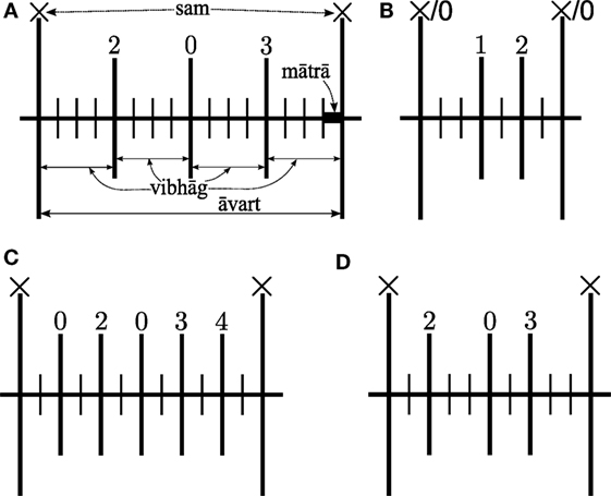
Figure 1. An āvart of four popular Hindustani tāls, showing the mātrās (all time ticks), vibhāgs (long and bold time ticks), and the sam (×). Tīntāl is also illustrated using the terminology used in this article. (A) Tīntāl, illustrated. (B) Rūpak tāl. (C) Ēktāl. (D) Jhaptāl.

TABLE 1

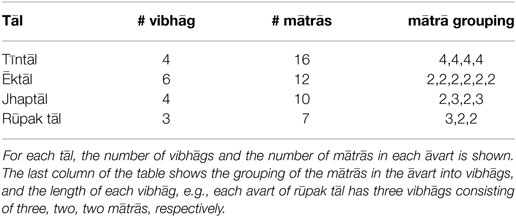
Table 1. Structure of Hindustani tāls.

A jhaptāl āvart has 10 mātrās with four unequal vibhāgs (Figure 1D), whereas a tīntāl āvart has 16 mātrās with four equal vibhāgs (Figure 1A). We can also note from Figure 1B that the sam is a khālī in rūpak tāl, which has 7 mātrās with three unequal vibhāgs. As a special case, ēktāl has six equal duration vibhāgs and 12 mātrās in a cycle as shown in Figure 1C. However, in $\text{d}\underset{°}{\text{r}}\text{t}$ lay, an alternative structure emerges, which is represented as four equal duration vibhāgs of three mātrās each as shown in Figure 2.

FIGURE 2

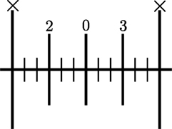
Figure 2. An alternative structure of Ēktāl in $\text{d}\underset{°}{\text{r}}\text{t}$ lay.

Hindustani music uses the tabla as the main percussion accompaniment. It consists of two drums: a left-hand bass drum called the bāyān or diggā and a right-hand drum called the dāyān that can produce various pitched sounds.

Tabla acts as the timekeeper during the performance and indicates the progression through the tāl cycles using predefined canonical rhythmic patterns (called the ṭhēkā) for each tāl. The lead musician (vocal/instrumental) improvises over these cycles, with limited rhythmic improvisation during the main piece. The ṭhēkās are specific canonical tabla bōl patterns defined for each tāl as illustrated in Table 2. The importance of the ṭhēkā in most genres of Hindustani music is such that the tāl tend now to be defined and identified in terms of their ṭhēkā (Powers and Widdess, 2001).

TABLE 2

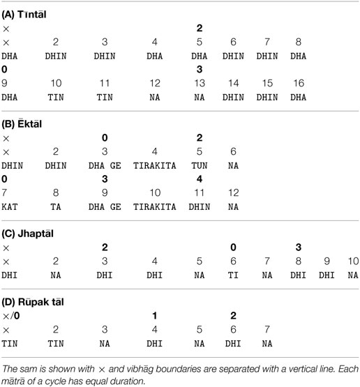
Table 2. The ṭhēkās for four popular Hindustani tāls, showing the bōl for each mātrā.

The strokes of tabla are encoded using onomatopoeic oral mnemonic syllables (bōl). In defining a ṭhēkā, the most important contrast of sonority is between “heavy” and “empty” strokes. The strong heavy strokes comprise an undamped stroke on the left-hand drum, possibly coupled with a right-hand stroke. The light strokes lack the left-hand resonant sound. In the ṭhēkā, heavy strokes are used for the thālī vibhāgs and light strokes for the khālī vibhāgs. However, the correspondence between clap pattern of thālī/khālī and the ṭhēkā are not always so direct. There remains a small number of tāls in which the clap pattern and ṭhēkā bear essentially no relation to each other, e.g., ēktāl and āḍā-cautāl.

In Hindustani music, the tempo is measured in mātrās per minute (MPM). The music has a wide range of tempo, divided into tempo classes called lay as described before. The mainly performed ones are the slow (vilaṃbit), medium (madhya), and fast ($\text{d}\underset{°}{\text{r}}\text{t}$) classes. The boundary between these tempo classes is not well defined with possible overlaps described in different works (Stewart, 1974; van der Meer, 1980; Clayton, 2000). In this article, in correspondence with our coauthor and professional Hindustani musician Kaustuv Kanti Ganguli, we established the following tempo ranges for these classes: vilaṃbit lay for a median tempo between 10 and 60 MPM, madhya lay for 60–150 MPM, and $\text{d}\underset{°}{\text{r}}\text{t}$ lay for >150 MPM. A similar classification into tempo classes was also provided by Stewart (1974) (p. 81). This large range of possible tempi means that the duration of a tāl cycle in Hindustani music ranges from less than 2 s to over a minute. A mātrā in vilaṃbit lay hence can last about 6 s, and to maintain a continuous rhythmic pulse, several filler strokes are played on the tabla. Hence, the surface rhythm emerging from a performance can relate to the underlying metrical structure of the tāl in various ways, a phenomenon that will be illustrated by our results.

In summary, the Hindustani tāls are differentiated not only by length measured in beats, but by the internal organization of the constituent beats. In addition, the musician playing tabla improvises these patterns playing many variations with filler strokes and short improvisatory patterns. Therefore, van der Meer (1980) (p. 93) describes three types of rhythm in Hindustani music: that of the lead soloist, that of the drummer (tabla), and that of the theoretical construct (which is the abstract tāl cycle). In this work, we investigate some relations between the second and the third. The theoretical concepts of tāl, lay and ṭhēkā described so far can have deviations in practice. While the mātrā is defined as isochronous in theory, the tempo in performance varies with expressive timing. In practice, several variations of a typical ṭhēkās can also be performed, and such deviations function to signal approaching cadence or an alternative thematic exposition (Stewart, 1974). These variations provide us a wide variety of rhythm patterns played on the tabla. In this work, we will analyze how the percussion changes depending on the lay, what the tempo dynamics of Hindustani performances are, and, finally, if we can get additional insight into contradictions between the clap/wave patterns and the ṭhēkā variations from our corpus analyses.

2. Hindustani Music Corpus

The corpus used in this article is a subset of the CompMusic Hindustani music collection.⁵ A detailed description of the corpus is discussed by Srinivasamurthy (2016). The collection comprises commercially available music releases from several music labels, artists, and style schools. The subset used in this article will be referred to in the rest of the article as Hindustani Music Rhythm dataset (HMR_f)⁶ (Srinivasamurthy et al., 2016), and it consists of audio excerpts of 2 min length each, annotations that indicate the time positions of the sam and mātrā instances of all performed tāl cycles, and information regarding the lay and tāl of each excerpt. The dataset has pieces from four popular tāls of Hindustani music (Table 3), which encompasses a majority of Hindustani khyāl music. The excerpts include a mix of vocal and instrumental recordings, new and old recordings, and span three lay classes. For each tāl, there are pieces in $\text{d}\underset{°}{\text{r}}\text{t}$ (fast), madhya (medium), and vilaṃbit (slow) lay. All pieces have tabla as the percussion accompaniment. Each piece is uniquely identified using the MusicBrainz IDentifier (MBID) of the recording, which can be used to obtain more information on the origin and form of the recording from the MusicBrainz⁷ database (e.g., artist, release, year, lead instrument, rāg, tāl). The pieces are stereo, 160 kbp, mp3 files sampled at 44.1 kHz.

TABLE 3

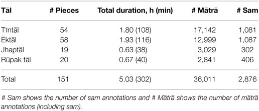
Table 3. HMR_f dataset showing the total duration and number of annotations.

The sam and mātrās annotations were created using Sonic Visualizer by tapping to music and manually correcting the taps, which were then verified by the coauthor Kaustuv Kanti Ganguli, a professional Hindustani musician. Each annotation has a time stamp and an associated numeric label that indicates the mātrā position in the tāl cycle illustrated in Figure 1. The sams are indicated using the numeral 1. The instantaneous tempo of a piece can be obtained from the duration between two mātrā annotations.

The HMR_f dataset is described in Table 3, showing the four tāls and the number of excerpts for each tāl, summing up to 151 excerpts in total. The total duration of audio in the dataset is about 5 h, with 36,011 time-aligned mātrā annotations in a total of 2,876 tāl cycles.

The lay of a piece has a significant effect on rhythmic elaboration in a performance, and to study any effects of the tempo class, the full HMR_f corpus is divided into two subsets. The long-cycle duration subset, HMR₁, consists of a total of 59 vilaṃbit pieces with a median tempo between 10 and 60 MPM, with more than 3,200 mātrā in 300 tāl cycles. A majority of these vilaṃbit pieces are in ēktāl and tīntāl, since it is uncommon for a piece to be performed in vilaṃbit lay jhaptāl and rūpak tāl (there are 6 and 8 pieces for those tāls, respectively, in HMR₁). The short cycle duration subset HMR_s contains the remaining 92 madhya lay (60–150 MPM) and $\text{d}\underset{°}{\text{r}}\text{t}$ lay (150+ MPM) pieces, with over 3 h of audio and more than 32,700 mātrā annotations in 2,572 tāl cycles.

2.1. Tempo Distribution in the Data Corpus

Hindustani music uses a wide range of tempi in performances, and the statistics of tempo distribution over the dataset provides interesting insights to performance. We use the tempo indicators of tāl cycle duration as measured by inter-sam interval τ_s and inter-mātrā interval τ_b as quantities in the analysis. A histogram of the median tempo (computed as 60/τ_b and measured in units of mātrās per minute) of all the pieces in each tāl for HMR_f dataset is shown in Figure 3. These figures show a histogram of the distribution of tempi in the dataset over the whole range of tempi for each tāl. The large range of tempo values and an irregular distribution spanning the whole range is seen with the dataset. The dashed red lines indicate the separators between the tempo classes (dotted line for vilaṃbit to madhya, and dot-dash line for madhya to $\text{d}\underset{°}{\text{r}}\text{t}$).

FIGURE 3

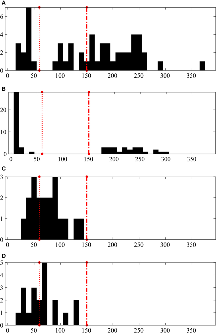
Figure 3. A histogram of the median tempo (in mātrās per minute) in the HMR_f dataset for each tāl. The ordinate is the total number of pieces corresponding to the median tempo value shown in abscissa. The dotted red line and the dot-dash red line indicate the boundaries between the tempo classes (lay) that are used in this article. Note that the y-axis range depends on the number of pieces for each tāl in the dataset. (A) Tīntāl. (B) Ēktāl. (C) Jhaptāl. (D) Rūpak tāl.

From Figure 3, we see multimodal tempo distributions that differ depending on the tāls. We see that tīntāl and ēktāl have the largest tempo range, since they are performed in both slow and fast lay, vilaṃbit and $\text{d}\underset{°}{\text{r}}\text{t}$, respectively. It is remarkable that for ēktāl in Figure 3B the medium tempo range of madhya is basically not present in our corpus. On the other hand, Jhaptāl and rūpak tāl in Figures 3C,D have smaller $\overline{{\mathrm{\tau }}_b}$ ranges, with no examples in $\text{d}\underset{°}{\text{r}}\text{t}$ lay. Both these observations reflect the current performance practices in Hindustani music.

A further consultation with Hindustani musicians and musicologists revealed that the relationship between the lay and tāl depends mainly on the characteristic nature of each tāl, especially the ṭhēkās. The character of the ṭhēkā is tempo dependent and hence specific tāl is preferred to be performed in specific lay. Both jhaptāl and rūpak tāl are medium tempo tāls, and their repertoire is not performed in $\text{d}\underset{°}{\text{r}}\text{t}$ lay. Chakrabarty (2000) also observes that these tāls with non-uniform vibhāg (sections) are best suited for slow to medium tempi where the accent is the most prominent while it is feasible to visualize (vis-a-vis track in working memory) the complete cycle. Ēktāl is popular in both vilaṃbit and $\text{d}\underset{°}{\text{r}}\text{t}$ whereas madhya lay ēktāl performances are rare. Ēktāl has two different vibhāg structures for the different lay ranges of vilaṃbit and $\text{d}\underset{°}{\text{r}}\text{t}$ and hence not performed in medium tempo. Finally, tīntāl ṭhēkā is easily adapted to all tempi and hence it is played in all lay, as we observe in our dataset and the tempo data compiled by Clayton (2000) (p. 84).

In Tables 4 and 5, the statistics of the inter-sam interval τ_s and inter-mātrā interval τ_b are depicted for the long-cycle and short-cycle subsets, respectively. The large range of tempi typical of Hindustani music is reflected in the dataset, with the values of ēktāl cycle lengths ranging from 2.2 to 69.7 s, which is about 5 tempo octaves. Tables 4 and 5 also show that the mātrā period can vary from less than 150 ms to over 6 s. Table 4 shows that the inter-sam interval is largest for ēktāl, indicating that the slow pieces in this tāl take on very low tempi. The other three tāls in the dataset are relatively performed at higher tempi, which is quantified by their smaller cycle durations (Table 4), and their related histograms in Figure 3 not extending as far to the left side as for ēktāl. On the other hand, the statistics of sam and mātrā duration for the short cycle excerpts (HMR_s) in Table 5 quantifies the higher tempo values that both ēktāl and tīntāl can take.

TABLE 4

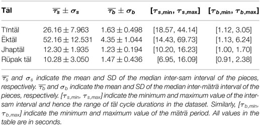
Table 4. Tāl cycle-length indicators for HMR₁ dataset.

TABLE 5

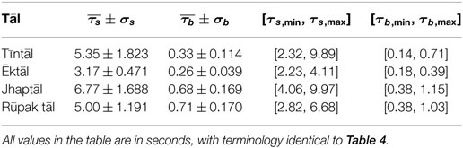
Table 5. Tāl cycle-length indicators for HMR_s dataset.

3. Cycle Level Rhythm Analysis of the Corpus

The āvart (tāl cycle) is the most relevant metrical level in the tāl, and the level around which the whole performance is organized. An analysis on the āvart cycle level will help us to investigate two central aspects in the following two sections of this article. The first aspect is the isochronicity of the mātrā, or, phrased from another perspective, the stability of tempo within a cycle. If deviations from a stable tempo tend to occur at specific mātrā instances of the āvart, this would lead to a prolongation or shortening of certain mātrā. Such a phenomenon has been observed by Jairazbhoy (1983) in a small set of examples, but it has so far not been investigated if it is a consistent performance practice in Hindustani music. The second aspect that our cycle level analysis will approach is a depiction of typical stress patterns that occur in the various tāl, which can be set into relation with the underlying metrical concept of the tāl. These rhythm patterns are computed automatically and are strongly related to the strokes of the percussion instrument.

3.1. Tempo Dynamics

Pieces in Hindustani music are not performed to a metronome, and flexibility in timing leads to what is appreciated by listeners as an expressive performance. Hence an analysis of tempo variations within a cycle of tāl can provide insights into this flexibility, which cannot be obtained by average tempo values as described in Section 2.1.

To analyze the tempo variations within a tāl cycle, we divide the duration from the onset of a cycle to the onset of the subsequent cycle by the number of mātrā in the tāl, with an implicit theoretical assumption that all mātrā in a cycle are equal in duration. This serves as a reference duration for a mātrā that assumes an absolutely stable tempo within a cycle. We then compute the deviation from this value (according to the manual mātrā annotations) for each mātrā in a cycle individually. The average deviation across all cycles for each tāl within a specific subset of the data, i.e., slow or faster tempo classes, is then computed.

Following the suggestion by Jairazbhoy (1983), we use Normalized Units of Time (NUT) to compute the deviation, assuming that the theoretical mātrā duration of the cycle is 100 time units in duration. The deviation at a mātrā position j for a cycle i is computed (in Normalized Units of Time (NUT)) as,

${\mathrm{\Delta }}_j^i=\frac{{\mathrm{\tau }}_b^{\left(i,j\right)}-{\mathrm{\tau }}_b^{\left(i,\ast \right)}}{{\mathrm{\tau }}_b^{\left(i,\ast \right)}}\times 100,$ (1)

where ${\mathrm{\tau }}_b^{\left(i,j\right)}$ is the measured mātrā duration at position j in cycle i, and ${\mathrm{\tau }}_b^{\left(i,\ast \right)}$ is the reference mātrā duration in cycle i with isochronicity assumption. A deviation ${\mathrm{\Delta }}_j^i$ of zero denotes that a mātrā follows exactly the isochronicity assumption. Positive and negative values relate to prolonged and shortened mātrā, respectively. Values that deviate from zero will illustrate the way flexibility of time is shaped by the musicians within the cycle. To the best of our knowledge, for the first time such a characteristic of performance timing will be quantitatively analyzed on a larger set of recordings in Hindustani music.

Figures 4 and 5 show the cycle level deviation in the data subsets HMR₁ and HMR_s datasets, respectively. The figures show the mean deviation (in NUT) of ${\mathrm{\tau }}_b$ and its SD (shown as error bars) from the reference isochronous mātrā period at each specific mātrā position.

FIGURE 4

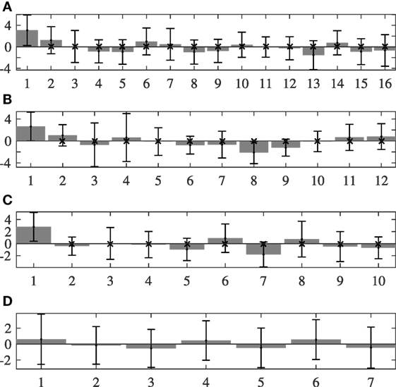
Figure 4. Average deviation ${\mathrm{\Delta }}_{\mathit{\text{j}}}^{\mathit{\text{i}}}$ and its SD (error bars) from the ideal mātrā periods with an isochronous assumption for HMR₁ (long cycle) excerpts. The y-axis shows the deviations in NUT, and the x-axis shows the mātrā position in the cycle. A cross mark at a mātrā position in cycle indicates that the deviation at that mātrā position shows a statistically significant difference to the deviation at the first mātrā of the cycle. (A) Tīntāl. (B) Ēktāl. (C) Jhaptāl. (D) Rūpak tāl.

FIGURE 5

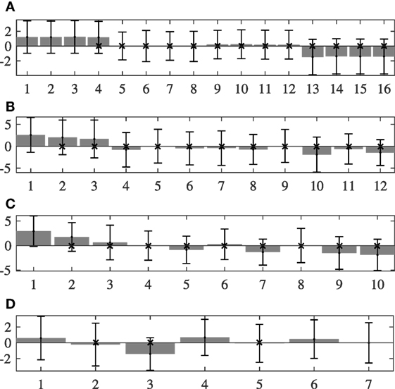
Figure 5. Average deviation ${\mathrm{\Delta }}_{\mathit{\text{j}}}^{\mathit{\text{i}}}$ and its SD (error bars) from the ideal mātrā periods with an isochronous assumption for HMR_s (short cycle) excerpts. The y-axis shows the deviations in NUT, and the x-axis shows the mātrā position in the cycle. A cross mark at a mātrā position in cycle indicates that the deviation at that mātrā position shows a statistically significant difference to the deviation at the first mātrā of the cycle. (A) Tīntāl. (B) Ēktāl. (C) Jhaptāl. (D) Rūpak tāl.

In general, the first mātrā has a positive deviation in τ_b indicating that the first mātrā of the cycle tends to be longer in duration. To assess if this prolongation on the first mātrā is statistically significant compared with the deviations measured at the other mātrā positions in the dataset, we performed a paired-sample t-test between the deviation at the first mātrā and those at every other mātrā position in the cycle. Holm–Bonferroni correction was applied to correct for multiple comparisons. In the figures, a cross at a mātrā position in cycle indicates that the deviation at that mātrā position shows a statistically significant difference (at 5% significance levels) to the deviation at the sam.

From the figures, we observe that rūpak tāl shows a distinct deviation in behavior from the other three tāls, with a more stable tempo at all mātrā positions in both HMR₁ and HMR_s datasets. Apart from rūpak tāl, we observe two different behaviors in other tāls. In the long-cycle pieces of HMR₁, we observe a rather dynamic flexible timing within the cycle (Figure 4). However, with HMR_s dataset, we observe a general trend to speed up from the beginning to the end of the cycle, with the last mātrās being the shortest in duration. The deviations are positive initially in the cycle, while they tend to go negative as the tempo speeds up toward the end of the cycle. This is hypothesized to be due to the tension release at the beginning of the cycle after the sam, while the tension builds up slowly over the cycle as the next sam approaches. This effect is more pronounced in tīntāl (Figure 5A), which shows distinct timing deviations across vibhāgs in HMR_s dataset in contrast to HMR₁ dataset, with the last vibhāg and its mātrās being the shortest and the first vibhāg being the longest. In addition, we also see that the deviations are positive and highest in the first vibhāg, minimal in the second and third vibhāg, and negative in the last vibhāg.

More importantly, we observe that the first mātrā of the cycle right after sam is always the longest, which is attributed to a relaxed timing and release of tension after the sam. For all tāls except rūpak tāl and tīntāl, the average deviation at the first matra also shows statistically significant increase compared with all other positions in both data subsets. For tīntāl, this behavior applies to HMR₁ dataset. With the HMR_s dataset however, interestingly the deviation at the first matra is not significantly different from other mātrās of the first vibhāg while being different from all other mātrās in other vibhāgs. The observations on rūpak tāl are not conclusive, perhaps owing the fewer number of less diverse pieces in the dataset for rūpak tāl.

3.2. Rhythm Patterns

The rhythm patterns are computed using a feature proposed by Böck et al. (2012) for the scope of detecting musical onsets in audio recordings. Since this feature is derived from the time-derivative of the short-time Fourier transform (STFT) magnitude (i.e., the spectrum), it can be referred to as a Spectral Flux feature. Such Spectral Flux features are generally motivated by the fact that the onsets of musical events, such as percussion strokes or a singer intoning a new note, are accompanied by energy increases in certain frequency regions in the spectrum of the signal. The term Spectral Flux expresses this idea of quantifying energy fluctuations in the spectral domain. Furthermore, Spectral Flux features have been successfully applied for the task of automatic meter analysis from audio recordings using rhythm patterns in, e.g., the work by Krebs et al. (2015) and Srinivasamurthy et al. (2015) and hence is a suitable feature for analysis of rhythm patterns.

The process of computing the spectral flux feature is outlined in Figure 6. The short-time Fourier transform (STFT) of the audio signal is computed with a hanning window size of 46.4 ms (first block in Figure 6) and hop size of 20 ms. Subsequently, the resulting frequency bands are grouped using a filter bank with a semitone width, between frequencies from 27.5 Hz to 16 kHz (second block). The differences in time of the logarithmic magnitudes within the obtained 82 frequency bands are then computed, and only positive values are kept (referred to as half-wave rectification in Böck et al. (2012), block 3–4 in Figure 6). The 82 semitone bands are divided into two frequency regions (Low: ≤250 Hz, High: >250 Hz), to obtain a stronger emphasis of the tabla bass drum bāyān in the low region, and an emphasis on the higher-pitched drum dāyān in the high region. Within each of these regions, at each time sample the sum of the frequency coefficients is computed (block 5), and finally a moving average is subtracted to compensate for fluctuations in the energy of the signal (block 6). The output is two Spectral Flux signals, one describing onset energies over time in low frequency, and the other in higher frequency areas.

FIGURE 6

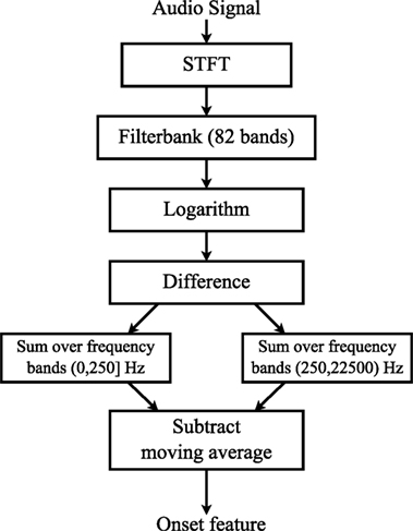
Figure 6. Computation of the spectral flux onset feature in two frequency bands, from Holzapfel et al. (2014).

Starting from the spectral flux feature computed on audio frames, we use the manual time annotations of mātrā on the pieces to extract all cycle-length chunks (sequences) of these features. Since the cycle-length chunks differ in their length depending on the tempo, all cycle-length patterns are interpolated to have the same length, using 32 samples per mātrā. This way, for instance, a cycle-length pattern of tīntāl will have 32 × 16 = 512 samples. We then collect all such patterns within the data subset of interest and compute the average pattern. Since we are interested only in a relative comparison across different positions, the average pattern is then normalized to the range of 0–1. These average patterns represent the amount of energy that is encountered at the individual mātrā for a specific tāl, in average over all the considered pieces. The patterns are indicative of proto-typical surface rhythms present in the audio recordings, and by using the available annotations we can relate these observations to the underlying metrical structure.

The described procedure implies at least to reductions compared with the richness of the original audio material. First, the averaging reduces the diversity of patterns in the individual performances to a single series of numbers. Whereas we will show that such a reduction can provide insights into the relation between performance and underlying concepts, we will in Section 4 take a step back to the specific, and analyze how these average patterns relate to individual performances. And, second, clear and accurate differentiation into various instrumental timbres cannot be achieved using a simple separation into bass and treble frequencies. We will show, however, that some differentiation between the two drums of the tabla can be obtained using this simple procedure.

Figures 7–10 show the cycle-length rhythm patterns for all tāls. We compare rhythm patterns across different lay by plotting the patterns for long-cycle duration HMR₁ dataset (with vilaṃbit lay pieces) and short-cycle duration HMR_s dataset (madhya and $\text{d}\underset{°}{\text{r}}\text{t}$ lay pieces). It is also to be noted that in the HMR_s dataset, $\text{d}\underset{°}{\text{r}}\text{t}$ lay examples are not present for jhaptāl and rūpak tāl while madhya lay pieces of ēktāl are absent. The panel captions of Figures 8–10 reflect this fact. Since tīntāl examples are present in all three lay, Figure 7 illustrates the differences across vilaṃbit, madhya, and $\text{d}\underset{°}{\text{r}}\text{t}$ lay for this tāl.

FIGURE 7

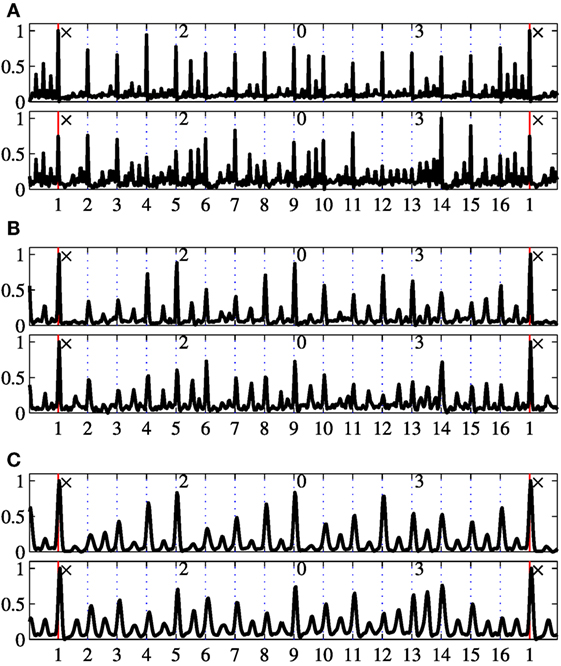
Figure 7. Rhythm patterns for Tīntāl. The panels (A–C) correspond to vilaṃbit, madhya and $\text{d}\underset{°}{\text{r}}\text{t}$ Tīntāl, respectively. In each panel, the lower/upper panes correspond to the low/high frequency bands, respectively. The x-axis shows the mātrā number within the cycle (dotted lines), with 1 indicating the sam (marked with a red line). The y-axis is the normalized amplitude of average spectral flux. The start of each vibhāg is indicated at the top of each pane (sam shown as ×). The plot shows the cycle extended by a mātrā at the beginning and end to illustrate the cyclic nature of the tāl. (A) Vilaṃbit Tīntāl. (B) Madhya Tīntāl. (C) $\text{D}\underset{°}{\text{r}}\text{t}$ Tīntāl.

FIGURE 8

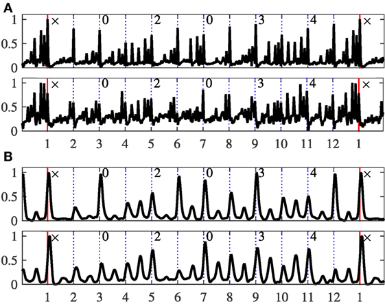
Figure 8. Rhythm patterns for Ēktāl. The axis labels and panels are as described in Figure 7. (A) Vilaṃbit Ēktāl. (B) $\text{D}\underset{°}{\text{r}}\text{t}$ Ēktāl.

FIGURE 9

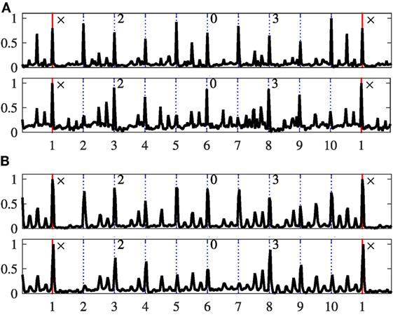
Figure 9. Rhythm patterns for Jhaptāl. The axis labels and panels are as described in Figure 7. (A) Vilaṃbit Jhaptāl. (B) Madhya Jhaptāl.

FIGURE 10

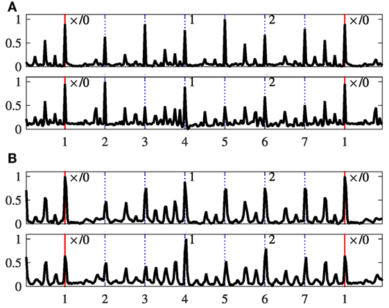
Figure 10. Rhythm patterns for Rūpak tāl. The axis labels and panels are as described in Figure 7. (A) Vilaṃbit Rūpak tāl. (B) Madhya Rūpak tāl.

Within each panel in Figures 7–10, the bottom pane corresponds to the low frequency band, and the top pane corresponds to the high frequency band, respectively. The abscissa is the mātrā number within the cycle (dotted lines), with 1 indicating the sam (marked with a red line). The start of each vibhāg is indicated at the top of each pane (sam shown as ×).

The rhythm patterns in Hindustani music are indicative of tabla strokes played in the cycle, due to the sensitivity of the spectral flux features to fast energy increases over several frequency bands. In the figures, the bottom pane that shows the low frequency band is rather focused on strokes by the bāyān (the left bass drum) of the tabla whereas the top pane focuses rather on strokes from the dāyān (the right pitched drum) of the tabla, but additionally from the lead melody. Hence, for the purpose of this discussion, we use the terms left and right accents to refer to the accents in rhythm patterns from the bottom and top pane, respectively.

The left and right accents provide interesting insights into the patterns played within a tāl cycle. We start from an analysis of the specific patterns that emerged from the individual tāl, and proceed then to a discussion of properties that are shared across all tāl. Some of these observations corroborate the theory while some of them indicate divergence between observed accents and documented ṭhēkā patterns. The analysis and observations discussed in this article were done qualitatively through a visual inspection of the rhythm patterns by the third author in correspondence with other Hindustani music experts. An adequate quantitative comparison of patterns would have required the development of probabilistic measures, for instance an adaptation of the method applied by Holzapfel (2015), which is beyond the focus of this article.

3.2.1. Vilaṃbit tīntāl

From Figure 7A, we see that the 14th mātrā has the strongest left accent, and the last mātrā (mātrā 16) has many filler strokes.⁸ Both indicate the arrival of sam—a phenomenon known as āmad (literal meaning—the approach) (Saxena, 1970). A strong left accent on the 9th matra is not defined in theory while it is observed in the figure. While the stroke in the ṭhēkā at 9th mātrā is a right stroke NA, a DHA is often played instead. This is a known (to practising musicians) difference between theory and practice and can additionally be observed in the patterns too. The right stroke fillers are fewer in mātrās 1 and 2, while the left accents support the timekeeping task. The 4th and 5th mātrā have strong right accents perhaps to indicate the end of the 1st vibhāg, after a (right hand) filler-less mātrās 2 and 3. The beginning of the 2nd and 3rd vibhāgs, labeled 2 and 0, have higher number of fillers. The left accents between the 11th and the 14th matra are particularly weak, with the two right-hand NA strokes clearly standing out in between. The left hand provides stability by subdividing in this phase, with the 11th and 14th mātrā accents acting as anchors for the low-intensity fillers in between them.

3.2.2. $\text{D}\underset{°}{\text{r}}\text{t}$ lay tīntāl

From Figure 7C, we see that the filler strokes in faster tīntāl performances are restricted to a single filler at half mātrā positions in contrast to three or more fillers in vilaṃbit. The accents are more regular due to higher tempi associated. The 11th and 14th mātrās have strong left accents to support the build up of accents through mātrās 12–14 and indicate the arrival of sam (āmad). It is interesting to note that the right accent at vibhāg boundary (mātrā 13) is weaker than that at the previous mātrā 12. This is perhaps due to the stroke on mātrā 13 being skipped and a strong left stroke on mātrā 14 often played to indicate the approaching sam.

3.2.3. Madhya lay tīntāl

In general, Figure 7B shows characteristics, as for instance the density of strokes, that lie between $\text{d}\underset{°}{\text{r}}\text{t}$ and vilaṃbit lay. Some observations of vilaṃbit tīntāl such as a strong left accent on 14th mātrā and on 9th mātrā can also be seen with madhya lay, while the main difference being the presence of less filler strokes. Similar to $\text{d}\underset{°}{\text{r}}\text{t}$ lay, an emphasis is given to right accent on mātrā 12. Mātrā 13 additionally shows a strong right accent indicating that a stroke is played on it in contrast to $\text{d}\underset{°}{\text{r}}\text{t}$ lay, where that stroke is skipped.

3.2.4. Vilaṃbit ēktāl

From Figure 8A, we see that the last matra of the cycle before the sam (mātrā 12) has dense accents, with the final filler strokes having stronger left accents than the sam. This is another example of āmad, where the approach of a sam is distinctly indicated. The mātrās 4 and 10 (both with the ṭhēkā bōl TI RA KI TA, see Table 2) have equal accents in theory. However, mātrā 10 has stronger accents than 4 in practice since it is closer to the sam. TI RA KI TA is often played with more than four strokes toward the end of the matra 4 and 10. Since TI RA KI TA is dense, the mātrā following them (mātrās 5 and 11) have less fillers to distinguish the two mātrā. In addition, only mātrās 4 and 10 have fillers distributed throughout the mātrā, while the rest have fillers only toward the end. Vibhāgs 2 and 3 (spanning mātrās 3–6) and vibhāgs 5 and 6 (spanning mātrā 9-×) are similar in theory, but we can see several deviations in performance, with vibhāgs 5 and 6 having stronger left accents since they are closer to sam. Further, the strokes DHIN at mātrā 1 and mātrā 2 are identical in theory, but in practice the DHIN at mātrā 2 is played softer to differentiate it from the DHIN at the sam. Mātrās 6 and 8 have strong right accents, which relates to the TUN-NA-KAT-TA bols on mātrās 5–8. The modulation of right accent levels through the cycle is interesting, with stronger accents occurring when the mātrā is less dense with lower number of accents. This has a functional role in timekeeping—aided by stronger accents and denser mātrās, which complement each other.

3.2.5. $\text{D}\underset{°}{\text{r}}\text{t}$ lay ēktāl

Though defined with six vibhāgs in theory, $\text{d}\underset{°}{\text{r}}\text{t}$ ēktāl is described better as having four vibhāgs of 3 mātrās each (Figure 2). As can be seen from Figure 8B, the strong right accents due to NA stroke at mātrās 3, 6, 9 and 12 are distinctly seen. This suggests that for $\text{d}\underset{°}{\text{r}}\text{t}$ lay, timekeeping is done more with the sharp right strokes (e.g., “NA” here) and accentuation can even be at non-vibhāg marker mātrās such as 6 and 12. Even though the last vibhāg starts on matra 10, there is a strong right accent on matra 9, an indication of the approaching sam (āmad). The four strokes in TI RA KI TA is often not played in $\text{d}\underset{°}{\text{r}}\text{t}$, replacing it with just two strokes TE KE—we see only two low energy accents in mātrās 4 and 10 since they are played faster. In addition, due to the dense stroke playing on mātrā 4 and 10, the left accents in mātrā 6 and 12 are quiet with relatively weaker accents. Similar to vilaṃbit ēktāl, though the first and second matra have equal accented DHIN stroke in theory, DHIN on the second mātrā is played considerably softer with weak accent. As with all tāls in $\text{d}\underset{°}{\text{r}}\text{t}$ lay, the accents on left and right through the cycle are less differentiated compared with vilaṃbit.

3.2.6. Vilaṃbit jhaptāl

From Figure 9A, we see that all the NA strokes (mātrās 2, 5, 7, 10) have a strong right accent and weak left accents, as described in theory. There are filler strokes to end the vibhāgs at mātrās 2 and 7. This can be explained with the often played variant of the jhaptāl ṭhēkā (DHI NA-TE-KE DHI DHI NA | TI NA-TE-KE DHI DHI NA). There are further strong accented fillers on mātrās 5 and 10 that act as anchor points to indicate the end of half and full cycle.

3.2.7. Madhya lay jhaptāl

Figure 9B shows that the left accents are as defined in theory with basic ṭhēkā playing. In theory, the vibhāg 2 (mātrās 3–5) and vibhāg 4 (mātrās 8–10) are identical, and a similar observation can be seen in performance.

3.2.8. Vilaṃbit rūpak tāl

Rūpak tāl is defined in theory with no left accents on mātrās 1 and 2, but in practice left strokes are often played (with closed and unsustained left strokes). This also implies that rūpak tāl having a khālī (0) on the sam does not mean it is less accented. Rūpak tāl is defined to have a 3 + 2 + 2 structure, but we see from Figure 10A that mātrā 2 has a strong left accent, which acts as an anchor, implying a 1 + 2 + 2 + 2 structure in the vilaṃbit rūpak tāl. This could also be because musicians might play with the same accent on both TIN (mātrās 1 and 2) with a KAT stroke to contrast with the NA stoke which is less left-accented. The vibhāg 2 (mātrās 4–5) and vibhāg 3 (mātrā 6–7) are identical in theory, but in practice the accents differ. Mātrā 5 has the strongest right accent (NA stroke), perhaps indicating āmad. Fillers are more on mātrā 3, to end vibhāg 1. This is due to the often played TI-RA-KI-TA on mātrā 3 (Clayton, 2000). In general, we also see that the fillers get more dense toward the end of vibhāgs.

3.2.9. Madhya lay rūpak tāl

From Figure 10B, the left strokes and accents closely follow the basic bol pattern. The strongest left accent is on mātrā 4, as defined in theory. The vibhāg 2 and 3 are identical with similar accents. In $\text{d}\underset{°}{\text{r}}\text{t}$ rūpak tāl, the accent on the second mātrā is softer than vilaṃbit rūpak tāl, going back to its canonical 3 + 2 + 2 structure compared with 1 + 2 + 2 + 2 structure in vilaṃbit rūpak tāl.

As for general observations, from Figures 7–10, we observe across all tāls and tempo classes that accents are stronger on the mātrās, with less stronger accents present even at several subdivisions of the matra in many cases. The sam most often has the strongest accent. Across all tāls in vilaṃbit lay (Figures 7A–10A), we see additional filler strokes present between mātrās, showing that percussionists add further metrical subdivisions lower than the mātrā. These fillers are concentrated toward the second half of the mātrā. The 1st mātrā (and often the 2nd mātrā) is quite sparse with few accents, while the last few mātrās of the cycle have dense accents. This is to place a special emphasis on the sam, indicating the approaching of sam with fillers and dense stroke playing, while there is a short recovery period after the sam with fewer strokes. In addition, a dense matra with many fillers is often followed by a sparsely accented mātrā to better contrast the progression through the tāl cycle, e.g., a dense mātrā 9 after a quieter mātrā 8 for tīntāl in Figure 7A.

Due to the large mātrā period (${\mathrm{\tau }}_b$) in vilaṃbit lay, each mātrā acts as an anchor for timekeeping and can be played without any effect from the previous strokes (in fast tabla playing in $\text{d}\underset{°}{\text{r}}\text{t}$, the previous stroke can possibly affect the sound, intonation, and playing technique of the following strokes). Further, due to a large time interval available to play the ṭhēkā, the tabla playing musician focuses on modulation of left bass strokes that can sustain longer. Finally, left and right hand can operate independently, which means modulation of accents through the cycle can be different for left and right accents.

By contrast, across all tāls in madhya/$\text{d}\underset{°}{\text{r}}\text{t}$ lay (Figures 7B,C, 8B, and 9B), given the shorter cycles, we see that vibhāgs are anchors. The mātrā subdivisions are largely restricted only to half mātrā, with lower accents and less fillers. In addition, the left and right hands are in sync, which can be seen in the modulation of accents through the cycle being highly correlated between left and right—the left and right strokes work together here, in contrast to complementing each other as in vilaṃbit lay.

4. Analysis of Examples

The previous sections focused on corpus level analysis, with observation on the global level of the whole data corpus. In this section, we provide some illustrative examples from the dataset that help to relate the broad characteristics that were described in the previous sections to specific performances. These specific examples do not necessarily replicate the average observations, but illustrate the deviations that we observe within the corpus.

4.1. Tempo Dynamics: Examples

The specific examples for tempo deviation show one full cycle from a piece in the dataset, highlighting the deviation from the reference mātrā duration with an isochronicity assumption. Figure 11 shows such examples for three different tāl. The bars in the figure at each mātrā position show the deviation in the mātrā duration in NUT.

FIGURE 11

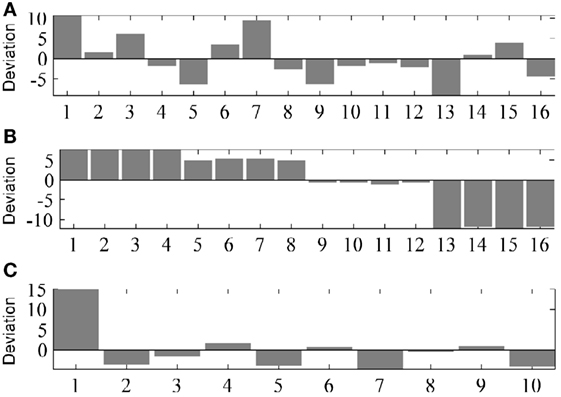
Figure 11. Deviation in mātrā duration over one cycle in three different music pieces. The x-axis shows the mātrā position in cycle, with 1 representing the sam. The bar rectangles show the deviation from the reference mātrā duration with an isochronicity assumption, with the y-axis expressed in NUT. (A) Vilaṃbit tīntāl. (B) $\text{D}\underset{°}{\text{r}}\text{t}$ tīntāl. (C) Vilaṃbit jhaptāl.

Figure 11A shows an example in vilaṃbit tīntāl⁹ showing a higher deviation in first mātrā duration than the average figure depicted in Figure 4A. Figure 11B depicts an example in $\text{d}\underset{°}{\text{r}}\text{t}$ tīntāl¹⁰ that is characterized by a larger tempo decrease in the first vibhāg, and larger tempo increase toward the end of the cycle, compared with the average in Figure 5A. The last example in vilaṃbit jhaptāl¹¹ depicted in Figure 11C is characterized by a first mātrā that is almost 15% longer than expected under a constant tempo assumption. Each of these examples reflects the overall observations from Figures 4 and 5 with some amount of exaggeration. It can be therefore concluded that the average tempo patterns indeed represent a general process that underlies the timing in the performances, with varying emphasis in each performance.

4.2. Rhythm Patterns: Examples

The cycle-length rhythm patterns played in performance are varied, with some patterns being close to the ṭhēkā and some being improvised. Hence the individual cycle-length patterns of a music piece can be widely different from the average patterns discussed in Section 3.2. To assess the similarity of these patterns from the average rhythm patterns, we also compute the similarity of these individual patterns with the average pattern using a correlation based similarity measure. For each rhythm pattern in the dataset, we can hence obtain an estimation of its similarity with the average rhythm pattern for the tāl and the lay it belongs to. A higher correlation for a specific cycle would imply that the pattern being played is similar to the average pattern (as in a basic ṭhēkā), while a low similarity would mean a pattern that is improvised (such as those played during a solo).

In addition, this similarity measure also provides a method for tracking the evolution of rhythm patterns over cycles. The regions where there is significant improvisations would give us lower rhythm similarity measures, while other regions with high similarity measures would indicate patterns closer to average pattern being played. To illustrate this, we present for two examples two consecutive cycles and their rhythm patterns (obtained using spectral flux feature). The examples show how the actually played rhythm pattern changes over consecutive cycles and affects its similarity to the average pattern. Since ṭhēkā variations are more common in faster $\text{d}\underset{°}{\text{r}}\text{t}$ lay pieces, we choose two examples from $\text{d}\underset{°}{\text{r}}\text{t}$ lay.

Figure 12 shows two cycles of a music piece in $\text{d}\underset{°}{\text{r}}\text{t}$ tīntāl,¹² and Figure 13 shows two cycle of a music piece in $\text{d}\underset{°}{\text{r}}\text{t}$ ēktāl.¹³ Both figures plot the spectral flux for two consecutive cycles, plotted one below the other for comparison. In each cycle, the top and bottom panes show the spectral flux in the high and low frequency bands, respectively. The abscissa is the mātrā position in the cycle. The spectral flux for the cycle is shown as a solid line in foreground while the normalized average pattern is shown as a dotted (blue) line in the background. The spectral flux of the current cycle is scaled relative to the average pattern to compare the relative amplitude between the current cycle and average pattern. The figures also show a normalized similarity measure of the cycle with the average pattern as a red line across the plot.

FIGURE 12

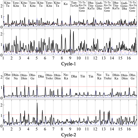
Figure 12. Spectral flux feature for two consecutive cycles of a music piece in $\text{d}\underset{°}{\text{r}}\text{t}$ tīntāl. The x-axis shows the mātrā position in the cycle with vertical dotted lines, and the y-axis is the amplitude of the spectral flux feature. In each figure, similar to Figures 7–10, the top and bottom panes indicate the high frequency and low frequency bands, respectively. The rhythmic pattern for the current cycle is shown as a black solid line in the foreground whereas the blue dotted line in the background indicates the average canonical rhythm pattern for the tāl and lay. The red horizontal line shows the scaled similarity value for the cycle. The tabla strokes played in the cycle are transcribed and shown on the top of the pane.

FIGURE 13

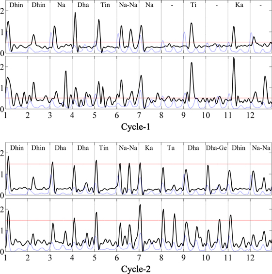
Figure 13. Spectral flux feature for two consecutive cycles of a music piece in $\text{d}\underset{°}{\text{r}}\text{t}$ ēktāl. The colors, axis labels and panels are as described in Figure 12.

In these examples, the spectral flux is higher in amplitude compared with the average pattern, showing that these two examples are characterized by stronger tabla strokes compared with the average. In both these examples, the piece is transitioning from an improvised pattern to an average pattern, and hence we see an increase in similarity measure from Cycle-1 to Cycle-2 (i.e., an increase of the red line). We can also notice the irregular structure of spectral flux in the first cycle, returning to a more regular structure in the second cycle. To verify and illustrate ṭhēkā deviations, a professional musician transcribed the tabla strokes played in both these cycles, which have also been shown for each cycle and example.

In the first example in Figure 12, and we see that the tabla strokes are dense and significantly deviate from the canonical tīntāl ṭhēkā (see Figure 2A) in Cycle-1, while Cycle-2 is more similar to the canonical pattern. This explains the increase in similarity in the second cycle, in which tabla returns from improvised playing back into regular accompaniment style. A similar observation applies for the second example in Figure 13, where the transcription of tabla strokes shows significant deviation from the canonical ṭhēkā of ēktāl (Figure 2B) in Cycle-1. However, unlike a dense stroke playing in the first example, the reason for a lower similarity in first cycle is the deviation in timing and accents: the tabla strokes are played with expressive timing and not on mātrā boundaries.

In each example, the similarity measure tracks actual changes in theka, showing that the average patterns, coupled with a similarity measure, can help to identify and track deviations in patterns played in a music piece over time. This is a useful tool for rhythm analysis of performances, tracking the evolution of rhythm patterns over a whole performance and has the potential to identify improvisatory passages that deviate from the average patterns. The examples in this section served to illustrate that agreement and contradiction between global average observations from large corpora and specific examples. Audio recordings of these examples and additional examples can be seen on the companion webpage at: http://compmusic.upf.edu/corpus-analysis-hindustani.

5. Conclusion

The article presented a rhythm analysis of a Hindustani music corpus, focusing on cycle level tempo dynamics and rhythm patterns. While it is time consuming to manually analyze each recording individually, the corpus analysis methods described here provide us with tools to analyze large corpora and make valuable observations over the entire data. A statistical analysis of the HMR_f dataset showed the wide range of tempi used in Hindustani music performance, and their distribution.

For the first time, an empirical analysis of intra-cycle tempo dynamics was presented for a large Hindustani corpus using the HMR_f dataset. Tendencies observed on specific examples in previous work by Jairazbhoy (1983) could be confirmed and quantified on a larger scale, implying a consistent pattern of expressive timing that emphasizes the internal structure of the underlying metrical cycle. In specific, a significant positive deviation in the duration of the first mātrā of the cycle after the sam was observed (except for rūpak tāl), perhaps implying the release of tension after sam in the first mātrā.

On the other hand, cycle-length rhythm patterns for different tāl and lay in Hindustani music were computed using spectral flux feature, which provided insights about how percussion accents at different positions in the tāl cycle are related to the assumed ṭhēkā. We illustrated the different subdivision strategies depending on tempo, as well as the greater independence of left-hand and right-hand strokes for lower tempi. Finally, a set of concrete set of examples illustrated the structural importance of deviations from these globally averaged tempo and rhythm patterns.

The tools and methods presented in the article show their value for rhythm analysis of large audio music corpora. While the analysis presented needed beat level annotations of audio recordings that are resource intensive if done manually, recent advances in automatic meter analysis methods for Indian art music (Srinivasamurthy et al., 2017) enable us to automatically extract reliable beat level annotations and include large music collections for analysis. We believe that a collaboration with researchers in ethnomusicology could address several questions in more detail, such as the usage of improvised percussion sequences in relation to the overall structure of a performance, or the relation of specific expressive timing characteristics depending on musical style or even individual performer.

Author Contributions

AS, AH, KG, and XS contributed to planning the study and preparing the manuscript. AS and KG contributed to data preparation. AS, AH, and KG contributed to data analysis. AS and AH contributed to writing the manuscript.

Conflict of Interest Statement

The authors declare that the research was conducted in the absence of any commercial or financial relationships that could be construed as a potential conflict of interest.

Acknowledgments

Parts of the article, mainly Section 1.3, Section 2, and Section 3.2 are from the PhD dissertation by Srinivasamurthy (2016). The authors thank Prof. Martin Clayton and Prof. Richard Widdess for their valuable suggestions throughout the process of writing the manuscript. The authors would also like to thank Pt. Ajoy Chakrabarty for the guidance provided in our analysis.

Funding

This work is partly funded by the European Research Council under the European Union’s Seventh Framework Program, as part of the CompMusic project (ERC grant agreement 267583).

Footnotes

1. ^http://compmusic.upf.edu.
2. ^Companion webpage: http://compmusic.upf.edu/corpus-analysis-hindustani.
3. ^Some audio examples illustrating the tāls and structure of more tāls at http://compmusic.upf.edu/examples-taal-hindustani.
4. ^https://www.swarganga.org/.
5. ^http://musicbrainz.org/collection/213347a9-e786-4297-8551-d61788c85c80.
6. ^http://compmusic.upf.edu/hindustani-rhythm-dataset.
7. ^https://www.musicbrainz.org.
8. ^We will refer to energy peaks between the mātrā as “fillers”, since they relate to strokes that fill the temporal gap between the consecutive mātrā by subdividing the mātrā.
9. ^http://musicbrainz.org/recording/0bdad2a8-94d8-40c2-91ec-e77100fcaa02.
10. ^http://musicbrainz.org/recording/35d79f11-0fe5-43ff-97ed-626e2433117f.
11. ^http://musicbrainz.org/recording/a7f28ee8-49af-4572-9c9c-f06b9d85dda2.
12. ^http://musicbrainz.org/recording/cce5404c-de97-4277-9524-a43312337de6.
13. ^http://musicbrainz.org/recording/932be692-9ff8-4fe1-8546-b92b2d3db696.

References

Abeßer, J., Frieler, K., Cano, E., Pfleiderer, M., and Zaddach, W.-G. (2017). Score-informed analysis of tuning, intonation, pitch modulation, and dynamics in jazz solos. IEEE/ACM Transactions on Audio Speech and Language Processing 25:168–77. doi: 10.1109/TASLP.2016.2627186

CrossRef Full Text | Google Scholar

Abraham, O., and von Hornbostel, E.M. (1904). Phonographierte indische Melodien. Sammelbände der Internationalen Musikgesellschaft 5:348–401.

Google Scholar

Bel, B., and Kippen, J. (1992). Modelling music with grammars: formal language representation in the bol processor. In Computer Representations and Models in Music, eds A. Marsden, and A. Pople (Academic Press), 207–238.

Google Scholar

Beronja, S. (2008). The Art of the Indian Tabla. New Delhi: Rupa and Co.

Google Scholar

Böck, S., Krebs, F., and Schedl, M. (2012). Evaluating the online capabilities of onset detection methods. In Proceedings of the 13th International Society for Music Information Retrieval Conference (ISMIR 2012), 49–54. Porto, Portugal.

Google Scholar

Chakrabarty, A. (2000). Shrutinandan. Mumbai, India: Macmillan Publishers India Limited.

Google Scholar

Clayton, M. (2000). Time in Indian Music: Rhythm, Metre and Form in North Indian Rag Performance. Oxford, UK: Oxford University Press.

Google Scholar

Conklin, D., and Anagnostopoulou, C. (2011). Comparative pattern analysis of cretan folk songs. Journal of New Music Research 40:119–25. doi:10.1080/09298215.2011.573562

CrossRef Full Text | Google Scholar

Conklin, D., Neubarth, K., and Weisser, S. (2015). Contrast pattern mining of Ethiopian Bagana songs. In Proceedings of the 5th International Workshop of Folk Music Analysis (FMA), 28–30. Paris.

Google Scholar

de Clercq, T., and Temperley, D. (2011). A corpus analysis of rock harmony. Popular Music 30:47–70. doi:10.1017/S026114301000067X

CrossRef Full Text | Google Scholar

Dutta, A.E. (1995). Tabla: Lessons and Practice. San Rafael, CA: Ali Akbar College.

Google Scholar

Frieler, K., Pfleiderer, M., Zaddach, W.-G., and Abeßer, J. (2016). Midlevel analysis of monophonic jazz solos: a new approach to the study of improvisation. Musicae Scientiae 20:143–62. doi:10.1177/1029864916636440

CrossRef Full Text | Google Scholar

Gauvin, H.L. (2015). “The times they were a-changing”: a database-driven approach to the evolution of harmonic syntax in popular music from the 1960s. Empirical Musicology Review 10:215–38. doi:10.18061/emr.v10i3.4467

CrossRef Full Text | Google Scholar

Gottlieb, R.S. (1993). Solo Tabla Drumming of North India: Its Repertoire, Styles, and Performance Practices. Delhi, India: Motilal Banarsidass Publishers.

Google Scholar

Holzapfel, A. (2015). Relation between surface rhythm and rhythmic modes in Turkish makam music. Journal for New Music Research 44:25–38. doi:10.1080/09298215.2014.939661

CrossRef Full Text | Google Scholar

Holzapfel, A., Krebs, F., and Srinivasamurthy, A. (2014). Tracking the “odd”: meter inference in a culturally diverse music corpus. In Proceedings of the 15th International Society for Music Information Retrieval Conference (ISMIR 2014), 425–430. Taipei, Taiwan.

Google Scholar

Huron, D., and Ommen, A. (2006). An empirical study of syncopation in american popular music. Music Theory Spectrum 28:211–31. doi:10.1525/mts.2006.28.2.211

CrossRef Full Text | Google Scholar

Jairazbhoy, N.A. (1983). Nominal units of time: a counterpart for Ellis’ system of cents. Selected Reports in Ethnomusicology 4:113–24.

Google Scholar

Jairazbhoy, N.A., and Khan, V. (1971). The Rags of North Indian Music: Their Structure and Evolution. London: Faber and Faber Ltd.

Google Scholar

Jeppesen, K., and Hamerik, M.W. (1946). The Style of Palestrina and the Dissonance. Copenhagen: E. Munksgaard.

Google Scholar

Krebs, F., Holzapfel, A., Cemgil, A.T., and Widmer, G. (2015). Inferring metrical structure in music using particle filters. IEEE/ACM Transactions on Audio Speech and Language Processing 23:817–27. doi:10.1109/TASLP.2015.2409737

CrossRef Full Text | Google Scholar

Kroher, N., Díaz-Báñez, J.M., Mora, J., and Gómez, E. (2015). Corpus COFLA: a research corpus for the computational study of flamenco music. ACM Journal on Computing and Cultural Heritage 9:10:1–10:21. doi:10.1145/2875428

CrossRef Full Text | Google Scholar

London, J., Polak, R., and Jacoby, N. (2017). Rhythm histograms and musical meter: a corpus study of Malian percussion music. Psychonomic Bulletin & Review 24:474–480. doi:10.3758/s13423-016-1093-7

CrossRef Full Text | Google Scholar

Mauch, M., and Dixon, S. (2012). A corpus-based study of rhythm patterns. In Proceedings of the 13th International Society for Music Information Retrieval Conference, 163–168. Porto, Portugal.

Google Scholar

Miron, M. (2011). Automatic Detection of Hindustani Talas. Master’s thesis, Universitat Pompeu Fabra, Barcelona, Spain.

Google Scholar

Naimpalli, S. (2005). Theory and Practice of Tabla. Mumbai, India: Popular Prakashan.

Google Scholar

Palmer, C., and Krumhansl, C.L. (1990). Mental representations for musical meter. Journal of Experimental Psychology 16:728–41.

PubMed Abstract | Google Scholar

Perlman, M. (2011). The Rāgs of North Indian music, forty years later. Ethnomusicology 55:318–24. doi:10.5406/ethnomusicology.55.2.0318

CrossRef Full Text | Google Scholar

Powers, H.S., and Widdess, R. (2001). Theory and practice of classical music: Rhythm & tāla. In Grove Music Online. Oxford Music Online, eds S. Sadie, and J. Tyrell, Oxford Music Online, Oxford University Press.

Google Scholar

Rohrmeier, M., and Cross, I. (2008). Statistical properties of harmony in Bach’s chorales. In Proceedings of the 10th International Conference on Music Perception and Cognition, 619–627. Sapporo.

Google Scholar

Saxena, S.K. (1970). The fabric of Amad: a study of form and flow in Hindustani music. Journal of the Sangeet Natak Akademi 16:38–44.

Google Scholar

Serra, X. (2011). A multicultural approach in Music Information Research. In Proceedings of the 12th International Society for Music Information Retrieval Conference (ISMIR 2011), 151–156. Miami, USA.

Google Scholar

Serra, X. (2014). Creating research corpora for the computational study of music: the case of the CompMusic project. In Proceedings of the 53rd AES International Conference on Semantic Audio, London.

Google Scholar

Srinivasamurthy, A. (2016). A Data-driven Bayesian Approach to Automatic Rhythm Analysis of Indian Art Music. Doctoral dissertation, Universitat Pompeu Fabra.

Google Scholar

Srinivasamurthy, A., Holzapfel, A., Cemgil, A.T., and Serra, X. (2015). Particle filters for efficient meter tracking with dynamic Bayesian networks. In Proceedings of the 16th International Society for Music Information Retrieval Conference (ISMIR 2015), 197–203. Malaga, Spain.

Google Scholar

Srinivasamurthy, A., Holzapfel, A., Cemgil, A.T., and Serra, X. (2016). A generalized Bayesian model for tracking long metrical cycles in acoustic music signals. In Proceedings of the 41st IEEE International Conference on Acoustics, Speech and Signal Processing (ICASSP 2016), 76–80. Shanghai, China.

Google Scholar

Srinivasamurthy, A., Holzapfel, A., and Serra, X. (2017). Informed automatic meter analysis of music recordings. In Proceedings of the 18th International Society for Music Information Retrieval (ISMIR) Conference, 679–685. Suzhou, China.

Google Scholar

Stewart, R. M. (1974). The Tabla in Perspective. Doctoral dissertation, University of California, Los Angeles.

Google Scholar

Subhadra, Chaudhary (1997). Time Measure and Compositional Types in Indian Music: A Historical and Analytical Study of Tala, Chanda and Nibaddha Musical Forms. New Delhi: Aditya Prakashan.

Google Scholar

van der Meer, W. (1980). Hindustani Music in the Twentieth Century. London: Martinus Nijhoff.

Google Scholar

van Kranenburg, P., and Janssen, B. (2014). What to do with a digitized collection of western folk song melodies? In Proceedings of the 4th Workshop on Folk Music Analysis (FMA), Istanbul.

Google Scholar

van Kranenburg, P., and Karsdorp, F. (2014). Cadence detection in western traditional Stanzaic songs using melodic and textual features. In Proceedings of the 15th International Society for Music Information Retrieval Conference (ISMIR 2014), 391–396. Taipei, Taiwan.

Google Scholar

Volk, A., and de Haas, W.B. (2013). A corpus-based study on ragtime syncopation. In Proceedings of the 14th International Society for Music Information Retrieval Conference (ISMIR 2013), 163–168. Curitiba, Brazil.

Google Scholar

Volk, A., and van Kranenburg, P. (2012). Melodic similarity among folk songs: an annotation study on similarity-based categorization in music. Musicae Scientiae 16:317–39. doi:10.1177/1029864912448329

CrossRef Full Text | Google Scholar

Weiß, C., Kleinertz, R., and Müller, M. (2016). Möglichkeiten der computergestützten Erkennung und Visualisierung harmonischer Strukturen – eine Fallstudie zu Richard Wagners Die Walküre. In Beitragsarchiv zur Jahrestagung der Gesellschaft für Musikforschung (GfM) 2015 in Halle/Saale, Musikwissenschaft: die Teildisziplinen im Dialog, eds A. Wolfgang, and H. Wolfgang. Available at: http://schott-campus.com/gfm-jahrestagung-2015., Mainz [Schott Campus, urn:nbn:de:101:1-20160912637].

Google Scholar

Widdess, R. (1994). Involving the performers in transcription and analysis: a collaborative approach to dhrupad. Ethnomusicology 38:59–79. doi:10.2307/852268

CrossRef Full Text | Google Scholar