Maximum efficiency control and predictive-speed controller design for interior permanent magnet synchronous motor drive systems

1 Introduction

Interior permanent magnet synchronous motors (IPMSM) have become more and more important due to their high torque per Ampere, good robustness, and high efficiency characteristics (Bose, 2002). IPMSMs have been widely used in home appliances, such as: air conditioners, vacuum cleaners, and lawn mowers. Generally speaking, to save energy and to improve dynamic responses, both a high performance speed controller and high efficiency search algorithms are all required for IPMSM drive systems.

Several researchers have investigated the maximum efficiency control and speed-loop controller designs for IPMSM drive systems. For example, Mahmud et al. investigated an optimum flux searching method for direct torque control of IPMSM drive systems (Mahmud et al., 2020). The relationship between the stator flux linkage and the stator current was analyzed first. Then, a seeking algorithm was investigated to determine the real-time optimal flux and then to generate the maximum torque-per-ampere control. Caruso et al. proposed an experimental investigation of a real-time high efficiency control algorithm for IPMSM drive systems. In that paper, by adjusting the d-axis current, the power losses were changed at varied loads nd speeds (Caruso et al., 2014). Yang et al. proposed efficiency optimization control of IPMSM drive systems, which considered the variations of the motor parameters (Yang et al., 2018). Takaashi et al. studied a high-efficiency control method for an IPMSM drive system by controlling the vector angle of the stator currents (Takaashi and Oguro, 2009). Liu et al. proposed an efficiency-optimal control method for a mono-inverter dual PMSM drive system. A simple optimal efficiency control was proposed. However, the optimal efficiency control was only focused on a dual-PMSM but not a single PMSM (Liu and Fadel, 2018). Kooning et al. investigated the maximum efficiency stator current waveforms for a PMSM and its drive system. The idea was good, however, the stator current waveforms were very complicated, which were difficult to be synthesized (Kooning et al., 2017). Ding et al. used an Artificial Bee Colony algorithm to improve the efficiency of a PMSM-inverter drive system. This algorithm, however, required the losses in the windings and lamination core, which were very difficult to obtain (Ding et al., 2016). Balamurali et al. developed a maximum efficiency control of PMSM drive systems in electric vehicle applications. However, a precise loss model was required (Balamurali et al., 2021). Balamurali et al. proposed a current advance angle to achieve efficiency improvement, which required an efficiency model with experimental tests that were very complicated (Balamurali et al., 2020).

These previously published papers (Ding et al., 2016; Kooning et al., 2017; Liu and Fadel, 2018; Balamurali et al., 2020; Balamurali et al., 2021), however, required an accurate loss model and efficiency model that were obtained by doing a lot of tests. To solve this difficulty, an efficiency control that does not require efficiency model is investigated here. Only the measured or estimated input power and output power are used here. In addition, a predictive speed-loop controller design that improves the transient responses and load disturbance responses is also investigated. To the authors’ best knowledge, the ideas in this paper are original and have not been previously published. This proposed IPMSM drive system can be used for home appliances, such as: air conditioners, vacuum cleaners, and lawn mowers.

2 The interior permanent magnet synchronous motor drive system

Figure 1 shows the block diagram of the proposed IPMSM drive system. The drive system includes two major parts: the hardware circuit and the DSP software. The hardware circuit consists of an inverter, an IPMSM, an encoder, a DC-link voltage, and an A/D converter. The DSP software includes a predictive speed controller, a maximum efficiency control algorithm, a PI current controller, a d-q axis to a-b-c axis coordinate transformation, a space-vector pulse-width modulation (SVPWM), and an a-b-c axis to d-q axis transformation. The whole IPMSM drive system includes two control-loops: a speed control-loop and a current control-loop.

FIGURE 1

FIGURE 1. Block diagram of proposed IPMSM drive system.

2.1 Mathematical model of the interior permanent magnet synchronous motor

Permanent magnet synchronous motors (PMSM) have two major types: surface-mounted permanent magnet synchronous motors (SPMSM) and interior permanent magnet synchronous motors (IPMSM). The IPMSM for this paper is shown in Figure 2. It includes a stator, a rotor, and an air-gap, and it has better robustness, higher operation speeds, and higher total torque than a SPMSM. The d-axis inductance is smaller than the q-axis inductance due to the magnetic salience. Also, because the effective air gap is minimized, the armature-reaction effect becomes clearly and easily noticeable. Furthermore, with a smaller air gap, the flux weakening method is quite effective for the IPMSM.

FIGURE 2

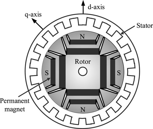
FIGURE 2. Structure of the IPMSM.

Assuming that the input three-phase voltages of the motor are balanced, the d-q axis voltages of the IPMSM are shown as the following equation (Wang et al., 2015):

$\left[\begin{array}{c}{v}_d\\ v_q\end{array}\right]=r_s\left[\begin{array}{c}{i}_d\\ i_q\end{array}\right]+\left[\begin{array}{cc}{L}_d& 0\\ 0& L_q\end{array}\right]\frac{d}{dt}\left[\begin{array}{c}{i}_d\\ i_q\end{array}\right]+{\omega }_e\left[\begin{array}{c}-L_q{i}_q\\ {\lambda }_m+L_d{i}_d\end{array}\right](1)$

where $v_d$ and $v_q$ are the d- and q-axis voltages, $r_s$ is the stator resistance, $i_d$ and $i_q$ are the d- and q-axis currents, $L_d$ and $L_q$ are the d- and q-axis inductances, $\frac{d}{dt}$ is the differential operator, ${\omega }_e$ is the electrical speed, and ${\lambda }_m$ is the permanent magnetic flux linkage of the IPMSM. The total torque of the IPMSM is expressed as follows:

$T_e=\frac{3}{2}\frac{P}{2}\left[{\lambda }_m{i}_q+(L_d-L_q)i_d{i}_q\right](2)$

where $T_e$ is the total torque and p is the pole number. The dynamic speed of the IPMSM is

$\frac{d}{dt}{\omega }_m=\frac{1}{J_t}(T_e-B_t{\omega }_m-T_L)(3)$

where ${\omega }_m$ is the mechanical speed, $J_t$ is the inertia, $B_t$ is the viscous coefficient, and $T_L$ is the torque of the external load. The dynamic equation of the mechanical rotor position ${\theta }_m$ is expressed as follows:

$\frac{d}{dt}{\theta }_m={\omega }_m(4)$

where ${\theta }_m$ is the mechanical rotor position of the IPMSM. The relationship between the electrical rotor position ${\theta }_e$ and the mechanical rotor position ${\theta }_m$ is shown as follows:

${\theta }_e=\frac{P}{2}{\theta }_m(5)$

The relationship between the electrical rotor speed ${\omega }_e$ and the mechanical rotor speed ${\omega }_m$ is depicted as the following equation:

${\omega }_e=\frac{P}{2}{\omega }_m(6)$

2.2 Inverter and space-vector pulse-width modulator modulation method

The power circuit of a three-phase voltage-source inverter is implemented by using six power switches, which are shown in Figure 3A. The power switches can use traditional IGBTs, MOSFETs, or silicon carbide power devices. The power circuit has three independent legs, and each leg includes two power switches–an upper power switch and a lower power switch. For each leg, one power switch is turned on and the other power switch is turned off. When the upper power switch is turned on and the lower switch is turned off, the switching state of this leg is set as “1”. On the other hand, when the upper power switch is turned off and the lower power switch is turned on, the switching state of this leg is set as “0”. For example, if the upper switch of the a-phase is turned on but the upper switches of the b-phase and c-phase are turned off, the switching state of the inverter is expressed as “100”. By using this similar method, one can have six active switching states including 100, 110, 010, 011, 001, and 101, and two zero-voltage switching states including 000 and 111. The details are shown in Figure 3B. In this paper, traditional IGBTs are used.

FIGURE 3

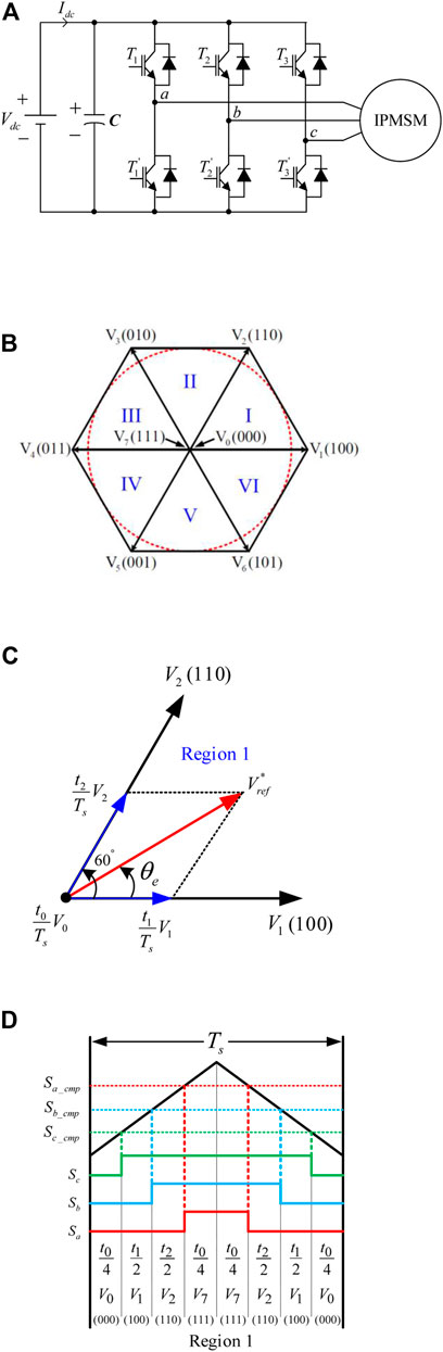
FIGURE 3. The inverter. (A) Main circuit (B) six-step vectors (C) SVPWM (D) turn-on intervals of the a-b-c phase voltages.

The space-vector pulse-width modulation (SVPWM) method in this paper is an advanced, computation-intensive PWM method, which currently might be the best modulation method for variable-frequency AC drive systems. Figure 3C shows the synthesis of the space vector $V_{ref}^{\ast }$. First, if we assume the reference voltage command $V_{ref}^{\ast }$ is in region I, which is shown in Figure 3C, then the reference voltage command is expressed as the following equation:

$V_{ref}^{\ast }=\frac{t_0}{T_s}{V}_0+\frac{t_1}{T_s}{V}_1+\frac{t_2}{T_s}{V}_2(7)$

where $V_{ref}^{\ast }$ is the reference voltage command, $t_0$ is the time interval of the zero voltage vector $V_0$, $t_1$ is the time interval of the active voltage vector $V_1$, $t_2$ is the time interval of the active voltage vector $V_2$, and $T_s$ is the total time interval for one PWM switching cycle. From Figure 3C, according to trigonometric functions, the following two equations are obtained:

$V_{ref}^{\ast }\text{sin}(60°-{\theta }_e)=\frac{t_1}{T_s}{V}_1\text{sin}(60°)(8)$

and

$V_{ref}^{\ast }\text{sin}\left({\theta }_e\right)=\frac{t_2}{T_s}{V}_2\text{sin}(60°)(9)$

From Eqs. 8, 9, one can derive the following three equations:

$t_1=\frac{T_s}{V_1}\frac{2}{\sqrt{3}}{V}_{ref}^{\ast }sin\left(60°-{\theta }_e\right)(10)$

$t_2=\frac{T_s}{V_2}\frac{2}{\sqrt{3}}{V}_{ref}^{\ast }sin\left({\theta }_e\right)(11)$

and

$t_0=T_s-t_1-t_2(12)$

From Eqs. 10–12, one can easily develop the duty cycles of the $V_1$, $V_2$, and $V_0$ voltage vectors. In addition, the duty cycles of the a-phase, b-phase, and c-phase voltages are shown as the following equations:

$S_{a\_cmp}=\frac{t_1}{2}+\frac{t_2}{2}+\frac{t_0}{4}(13)$

$S_{b\_cmp}=\frac{t_2}{2}+\frac{t_0}{4}(14)$

and

$S_{c\_cmp}=\frac{t_0}{4}(15)$

where $S_a\_cmp$ , $S_b\_cmp$, and $S_c\_cmp$ are the turn-on intervals of the a-phase, b-phase, and c-phase voltages. The details of their relationships are shown in Figure 3D.

3 Control algorithms

There are two different control algorithms proposed in this paper. The details are as follows:

3.1 Maximum efficiency control

The relationship between efficiency and the d-axis current for an IPMSM, which is shown in Figure 4, is a concave curve that has a global maximum efficiency point. The efficiency is a function of the d-axis current and can be expressed as follows (Avriel, 1976):

$\begin{array}{l}\eta =f\left(i_d\right)\\ =\frac{1}{2}{q}_1{i}_d^2-b{i}_d\end{array}(16)$

FIGURE 4

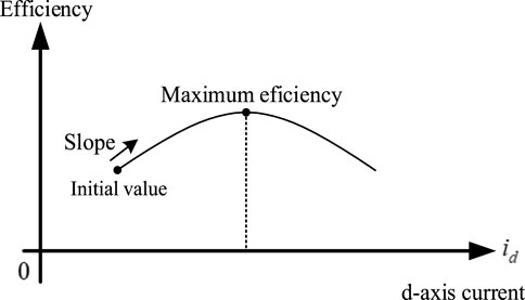
FIGURE 4. The concave curve of the efficiency to the d-axis current.

where $\eta$ is the efficiency, f is a quadratic function, and $q_1$ and b are the parameters of the quadratic function. By taking the differential of Eq. 16, one can obtain the following equation:

$i_d^{\ast }=\frac{b}{q_1}(17)$

where $i_d^{\ast }$ is the relative d-axis current, which provides the maximum efficiency of the IPMSM drive system. In the real world, however, IPMSMs require a step-by-step algorithm to search on-line for the maximum efficiency. In this paper, a steepest ascent method is used. The details are as follows:

First, the initial d-axis current is selected and expressed as $i_{d0}$. Then, the error between $i_d^{\ast }$ and $i_{d0}$ can be shown as follows:

$e\left(i_{d0}\right)=\frac{1}{2}(i_{d0}-i_d^{\ast })q_1(i_{d0}-i_d^{\ast })-b(i_{d0}-i_d^{\ast })(18)$

where $e\left(i_{d0}\right)$ is the error of the function f between the $i_{d0}$ and the $i_d^{\ast }$. Next, by taking the differential of Eq. 16, one can obtain that the gradient of the function f, which is expressed as follows:

$g\left(i_d\right)=\mathrm{\nabla }f\left(i_d\right)=q_1{i}_d-b(19)$

where $g\left(i_d\right)$ is the gradient at the $i_d$ current, and $\nabla f$ is the gradient of the function f.

After that, the d-axis current of the ${(k+1)}_{th}$ step can be described as the following equation:

${\left(i_d\right)}_{k+1}={\left(i_d\right)}_k+{\left({\alpha }_1\right)}_k{g}_k{\left(i_d\right)}_k(20)$

and then from Eq. 19, one can obtain the following equation:

$g_k{\left(i_d\right)}_k=q_1{\left(i_d\right)}_k-b(21)$

where ${\left(i_d\right)}_{k+1}$ is the d-axis current at the ${(k+1)}_{th}$ step, ${\left(i_d\right)}_k$ is the d-axis current at the ${\left(k\right)}_{th}$ step, and $g_k$ is the gradient of the function f at the ${\left(k\right)}_{th}$ step. Substituting Eqs. 20, 21 into Eq. 16, and then taking its partial differential to ${\left({\alpha }_1\right)}_k$, one can derive the following equation (Avriel, 1976):

$-{\mathrm{g}}_k{\left(i_d\right)}_k{q}_1{\left(i_d\right)}_k-q_1{\mathrm{g}}_k{\left(i_d\right)}_k{\left({\alpha }_1\right)}_k{g}_k{\left(i_d\right)}_k+g_k{\left(i_d\right)}_{k}b=0(22)$

From Eq. 22, one can obtain the following equation:

$\begin{array}{c}{\mathrm{g}}_k{\left(i_d\right)}_k(-q_1{\left(i_d\right)}_k+b)-q_1{\mathrm{g}}_k{\left(i_d\right)}_k{\left({\alpha }_1\right)}_k{g}_k{\left(i_d\right)}_k\\ ={\mathrm{g}}_k{\left(i_d\right)}_k{g}_k{\left(i_d\right)}_k-q_1{\mathrm{g}}_k{\left(i_d\right)}_k{\left({\alpha }_1\right)}_k{g}_k{\left(i_d\right)}_k=0\end{array}(23)$

From Eq. 23, it is not difficult to derive the step size, ${\left({\alpha }_1\right)}_k$, as the following equation:

${\left({\alpha }_1\right)}_k=\frac{g_k{\left(i_d\right)}_k{g}_k{\left(i_d\right)}_k}{q_1{g}_k{\left(i_d\right)}_k{g}_k{\left(i_d\right)}_k}=\frac{1}{q_1}(24)$

Finally, by substituting Eq. 24 into Eq. 20, one can obtain a simple equation for the ${\left(i_d\right)}_{k+1}$ as follows:

${\left(i_d\right)}_{k+1}={\left(i_d\right)}_k+\left(\frac{1}{q_1}\right)g_k{\left(i_d\right)}_k(25)$

3.2 Predictive speed-controller design

Predictive controllers have been developed and improved for 40 years. They can be used for single-input and single-output systems, multi-input and multi-output systems, with constraint and without constraint systems, and model-based and no model-based systems. Recently, due to the improvements in digital signal processors, predictive controller design has become very popular in power electronics and motor drives (Soeterboek, 1992). In this paper, a predictive controller is used for the speed-loop control for the IPMSM in this paper. The details are described as follows:

3.1.1 Predictive speed-controller without input constraint

The dynamic speed equation of an IPMSM without an external load is shown as follows:

$\frac{d}{dt}{\omega }_m=\frac{1}{J_t}(T_e-B_t{\omega }_m)=\frac{1}{J_t}(K_T{i}_q-B_t{\omega }_m)(26)$

where $K_T$ is the parameter of the torque constant. From Eq. 26, and converting the result into Laplace’s transformation, one can obtain the following equation:

$\begin{array}{l}{G}_p\left(s\right)=\frac{{\omega }_m\left(s\right)}{i_q\left(s\right)}\\ =\frac{K_T}{J_{t}s+B_t}\end{array}(27)$

Next, we can define the transfer function of the zero-order-hold device as follows:

$G_{zoh}\left(s\right)=\frac{1-e^{-s{T}_{sp}}}{s}(28)$

where $T_{sp}$ is the time interval of the zero-order-hold device. The approximation of the transfer function of the zero-order-hold device cascading with the IPMSM can be shown as follows:

$\begin{array}{l}{G}_{sp}\left(s\right)=G_{zoh}\left(s\right)G_p\left(s\right)\\ =\frac{1-e^{-s{T}_{sp}}}{s}\cdot \frac{K_T}{J_{t}s+B_t}\end{array}(29)$

Defining $e^{-s{T}_{sp}}=z^{-1}$ and then substituting it into Eq. 29, one can develop the following z-transformation equation:

$G_{sp}\left(z\right)=\frac{K_T}{B_t}(1-z^{-1})\left(\frac{z}{z-1}-\frac{z}{z-e^{-\frac{B_t}{J_t}{T}_{sp}}}\right)(30)$

From Eq. 30, it is not difficult to derive the following equation:

$G_{sp}\left(z\right)=\frac{{\omega }_m\left(z\right)}{i_q\left(z\right)}=\frac{K_T}{B_t}\left(\frac{1-e^{-\frac{B_t}{J_t}{T}_{sp}}}{z-e^{-\frac{B_t}{J_t}{T}_{sp}}}\right)(31)$

Taking the inverse z-transformation, one can obtain the following equation:

$\begin{array}{l}{\omega }_m(k+1)=e^{-\frac{B_t}{J_t}{T}_{sp}}{\omega }_m\left(k\right)+\frac{1-e^{-\frac{B_t}{J_t}{T}_{sp}}}{B_t}{K}_T{i}_q\left(k\right)\\ =a_s{\omega }_m\left(k\right)+b_s{i}_q\left(k\right)\end{array}(32)$

where $a_s$ is $e^{-\frac{B_t}{J_t}{T}_{sp}}$ and $b_s$ is $\frac{1-e^{-\frac{B_t}{J_t}{T}_{sp}}}{B_t}{K}_T$.

If we replace (k) with (k-1) and then use Eq. 32, we can derive the following equation:

${\omega }_m\left(k\right)=a_s{\omega }_m(k-1)+b_s{i}_q(k-1)(33)$

From Eqs. 32, 33, one can obtain the speed difference as the following equation:

$\mathrm{\Delta }{\omega }_m(k+1)=a_s\mathrm{\Delta }{\omega }_m\left(k\right)+b_s\mathrm{\Delta }{i}_q\left(k\right)(34)$

where $\mathrm{\Delta }{\omega }_m\left(k\right)$ is the speed difference at the $k_{th}$ sampling interval, $\mathrm{\Delta }{i}_q\left(k\right)$ is the q-axis current difference at the $k_{th}$ sampling interval. From Eqs. 33, 34, one can derive the estimated speed at the ($k+1$) sampling interval as the following equation:

$\begin{array}{l}{\widehat{\omega }}_m(k+1)={\omega }_m\left(k\right)+\mathrm{\Delta }{\omega }_m(k+1)\\ ={\omega }_m\left(k\right)+a_s\mathrm{\Delta }{\omega }_m\left(k\right)+b_s\mathrm{\Delta }{i}_q\left(k\right)\end{array}(35)$

It is possible to define the performance index $J_p\left(k\right)$, which includes the square of the speed error, and the square of the $\mathrm{\Delta }{i}_q\left(k\right)$ as the following equation:

$J_p\left(k\right)={\left[{\omega }_m^{\ast }(k+1)-{\widehat{\omega }}_m(k+1)\right]}^2+r_w{\left[i_q\left(k\right)-i_q(k-1)\right]}^2(36)$

where $r_w$ is the weighting factor. Submitting Eq. 35 into Eq. 36, one can obtain the following equations:

$\begin{array}{l}{J}_p\left(k\right)={\left[{\omega }_m^{\ast }(k+1)-{\omega }_m\left(k\right)-a_s\mathrm{\Delta }{\omega }_m\left(k\right)-b_s\mathrm{\Delta }{i}_q\left(k\right)\right]}^2\\ +r_w{\left[\mathrm{\Delta }{i}_q\left(k\right)\right]}^2\end{array}(37)$

and

$\mathrm{\Delta }{i}_q\left(k\right)=i_q\left(k\right)-i_q(k-1)(38)$

By rearranging Eq. 37, one can obtain the following equation:

$\begin{array}{l}{J}_p\left(k\right)=(b_s^2+r_w){\left[\mathrm{\Delta }{i}_q\left(k\right)\right]}^2-2b_s\left[{\omega }_m^{\ast }(k+1)-{\omega }_m\left(k\right)-a_s\mathrm{\Delta }{\omega }_m\left(k\right)\right]\mathrm{\Delta }{i}_q\left(k\right)\\ +\left[{\omega }_m^{\ast }(k+1)-{\omega }_m\left(k\right)-a_s\mathrm{\Delta }{\omega }_m\left(k\right)\right]\end{array}(39)$

By taking the differential of $J_p\left(k\right)$ and $\mathrm{\Delta }{i}_q\left(k\right)$, and then assuming the result to be zero, one can develop the following equation:

$2(b_s^2+r_w)\mathrm{\Delta }{i}_q\left(k\right)-2b_s\left[{\omega }_m^{\ast }(k+1)-{\omega }_m\left(k\right)-a_s\mathrm{\Delta }{\omega }_m\left(k\right)\right]=\text{ 0}(40)$

From Eq. 40, the desired q-axis current difference command can be expressed as follows:

$\mathrm{\Delta }{i}_q^{\ast }\left(k\right)=\frac{b_s\left({\omega }_m^{\ast }(k+1)-{\omega }_m\left(k\right)\right)}{b_s^2+r_w}-\frac{a_s{b}_s\mathrm{\Delta }{\omega }_m\left(k\right)}{b_s^2+r_w}(41)$

Finally, the q-axis current command can be obtained as follows:

$i_q^{\ast }\left(k\right)=i_q(k-1)+\mathrm{\Delta }{i}_q^{\ast }\left(k\right)(42)$

3.1.2 Predictive speed-controller with input constraint

It is possible to rewrite the constraints as the following two equations:

$i_q\left(k\right)\le i_q^{max}(43)$

and

$-i_q\left(k\right)\le -i_q^{min}(44)$

However, in this paper, we focus on the q-axis current difference. As a result, Eqs. 43, 44 can be expressed as the following two equations:

$i_q(k-1)+\mathrm{\Delta }{i}_q\left(k\right)\le i_q^{max}(45)$

and

$-i_q(k-1)-\mathrm{\Delta }{i}_q\left(k\right)\le -i_q^{min}(46)$

By combing Eqs. 45, 46, one can obtain the following three equations (Wang, 2009):

$\mathrm{\nabla }\text{U}\left(k\right)=M\mathrm{\Delta }{i}_q\left(k\right)\le \gamma (47)$

$M=\left[\begin{array}{c}1\\ -1\end{array}\right](48)$

and

$\gamma =\left[\begin{array}{c}{i}_q^{max}-i_q(k-1)\\ -i_q^{min}+i_q(k-1)\end{array}\right](49)$

A Lagrange multiplier is used in this paper to combine the constraint and the performance index. Then the following equation can be obtained:

$\begin{array}{l}\mathrm{\nabla }{J}_p\left(k\right)={\lambda }_{lagr}^T\mathrm{\nabla }\text{U}\left(k\right)\\ ={\left[\begin{array}{c}{\lambda }_{max}\\ {\lambda }_{min}\end{array}\right]}^T\mathrm{\nabla }\text{U}\left(k\right)\end{array}(50)$

where ${\lambda }_{max}$ is the multiplier of the maximum q-axis current, and ${\lambda }_{min}$ is the multiplier of the minimum q-axis current.

By combining the constraint and the performance $J_p\left(k\right)$, one can define a new performance index $J_{lagr}\left(k\right)$. Then the $J_{lagr}\left(k\right)$ can be defined as the following equation:

$J_{lagr}\left(k\right)=J_p\left(k\right)+{\lambda }_{lagr}^T\mathrm{\nabla }\text{U}\left(k\right)(51)$

Submitting Eqs. 39, 47 into Eq. 51, one can derive the $J_{lagr}\left(k\right)$ as the following equation:

$\begin{array}{l}{J}_{lagr}\left(k\right)=(b_s^2+r_w){\left[\mathrm{\Delta }{i}_q\left(k\right)\right]}^2-2b_s\left[{\omega }_m^{\ast }(k+1)-{\omega }_m\left(k\right)-a_s\mathrm{\Delta }{\omega }_m\left(k\right)\right]\mathrm{\Delta }{i}_q\left(k\right)\\ +\left[{\omega }_m^{\ast }(k+1)-{\omega }_m\left(k\right)-a_s\mathrm{\Delta }{\omega }_m\left(k\right)\right]+{\lambda }_{lagr}^T(M\mathrm{\Delta }{i}_q\left(k\right)-\gamma )\end{array}(52)$

Then by using the differential of $J_{lagr}\left(k\right)$ to $\mathrm{\Delta }{i}_q\left(k\right)$ and assuming its result to be zero, one can obtain the following equation:

$2(b_s^2+r_w)\mathrm{\Delta }{i}_q\left(k\right)-2b_s\left[{\omega }_m^{\ast }(k+1)-{\omega }_m\left(k\right)-a_s\mathrm{\Delta }{\omega }_m\left(k\right)\right]+M^T{\lambda }_{lagr}=\text{ 0}(53)$

Rearranging Eq. 53, one can obtain the following equation:

$\mathrm{\Delta }{i}_q\left(k\right)=\mathrm{\Delta }{i}_q^{\ast }\left(k\right)-\frac{M^T{\lambda }_{lagr}}{b_s^2+r_w}(54)$

where $\mathrm{\Delta }{i}_q^{\ast }\left(k\right)$ is the q-axis current difference without a constraint. After that, the multiplier ${\lambda }_{lagr}$ needs to be derived. The details are discussed as follows. First, in Eq. 52, by using the differential of $J_{lagr}\left(k\right)$ to ${\lambda }_{lagr}$ and assuming its result to be zero, one can obtain the following equation (Wang et al., 2015):

$M\mathrm{\Delta }{i}_q\left(k\right)-\gamma =\text{ 0}(55)$

Next, from Eq. 54, one can obtain the following equation:

$M\mathrm{\Delta }{i}_q\left(k\right)=M\mathrm{\Delta }{i}_q^{\ast }\left(k\right)-\frac{M{M}^{\text{T}}{\text{λ}}_{\text{lagr}}}{b_s^2+r_w}(56)$

Submitting Eq. 56 into Eq. 55, one can derive the following equation:

$M\mathrm{\Delta }{i}_q^{\ast }\left(k\right)-\frac{M{M}^{\text{T}}{\text{λ}}_{\text{lagr}}}{b_s^2+r_w}-\gamma =0(57)$

Finally, the Lagrange multiplier is shown as follows:

${\text{λ}}_{\text{lagr}}=\left(b_s^2+r_w\right)\left(\left[\begin{array}{c}1\\ -1\end{array}\right]\mathrm{\Delta }{i}_q^{\ast }\left(k\right)-\left[\begin{array}{c}{i}_q^{max}-i_q(k-1)\\ -i_q^{min}+i_q(k-1)\end{array}\right]\right)=\left[\begin{array}{c}{\lambda }_{\mathit{max}}\\ {\lambda }_{\mathit{min}}\end{array}\right](58)$

In the real world, the ${\lambda }_{lagr}$ must be equal to or larger than zero. To meet this requirement, Hildreth’s quadratic programming procedure is used here (Wang et al., 2015). By using an iterative method, the optimal multiplier ${\lambda }_{lagr}$, is expressed as follows:

${\lambda }_{lagr}=\left[\begin{array}{c}{\lambda }_{max}^{\ast }\\ {\lambda }_{min}^{\ast }\end{array}\right](59)$

Submitting Eq. 59 into Eq. 54, one can obtain the following equation:

$\begin{array}{l}\mathrm{\Delta }{i}_{q\_new}^{\ast }\left(k\right)=\mathrm{\Delta }{i}_q^{\ast }\left(k\right)-\frac{M^T{\lambda }_{lagr}}{b_s^2+r_w}\\ =\mathrm{\Delta }{i}_q^{\ast }\left(k\right)-\frac{{\lambda }_{max}^{\ast }-{\lambda }_{min}^{\ast }}{b_s^2+r_w}\end{array}(60)$

Finally, the q-axis current command, which considers the input constraint, can be expressed as follows:

$i_{q\text{\_}new}^{\text{*}}\left(k\right)=i_q(k-1)+\Delta i_{q\_new}^{\ast }\left(k\right)(61)$

In order to explain in a more detailed way, Figure 5A shows the block diagram of the proposed predictive controller with an input constraint. The control algorithm includes an input constraint, a predictive control parameter without considering constraints, an uncontrolled plant, and an integration. First, the speed command ${\omega }_m^{\ast }(k+1)$ is compared to the feedback speed ${\omega }_m\left(k\right).$ Then, the speed error is multiplied by the constant gain $b_s$. In addition, the speed difference, $\mathrm{\Delta }{\omega }_m\left(k\right)$ is multiplied by the constant gain $a_s{b}_s$. Next, the difference between these two results is multiplied by $\frac{1}{b_s^2+{\gamma }_w}$ to obtain $\mathrm{\Delta }{i}_q^{\ast }\left(k\right)$. After that, the, $i_q^{\min }$, $i_q^{\max }$, and $i_q(k-1)$ are used to compute $\mathrm{\Delta }{i}_{q\_new}^{\ast }\left(k\right)$. Finally, $i_{q\text{\_}new}^{\text{*}}\left(k\right)$, which is the q-axis command with a constraint, is obtained and sent out to the IPMSM drive system. Then a closed-loop drive system is thus achieved.

FIGURE 5

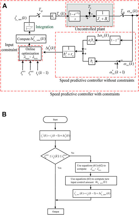
FIGURE 5. Predictive controller with input constraint. (A) Block diagram (B) flow chart.

Figure 5B shows the flow-chart of the predictive controller with an input constraint. First, the q-axis current command $i_q^{\text{*}}\left(k\right)$ is computed. Next, the $i_q^{\text{*}}\left(k\right)$ is checked to determine if it is between $i_q^{\min }$ and $i_q^{\max }$. If it is, then the $i_q^{\text{*}}\left(k\right)$ is sent out to control the IPMSM drive system. Otherwise, the ${\lambda }_{max}^{\ast }$ and the ${\lambda }_{min}^{\ast }$ are used to determine the $\mathrm{\Delta }{i}_{q\_new}^{\ast }\left(k\right)$, which is the q-axis current difference with a constraint. Finally, the ${}_{q\text{\_}new}{}^{\ast }\left(k\right)$, which is the q-axis current command with a constraint, is sent out to control the IPMSM drive system.

4 Experimental results

The experimental results include two parts: background of Experimental Setting and measured results.

4.1 Background of experimental setting

The block diagram of the implemented IPMSM drive system is shown in Figure 6A, which includes a predictive speed controller, a PI current controller, a d-q axis to a-b-c axis coordinate transformation, a SVPWM modulator, an a-b-c axis to d-q axis coordinate transformation, an A/D converter, an inverter, and an IPMSM. The sampling interval of the speed-loop control is 1 ms, and the sampling interval of the current-loop control is 100 $\mu s$. First, the speed command ${\omega }_m^{\ast }$ is compared to the feedback speed ${\omega }_m$. Then the speed error is processed by the predictive speed-controller to generate the q-axis current command $i_q^{\ast }$. The d-axis current command $i_d^{\ast }$ is determined by the calculated efficiency $\eta$ and the steepest ascent tracking method. The efficiency $\eta$ uses the torque $T_e$ multiplied by the mechanical speed ${\omega }_m$ and then is divided by input power $P_{in}$, which is the DC-link voltage $V_{dc}$ multiplied by the DC-link current $I_{dc}$. After that, the d-q axis current commands are compared to the feedback d-q axis currents $i_d$ and $i_q$. Next, the PI current controller is used to generate the d-q axis voltage commands $v_d^{\ast }$ and $v_q^{\ast }$. A d-q axis to a-b-c axis coordinate transformation is then used to convert $v_d^{\ast }$ and $v_q^{\ast }$ into the a-b-c axis voltage commands $v_a^{\ast }$, $v_b^{\ast }$, and $v_c^{\ast }$. After that, a SVPWM modulator is used to generate the six gating signals of the inverter. Finally, the IPMSM is rotated and a closed-loop IPMSM dive system is thus achieved.

FIGURE 6

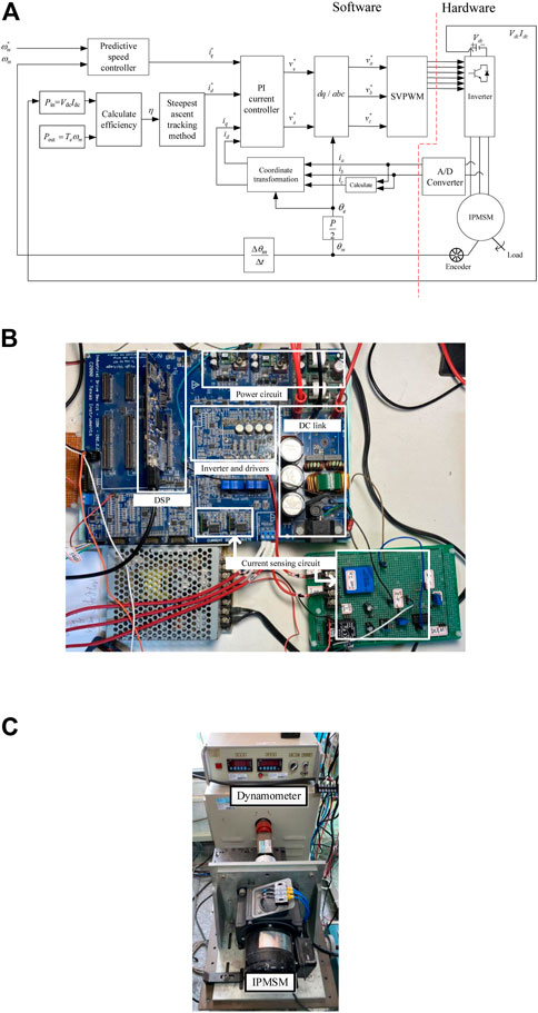
FIGURE 6. Implemented IPMSM drive system. (A) Block diagram (B) hardware circuit (C) dynamometer.

Figure 6B shows a photograph of the hardware circuit, which includes a digital signal processor (DSP), an inverter and its driver, a power circuit which includes six IGBTs, a DC-link capacitor and a small inductor, and a current sensing circuit. Figure 6C shows a photograph of the IPMSM connected to a dynamometer, which is used for the adding an external load test.

4.2 Measured results

Several experimental results are shown in this paper to validate the theoretical analysis. Figure 7A shows the measured efficiency tracking response when using a 0.1A fixed step-size d-axis current. As can be observed, the IPMSM drive system requires 14 steps to reach its maximum efficiency, which is near 85%. Figure 7B shows the measured efficiency tracking response by using the steepest ascent method. This IPMSM drive system only takes four steps to reach its maximum efficiency. In addition, the step-size is gradually reduced as the IPMSM drive system approaches its maximum efficiency point. Figure 8A shows the relationship between the efficiency and motor speeds. As can be observed, the variations of the efficiency are quite small when the motor is operated from 600 r/min to 2000 r/min. Figure 8B show the relationship between the efficiency to the d-axis current, which is varied between 0 and 1A. The results shown in Figure 8B are very close to a concave curve. As a result, there is only one maximum efficiency point, which is also the global maximum point as well. It is feasible to use the steepest ascent method to search for the maximum point for a concave curve. From Figures 8A,B, we can see that the measured efficiency and the calculated efficiency are quite similiar.

FIGURE 7

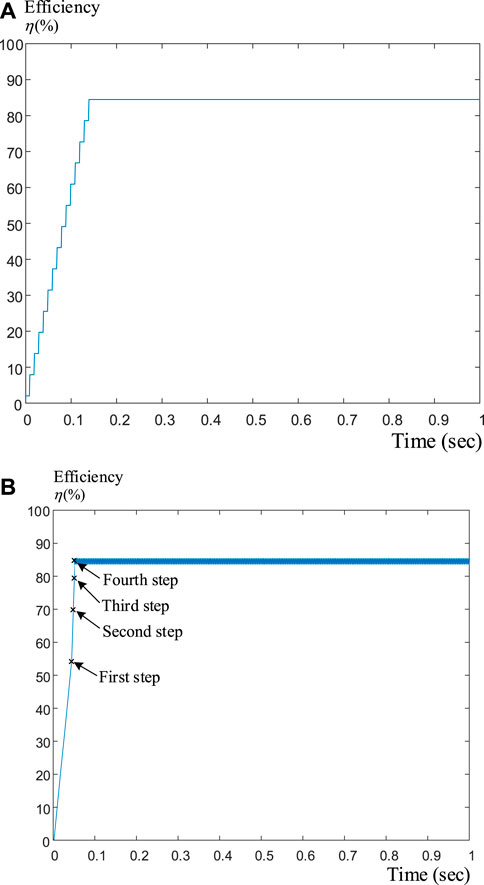
FIGURE 7. Maximum efficiency tracking responses at 600 r/min with a 3 Nt. m load. (A) Using 0.1A fixed-step d-axis current (B) using steepest ascent method.

FIGURE 8

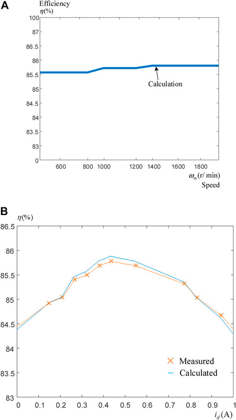
FIGURE 8. The relationship between efficiency and speed and efficiency and d-axis current. (A) Efficiency and speeds (B) efficiency and the d-axis current at 600 r/min and 3 N m load.

Figure 9A demonstrates the input line-voltage of the IPMSM, $v_{ab}$, which has a 10 kHz PWM switching frequency. By using the space-vector PWM modulation method, from $0°$ to $180°$, the voltage $v_{ab}$ is positive, and from $180°$ to $360°$, the voltage $v_{ab}$ is negative. In addition, the amplitude of the $v_{ab}$ is near 250V. Figure 9B shows the input a-phase current of the IPMSM. The a-phase current has a near sinusoidal waveform with low current ripples.

FIGURE 9

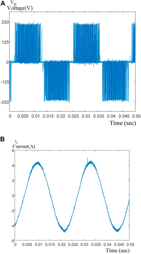
FIGURE 9. Measured input voltage and current of the IPMSM. (A) Input voltage (B) input current.

Figure 10A displays the comparison of the speed responses by using a PI speed-loop controller and the predictive speed-loop controller. The parameters of the PI controller are determined by using a pole-assignment technique that has the same rise time as the predictive controller. As can be observed, the predictive controller has a lower overshoot and a shorter time to reach steady-state conditions. Figure 10B shows the relative q-axis current responses. The predictive controller provides a smaller peak current and greater input power than the PI controller. Figure 11A demonstrates the comparison of the predictive controller with and without a constraint. The predictive controller with a constraint has a lower overshoot than the predictive controller without a constraint. Figure 11B demonstrates the relative q-axis current. The predictive controller with a constraint has a smaller peak current, greater input power, and fewer ringing currents than the predictive controller without a constraint.

FIGURE 10

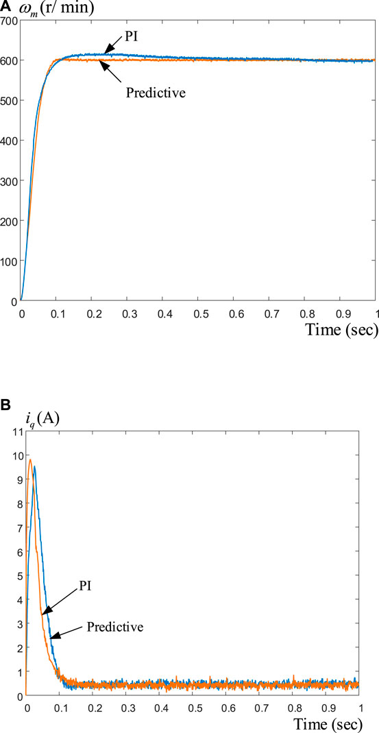
FIGURE 10. Measured transient responses at 600 r/min using predictive controller and PI controller. (A) Speed responses (B) q-axis current responses.

FIGURE 11

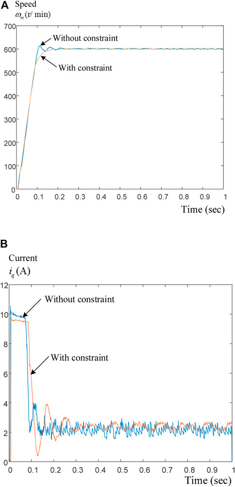
FIGURE 11. Measured transient responses at 600 r/min using predictive controller with and without constraints (A) speed responses (B) q-axis current responses.

Figure 12A shows the comparison of the speed responses when an external load of 3 N m is added at 600 r/min. The predictive controller has a 10 r/min speed drop and a 0.2 s recovery time. The PI controller, however, has a 40 r/min speed drop and a 0.35 s recovery time. Figure 12B demonstrates the relative q-axis current responses. The PI controller provides more ringing currents than the predictive controller. Figure 13 shows the measured responses at different speed commands from 10 r/min to 1800 r/min. All of the responses are very quick and linear. These results can demonstrate that the predictive speed-loop controller can provide better performance than the PI controller.

FIGURE 12

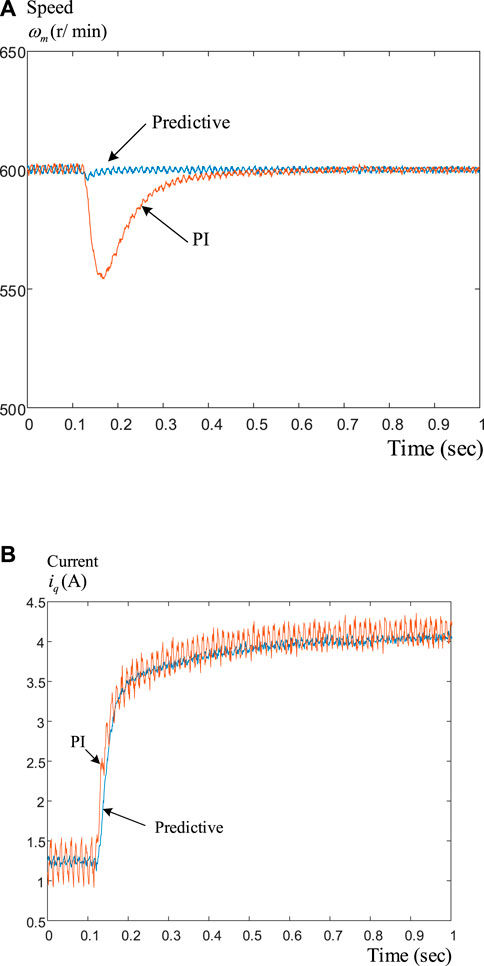
FIGURE 12. Measured load disturbance responses at 600 r/min. (B) Speed responses (B) q-axis current responses.

FIGURE 13

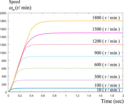
FIGURE 13. Measured responses at different speed commands.

5 Conclusion

In this paper, a maximum efficiency IPMSM control system with a predictive-speed controller design is investigated. By using the steepest ascent method, the searching times to reach the maximum efficiency can be effective reduced to 4 steps; however, by using the traditional fixed step method, the searching times to reach the maximum efficiency requires 14 steps. In addition, by using a predictive speed-controller, the transient response of the predictive controller is faster with a 2% reduction of overshoot than the PI controller. In addition, the predictive speed-control IPMSM drive system has a smaller speed drop, which is only near 10% of the PI controller, and quicker recovery time, which is only 25% of the PI speed-control. The proposed predictive-speed control IPMSM drive system can be operated from 10 r/min to 1800 r/min with satisfactory linear responses. The proposed method can be easily and effectively applied in motor drives for air conditioners, vacuum cleaners, and lawn movers.

Data availability statement

The original contributions presented in the study are included in the article/Supplementary Material, further inquiries can be directed to the corresponding author.

Author contributions

T-HL: English paper preparation, funding, advise. Y-HZ: Hardware design, DSP program coding, integration, testing, experimental waveform collections.

Funding

The paper is supported by Ministry of Science and Technology, under Grant MOST 110–2221-E-011–086.

Conflict of interest

The authors declare that the research was conducted in the absence of any commercial or financial relationships that could be construed as a potential conflict of interest.

Publisher’s note

All claims expressed in this article are solely those of the authors and do not necessarily represent those of their affiliated organizations, or those of the publisher, the editors and the reviewers. Any product that may be evaluated in this article, or claim that may be made by its manufacturer, is not guaranteed or endorsed by the publisher.

References

Avriel, M. (1976). Nonlinear programming analysis and methods. New Jersey: USA: Prentice-Hall.

Google Scholar

Balamurali, A., Feng, G., Kundu, A., Dhulipati, H., and Kar, N. C. (2020). Noninvasive and improved torque and efficiency calculation toward current advance angle determination for maximum efficiency control of PMSM. IEEE Trans. Transp. Electrific. 6 (1), 28–40. doi:10.1109/tte.2019.2962333

CrossRef Full Text | Google Scholar

Balamurali, A., Kundu, A., Li, Z., and Kar, N. C. (2021). Improved harmonic iron loss and stator current vector determination for maximum efficiency control of PMSM in EV applications. IEEE Trans. Ind. Appl. 57 (1), 363–373. doi:10.1109/tia.2020.3034888

CrossRef Full Text | Google Scholar

Bose, B. K. (2002). Modern power electronics and AC drives. New Jersey, USA: Prentice-Hall.

Google Scholar

Caruso, M., Tommaso, A. O. D., Genduso, F., and Miceli, R. (2014). “Experimental investigation on high efficiency real-time control algorithms for IPMSMs,” in 2014 International Conference on Renewable Energy Research and Application (ICRERA) (Milwaukee, WI, USA: IEEE), 974–979. doi:10.1109/ICRERA.2014.7016531

CrossRef Full Text | Google Scholar

Ding, X., Liu, G., Du, M., Guo, H., Duan, C., and Qian, H. (2016). Efficiency improvement of overall PMSM-inverter system based on artificial bee Colony algorithm under full power range. IEEE Trans. Magn. 52 (7), 11–14. doi:10.1109/tmag.2016.2526614

CrossRef Full Text | Google Scholar

Kooning, J. D. M., Vyver, J. V., Meersman, B., and Vandevelde, L. (2017). Maximum efficiency current waveforms for a PMSM including iron losses and armature reaction. IEEE Trans. Ind. Appl. 53 (4), 3336–3344. doi:10.1109/tia.2017.2681619

CrossRef Full Text | Google Scholar

Liu, T., and Fadel, M. (2018). An efficiency-optimal control method for mono-inverter dual-PMSM systems. IEEE Trans. Ind. Appl. 54 (2), 1737–1745. doi:10.1109/tia.2017.2768535

CrossRef Full Text | Google Scholar

Mahmud, M. H., Wu, Y., and Zhao, Y. (2020). Extremum seeking-based optimum reference flux searching for direct torque control of interior permanent magnet synchronous motors. IEEE Trans. Transp. Electrific. 6 (1), 41–51. doi:10.1109/tte.2019.2962327

CrossRef Full Text | Google Scholar

Soeterboek, R. (1992). Predictive control-A unified approach. New Jersey, USA: Prentice-Hall.

Google Scholar

Takaashi, A., and Oguro, R. (2009). “A method of high efficiency control for IPMSM by disturbance observer,” in 2009 International Conference on Power Electronics and Drive Systems (PEDS), 637–642. doi:10.1109/PEDS.2009.5385899

CrossRef Full Text | Google Scholar

Wang, L., Chai, S., Yoo, D., Gan, L., and Ng, K. (2015). PID and predictive control of electrical drives and power converters using MATLAB/simulink. Singapore: Wiley & Sons.

Google Scholar

Wang, L. (2009). Model predictive control system design and implementation using MATLAB. London, UK: Springer.

Google Scholar

Yang, S., Liu, K., Hu, Y., Chu, L. L., and Chen, S. (2018). “Efficiency optimization control of IPMSM considering varying machine parameters,” in 2018 IEEE Student Conference on Electric Machines and Systems (Huzhou, China: IEEE). doi:10.1109/SCEMS.2018.8624761

CrossRef Full Text | Google Scholar