A Procedural Method to Predictively Assess Power-Quality Trade-Offs of Circuit-Level Adaptivity in IoT Systems

1 Introduction

Over the last decade, we have witnessed the explosion of Internet-of-Things (IoT) applications and devices. With 11.7 billion connected IoT devices at the end of 2020, it is expected that this number will keep growing to about 30 billion in 2025 IOT Analytics (2020). This has surged the demand for devices that show both improved functionality and better energy efficiency, to enhance their embedded nature and increase their sustainability. At the core of these IoT devices are integrated circuits (ICs), enabling the sensor node to sense, process information, and communicate with other nodes in the network Alioto (2018). Improving the overall energy efficiency of IoT devices is, thus, directly related to an increase in the energy efficiency of ICs. In that regard, since the formalization of Moore’s law, the main contributor to the reduction of energy consumption in ICs has been the advancement of IC technology, enabling to a large extent the 100 × energy reduction per decade we observed Alioto (2017). However, drastic improvements in energy efficiency cannot rely on technological advancements anymore, as it is estimated that they will contribute to reducing energy only by 4 × in the next decade Alioto (2017). Novel design approaches are required to continue the energy reduction for the next generation of IoT nodes.

A popular methodology to increase the node’s energy efficiency and increase battery life is known as context-aware adaptivity Chatterjee et al. (2019). We define adaptivity as the ability to change the way of operating the sensor node based on the perceived context, i.e., based on external or internal changes over time. An external change (also called environmental change) is, for example, the increase of background noise of speech recognition sensor nodes, requiring a higher-effort operating mode in the sensor node. An internal change is, for example, a low battery supply, preferring a lower-effort operation mode in the sensor node. Context-aware adaptation has been successfully developed for digital systems, such as processors, sensor nodes, or wireless communication nodes Meghdadi and Bakhtiar (2014), Sen et al. (2014), Cao et al. (2017), Fallahzadeh et al. (2017), Chatterjee et al. (2020), Maroudas et al. (2021). Moreover, ICs are subjected to increasing design constraints. More advanced fabrication technologies increase the susceptibility of ICs to numerous variations (manufacturing, aging, etc.), increasing the design margin for resiliency. As a result, complex design trade-offs are necessary to obtain an optimal design, calling for the use of automated and generic methodologies.

In that regard, a critical challenge is precisely the large variety of methods applied, which are typically bound to a given circuit and target application. A more generic approach has been conceptualized as energy-quality (EQ) scalability, where quality represents how well a certain task is performed Alioto et al. (2018). Commercial ICs are typically based on a “worst-case” design, which implies that margins are taken such that the circuit would work in the worst conditions; i.e., it is designed for a (fixed) maximum quality. In practice, this worst case will almost never be encountered; hence, the quality demanded by the application will be almost constantly lower than this maximum. Essentially, the EQ scalability can then make use of a given quality slack, which represents the difference as illustrated in Figure 1A. It includes margins according to the application or task, the current usage (the same application may require several quality levels), or the dataset (different inputs of the same application and context may require different quality levels), which can be traded off against energy in context-aware adaptivity. EQ scalability methods have already been applied to numerous designs, e.g., sensor nodes (Badami et al., 2015; Cao et al., 2017; Ieong et al., 2017; Xin et al., 2018; De Roose et al., 2020), digital circuits, (Moons and Verhelst, 2014; Rizzo, 2019), and edge Artificial Intelligence (AI) hardware Peluso and Calimera (2019). It has also been identified among key factors to enable the next-generation IoT nodes and communications nodes for 5G and 6G Mahmood et al. (2020); Shafique et al. (2020).

FIGURE 1

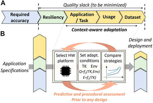
FIGURE 1. (A) The concept of quality slack, adapted from the work of Alioto (2017), and (B) overview of the proposed methodology.

Yet, one remaining issue is that with most adaptive strategies, it is not possible to easily assess if and how much gain, resp. overhead they would lead to in the final system before implementing it. The quality is measured differently for each system and application, and the optimal settings are issued from complex relationships between the different performances to be adapted and the tuning settings. Assessing the effectiveness of a proposed adaptation methodology prior to any design would enable system designers to benchmark potential adaptive strategies and their gains/overhead in various scenarios or evaluate the reuse of the hardware platforms for several applications. Moreover, it allows the designers to make an educated choice on what strategy to choose, before investing in the strategy.

To solve this issue, we propose to take a step back and analyze adaptivity from a more theoretical point of view. In particular, our objective is to develop an adaptation methodology that is at the same time generic and predictive; i.e., the results can be generated prior to any design of the associated circuitry, as shown in Figure 1B. Taking foundations in the EQ scalability concept, we will study adaptivity in several ways, constituting the main contributions of this work:

• Analyzing the costs and benefits of generic adaptivity in energy-limited sensor nodes, first from a general design and manufacture point of view and then zooming into technical specifications such as power and quality scalability

• Creating a methodology to quickly estimate the potential power savings by enabling adaptivity prior to hardware development and comparing it to the added power consumption cost of adaptivity

• Applying these principles first to a theoretical use case, followed by three SotA-adaptive IoT systems taken from the literature Cao et al. (2017); Ieong et al. (2017); De Roose et al. (n d), to show its potential

This article is structured as follows: Section 2 starts with discussing the state of the art, followed by Section 3, which analyzes the high-level costs and benefits of adaptivity. Next, in Section 4, we use mathematics to estimate benefits stemming from adaptivity. Finally, in Section 5, the proposed methodology is deployed on three adaptivity studies from the SotA, where we benchmark our outcomes against the reported results of these works.

2 Taxonomy of Adaptive Circuits and State of the Art

The term adaptive is a broad term that comes with various connotations in the literature on low-power electronic systems. Surveys have been conducted on various viewpoints of adaptivity, e.g., the work of Chatterjee et al. (2019) about context-aware IoT systems, the work of Eldash et al. (2017) about on-chip intelligence, the work of Rizzo (2019) about adaptive design methodologies for digital ICs, and the work of Alioto et al. (2018) on energy-quality scalable systems. This diverging landscape is rooted in the fact that the adaptation strategy can be conducted for several physical layers—from network protocols to hardware implementations—and at different development phases—before, during, and/or after deployment. In this section, we attempt to present a taxonomy of adaptivity methods in micro-electronics, extending the work of Andraud and Verhelst (2018), with a focus on circuit-level adaptivity. This taxonomy will be illustrated with representative works from the related literature.

2.1 Proposed Taxonomy of Adaptive Circuits

Essentially, we discriminate between two crucial factors when designing an adaptive circuit: 1) the adaptation strategy, i.e., what part of the quality stack is targeted and how, and 2) the adaptation level, i.e., defining the amount of decision taken on the chip.

2.1.1 Adaptation Strategy

In the paradigm of the previously explained EQ scalability concept, plenty of design solutions have been presented, often named as context-aware adaptation or hierarchical systems. First, any adaptation strategy must consider which part of the quality slack will be tackled. The quality slack contains not only design resiliency (margins for process, voltage, or temperature variations) and margins for operating in several contexts (the wireless link quality, etc.) but also the task at hand and current system workload. Based on this observation, we can build EQ-scalable systems, which intend to consume (part of) the quality slack under current quality requirements to minimize energy, or conversely maximize the quality under a given energy constraint. Second, we can set the adaptation strategy. Typically, EQ scalability can be seen by dividing the possible operating conditions into a set of environments, measuring the current environment through sensors, evaluating the quality slack in this environment, and optimizing the operation of the circuit accordingly. To realize this, a large number of techniques have been presented for IoT nodes Cao et al. (2017); Teo et al. (2020), processors Gligor et al. (2009); Moons and Verhelst (2014), health monitoring Anzanpour et al. (2017); Ieong et al. (2017), sensor interfaces Trakimas and Sonkusale (2011); Badami et al. (2015); Teerapittayanon et al. (2016); Fallahzadeh et al. (2017); Giraldo et al. (2019); De Roose et al. (2020), or wireless transceivers Banerjee et al. (2017).

2.1.2 Adaptation Level

The amount of decisions that are taken on chip (i.e., where does adaptation happen) is the other crucial criterion to consider when designing an adaptive circuit. This adaptation level is important, as it is directly linked to the number of resources necessary to perform the adaptation. We will distinguish four general categories along this axis, ordered by a growing amount of on-chip resources.

2.1.2.1 Fixed

System settings are not tunable. In this case, settings are fixed at design time and never change so that no decision is taken on chip. An example of such a design is given in the study by Chen et al. (2012). We can refer to this as level zero.

2.1.2.2 Offline Configurable (OfC)

In OfC designs, as illustrated in Figure 2, system settings are tunable, but all are pre-defined before run time. During operation, the system does not switch between settings. This brings the benefit of efficiently using a single flexible hardware platform across multiple applications. An example of OfC designs is given in the study by Huang et al. (2014), where several sensors are integrated into a configurable biomedical platform and sensing front end. The user can select the sensors that are activated and configure a unique interface to measure each sensor. Other sensors could be also integrated into this platform using the same interface, hence reducing the design cost and time.

FIGURE 2

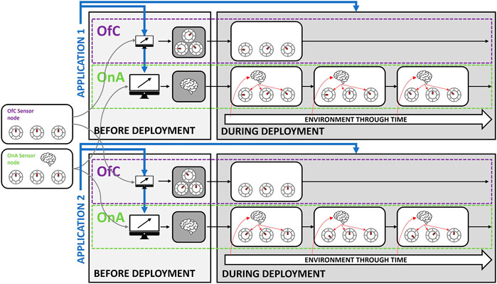
FIGURE 2. The difference between offline configurability and online adaptivity: a flexible platform is used for both OnA and OfC. Before deployment, static settings are configured for OfC, while an adaptive strategy is programmed onto the flexible platforms for OnA. During employment, the settings of OnA can, hence, change, based on a changing environment.

2.1.2.3 Online Adaptivity (OnA)

In OnA designs, as shown in Figure 2, the system is run time tunable, with a programmed adaptation strategy that is optimized offline, before run time. For instance, De Roose et al. (2020) in their study used offline optimization based on evolutionary algorithms that automatically derive optimal behavioral trees, which are then executed online. These behavioral trees contain the conditions necessary to migrate the circuit to a given mode and the associated optimal settings corresponding to this mode. Fallahzadeh et al. (2017) in their study used an adaptive compressed sensing scheme in the context of activity recognition. Here, the compression settings are changed for each activity using pre-optimized settings stored in a look-up table. OnA designs have also been applied to radio frequency transceivers, for instance, in the studies by Sen et al. (2012) and Meghdadi and Bakhtiar (2014). The general principle is to derive the optimal settings of some circuit-tuning parameters to achieve the best trade-off between power and performance over multiple channel conditions. These settings can be biased or power supply voltages of the main circuit blocks, different communication protocols, or digital control blocks. Process variations can also be integrated into the loop (Sen et al., 2014) to compensate for a greater part of the quality slack.

2.1.2.4 Online Learned

The system is tunable and able to figure out the best adaptation strategy fully on chip at run time; i.e., no pre-computation of parameters are necessary. The range of illustrative techniques is very large, from compensating one specific variation (one time), compensating for variations when the system is not in use (on-idle times), or continuously monitoring and optimizing the circuit while running (self-learning). One-time OnL has been demonstrated in, e.g., self-calibration circuits, such as in the work of Lee et al. (2018), which measure and calibrate their performances against process variations on chip. On the other end of the spectrum sits the self-learning transceiver developed by Banerjee et al. (2017), where the objective is to learn, in an unsupervised way, the optimal power versus performance trade-off according to multiple channel conditions. The current operating condition is either associated with a given cluster with available optimal settings, or the system is trained for this new condition using embedded machine learning, forming a new cluster. This strategy could, for instance, run in an embedded processor. While OnA optimizes only before deployment, OnL can further optimize at run time, adapting better to knowledge and data trends that are gathered after the start of the deployment.

3 Adaptivity: Costs and Benefits

According to the previous taxonomy, this work will focus on EQ systems adapted during run time and will compare and optimize the possibilities offered by OnA and OfC, assuming theoretical complete knowledge of the application. OnL can be seen as an extension to OnA that is closer to this theoretical complete knowledge. The costs of OnL, however, will not be discussed further in this article, as its strategies are typically very diverse and application dependent, while we intend to propose a unique methodology and optimization framework applicable to virtually any IoT application. Before entering into the details of the proposed mathematical framework, we will review the requirements, advantages, and disadvantages of adaptivity in this section.

3.1 Adaptivity Requirements

Adaptivity relies on three main functionalities, flexibility, awareness, and control, as depicted in Figure 3. We define these parameters as follows:

• Flexibility is the ability of a node to change its settings, here denoted as tuning knobs (TKs), which have an impact on both the quality and power consumption of the system. An example of flexibility is changing the sampling frequency in an IoT sensor node.

• Awareness is the ability to detect changes in the environment and/or its own state. An environmental state is defined as a set of transient sensor data characteristics that are correlated with the difficulty of the sensory task. For example, in a speech recognition application, environments differ in terms of signal-to-noise ratio (SNR).

• Control is the programmable brain of adaptivity. It links all environments and/or internal states to their respective optimal TK settings, for example, the decision to slow down instead of maintaining or speeding up processor clock frequency when a temperature sensor detects overheating.

FIGURE 3

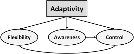
FIGURE 3. Building blocks of adaptivity.

3.2 Benefits of Adaptivity

The benefits of adaptivity can be assessed for both the simpler OfC and the complete OnA approach.

3.2.1 Offline Configurability Benefits

OfC enables reusing a flexible hardware platform across many applications if designed generally enough Huang et al. (2014). Hence, the design costs of such a platform can be split over multiple projects. Furthermore, the production cost of micro-electronics decreases per chip when the production volume increases. A single platform used across multiple applications allows for higher volumes, reducing production costs per unit. Second, flexible hardware platforms steeply reduce the time-to-market for an application, as the design of an ASIC (application-specific integrated circuit) usually takes months or years. Third, the risk of attempting to find new applications using the same hardware platform steeply decreases, as the design of a new hardware platform is usually the main contributing cost in these cases.

3.2.2 Added Online Adaptivity Benefits

OnA allows finer control over the power/quality trade-off at run time, as demonstrated by several recent works, e.g., the work of Peluso and Calimera (2019); De Roose et al. (2020); and Teo et al. (2020). When a minimum required quality is more easily met in specific environments, it allows for less-power-intensive settings (Figure 4). Furthermore, distinct environments can have different optimal settings, improving quality or decreasing power consumption compared to fixed settings. Therefore, OnA benefits are mainly expressed in terms of power savings (or quality gains).

FIGURE 4

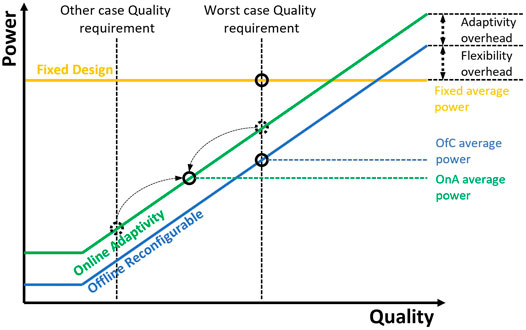
FIGURE 4. Trade-offs of fixed vs. OfC vs. OnA.

3.3 Costs of Adaptivity

The costs of adaptivity can also be categorized into OfC and OnA costs.

3.3.1 Offline Configurability Costs

Creating a flexible hardware platform entails over-designed specifications for some targeted applications, leading to an overhead for OfC (Figure 4). Examples are excessive memory, digital hardware that is optimized for speed to reach a worst-case specification instead of being optimized for leakage, analog transistors with increased drive strength, etc. These excessive specifications increase the power consumption floor, leading to higher power consumption for lower quality. Figure 4 conceptually shows how a well-designed flexible hardware platform needs to scale its power consumption with quality, over as wide a range as possible to be able to be power efficient over multiple applications. This means minimizing leakage and other constant power consumption blocks (e.g., digital clock distribution) to lower the power consumption floor as much as possible (Figure 4) while still balancing with moderate- or high-quality capabilities. An example of a flexible block is a sensor + ADC block with minimized leakage and tunable sample frequency that can reach moderate/high sample frequencies for IoT applications Xin et al. (2018, 2019). Creating scalable flexible hardware designs is a skill of its own and requires additional design time cost for a single platform, yet as mentioned before, it can then be split across multiple applications. A last contribution to the OfC costs is the tuning of the settings of a flexible hardware platform for every application, which requires optimization time costs for each application. Yet, this optimization is also needed in a non-flexible fixed design, where this optimization is carried out at design time, not at program time.

3.3.2 Added Online Adaptivity Costs

First, OnA requires an additional power-consuming awareness and control block present within the electronic system leading to OnA power overhead (Figure 4). This block both creates a design time cost and adds to the design size (e.g., chip area and FPGA usage). Moreover, designing this block requires expert knowledge of suitable environments in the application and how to efficiently detect them. Second, switching tuning knobs (TKs) online can create transient effects (e.g., batched processing with half a batch pre-processed with one setting and half a batch pre-processed with a different setting De Roose et al. (2020), delays when switching supply voltages Park et al. (2010), or clock frequencies), which might impact the quality negatively or increase power consumption. This effect is very application dependent and normally very minor. Third, adaptivity enables different TK settings in different environments, increasing the offline optimization complexity and time cost. This article proposes an approach to minimize this optimization time by introducing a generally applicable methodology.

4 Mathematical Optimization of OnA and OfC

When designing an IoT sensor node and faced with the decision of whether to implement OnA and OfC (and ultimately OnL), it is important to have all information on costs and benefits available to make an informed decision. The methodology that we adopt (Figure 5), described in the next subsections, enables us to gradually evaluate the benefits of having multiple online settings for adaptation (OnA), compared to using only one pre-configured setting (OfC). As circuits operate in multiple changing conditions, we define an environment as a small cluster of similar operating conditions. The whole range of conditions experienced by the circuit then creates several environments, and OnA intends to optimize the hardware platform for each of them.

FIGURE 5

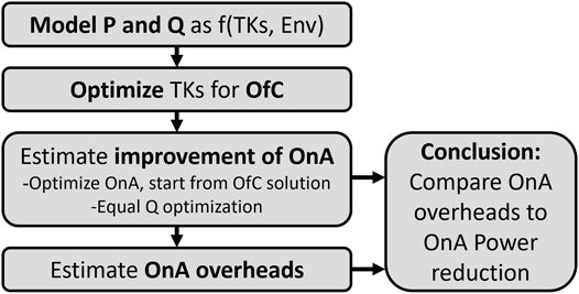
FIGURE 5. Conceptual flow of the methodology to quickly assess OnA feasibility.

The mathematical optimization aims to quickly quantify the power-related benefits of OnA compared to OfC while maintaining the same average quality requirements. This requires the ability to quantify quality, as a measure of how well the platform is performing in a specific application scenario. This could, for example, be the classification accuracy for human activity-recognition application of a smartwatch. The optimization process intends to find the best OfC, resp. OnA operating conditions for multiple quality/power trade-offs, leading to a quality/power Pareto front, as illustrated later. Going from OfC to OnA will include a power penalty, linked to the power costs of the awareness and control center required for OnA. The objective of the optimization is as such to quantify the net power savings we can expect from implementing OnA over OfC, to be able to compare this to its power penalty.

A prerequisite for adaptivity benefits is that the quality is a function of the N TKs and external factors, which define the environments. Assuming that every environment Env_i of the m experienced environments has a probability Pr_i to occur, we can express our system as

$\begin{array}{ll}\hfill Q\left(uality\right)& =f_Q\left(T{K}_1,T{K}_2,\dots ,T{K}_N,Env\right)\hfill \\ \hfill P\left(ower\right)& =f_P\left(T{K}_1,T{K}_2,\dots ,T{K}_N\right)\hfill \\ \hfill f_{Q,En{v}_x}& =f_Q\left(T{K}_1,T{K}_2,\dots ,T{K}_N,Env=x\right)\hfill \\ \hfill P{r}_{\mathit{Env,a}}& =T_{En{v}_a}/\left(T_{En{v}_a}+T_{En{v}_b}+\cdots +T_{En{v}_m}\right).\hfill \end{array}(1)$

According to this initial definition of the problem, we evaluate the OfC optimality, i.e., the achievable Q–P points when only using one optimal setting (TK₁, TK₂, … , TK_N) for the system, across all possible environments 1..m. Then, we compare OfC results to a best-case OnA, where we assume that the OnA would perfectly be able to detect the different environments (to reduce the problem complexity) and use the optimal settings for each environment individually while consuming no extra power. This enables us to evaluate if OnA can achieve power reduction compared to OfC for equal quality, without having yet to think about how OnA could be implemented and its related cost overheads. Finally, if gains are possible, we perform a real-case OnA analysis, where we consider the specific costs of the adaptivity as well. This analysis can be carried out with power estimates of the necessary blocks at first and then be refined with real circuit implementations in Section 5. This enables us to quantify the potential benefits of OnA in a real-life scenario. As such, these benefits assume that online environmental detection is perfect. Therefore, the framework proposes the most optimistic estimation, which is a quick way to decide on developing OnA further for designers. If such a development decision is taken, the environmental detection needs to be realized at a later stage, and both the power consumption of the environmental detection and the use of sub-optimal settings in wrongfully classified environments may deteriorate the results to a certain extent and further analysis would be needed. Including the optimization of power and the effect of the accuracy of the environmental detection into a more holistic optimization for OnA adds another layer of complexity that is not yet covered in this work. The whole flow to quickly estimate OnA feasibility is shown in Figure 5.

4.1 Offline Configurability Optimality

The first step is to find the optimal OfC TK setting, as a reference point to compare to OnA. For OfC, the general problem definition is to optimize the TK variables for the power objective, given a constraint of minimum target quality:

$\begin{array}{ll}\hfill \mathbf{M}\mathbf{i}\mathbf{n}\mathbf{i}\mathbf{m}\mathbf{i}\mathbf{z}\mathbf{e}\left(\mathbf{P}\right)\mathbf{w}\mathbf{i}\mathbf{t}\mathbf{h}\mathbf{Q}>{\mathbf{Q}}_{\mathbf{min}}\mathbf{f}\mathbf{o}\mathbf{r}{\mathbf{T}\mathbf{K}}_{\mathbf{1..N}}Q& =f_{Q,En{v}_a}\left(T{K}_1,T{K}_2,\dots ,T{K}_N\right)\cdot P{r}_{En{v}_a}\hfill \\ \hfill & +f_{Q,En{v}_b}\left(T{K}_1,T{K}_2,\dots ,T{K}_N\right)\cdot P{r}_{En{v}_b}+\cdots \hfill \\ \hfill & +f_{Q,En{v}_n}\left(T{K}_1,T{K}_2,\dots ,T{K}_N\right)\cdot P{r}_{En{v}_m}\hfill \\ P=f_P\left(T{K}_1,T{K}_2,\dots ,T{K}_N\right).\hfill \end{array}(2)$

Redefining the minimum target quality will lead to different solutions that all lie on a power-quality Pareto front. We first solve the problem of Eq. 2 continuously using Lagrange multipliers and later take discrete TKs in consideration:

$\begin{array}{ll}\hfill \nabla f_{\mathit{objective}}& =\lambda \nabla f_{\mathit{constraints}},f_{\mathit{constraints}}=0\hfill \\ \hfill & \to \nabla f_P=\lambda \nabla f_Q,Q-Q_{\mathit{min}}=0.\hfill \end{array}(3)$

This translates to

$\begin{array}{ll}\hfill \frac{\partial f_P}{\partial T{K}_1}& =\lambda \frac{\partial f_{Q,tot}}{\partial T{K}_1},\dots ,\frac{\partial f_P}{\partial T{K}_N}=\lambda \frac{\partial f_{Q,tot}}{\partial T{K}_N}\lambda \hfill \\ \hfill & =\frac{\frac{\partial f_P}{\partial T{K}_1}}{\frac{\partial f_{Q,tot}}{\partial T{K}_1}}=\frac{\frac{\partial f_P}{\partial T{K}_2}}{\frac{\partial f_{Q,tot}}{\partial T{K}_2}}=\dots =\frac{\frac{\partial f_P}{\partial T{K}_N}}{\frac{\partial f_{Q,tot}}{\partial T{K}_N}}.\hfill \end{array}(4)$

This means that if the ratios of the power and quality derivatives to all TKs are equal, an optimal solution is found. Intuitively, we show this in Figure 6. If the ratios are not equal, an iterative optimizer can take one step in 1 TK with a higher ratio and then subtract one step in another TK with a lower ratio to arrive at a better solution, until all partial derivative ratios converge.

FIGURE 6

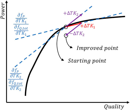
FIGURE 6. When the ratio of the power and quality derivatives to the TKs are not equal, a better solution is possible.

4.2 Best-Case Online Adaptivity Optimality

The main benefit of online adaptivity is that it allows changing the values of the TKs based on the environment. At first, we will explain an ideal scenario evaluating the potential benefits of OnA over OfC, assuming the OnA system perfectly recognizes all environments, and switch to the TK combinations designed for these environments. This means now the optimization problem has N TKs with m values for all m environments and m ⋅ N variables. The problem can be stated as

$\begin{array}{ll}\hfill & \mathbf{M}\mathbf{i}\mathbf{n}\mathbf{i}\mathbf{m}\mathbf{i}\mathbf{z}\mathbf{e}\left(\mathbf{P}\right)\mathbf{w}\mathbf{i}\mathbf{t}\mathbf{h}\mathbf{E}>{\mathbf{E}}_{\mathbf{min}}\mathbf{f}\mathbf{o}\mathbf{r}{\mathbf{T}\mathbf{K}}_{\mathbf{1a..Nn}}\hfill \\ \hfill Q& =f_{Q,En{v}_a}\left(T{K}_{1a},T{K}_{2a},\dots ,T{K}_{Na}\right)\cdot P{r}_{En{v}_a}\hfill \\ \hfill & +f_{Q,En{v}_b}\left(T{K}_{1b},T{K}_{2b},\dots ,T{K}_{Nb}\right)\cdot P{r}_{En{v}_b}+\cdots \hfill \\ \hfill & +f_{Q,En{v}_m}\left(T{K}_{1m},T{K}_{2m},\dots ,T{K}_{Nm}\right)\cdot P{r}_{En{v}_m}\hfill \\ \hfill P& =f_P\left(T{K}_{1a},T{K}_{2a},\dots ,T{K}_{Na}\right)\cdot P{r}_{En{v}_a}\hfill \\ \hfill & +f_P\left(T{K}_{1b},T{K}_{2b},\dots ,T{K}_{Nb}\right)\cdot P{r}_{En{v}_b}+\cdots \hfill \\ \hfill & +f_P\left(T{K}_{1m},T{K}_{2m},\dots ,T{K}_{Nm}\right)\cdot P{r}_{En{v}_m}.\hfill \end{array}(5)$

We can once again apply Lagrange to this optimization problem, with the same general problem statement as Eq. 3, but now with n times more variables, accounting for all environments. This leads to an equivalent of Eq. 4:

$\begin{array}{ll}\hfill \lambda & =\frac{\frac{\partial f_{P,tot}}{\partial T{K}_{1a}}}{\frac{\partial f_{Q,tot}}{\partial T{K}_{1a}}}=\frac{\frac{\partial f_{P,tot}}{\partial T{K}_{2a}}}{\frac{\partial f_{Q,tot}}{\partial T{K}_{2a}}}=\dots =\frac{\frac{\partial f_{P,tot}}{\partial T{K}_{Na}}}{\frac{\partial f_{Q,tot}}{\partial T{K}_{Na}}}=\dots =\dots =\dots =\dots \hfill \\ \hfill & =\frac{\frac{\partial f_{P,tot}}{\partial T{K}_{1m}}}{\frac{\partial f_{Q,tot}}{\partial T{K}_{1m}}}=\frac{\frac{\partial f_{P,tot}}{\partial T{K}_{2m}}}{\frac{\partial f_{Q,tot}}{\partial T{K}_{2m}}}=\dots =\frac{\frac{\partial f_{P,tot}}{\partial T{K}_{Nm}}}{\frac{\partial f_{Q,tot}}{\partial T{K}_{Nm}}}.\hfill \end{array}(6)$

This can be further elaborated as

$\begin{array}{ll}\hfill \frac{\partial f_{Q,tot}}{\partial T{K}_{1a}}& =\frac{\partial \left({\mathit{Pr}}_a\cdot f_{Q,En{v}_a}+\cdots +{\mathit{Pr}}_n\cdot f_{Q,En{v}_m}\right)}{\partial T{K}_{1a}}={\mathit{Pr}}_a\frac{\partial f_{Q,En{v}_a}}{\partial T{K}_{1a}}\hfill \\ \hfill \frac{\partial f_{P,tot}}{\partial T{K}_{1a}}& =\frac{\partial \left({\mathit{Pr}}_a\cdot f_P\left(T{K}_{En{v}_a}\right)+\cdots +{\mathit{Pr}}_n\cdot f_P\left(T{K}_{En{v}_m}\right)\right)}{\partial T{K}_{1a}}\hfill \\ \hfill & ={\mathit{Pr}}_a\frac{\partial f_P\left(T{K}_{En{v}_a}\right)}{\partial T{K}_{1a}},\hfill \end{array}(7)$

and the same goes for all other TKs. Eq. 6 now becomes

$\lambda =\frac{\frac{\partial f_P\left(T{K}_{En{v}_a}\right)}{\partial T{K}_{1a}}}{\frac{\partial f_{Q,En{v}_a}}{\partial T{K}_{1a}}}=\dots =\dots =\frac{\frac{\partial f_P\left(T{K}_{En{v}_m}\right)}{\partial T{K}_{Nm}}}{\frac{\partial f_{Q,En{v}_m}}{\partial T{K}_{Nm}}}.(8)$

Analyzing Eq. 8 essentially means that, to have an optimal point, all ratios of the power and quality derivative of all TKs in all environments need to be equal.

4.3 Mechanics of Adaptivity

The end results of the OnA and OfC optimality from Eqs 8 and 4 give us some interesting theoretical insights into the mechanics of adaptivity and the nature of environmental and TK dependencies of quality. As defined in Eq. 1, quality is a function of TKs and Env. We can further split this theoretically into a function g that is only a function of TKs, a function k that is only a function of the environment, and a cross function h:

$\begin{array}{ll}\hfill Q& =f_Q\left(TKs,Env\right)\hfill \\ \hfill & =g\left(TKs\right)+h\left(TKs,Env\right)+k\left(Env\right).\hfill \end{array}(9)$

In the solutions of OnA (Eq. 8) and OfC (Eq. 4), only the derivatives to the TKs matter, meaning that the k part of the function drops out of the equation since it is not a function of TK and, therefore, the derivative is zero. This corresponds to the influence of the environment we have no impact on using TKs. Furthermore, we can see that if the h function is zero, the solution only becomes a function of g, meaning it is only a function of the TKs, leading to identical solutions for OnA and OfC and, hence, no improvement stemming from OnA. This leads to the conclusion that the h function, namely, the different influences of TKs on the quality in different environments is the driving force of run-time adaptivity, and it stands to reason that the higher this impact, the more benefits OnA can offer over OfC. In future research, the adaptive functionality of this h function can be delved deeper upon.

4.4 Improvement of OnA

4.4.1 Estimate Improvement of OnA Upon OfC

We target an estimate of improvement from OfC to OnA based on the ratios of derivatives, as depicted in Figure 6. We will illustrate this with a simple non-optimal single TK OnA case with two environments, a and b. We estimate the possible difference in power consumption, enforcing equal quality using derivatives as a form of first-order approximation:

$\begin{array}{ll}\hfill & \left\{\begin{array}{c}\mathrm{\Delta }P\approx \partial f_P/\partial T{K}_{1a}\cdot \mathrm{\Delta }T{K}_1+\partial f_P/\partial T{K}_{1b}\cdot \mathrm{\Delta }T{K}_2\hfill \\ \mathrm{\Delta }Q\approx \partial f_Q/\partial T{K}_{1a}\cdot \mathrm{\Delta }T{K}_1+\partial f_Q/\partial T{K}_{1b}\cdot \mathrm{\Delta }T{K}_2=0\hfill \end{array}\right.\hfill \\ \hfill \mathrm{\Delta }P& \approx \left(\frac{\frac{\partial f_P}{\partial T{K}_{1b}}}{\frac{\partial f_Q}{\partial T{K}_{1b}}}-\frac{\frac{\partial f_P}{\partial T{K}_{1a}}}{\frac{\partial f_Q}{\partial T{K}_{1a}}}\right)\frac{\partial f_Q}{\partial T{K}_{1b}}\mathrm{\Delta }T{K}_{1b}.\hfill \end{array}(10)$

We will further denote the ratios of the partial derivatives by

$f_{PQ,T{K}_{Xy}}^{\prime }=\frac{\frac{\partial f_P}{\partial T{K}_{Xy}}}{\frac{\partial f_{Q,En{v}_y}}{\partial T{K}_{Xy}}}.(11)$

Here, we see the approximation of ΔP—the amount of potential power savings of OnA relative to OfC—is a function of both the partial derivatives and ΔTK_1b. Yet, as the partial derivatives are themselves also influenced by ΔTK_1b, it is not straightforward to assess the step size that can be taken on ΔTK_1b to reach the equal ratios of partial derivatives and, thus, the power optimal solution. This means the estimation cannot be performed in a single step, and instead, an iterative approach is required to update the partial derivatives, which is the concept of an optimizer. This leads us to the following methodology (Figure 5) to find a quick estimate of the improvement OnA: first, we optimize the simpler OfC solution and then use it as a starting point for an OnA optimization where the quality is kept equal. This minimizes the optimization time and allows for a fair comparison of power reduction of OnA compared to OfC, which can later be weighed against the overheads of OnA.

4.4.2 Equal-Q Optimizer

Our methodology requires optimizing the OnA solution starting from the OfC solution while keeping the quality equal. This requirement comes for easier comparison between OnA and OfC, i.e., the quality is the same and only the power varies between both approaches. This can be achieved using a constrained optimizer Jimenez et al. (2002); Sun et al. (2022). Generally, in this case, Q would be constrained to be equal to or bigger than the Q of the OfC solution, as the optimal power solution will likely be reached when lowering Q all the way to the constraint. Yet, the main requirements for our optimizer are 1) to keep Q as equal as possible for OfC and OnA and 2) to enable fast convergence toward a point that is better than OfC (if such a point exists). This is directly related to the general task of the optimizer: get quick estimates of the potential benefits of OnA. Only in a later stage, OnA is completely implemented and optimized, including the environmental detection block. We have built a custom-designed optimizer, whose goal is to make the ratio of all derivatives $f_{PQ,T{K}_{Xy}}^{\prime }$ equal and find an OnA solution close to the Pareto front in as few iterations as possible while keeping quality equal. The first step is to find $f_{PQ,T{K}_{Xy}}^{\prime }$ variables that are far away from the average value of all $f_{PQ,T{K}_{Xy}}^{\prime }$, denoted as $f_{PQ,avg}^{\prime }$, and pull them toward $f_{PQ,avg}^{\prime }$. We calculate the average ratio and compute a delta $\mathrm{\Delta }{f}_{PQ,T{K}_{Xy}}^{\prime }$ for each:

$\begin{array}{ll}\hfill f_{PQ,T{K}_{1a}}^{\prime }& \ne \dots \ne f_{PQ,T{K}_{Na}}^{\prime }\ne \dots \ne f_{PQ,T{K}_{Nm}}^{\prime }\hfill \\ \hfill f_{PQ,avg}^{\prime }& =\frac{1}{N}\frac{1}{m}\sum _{x=1}^N\sum _{y=a}^m{f}_{PQ,T{K}_{Xy}}^{\prime }\hfill \\ \hfill \mathrm{\Delta }{f}_{PQ,T{K}_{Xy}}^{\prime }& =f_{PQ,avg}^{\prime }-f_{PQ,T{K}_{Xy}}^{\prime }.\hfill \end{array}(12)$

Next, we use the derived $\mathrm{\Delta }{f}_{PQ,T{K}_{Xy}}^{\prime }$ to update the TKs to the direction that makes the $f_{PQ,T{K}_{Xy}}^{\prime }$ equal. We use a derivative of the $f_{PQ,T{K}_{Xy}}^{\prime }$ ratios to estimate how they change with changing TKs:

$\begin{array}{ll}\hfill f_{PQ,T{K}_{X}y}^{″}& =\frac{f_{PQ,T{K}_{Xy}}^{\prime }}{\partial T{K}_{Xy}}\hfill \\ \hfill \mathrm{\Delta }T{K}_{Xy}& \sim \frac{\mathrm{\Delta }{f}_{PQ,T{K}_{Xy}}^{\prime }}{f_{PQ,T{K}_{X}y}^{″}}.\hfill \end{array}(13)$

This gives the direction in which the TKs have to evolve to go toward the optimum and an estimated step size. Next, we balance out the quality of all these TK changes, so that we converge toward an OnA solution with equal quality and lower power, for easy comparison. To do this, we split the TKs into 2 groups: one group with ΔTK that increases quality and one group with ΔTK that decreases quality.

$\begin{array}{ll}\hfill & \mathrm{\Delta }Q\approx \frac{\mathrm{\Delta }{f}_{PQ,T{K}_{Xy}}^{\prime }}{f_{PQ,T{K}_{X}y}^{″}}\frac{\partial f_{Q,En{v}_y}}{\partial T{K}_{Xy}}>0\to T{K}_{Xy}^{\mathit{posQ}}\hfill \\ \hfill & \mathrm{\Delta }Q\approx \frac{\mathrm{\Delta }{f}_{PQ,T{K}_{Xy}}^{\prime }}{f_{PQ,T{K}_{X}y}^{″}}\frac{\partial f_{Q,En{v}_y}}{\partial T{K}_{Xy}}<0\to T{K}_{Xy}^{\mathit{negQ}}.\hfill \end{array}(14)$

We balance these two groups such that the overall quality change after changing all TKs remains close to zero:

$\begin{array}{ll}\hfill \mathrm{\Delta }{Q}^{\mathit{pos}}& \approx \sum _{X=1}^N\sum _{y=a}^m\frac{\partial f_{Q,En{v}_y}}{\partial T{K}_{Xy}^{\mathit{pos}}}\mathrm{\Delta }T{K}_{Xy}^{\mathit{pos}}\hfill \\ \hfill \mathrm{\Delta }{Q}^{\mathit{neg}}& \approx \sum _{X=1}^N\sum _{y=a}^m\frac{\partial f_{Q,En{v}_y}}{\partial T{K}_{Xy}^{\mathit{neg}}}\mathrm{\Delta }T{K}_{Xy}^{\mathit{neg}}\hfill \\ \hfill \mathrm{\Delta }Q& \approx \mathrm{\Delta }{Q}^{\mathit{pos}}-\mathrm{\Delta }{Q}^{\mathit{neg}}=0.\hfill \end{array}(15)$

We balance out the increase in quality with the decrease in quality by scaling all ΔTK^pos and ΔTK^neg with respective constants C^pos and C^neg.

$\begin{array}{ll}\hfill & \mathrm{\Delta }T{K}_{Xy}^{\mathit{pos}}=\frac{\mathrm{\Delta }{f}_{PQ,T{K}_{Xy}}^{\prime }}{f_{PQ,T{K}_{X}y}^{″}}{C}^{\mathit{pos}}\hfill \\ \hfill & \mathrm{\Delta }T{K}_{Xy}^{\mathit{neg}}=\frac{\mathrm{\Delta }{f}_{PQ,T{K}_{Xy}}^{\prime }}{f_{PQ,T{K}_{X}y}^{″}}{C}^{\mathit{neg}}.\hfill \end{array}(16)$

We can then calculate the value of these constants C^pos and C^neg from balancing Eq. 15:

$\begin{array}{ll}\hfill & \mathrm{\Delta }{Q}_{\mathit{est}}^{\mathit{pos}}=\sum _{X=1}^N\sum _{y=a}^m\frac{\partial f_{Q,En{v}_y}}{\partial T{K}_{Xy}^{\mathit{pos}}}\frac{\mathrm{\Delta }{f}_{PQ,T{K}_{Xy}}^{\prime }}{f_{PQ,T{K}_{X}y}^{″}}{C}^{\mathit{pos}}\hfill \\ \hfill & \mathrm{\Delta }{Q}_{\mathit{est}}^{\mathit{neg}}=\sum _{X=1}^N\sum _{y=a}^m\frac{\partial f_{Q,En{v}_y}}{\partial T{K}_{Xy}^{\mathit{neg}}}\frac{\mathrm{\Delta }{f}_{PQ,T{K}_{Xy}}^{\prime }}{f_{PQ,T{K}_{X}y}^{″}}{C}^{\mathit{neg}}.\hfill \end{array}(17)$

Also, the constant values can be related to Q_est:

$\begin{array}{ll}\hfill & C^{\mathit{pos}}=\frac{\mathrm{\Delta }{Q}_{\mathit{est}}^{\mathit{pos}}}{{\sum }_{X=1}^N{\sum }_{y=a}^m\frac{\partial f_{Q,En{v}_y}}{\partial T{K}_{Xy}^{\mathit{pos}}}\frac{\mathrm{\Delta }{f}_{PQ,T{K}_{Xy}}^{\prime }}{f_{PQ,T{K}_{X}y}^{″}}}\hfill \\ \hfill & C^{\mathit{neg}}=\frac{\mathrm{\Delta }{Q}_{\mathit{est}}^{\mathit{neg}}}{{\sum }_{X=1}^N{\sum }_{y=a}^m\frac{\partial f_{Q,En{v}_y}}{\partial T{K}_{Xy}^{\mathit{neg}}}\frac{\mathrm{\Delta }{f}_{PQ,T{K}_{Xy}}^{\prime }}{f_{PQ,T{K}_{X}y}^{″}}}.\hfill \end{array}(18)$

We know from Eq. 15 that ΔQ^pos = ΔQ^neg, but the actual value is not determined. This absolute value can be made bigger or smaller, which will increase all step sizes of the TKs. In many optimizers, the step size is large in the beginning and decreases with subsequent iterations. Because the positive and negative ΔQ are only approximations, the Q is bound to shift a little. In the next iteration, this shift can be counterbalanced by equaling the positive and negative ΔQ to the negative shift:

$\mathrm{\Delta }Q\approx \mathrm{\Delta }{Q}^{\mathit{pos}}+\mathrm{\Delta }{Q}^{\mathit{neg}}=-\mathrm{\Delta }{Q}_{\mathit{shift}}.(19)$

This optimizer is capable of changing all TKs every iteration, converging to an equal Q solution with balanced $f_{PQ}^{\prime }$s in a few iterations.

4.5 Real-Life Complications

In real-life applications, quality and power are not perfectly smooth continuous functions, which brings a few complications to the mathematical framework described above.

First, usually, a TK is not continuous and can only take a limited amount of discrete values.

$T{K}_1\in \left\{T{K}_1^1,T{K}_1^2,\dots ,T{K}_1^S\right\}.(20)$

Derivatives can as such no longer be computed with infinitesimally small increments, but only with discrete steps:

$\frac{\partial f\left(T{K}_1^i,\dots \right)}{\partial T{K}_1}=\frac{f\left(T{K}_1^{i+1},\dots \right)-f\left(T{K}_1^{i-1},\dots \right)}{2}.(21)$

Therefore, there will be a discretization error on the partial derivatives.

A second practical complication is that $f_{PQ,T{K}_{Xy}}^{\prime }$ could become negative, meaning that a decrease in power can lead to an increase in quality. These are counterintuitive TK relations, but they do exist. For example, machine learning applications that overfit can increase quality and reduce power by reducing the model size. Practically, we evolve this TK first to a more Pareto optimal point, before other optimizations take place.

Third, TKs have upper and lower bounds, dictated by the design specifications of the flexible hardware. During optimization, the optimizer might want to push the TK further, but it is blocked by the hardware platform’s tuning capabilities. The optimizer then stops optimizing the bounded TK and focuses on optimizing other TKs. Also, when approaching the bound of a TK, the optimizer takes into consideration how much room the TK has left by rescaling C_pos and C_neg. To do this, the algorithm first calculates C_pos or C_neg and checks if any ΔTK hits a TK boundary. If so, the optimizer plugs in the limiting TK change into Eq. 16 and calculates the maximum corresponding C_pos or C_neg from it. The other constant is subsequently scaled with the same diminishing factor, for balance.

Fourth, the ΔTKs for all TKs are calculated continuously and, hence, do not necessarily correspond to a discrete step that this TK can precisely take. Therefore, each TK is changed to the nearest lower discrete TK step it can take. Because ΔTK could potentially be lower than the discretization step (hence, TK would never change), the continuous value subtracted by the taken discrete TK step is stored and added to the ΔTK of the next iteration.

All these complications deteriorate the operation of the optimizer in real-use cases, but they do not block the optimizer from functioning, as we will show in the following parts of this article.

4.6 Theoretical Test Case

To test the convergence speed and the resilience to discretization and TL limits of the equal-Q optimization algorithms, we first deploy it on a simple conceptual use case defined by a mathematical continuous function where increased power consumption yields less and less increase in quality, with two TKs and two environments:

$\begin{array}{ll}\hfill f_Q& =5\sqrt{T{K}_1}\cdot En{v}^4+2\sqrt{T{K}_2}\cdot En{v}^4+3\cdot Env\hfill \\ \hfill f_P& =2T{K}_1^2+5T{K}_2^2\hfill \\ \hfill 0& <T{K}_1<\mathrm{10,0}<T{K}_2<10Env\in \left\{\mathrm{1,2}\right\}.\hfill \end{array}(22)$

In Figure 7, the achievable Pareto front for OfC operation is plotted in blue, and the best-case OnA Pareto front is in orange. Here, both are obtained by evaluating all possible settings with a brute-force method, as a way to establish a ground truth in this test. Across the different subplots in Figures 7A–C, results are plotted for increasing TK discretization, only allowing limited and discrete TK values. This results in a Pareto front with a coarser granularity and also makes the optimization more difficult.

FIGURE 7

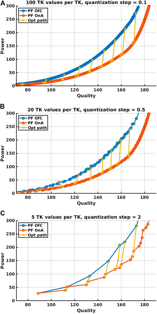
FIGURE 7. Applying the optimization algorithm of Section 4 to a theoretical use case, with increasing discretization step size.

It is possible to analytically solve the optimization of these OfC and OnA systems, given the mathematics described in the previous section. However, what interests us is to deploy and evaluate the optimization methodology presented in Section 4, in terms of convergence speed, ability to keep equal quality, and resilience to discretization. The basic idea we apply is to start from an OfC solution and find a good estimate of the power benefits available when using OnA using as few function evaluations as possible.

To this end, the yellow lines in each subplot show the optimization steps, starting from a few points on the OfC Pareto front. As can be seen, after one optimization iteration, the solution has reached (almost or exactly) the OnA Pareto front with a very similar quality, showing the high efficiency of the optimization algorithm in a theoretical case. Furthermore, bigger discretization steps (as shown in Figures 7B, C) are harder for the optimizer with solutions diverging more from the original quality but do not block its proper functioning.

5 Practical Use Cases

We selected a few state-of-the-art works from the literature, which have successfully implemented adaptivity in their respective applications. These will be used as case studies to go through the steps of the proposed quick assessment methodology (Figure 5). The selection encompasses a case with ECG signal compression Ieong et al. (2017) that can be used for wearable heart rate monitoring, a use case with a battery-powered wireless video node recognizing people Cao et al. (2017), and our own previous work on sound-based machine anomaly detection De Roose et al. (n d).

5.1 Adaptive Temporal Decimation on ECG Signals

The first use case, in the work of Ieong et al. (2017), is an ECG signal compression application. The ECG sensor node adaptively decimates the signal first and subsequently uses wavelet shrinkage and Huffman encoding to compress the signal before storing or transmitting it (see Figure 8, based on Figure 1 of the original work by Ieong et al. (2017)).

FIGURE 8

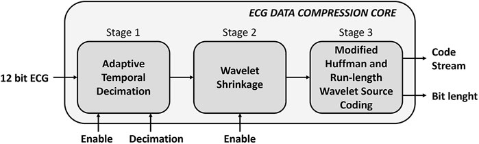
FIGURE 8. ECG signal compression overview, based on Figure 1 of the work of Ieong et al. (2017).

5.1.1 Application Details

In this application, the environmental influence is the instantaneous frequency of the input ECG signal. The ECG signal consists of the faster QRS wave and the longer slower P/T wave, with a periodicity of 0.3–3 s Ieong et al. (2017), leading to some very-high-frequency adaptivity.

The signal degradation is lower when subsampling the PT part of the signal, compared to subsampling the QRS waves, as is visualized in Figure 2 of the original work by Ieong et al. (2017). Therefore, we focus on the adaptive decimation part, as this is where the adaptivity lies. We do not focus on wavelet shrinkage or the Huffman encoding.

Under this assumption, the only TK (Table 1) is the subsampling rate, being able to sample 1, 2, 4, 16, or 32 times slower than the original input sample frequency of 360 Hz.

TABLE 1

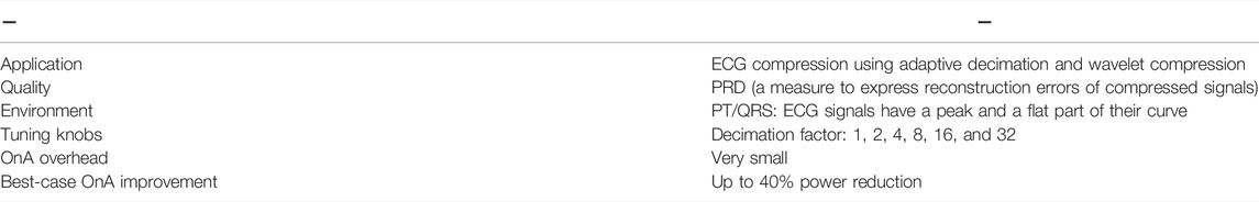
TABLE 1. Overview of adaptivity in the ECG signal compression study by Ieong et al. (2017).

5.1.2 Methodology

5.1.2.1 Power/Quality Model

Using Figure 2 of the original work by Ieong et al. (2017), we are able to build a power/quality model of adaptive temporal decimation by isolating the PRD increase from either the QRS part or the PT part of the waveform. Once isolated, they are a function of the decimation factor in each environment, which can take five discrete factors, and the complete PRD can be calculated by combining the two parts of the PRD again. The power is expressed in data rate, which translates to power when taking the TX energy/bit cost into account. The quality is defined as “1-PRD,” with PRD being the percentage root-mean-square distortion, which is an expression of the reconstruction error of the signal:

$PRD=\frac{\sqrt{\frac{\sum {\left(x_i-{\widehat{x}}_i\right)}^2}{N}}}{\sqrt{\frac{\sum x_i^2}{N}}},(23)$

with x_i being the original signal and ${\widehat{x}}_i$ the reconstructed signal.

5.1.2.2 OfC Optimization and OnA Improvement

Figure 9 shows achievable OfC solutions in blue and OnA solutions in orange. We let the optimizer once again start from each OfC solution, converging to an OnA solution. In purple, we show the solutions picked in the original work, showing that the original work finds not only Pareto optimal OnA solutions but also some non-optimal solutions. Our optimization method consistently finds optimal OnA settings. We see that up to a maximum of 40% power can be saved by adaptively changing decimation rates between QRS and P/T parts of the ECG signal, when allowing some minimal signal deterioration.

FIGURE 9

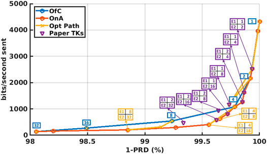
FIGURE 9. Adaptive temporal decimation power benefits from adaptivity.

5.1.2.3 OnA Overheads

The flexibility to switch decimation rates requires an overdesign of the ADC sample speed. Yet, due to the very low sample frequencies, the related cost is negligible. Also, the recognition of the P/T and QRS environment can be implemented at a low cost, using a single MAD (mean absolute deviation) feature and a threshold comparing the original feature to a set fraction of the MAD, which is negligible compared to the cost of wavelet calculations and the Huffman encoding.

5.1.2.4 Conclusion

Even though the benefits of OnA are quite limited, because of the absolute minimal power consumption of the added OnA blocks, it is clear that adaptivity is the best solution for this application.

5.2 Wireless Video Node

The second use case Cao et al. (2017) entails a wireless video sensor node, with in situ data processing abilities. A battery-charged video sensor node recognizes the presence of humans in its field of view and sends this information wirelessly to a base station.

5.2.1 Application Details

The application’s environmental influence is the path loss (PL) of the signal sent from the video node to the base station. When the PL degrades, the amplifier gain must be higher, increasing the energy per transmitted bit, hence driving the sensor node toward solutions with lower radio frequency (RF) data rates and more embedded processing.

The application has 2 TKs (Table 2). The first TK is the algorithm (Alg): a support vector machine (SVM), a naive Bayes classifier, or a tree-based classifier. The second TK is the embedded processing depth (PD), as shown in Figure 10 (based on Figure 3 from the original work). The PD can take three values, with increasingly more computation and generally increasingly less data output. It increases the amount of embedded processing costs computational power, but reduces the amount of data that has to be sent to the base station via RF, reducing the RF power. With changing energy/bit due to the environment, the amount of embedded processing shifts to create an overall minimum of power:

$\begin{array}{ll}\hfill f_Q& =f\left(Alg\right)\hfill \\ \hfill f_P& =P_{\mathit{processing}}\left(Alg,PD\right)+P_{RF}\left(Alg,PD,Env\right)\hfill \\ \hfill P_{RF}& =Datarat{e}_{RF}\left(Alg,PD\right)\cdot Energy/bit\left(AmpGain\left(Env\right)\right).\hfill \end{array}(24)$

TABLE 2

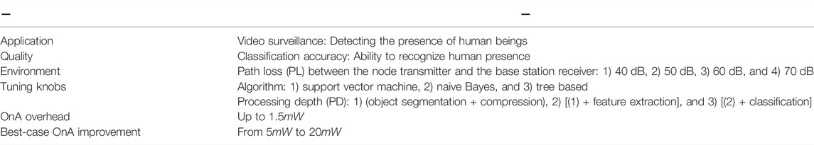
TABLE 2. Overview of flexible TKs in the wireless video node Cao et al. (2017).

FIGURE 10

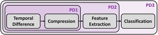
FIGURE 10. Wireless video node processing structure, based on Figure 3 of the work of Cao et al. (2017).

Normally, power consumption is only a function of the TKs and not a function of the environment. Yet, here, power is also a function of a (hidden) TK, the amplifier gain, which reacts adaptively to the PL, creating a functional relationship between power and environment. The same optimization principles still hold when the power also becomes a (pseudo)function of the environment.

5.2.2 Methodology

5.2.2.1 Power/Quality Model

Using the data from the work of Cao et al. (2017) at 10⁻⁸ BER, we constructed a power/quality model of the application in the function of the TKs and the environmental PL.

5.2.2.2 OfC Optimization and OnA Improvement

The Pareto fronts of both OfC and OnA are calculated through (brute force) optimization. Figure 11 shows the OfC and OnA power-accuracy curve achievable with the available TKs, assuming all 4 PL environments are equally probable in the use case. The figure also highlights the (trivial) optimization paths for OnA optimization starting from all OfC points using the introduced equal-Q optimizer. The lowest power OfC point is a local minimum, as can be seen from figure 17 of the original work, and therefore, the optimizer does not optimize further. Looking at the distance between the orange and blue curves in this graph (Figure 11), it is apparent that the power consumption can be reduced by about 0.5–2 mJ/frame by enabling OnA. Better solutions than the ones proposed in the article are available in the mid-accuracy range, which is achieved by allowing to switch algorithms online using OnA.

FIGURE 11

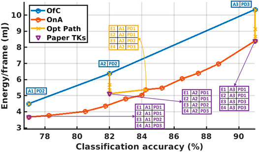
FIGURE 11. Wireless video node: Ofc vs. best-case OnA power-quality Pareto fronts, with quality being the detection accuracy of people in the camera and power expressed in mJ/frame.

5.2.2.3 OnA Overheads

The costs of OfC are the support for multiple algorithms in the same sensor node, creating a larger design and more leakage. The costs of OnA are mainly related to PL estimation. PL estimation can be carried out at the base station, inferring limited communication overhead, as assumed in the work of Cao et al. (2017). The alternative is to estimate the PL on the system itself. From the literature, the power cost can be estimated to be 2.34 mW with an analog implementation Wang et al. (2011) or 1.5 mW with a digital implementation Saalfeld et al. (2018).

5.2.2.4 Conclusion

The aforementioned costs (1.5–2.3 mW for on-chip PL detection) can be compared to the 0.5–2 mJ/frame@10frames/s of power savings gained using adaptivity, corresponding to 5–20 mW of savings. It can, hence, be concluded that OnA has clear benefits over OfC in this application.

5.3 Anomaly Detection

The last application we use as a case study is acoustic anomaly detection in industrial machines De Roose et al. (n d). The principle is to place a microphone next to a machine and use audio data to detect any anomaly/problem on the machine using a machine-learning-based anomaly detector.

5.3.1 Application Details

The anomaly detector is shown in Figure 12. Feature extraction is based on the Mel features calculated from the sound data through fast Fourier transform (FFT). The FFT is calculated at regular intervals, and the current Mel features are combined with Mel features from previous FFTs. These features are subsequently fed to an auto-encoding neural network, which is trained to recreate the network’s input at the network’s output. When the inputs and outputs are very different, the network fails to represent the data and an anomaly is detected Purohit et al. (2019); De Roose et al. (n d).

FIGURE 12

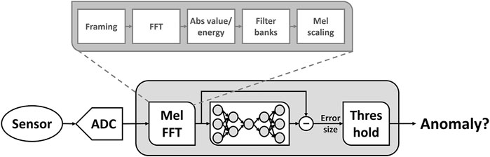
FIGURE 12. Main architecture of the work of De Roose et al. (n d).

The TKs defined in this work are shown in Table 3. They are the sampling frequency of the incoming acoustic signal, N_FFT, the Hop length, the number of Mel features (MF) extracted, the number of frames combined to create the complete input features, and the size of the fully connected neural network with relu activations, expressed as (#melFeat ⋅ #frames) × 64 × 64 × 8 × 64 × 64 × (#melFeat ⋅ #frames). The number of nodes of each internal layer (64 × 64 × 8 × 64 × 64) can be reduced by a factor of 2, 4, or 8.

TABLE 3

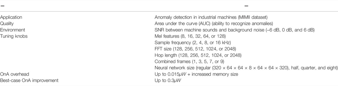
TABLE 3. Overview of flexible TKs in the anomaly detection study by De Roose et al. (n d).

The adaptive sound-based anomaly detection Purohit et al. (2019); De Roose et al. (n d) uses the SNR of the machine sounds to the factory background noise as the drive for adaptivity. The system is trained with the MIMII dataset Purohit et al. (2019), where the machine sound and background noises are mixed with each other at 3 different SNR levels: −6 dB, 0 dB, and 6 dB. The task of finding anomalies becomes harder as the SNR decreases.

5.3.2 Methodology

5.3.2.1 Power/Quality Model

The optimization of the anomaly detection is based on the area under (the ROC) curve as a quality measure, and a power model, which estimates the power by counting the number of additions, multiplications, and memory operations per second and multiplying it by, respectively, the relative energy per additions, multiplications, and memory operations, as reported in the study by Horowitz (2014). The operations required for sound-based anomaly detection are mainly in the mel feature (MF) calculation algorithm and neural network (NN) execution. The number of operations is expressed as a function of the different TKs:

$\begin{array}{ll}\hfill f_A& =f\left(N_{\mathit{mel}},f_s,N_{\mathit{FFT}},L_{\mathit{hop}},N_{\mathit{frames}},siz{e}_{NN}\right)\hfill \\ \hfill f_P& =\left[E_{MF}\left(N_{\mathit{mel}},N_{\mathit{FFT}}\right)+E_{NN}\left(N_{\mathit{mel}},N_{\mathit{frames}},siz{e}_{NN}\right)\right]\ast \left(f_s/L_{\mathit{hop}}\right)\hfill \\ \hfill E_{MF}& =Ad{d}_{MF}\ast \frac{Energy}{Add}+Mul{t}_{MF}\ast \frac{Energy}{Mult}+MemO{p}_{MF}\ast \frac{Energy}{MemOp}\hfill \\ \hfill E_{NN}& =Ad{d}_{NN}\ast \frac{Energy}{Add}+Mul{t}_{NN}\ast \frac{Energy}{Mult}+MemO{p}_{NN}\ast \frac{Energy}{MemOp}.\hfill \end{array}(25)$

5.3.2.2 OfC Optimization and OnA Improvement

We can apply the optimizer proposed in this paper to start optimization from OfC Pareto points to improve beyond OfC, as shown in Figure 13.

FIGURE 13

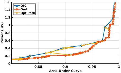
FIGURE 13. Anomaly detection power benefits from adaptivity.

One of the main problems with the previous work was the slow evaluation time, due to the training of a neural network. The brute-force method in the study by De Roose et al. (n d) required hundreds of evaluations for each Pareto point. This prevented the exploration of a wide variety of tuning knob settings. With the method provided in this article, however, we found a solution using only tens of evaluations. This allows to increase the number of TK settings and environments. In turn, this creates new, more optimal settings with a better power-quality trade-off, as shown in Figure 14. In particular, the power consumption can be decreased by a factor of 5 and more, due to the ability to converge faster and, thus, allow more tuning knob options.

FIGURE 14

FIGURE 14. Anomaly detection power benefits from adaptivity, when widening the amount of TK options due to a more efficient optimizer.

5.3.2.3 OnA Overhead

The power consumption overhead of OfC comes from increased leakage due to larger memories required to fit the maximum-sized FFT intermediate results and the maximum-sized neural network weights. These leakages can be mitigated by power gating unused memory when using lower-performance settings. The power consumption impact of OnA stems from the power cost of the environmental detection block, and the memory leakage cost to store multiple NN models optimized for different TKs, to be able to switch between them at run time for different environments.

5.3.2.4 Conclusion

The overheads have to be weighed against the results from Figure 14, indicating power benefits for OnA of about 300 nW in some parts of the Pareto front. Although the work of De Roose et al. (n d) demonstrates that the self-awareness block consumes less than 15 nW, it is likely that the increase in leakage due to the additional extra memory requirements overshadows the benefits of OnA relative to OfC. For this reason, it is crucial to enable OnA to reuse the same NN models for different TKs to mitigate this cost or to stick with the simpler OfC solution.

6 Conclusion

In this article, we discussed in detail the opportunities stemming from offline reconfigurability (OfC) and online adaptivity (OnA). The benefits of OfC and flexible hardware platforms are mainly business related, reducing design and production costs, with a potential overhead in terms of power efficiency. The benefits of OnA, on the other hand, are mainly power efficiency related, due to its ability to adaptively select settings to meet a minimum required quality level in different environments. Yet, OnA comes with additional costs, in the form of 1) additional power consumption to drive the adaptivity and 2) increased optimization complexity. This article creates a roadmap to quickly and efficiently evaluate if OnA saves more power than it costs and whether it is to be preferred over OfC for specific use cases. The main contributions are insights into the adaptivity mechanics; an OfC–OnA optimization protocol with a fast optimizer to deal with many OnA tuning knobs; and its deployment to theoretical and practical use cases.

Data Availability Statement

The original contributions presented in the study are included in the article/Supplementary Material; further inquiries can be directed to the corresponding author.

Author Contributions

JDR coined the idea of an analysis of adaptivity on a broader level and developed the optimization mathematics and following insights into adaptivity as a concept. JDR also worked out the case studies presented in this work. MA helped place the work in the broader literature and helped in editing the manuscript. MV is the guiding professor and provided feedback, both on the fundamental research and the writing of the manuscript.

Funding

This research received funding from the Flemish Government (AI Research Program), EU ERC under grant agreement ERC-2016-STG-715037 and the ETF project ISAAC.

Conflict of Interest

The authors declare that the research was conducted in the absence of any commercial or financial relationships that could be construed as a potential conflict of interest.

Publisher’s Note

All claims expressed in this article are solely those of the authors and do not necessarily represent those of their affiliated organizations, or those of the publisher, the editors, and the reviewers. Any product that may be evaluated in this article, or claim that may be made by its manufacturer, is not guaranteed or endorsed by the publisher.

References

Alioto, M., De, V., and Marongiu, A. (2018). Energy-Quality Scalable Integrated Circuits and Systems: Continuing Energy Scaling in the Twilight of Moore's Law. IEEE J. Emerg. Sel. Top. Circuits Syst. 8, 653–678. doi:10.1109/JETCAS.2018.2881461

CrossRef Full Text | Google Scholar

Alioto, M. (2018). Enabling the Internet of Things: From Integrated Circuits to Integrated Systems. 1st edn. Berlin: Springer Publishing Company, Incorporated.

Google Scholar

Alioto, M. (2017). “Energy-Quality Scalable Adaptive VLSI Circuits and Systems Beyond Approximate Computing,” in Design, Automation Test in Europe Conference Exhibition (DATE), 2017, Lausanne, March 27-31, 2017127–132. doi:10.23919/DATE.2017.7926970

CrossRef Full Text | Google Scholar

Andraud, M., and Verhelst, M. (2018). “From On-Chip Self-Healing to Self-Adaptivity in Analog/RF ICs: Challenges and Opportunities,” in 2018 IEEE 24th International Symposium on On-Line Testing And Robust System Design (IOLTS), Platja d’Aro, Costa Brava, July 2–4, 2018, 131–134. doi:10.1109/IOLTS.2018.8474078

CrossRef Full Text | Google Scholar

Anzanpour, A., Azimi, I., Gotzinger, M., Rahmani, A. M., TaheriNejad, N., Liljeberg, P., et al. (2017). “Self-Awareness in Remote Health Monitoring Systems Using Wearable Electronics,” in Design, Automation Test in Europe Conference Exhibition (DATE), 2017, Lausanne, March 27–31, 1056–1061. doi:10.23919/DATE.2017.7927146

CrossRef Full Text | Google Scholar

Badami, K., Steven, L., Wannes, M., and Marian, V. (2015). “Context-Aware Hierarchical Information-Sensing in a 6 μ W 90nm CMOS Voice Activity Detector,” in Proc. of IEEE International Solid-State Circuits Conference, San Francisco, February 22-26, 2015, 430–432.

Google Scholar

Banerjee, D., Muldrey, B., Wang, X., Sen, S., and Chatterjee, A. (2017). Self-learning RF Receiver Systems: Process Aware Real-Time Adaptation to Channel Conditions for Low Power Operation. IEEE Trans. Circuits Syst. I 64, 195–207. doi:10.1109/tcsi.2016.2608962

CrossRef Full Text | Google Scholar

Cao, N., Nasir, S. B., Sen, S., and Raychowdhury, A. (2017). Self-Optimizing Iot Wireless Video Sensor Node with In-Situ Data Analytics and Context-Driven Energy-Aware Real-Time Adaptation. IEEE Trans. Circuits Syst. I 64, 2470–2480. doi:10.1109/tcsi.2017.2716358

CrossRef Full Text | Google Scholar

Chatterjee, B., Cao, N., Raychowdhury, A., and Sen, S. (2019). Context-Aware Intelligence in Resource-Constrained IoT Nodes: Opportunities and Challenges. IEEE Des. Test. 36, 7–40. doi:10.1109/MDAT.2019.2899334

CrossRef Full Text | Google Scholar

[Dataset] Chatterjee, B., Seo, D.-H., Chakraborty, S., Avlani, S., Jiang, X., Zhang, H., et al. (2020). Context-Aware Collaborative Intelligence with Spatio-Temporal In-Sensor-Analytics for Efficient Communication in a Large-Area IoT Testbed. IEEE Internet Things J. 8 (8), 6800–6814. doi:10.1109/JIOT.2020.3036087

CrossRef Full Text | Google Scholar

Chen, F., Chandrakasan, A. P., and Stojanovic, V. M. (2012). Design and Analysis of a Hardware-Efficient Compressed Sensing Architecture for Data Compression in Wireless Sensors. IEEE J. Solid-State Circuits 47, 744–756. doi:10.1109/JSSC.2011.2179451

CrossRef Full Text | Google Scholar

De Roose, J., Dekkers, G., Boons, B., and Verhelst, M. (n d). Adaflow: Optimization Flow for Sensor Nodes with Online Adaptive Processing. ACM Transactions on Embedded Computing Systems (TECS). Under Revision.

Google Scholar

De Roose, J., Xin, H., Hallawa, A., Ascheid, G., Harpe, P. J. A., and Verhelst, M. (2020). Flexible, Self-Adaptive Sense-And-Compress SoC for Sub-microwatt Always-On Sensory Recording. IEEE Solid-State Circuits Lett. 3, 362–365. doi:10.1109/LSSC.2020.3018382

CrossRef Full Text | Google Scholar

Eldash, O., Khalil, K., and Bayoumi, M. (2017). “On On-Chip Intelligence Paradigms,” in 2017 IEEE 30th Canadian Conference on Electrical and Computer Engineering (CCECE), Windsor, March 30, 2017, 1–6. doi:10.1109/CCECE.2017.7946728

CrossRef Full Text | Google Scholar

Fallahzadeh, R., Ortiz, J. P., and Ghasemzadeh, H. (2017). “Adaptive Compressed Sensing at the Fingertip of Internet-Of-Things Sensors: An Ultra-low Power Activity Recognition,” in Design, Automation Test in Europe Conference Exhibition (DATE), 2017, Lausanne, March 27–31, 2017, 996–1001. doi:10.23919/DATE.2017.7927136

CrossRef Full Text | Google Scholar

Giraldo, J. S. P., O'Connor, C., and Verhelst, M. (2019). “Efficient Keyword Spotting through Hardware-Aware Conditional Execution of Deep Neural Networks,” in 2019 IEEE/ACS 16th International Conference on Computer Systems and Applications (AICCSA), Abu Dhabi, November 3–7, 2019, 1–8. doi:10.1109/AICCSA47632.2019.9035275

CrossRef Full Text | Google Scholar

Gligor, M., Fournel, N., and Petrot, F. (2009). “Adaptive Dynamic Voltage and Frequency Scaling Algorithm for Symmetric Multiprocessor Architecture,” in 2009 12th Euromicro Conference on Digital System Design, Architectures, Methods and Tools, Patras, August 27–29, 2009, 613–616. doi:10.1109/DSD.2009.155

CrossRef Full Text | Google Scholar

Horowitz, M. (2014). “1.1 Computing's Energy Problem (And What We Can Do about it),” in 2014 IEEE International Solid-State Circuits Conference Digest of Technical Papers (ISSCC), San Fransisco, February 9–13, 2014, 10–14. doi:10.1109/ISSCC.2014.6757323

CrossRef Full Text | Google Scholar

Huang, Y.-J., Tzeng, T.-H., Lin, T.-W., Huang, C.-W., Yen, P.-W., Kuo, P.-H., et al. (2014). A Self-Powered CMOS Reconfigurable Multi-Sensor SoC for Biomedical Applications. IEEE J. Solid-State Circuits 49, 851–866. doi:10.1109/jssc.2013.2297392

CrossRef Full Text | Google Scholar

Ieong, C.-I., Li, M., Law, M.-K., Mak, P.-I., Vai, M. I., and Martins, R. P. (2017). A 0.45 V 147-375 nW ECG Compression Processor with Wavelet Shrinkage and Adaptive Temporal Decimation Architectures. IEEE Trans. VLSI Syst. 25, 1307–1319. doi:10.1109/TVLSI.2016.2638826

CrossRef Full Text | Google Scholar

[Dataset] IOT Analytics (2020). State of the Iot 2020: 12 Billion IoT Connections, Surpassing Non-IoT for the First Time. Available at: https://iot-analytics.com/state-of-the-iot-2020-12-billion-iot-connections-surpassing-non-iot-for-the-first-time/

Google Scholar

Jimenez, F., Gomez-Skarmeta, A. F., Sanchez, G., and Deb, K. (2002). “An Evolutionary Algorithm for Constrained Multi-Objective Optimization,” in Proceedings of the 2002 Congress on Evolutionary Computation. CEC’02 (Cat. No.02TH8600), Honolulu, march 12–17, 2002 2, 1133–1138. doi:10.1109/CEC.2002.1004402

CrossRef Full Text | Google Scholar

Lee, S., Shi, C., Wang, J., Sanabria, S., Osman, H., Hu, J., et al. (2018). A Built-In Self-Test and In Situ Analog Circuit Optimization Platform. IEEE Trans. Circuits Systems-I Regul. Pap. 65 (10), 3445–3458. doi:10.1109/TCSI.2018.2805641

CrossRef Full Text | Google Scholar

[Dataset] Mahmood, N. H., Böcker, S., Munari, A., Clazzer, F., Moerman, I., Mikhaylov, K., et al. (2020). White Paper on Critical and Massive Machine Type Communication towards 6g. Preprint. doi:10.48550/ARXIV.2004.14146

CrossRef Full Text | Google Scholar

Maroudas, E., Lalis, S., Bellas, N., and Antonopoulos, C. D. (2021). Exploring the Potential of Context-Aware Dynamic CPU Undervolting. New York, NY, USA: Association for Computing Machinery, 73–82.

Google Scholar

Meghdadi, M., and Bakhtiar, S. (2014). Two-Dimensional Multi-Parameter Adaptation of Noise, Linearity, and Power Consumption in Wireless Receivers. IEEE Trans. Circuits Syst. I 61, 2433–2443. doi:10.1109/tcsi.2014.2304654

CrossRef Full Text | Google Scholar

Moons, B., and Verhelst, M. (2014). Energy-Efficiency and Accuracy of Stochastic Computing Circuits in Emerging Technologies. IEEE J. Emerg. Sel. Top. Circuits Syst. 4, 475–486. doi:10.1109/JETCAS.2014.2361070

CrossRef Full Text | Google Scholar

Park, J., Shin, D., Chang, N., and Pedram, M. (2010). “Accurate Modeling and Calculation of Delay and Energy Overheads of Dynamic Voltage Scaling in Modern High-Performance Microprocessors,” in 2010 ACM/IEEE International Symposium on Low-Power Electronics and Design (ISLPED), Austin, August 18–20, 2010, 419–424. doi:10.1145/1840845.1840938

CrossRef Full Text | Google Scholar

Peluso, V., and Calimera, A. (2019). “Energy-accuracy Scalable Deep Convolutional Neural Networks: A Pareto Analysis,” in VLSI-SoC: Design and Engineering of Electronics Systems Based on New Computing Paradigms. Editors N. Bombieri, G. Pravadelli, M. Fujita, T. Austin, and R. Reis (Cham: Springer International Publishing), 107–127. doi:10.1007/978-3-030-23425-6_6

CrossRef Full Text | Google Scholar

Purohit, H., Tanabe, R., Ichige, K., Endo, T., Nikaido, Y., Suefusa, K., et al. (2019). MIMII Dataset: Sound Dataset for Malfunctioning Industrial Machine Investigation and Inspection. arXiv preprint arXiv:1909.09347.

Google Scholar

[Dataset] Rizzo, R. (2019). Energy-accuracy Scaling in Digital Ics: Static and Adaptive Design Methods and Tools. Doctoral Thesis. politecnico de Torino.

Google Scholar

Saalfeld, T., Piwczyk, T., Wunderlich, R., and Heinen, S. (2018). A Digital Receiver Signal Strength Detector for Multi-Standard Low-IF Receivers. Adv. Radio Sci. 16, 51–57. doi:10.5194/ars-16-51-2018

CrossRef Full Text | Google Scholar

Sen, S., Banerjee, D., Verhelst, M., and Chatterjee, A. (2012). A Power-Scalable Channel-Adaptive Wireless Receiver Based on Built-In Orthogonally Tunable LNA. IEEE Trans. Circuits Syst. I 59, 946–957. doi:10.1109/tcsi.2012.2191314

CrossRef Full Text | Google Scholar

Sen, S., Natarajan, V., Devarakond, S., and Chatterjee, A. (2014). Process-Variation Tolerant Channel-Adaptive Virtually Zero-Margin Low-Power Wireless Receiver Systems. IEEE Trans. Comput.-Aided Des. Integr. Circuits Syst. 33, 1764–1777. doi:10.1109/tcad.2014.2358535

CrossRef Full Text | Google Scholar

Shafique, K., Khawaja, B. A., Sabir, F., Qazi, S., and Mustaqim, M. (2020). Internet of Things (Iot) for Next-Generation Smart Systems: A Review of Current Challenges, Future Trends and Prospects for Emerging 5g-Iot Scenarios. IEEE Access 8, 23022–23040. doi:10.1109/ACCESS.2020.2970118

CrossRef Full Text | Google Scholar

Sun, Z., Ren, H., Yen, G. G., Chen, T., Wu, J., An, H., et al. (2022). An Evolutionary Algorithm with Constraint Relaxation Strategy for Highly Constrained Multiobjective Optimization. IEEE Trans. Cybern. 1, 1–15. doi:10.1109/TCYB.2022.3151974

CrossRef Full Text | Google Scholar

Teerapittayanon, S., McDanel, B., and Kung, H. T. (2016). “Branchynet: Fast Inference via Early Exiting from Deep Neural Networks,” in 2016 23rd International Conference on Pattern Recognition (ICPR), Cancun, December 4–8, 2016, 2464–2469. doi:10.1109/ICPR.2016.7900006

CrossRef Full Text | Google Scholar

Teo, J. H., Cheng, S., and Alioto, M. (2020). Low-Energy Voice Activity Detection via Energy-Quality Scaling from Data Conversion to Machine Learning. IEEE Trans. Circuits Syst. I 67, 1378–1388. doi:10.1109/TCSI.2019.2960843

CrossRef Full Text | Google Scholar

Trakimas, M., and Sonkusale, S. R. (2011). An Adaptive Resolution Asynchronous ADC Architecture for Data Compression in Energy Constrained Sensing Applications. IEEE Trans. Circuits Syst. I 58, 921–934. doi:10.1109/TCSI.2010.2092132

CrossRef Full Text | Google Scholar

Wang, K., Gu, J., Lim, K. M., Yan, J., Lim, W. M., Cao, X., et al. (2011). “A CMOS Low-Power Receiving Signal Strength Indicator Using Weak-Inversion Limiting Amplifiers,” in 2011 IEEE International Conference of Electron Devices and Solid-State Circuits, Hong Kong, November 17–18, 2011, 1–2. doi:10.1109/EDSSC.2011.6117642

CrossRef Full Text | Google Scholar

Xin, H., Andraud, M., Baltus, P., Cantatore, E., and Harpe, P. (2018). “A 0.1nW −1µW All-Dynamic Capacitance-To-Digital Converter with Power/Speed/Capacitance Scalability,” in ESSCIRC 2018 - IEEE 44th European Solid State Circuits Conference (ESSCIRC), Dresden, September 3-6, 2018, 18–21. doi:10.1109/ESSCIRC.2018.8494321

CrossRef Full Text | Google Scholar

Xin, H., Andraud, M., Baltus, P., Cantatore, E., and Harpe, P. (2019). “A 0.34-571nw All-Dynamic Versatile Sensor Interface for Temperature, Capacitance, and Resistance Sensing,” in ESSCIRC 2019 - IEEE 45th European Solid State Circuits Conference (ESSCIRC), 161–164. doi:10.1109/ESSCIRC.2019.8902918

CrossRef Full Text | Google Scholar