Monitoring and modelling of butyltin compounds in Finnish inland lake

1 Introduction

Organotin compounds (OTCs) have been widely used in different industrial applications for over 50 years (Champ and Seligman 1996; Fent 1996; Hoch 2001; Dubalska et al., 2013). Due to their versatile properties OTCs have been utilized as biocides, pesticides, wood preservatives, catalysts, and stabilizing agents in polymers. But OTCs, especially tri-substituted ones, are toxic to a variety of aquatic organisms (Bryan and Gibbs 1991; Hoch 2001; Aguilar-Martinez et al., 2008a) and the hazardousness of tributyltin (TBT) for aquatic organisms appears even below ng L⁻¹ concentration levels (Bryan and Gibbs 1991; Dı́ez et al., 2002). The Annual Average Environmental Quality Standard (AA-EQS) concentration for TBT is 0.2 ng L⁻¹ and the maximum allowable concentration (MAC-EQS) is 1.5 ng L⁻¹ (European Council, 2008). Considering its low aquatic concentrations, the detection of OTCs requires sensitive analytical techniques.

Estimation of the sources and transport of BTCs and especially TBT difficult. BTCs are highly attracted by solid particles or bioaccumulated and are commonly found in sediment samples or aquatic organisms (Page et al., 1996; Harino et al., 1998; Berto et al., 2007; Cole et al., 2018). They also have long a transformation chain from tertbutyltin (TeBT) to MBT (TeBT→TBT→DBT→MBT). Degradation occurs via loss of a butyl group caused mainly by photolysis (ultraviolet UV irradiation), bacteria (biological cleavage), or nucleophile or electrophile reagents (chemical cleavage) (Hoch 2001). Due to their low solubility, BTCs tend to attach to particles and sediment where degradation is slow, occurring over several weeks or even years. The process is considerably slower in anaerobic than in aerobic sediments (Seligman et al., 1986). Sediments are still not a permanent sink for OTCs, however, since due to mechanical resuspension they can dissolve back into the water column (Page et al., 1996; Filipkowska et al., 2014). Particles can drift to unpolluted sites where, e.g., tidal fluxes and dredging can cause resuspension of BTCs, favoring the release of DBT over TBT (Dowson et al., 1993; Berto et al., 2007). In shallow lakes even waves created by storms and big boats can cause resuspension. Therefore, the dispersion of BTCs can be considered a potentially complex process.

As the aquatic concentrations of BTCs in freshwater are low, so BTCs are rather studied in biota or sediments than in freshwater samples at contaminated area such as harbours and waterways. Passive sampling techniques, however, collect studied substances during a deployment time spanning from days to weeks, which enables the enrichment of trace concentrations to a measurable level. This has been recognised as a useful screening technique for several harmful substances (Kingston et al., 2000; Persson et al., 2001; Blom et al., 2002; Górecki and Namieśnik 2002; Vrana et al., 2005a, 2005b, 2009; Allan et al., 2007; de la Cal et al., 2008; Gunold et al., 2008; Sánchez-Bayo et al., 2013; Ahkola et al., 2013, 2014, 2015; Vermeirssen et al., 2013) and has also been applied in OTC monitoring (Aguilar-Martinez et al., 2008a; 2008b, 2011; Garnier et al., 2020). In contrast to grab sampling, which determines the total concentration of the chemical, passive sampling collects only the dissolved part of the chemical, which is considered to be the most bioavailable and most harmful part of the substance in regard to the environmental effects (Kot et al., 2000; Aguilar-Martinez et al., 2008b). Passive samplers give time weighted average (TWA) concentration of chemical during the sampling period. TWA concentration is calculated based on the accumulated amount of the chemical, deployment time, and the sampling rate which has been determined in a calibration trial (Kingston et al., 2000; Vrana et al., 2006). Chemcatcher samplers have been developed and calibrated for detecting OTCs in marine, sewage, and inland waters (Aguilar-Martinez et al., 2008a; 2008b, 2011; Garnier et al., 2020).

Sedimentation traps are used to study the particle-bound BTC fraction. The traps are deployed near the lake bottom for a certain time period (Bloesch and Burns, 1980; Schubert, et al., 2012; Kaitaranta et al., 2013; Wren et al., 2019). Due to gravity, the particles drifting with the water flow will fall into the trap, allowing for the concentration of studied chemicals to be analyzed.

In this study, the occurrence of BTCs (MBT, DBT, and TBT) was studied in a Finnish inland lake with grab water, passive, and sedimentation trap sampling to estimate the concentration of total, dissolved, and particle-bound BTC fraction. In our knowledge this kind of monitoring of BTCs has not been previously conducted in freshwater lake. The results were used in modelling calculations to assess the source and transportation of BTCs in the study area. The results of different sampling techniques were then evaluated with extreme value analysis to recognize high instant peak concentrations from the prevailing concentration levels.

2 Materials and methods

The BTCs were monitored using passive samplers, sedimentation traps, and grab water samples in a boreal lake. Sampling campaigns were conducted at six sampling sites from May to September over 2 years. Passive samplers and sedimentation traps were deployed for a 2-week time period and grab samples were taken as the samplers and traps were replaced with new ones. In the first study year (2012), 10 consecutive passive sampler and sedimentation trap deployments were conducted and in the second year (2013), the number of sampling occasions was eight. The numbers of grab sampling occasions in the first and second study years were 11 and nine, respectively. Also, in addition to the comprehensive monitoring campaign, we estimated computationally the probability that particles were released from the discharge pipe of the WWTP located at site 1.

2.1 Study area

The study area was located in northern Lake Päijänne (62° 8.9467′, 25° 37.6913’) in central Finland (Figure 1). Sampling site one was locatedat the outflow of the WWTP, which receives sewage waters from 150,000 inhabitants as well as industrial waste waters (Ahkola et al., 2016; Lindholm-Lehto et al., 2018). During the study period, the annual wastewater discharge was 40,000 m³ d⁻¹ and in the beginning of the field trials the WWTP was assumed to be the main source of BTCs. Sites three to five were situated downstream from the WWTP. Sites four and five were situated at the deepest locations of the study area. Due to water currents, wastewaters were able to drift to site two but site six was considered as a reference site which received no effluent waters from the WWTP. The validity of this assumption was assessed by modeling the probability of the transportation of particles originating from the WWTP (Chapter 3.7). Detailed information about the WWTP is described in Lindholm-Lehto et al. (2018). Upstream of the study area was a continuous waterway with summer houses, boats, and piers on the shore. Also, a wood processing industry was located about 60 km north of Lake Päijänne. In the beginning of this study, the assumption was that the possible pollution sources upstream were negligible and that the transportation of BTCs via small waterways was unlikely.

FIGURE 1

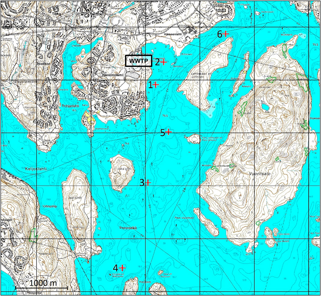
FIGURE 1. Study area. The depth of the sites was 5 m (sites one and 2), 12 m (site 3), 20 m (site 4), 24 m (site 5) and 14 m (site 6). The effluent waters of WWTP are released at site 1. Rapid Vaajakoski, the main source for through flow, is located north-east outside the figure.

2.2 Sediment sampling

BTCs were first determined in sediment samples cored with Limnos sediment sampler, which contained a series of rings and enabled the slicing of sediment layers at an exact thickness of 1 cm (Kansanen et al., 1991). The samples were collected from five sampling sites (Figure 1: sites 1, 2, 3, 5, 6) and three depths (0–1 cm, 1–3 cm, and 3–5 cm) to assess the presence of BTCs in old sediment layers. In the study area the sediment at the depth of 5 cm was about 10 years old (Paasivirta et al., 1990). If the settling velocity and the water quality have remained fairly similar, the samples taken at the depth of 2–3 cm could be estimated to be about 5 years old.

2.3 Grab water sampling

The concentrations of BTCs were monitored with grab water samples, which were taken every 2 weeks at the same time as the passive samplers and sedimentation traps were retrieved or emptied. The grab samples were collected in darkened glass bottles (1 L) from the depths of 1 m below the surface and 1 m above the lake bottom. At sites three to six, one grab sample was taken from the middle of the water column. Grab sampling was not conducted at site three in the second year due to financial limitations. The samples were stored at +4°C and were not filtered before analysis. The results are presented as an average of concentrations which exceeded the limit of detection (LOD). The LODs of this method were 0.50 ng L⁻¹ for MBT and DBT and 0.2 ng L⁻¹ for TBT (Supplementary Table S1).

2.4 Sedimentation traps

Sedimentation traps were deployed at each sampling site (1–6, Figure 1) to study the amount of settling particles and measure the particle-bound fraction of BTCs. Duplicate traps were placed 1 m above the lake bottom, where they collected settled particles for 2 weeks. After that, the samples were collected in glass jars and the traps were redeployed. The excess water was decanted and discarded, and the samples were stored at +4°C until analysis. BTCs were analyzed in the settled particles. The trap consisted of two acrylic tubes whose diameter (D) was 9.3 cm and height (H) was 50 cm, with the H/D ratio being 5.4. The top part of the tube was open, but the bottom was sealed to trap the particles. The ratio of the height and diameter (H/D) of the tube is essential to avoid the escaping of particles, with Bloesch and Burns (1980) recommending an H/D ratio of 5. According to Lau (1979), the critical stream velocity at 15°C for an H/D ratio of 6.7 was 26.2 cm s⁻¹ and for an H/D ratio of 10 it was 27 cm s⁻¹. In this study, the ratio was 5.4, so the escaping velocity was 26.2 cm s⁻¹. Such current velocities are extremely rare in Finnish lakes. In this study, the currents were also measured at the study site (Chapter 2.7). The results are expressed as dry weight (dw). The LODs of this method were 0.50 μg kg⁻¹ dw for MBT and DBT and 0.2 μg kg⁻¹ dw for TBT (Table S1).

2.5 Passive sampling

Three replicate Chemcatcher passive samplers with a C-18 Empore disk and polycarbonate housing (Ahkola et al., 2015, 2016) were deployed at each sampling site (1–6, Figure 1) for 2 weeks, after which they were retrieved and replaced with new ones. Samplers were deployed 1 m below the water’s surface. The samplers accumulated a dissolved fraction of the chemical which, after the deployment time period, was extracted from the sampler. TWA concentrations of dissolved BTCs during the 2-week sampling period were calculated using sampling rates determined in Ahkola et al. (2015, 2016). The method detection limit (MDL) was calculated from the analytical limit of detection (ng sampler⁻¹) after 14 days’ deployment and it was 0.016 ng L⁻¹ for MBT, 0.010 ng L⁻¹ for DBT and 0.0082 ng L⁻¹ for TBT (Supplementary Table S1).

2.6 Sample treatment and analysis

The Chemcatcher passive sampler contained a C-18 Empore disk as the receiving phase (47 mm diameter, 3 M Agilent Technologies Finland Oy) attached to polycarbonate sampler housing (AlControl AB, Linköping, Sweden) (Ahkola et al., 2015). After deployment, the internal standard (tri-n-propyltin) was added to the disk, which was further extracted with acetic acid–methanol (3:1) in an ultrasonic bath for 10 min. The sample was left to stand for 10 min and the ultra-sonication was repeated. A 4 ml acetate buffer (1 M, pH 5.4) was added and BTCs were derivatized with sodium tetraethylborate (NaB(C₂H₅)₄) and extracted from an acetic acid-methanol-acetic acid mixture to hexane, which was transferred to a sample vial and analyzed with GC-ICP-MS (Agilent 6890 N gas chromatograph coupled to Agilent 7500ce ICP-MS) (ISO 17353, 2004; Alonso et al., 2002; Ahkola et al., 2015). After the gas chromatographic separation of BTCs they were quantified according to Sn isotope concentrations using the internal standard technique. The determination method is accredited by the laboratory and QA/QC was conducted according to that. The results were expressed as a concentration of each BTC species. The sediment samples and settled particles from sedimentation traps were treated according to passive sampler procedure; the BTC concentrations are expressed as dw. The internal standard (tri-n-propyltin), acetate buffer (1 M, pH 5.4), and sodium tetraethylborate (NaB(C₂H₅)₄) were added to the grab water samples (V = 300 ml) and the BTCs were liquid-liquid extracted to hexane and analyzed with GC-ICP-MS. Before analysis, all the samples were stored at +4°C. The passive samplers, sediments, and settled particles were analyzed within 7 days of retrieval. The grab samples were analyzed the day after sampling. Blank samples were processed and measured alongside every sample treatment. The LOD for each sampling technique is presented in Supplementary Table S1. Concentrations of BTC in sedimented particles are expressed as average of two measurements in passive samplers as average of three replicates and those are used in calculating the annual average concentrations. One grab water sample was taken from two to three depths at each sampling site and the annual average concentrations are calculated from them.

2.7 Monitoring of water flow

The water flow was monitored with moored recording current meters (Aanderaa RCM-9) placed on sites 1, 2, and three to observe the water currents and to estimate the transportation of BTCs in the study area. The flow was measured at depths 1.1 m (site 1), 1.0 m (site 2), and 2.0 m (site 3) and currents were recorded as a 10-min average. Currents were measured for 3.5 months in both study years, covering the time of the monitoring campaigns.

2.8 Computational estimation of BTC sources

Computational simulation was conducted at the study area to estimate the transportation and distribution of BTCs in lake conditions. In computational transport modelling there are two fundamentally different approaches to consider dispersion of substances: Eulerian and Lagrangian. While in the Eulerian approach the concentration field is evaluated continuously for a whole modelled area, in the Lagrangian method the trajectory for each particle is modelled individually. This kind of modelling approach enables back tracking calculation in time as well as the estimation of the source of particles observed at the study area (Karjalainen et al., 2019).

To computationally estimate sources of BTCs and to create a flow model for the study area we used the COHERENS model V2.11.2 (Luyten 2013; COHERENS 2022). COHERENS is an ocean circulation model that solves Navier-Stokes equations using the Boussinesq approximation and the assumption of vertical hydrostatic equilibrium. The prime equations are solved in a horizontally uniform rectangular grid with the resolution of 100 m for both horizontal directions (84 and 115 grid cells in west-east and south-north directions, respectively) and with 10 terrain following σ-layers. Vertical mixing was based on k-ε turbulence scheme (k is turbulent energy and ε is rate of dissipation it), TVD (total variation diminishing) advection scheme was used for momentum and tracers and explicit horizontal diffusion was disabled. For turbulence quantities advection was disabled. The model runs were started from the rest, i.e., the initial values of 0 were used for currents and the temperature was adjusted to 5°C. The simulation periods were 1 May 2012–20 September 2012 and 1 May 2013–5 September 2013, covering the whole sampling period.

The Lagrangian particle module implemented in COHERENS uses currents to model the transportation of the individual particles. We used an approach where currents were calculated beforehand. Temporal resolution was 15 min. To consider the degradation path from TeBT to MBT, we modified the particle module of COHERENS to take into account this transformation chain and used the degradation rates presented in Juntunen et al. (2020). Different BTCs are represented as particles with differing properties. Same particle modules without a degradation chain have been used when estimating the reproducing strategies of larvae in surface waters (Karjalainen et al., 2019).

The modelled area was the north part of Lake Päijänne. The southern border was located in the middle of the lake and considered to be far enough, so the lack of actual flow data can be neglected. In the model we considered the Vaajakoski rapid in the north-east as an incoming boundary and that the discharge in the study area remained the same.

Two different situations were simulated with the model and the possible sources of BTCs were estimated. The constant presence of BTCs in the vicinity of the sampling sites was assumed. In the first simulation, one BTC particle for each species was released every minute during the 2-week passive sampler/sedimentation trap deployment period (20,160 particles/2 weeks). In the second simulation, 20,160 particles were released at once from the same locations as in the first case, which now mimicked the timing of instant grab water sampling. For both release types, either 20,160 particles in 2 weeks or 20,160 particles at once, the location of particles was back tracked to the beginning of the simulation period. Using back tracking calculation, the probability that particles were released from the WWTP (site 1) was assessed.

3 Results and discussion

To explain the transportation phenomena, it is important to understand the water currents prevailing in the study area. Knowledge concerning the currents also allows to estimate the probability of resuspension from sediments and hence the release of BTCs back to dissolved form. High flow velocity correlates rather well with the flow environment where instantaneous forces affect the suspended particulate matter and hence might release attached BTCs from the particles. Furthermore, measured velocities can be used to estimate the accuracy of the computational model applied in this paper.

3.1 Hydrological conditions and measured water currents

The study years were hydrologically very different. The average inflow to Lake Päijänne during the study period (May–September) was higher in the first year (264 m³ s⁻¹) than in the second (164 m³ s-¹) (Database for hydrological observations, SYKE). Also, the water levels during the study period differed, being 230 cm in first study year and 212 cm in the second. In addition, the runoff waters originated from watershed located upstream from the study area could have brought more pollutants to the study area.

When considering the flow velocity and current direction of the lake (Supplementary Table S2), the transportation of released effluent from site one downstream to site three lasted about 0.5 days. Site four was located twice as far away so the effluent reached it in 1 day. Though the current was not moving straightforwardly to the south but circulated, the results suggest that effluent can spread to the whole study area in approximately 2 days. The average water velocities during the 2-week sampling period varied, especially at site 3, where the highest velocities occurred during the time period of deployments five and 6 (in the first year) and deployments one and 2 (in the second year), being 5.8 cm s⁻¹ and 5.0 cm s⁻¹, respectively (Supplementary Table S2). However, the velocities were clearly below the limit value of 26.2 cm s⁻¹ so it is unlikely that the solid particles escaped from the trap. According to the measurements in Supplementary Table S2, the water currents may circulate the effluent waters upstream from site one to the upstream site two occasionally. This observation is also supported by the modeling results. The flow roses (Supplementary Figure S1) show that currents from site 1 toward site two were higher during the second study year than the first year. The hydrological differences between the study years can be observed at site three where varying flow direction mixed the water column during the second study year.

3.2 Sediment samples

The highest content of MBT, DBT, and TBT were found at site 1, which receives effluent waters including particles from the WWTP (Supplementary Figure S2; Supplementary Table S4). At site one the TBT content increased with the core depth (1.4 μg kg⁻¹, 54 μg kg⁻¹, and 64 μg kg⁻¹ from core depths 0–1 cm, 1–3 cm, and 3–5 cm, respectively), which suggests that the release of TBT has diminished in recent years. MBT and DBT concentrations decreased with the core depth, which suggests that they are still being released into the aquatic environment. According to simultaneous waste water study, OTCs were released from the WWTP since the effluent waters contained 0.2–2.0 ng L⁻¹ TBT, 1–18 ng L⁻¹ DBT, and 2.4–51 ng L⁻¹ MBT (Ahkola et al., 2016).

Sediment samples at sites 5 and 3, located at deep parts of the lake and downstream from the WWTP, had higher concentrations of BTCs than the reference site 6 (Supplementary Figure S2; Supplementary Table S4). This indicates that WWTP-originated particles drift mainly downstream and those sites can act as sedimentation sinks. Site six is in the main waterway and boat traffic may disturb the lake bottom, cause resuspension, and hinder the sedimentation process. Site two is in the shallow part of the lake away from the main waterway and, due to currents, receives some effluent from the WWTP.

In Lake Päijänne, BTCs have been previously measured in the surface sediment from the study area near sites one and between sites 3 and 4. The samples were taken at a depth of 2–3 cm and the contents of MBT, DBT, and TBT were 8.6 μg kg⁻¹, 1.8 μg kg⁻¹, and 0.9 μg kg⁻¹, respectively (Mannio et al., 2011). These results were somewhat lower than the ones observed in this study.

As there is no classification system for contaminated sediments in Finland, the concentrations can be compared with Norwegian and Swedish EQS values, which for TBT are 0.002 μg kg⁻¹ and 1.6 μg kg⁻¹, respectively (Olsen et al., 2019). The Norwegian EQS values were exceeded at all sampling sites but the Swedish EQS were exceeded only at site one at core depths 1–3 cm and 3–5 cm. This suggests that the sediment in the study area is contaminated by TBT.

3.3 Grab sampling

The concentration of BTCs in grab water samples was expected to be low and only concentrations which exceeded the LOD were included in the calculations. The MAC-EQS of TBT was exceeded only once, in a grab sample taken during the first study year. As the LOD of TBT was the same as AA-EQS, it was exceeded when observed. According to the literature, there are not many extant studies concerning the determination of BTCs in inland waters, possibly due to analytical restrictions deriving from the low concentrations. According to Aguilar-Martinez et al. (2011), the concentration of TBT in inland waters (Lake San Juan, Spain) remained below the LOD both in grab and passive sampling; the TBT LOD for grab samples was 9 ng L⁻¹, and for passive samplers 1.2 ng L⁻¹. MBT was detected in grab samples (4.0 ng L⁻¹) and passive samplers (9.1 ng L⁻¹) and DBT concentrations were (9.0 ng L⁻¹) and (2.6 ng L⁻¹), respectively. In Finland, BTCs have been studied in wastewater where MBT and DBT were detected in concentrations of 4–20 ng/L and 1.6–5.6 ng/L, respectively (Mannio et al., 2011). However, the TBT concentrations remained below the detection limit (0.5 ng/L). Also, Vieno (2014) measured TBT from 60 WWTP effluents and detected it in four samples with an average concentration of 0.22 ng/L. The MBT and DBT concentrations were considerably higher in the first year than in the second year (Figure 2, Supplementary Table S5, S6). In TBT concentrations this was observed as well but it was not that evident. All in all, the concentrations were mainly below the LOD throughout the sampling campaign in both years and were even lower in the second year.

FIGURE 2

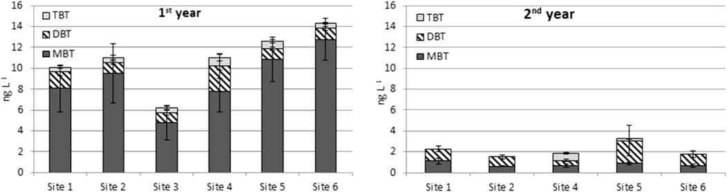
FIGURE 2. Average BTC concentrations in grab water samples.

3.4 Sedimentation traps

3.4.1 Settling particles in sedimentation traps

The highest amount of particles settled into sedimentation traps (as dw) was measured at site 1, which receives the effluent waters directly from the WWTP (Supplementary Figure S3). At reference site six the amounts of settling particles in the first study year were higher than at sites three to five, and twice as high than in the second year. This implies that particles drift upstream from the study area to site 6. In the second year the highest amount of settling particles was measured at site 2, which was located at the shallow part of the lake and had a lot of aquatic vegetation. Due to currents, site two also receives effluents from the WWTP, which can bring particles to the area. The amount of particles was the lowest at site 4, which is located furthest from the WWTP.

3.4.2 BTC concentrations in settling particles of sedimentation traps

The highest BTC concentrations (as dw) were measured at the outlet of the WWTP (site 1, Figure 3, Supplementary Table S7, S8). The high amount of settling particles found at sites two and six did not increase the BTC concentration (Supplementary Figures S3, S4). Thus, an apparent connection between the particle amount and the BTC concentration in settling particles was not observed. The BTC concentrations were slightly higher in the first year at all sites except for site 6. However, the differences are negligible. The relative abundance of MBT, DBT, and TBT at site one differed from the ones detected at the other sampling sites: at site one DBT dominated whereas MBT was the prevailing BTC at the rest of the sites (Figure 3). Notably, the high particle-bound BTC release from the WWTP in the first year could have been derived from a broken pipe which released activated sludge to the effluent and further to the watercourse. This accident is further discussed in Chapter 3.6.

FIGURE 3

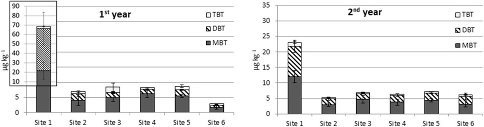
FIGURE 3. Average of MBT, DBT and TBT concentration in settling particles. Notice the scaling of the first years chart.

3.5 Passive sampling

The concentrations of BTCs observed with passive sampling were not clearly higher at the WWTP outflow (site 1) than at other sites (Figure 4; Supplementary Tables S9, S10). One reason for this is that the BTCs are bound to particles present in effluent waters and are not available for passive samplers. As with grab sampling data, higher BTC concentrations were detected in all Chemcatcher passive samplers deployed in the first year than those in the second year. However, the concentrations between these two sampling techniques are significant, as grab samples include both dissolved and particle-bound fractions. According to the results, the dissolved fraction of BTCs remained quite stable during both study years.

FIGURE 4

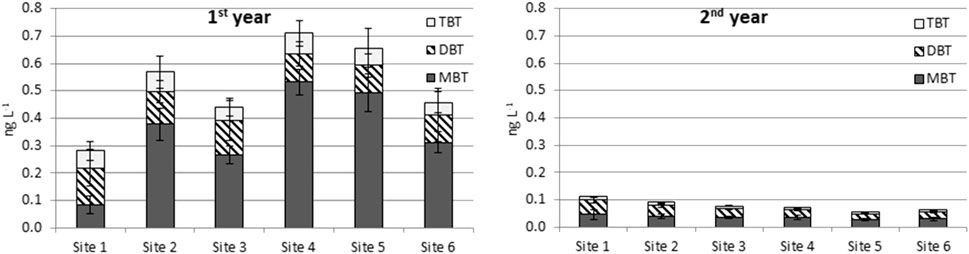
FIGURE 4. Average of MBT, DBT and TBT concentrations in Chemcatcher passive samplers.

3.6 Summary of the sampling techniques

The passive sampling technique had a lower LOD expressed as MDL over the 2-week deployment than grab sampling (Supplementary Table S1). MBT was detected in 29%–87% and DBT in 29%–55% of grab samples (Table 1). With passive sampling the detection percentage for MBT and DBT was 96%–100% and with sedimentation traps it was 67%–79%. However, TBT was detected only in 4%–24% of the grab samples, while detection with passive samplers was at 90%–94% and at 50%–52% with sedimentation traps. However, though the concentration of TBT in grab samples remained below the LOD (0.2 ng L⁻¹), it does not necessarily mean that TBT is not present in the aquatic environment. Passive samplers collect BTCs for a longer time period and if BTCs are present at even trace concentrations they will be enriched to the sampler so their concentrations can be measured. As TBT is detected more often in passive samplers than in grab samples, the samplers were able to detect the concentrations which in grab samples would remain undetected. This suggests that with passive sampling the presence of TBT in surface waters can be detected more reliably than with grab sampling.

TABLE 1

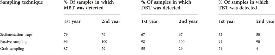
TABLE 1. Detection of BTCs with different sampling techniques.

The broken pipe at the WWTP released activated sludge with effluent waters to Lake Päijänne and site 1. The leak was noticed in the beginning of the first year’s sampling campaign on May 31st and was fixed on June 7th, so it took place during the first passive sampler and sedimentation trap deployment. The grab sampling was conducted 7 days after the leak (June 14th) and the leak was not noticed, with only slightly elevated MBT concentrations detected (Figure 5). A 2 weeks’ deployment of passive samplers during the leak (May 30th–June 14th) led to elevated concentrations of dissolved BTC and the concentrations decreased in the next sampling occasion. However, the concentrations increased again as the deployment trials continued. In settling particles data, the sludge release was discovered at high concentrations, which in the case of MBT and DBT diminished as the trials continued. As the BTCs were released with activated sludge, their detection in settling particles was more probable than with grab or passive samples.

FIGURE 5

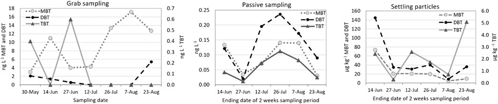
FIGURE 5. Concentration of BTCs at site one during the pipe broke at WWTP. Notice that the x-axis of passive samplers and sedimented particles describe the retrieval date after 2 weeks deployment but in grab sampling the exact sampling date.

3.7 Extreme value analysis

Determining BTCs from grab water samples requires analytical techniques with low quantification levels. Instant BTCs are seldom detected in Finnish surface waters by grab sampling, despite being present at trace concentrations. BTC concentrations tend to remain below the LOD of analysis method. Only the high peak concentrations of the underlying continuous time series are observed. This, however, does not mean that all observed values would be extreme values. In such cases traditional statistical analysis does not apply, i.e., statistical tests (such as the Student’s t-test) assuming normality fail. However, there is an own branch of statistics called “extreme value theory” which can be applied to study the behaviour and statistics of extreme values. More information about the extreme value analysis is presented in Supplementary data.

Threshold values u for concentrations, after which measurements are considered as extreme, are close to the LOD especially for TBT (Supplementary Tables S11–S13). The second study year’s threshold values for grab and passive samplers’ results are smaller than for the first study year. Generally, short-tailed distributions (ε > 0) are especially interesting, since they indicate a maximum possible value for observation. Based on shape parameters ε, presented in Supplementary Tables S11, S12, this is quite typical. For grab samples the distributions for MBT and TBT in the first year were short-tailed ones. From Supplementary Table S12 we can see that for MBT and DBT value ε > 0 in the first year while for TBT ε > 0 in the second year. Only for BTC measured from settled particles in sedimentation traps were systematically ε < 0 which means that many measurements are far from the central part of the distribution. Furthermore, different BTCs can be short- or long-tailed in the same year. When considering MBT from grab samples, the parameter describing the distributions of exceedances β deviates greatly between the first and second years (Supplementary Table S11). None of the values observed in the second year even exceeded the threshold of the first year. For DBT, the obtained values were much closer to each other, and for TBT, the number of observed values in the second year were so small that analysis was not reasonable.

For grab sampling, even long-tailed distribution (ε < 0) values were ε > -0.5, which means that the distributions have limited variance (Supplementary Table S11). For BTC determined from passive samplers or settled particles in sedimentation traps this does not apply anymore (Supplementary Tables S12, S13). One distribution for BTC gathered with sedimentation traps is so long-tailed that even the expected value u cannot be determined (Supplementary Table S13).

Considering the number of grab sampling observations that were higher than threshold value u, the MBT had the lowest percentage (51% in the first year and 56% in the second year) while DBT and first years’ TBT had percentages over 70% (Supplementary Table S11). This indicates that values of DBT and TBT are indeed extreme values. For passive sampling, the percentages of extreme values were significantly lower. This is expected, since passive sampling concentrates the low concentrations to a detectable level and the peak concentrations are integrated and seen as elevated TWA concentration. The extreme value percentages or MBT, were about 60%, for TBT about 37% while for DBT the percentages differed lot between the years being 44% and 81%. For BTC determined with sedimentation trap sampling the smallest percentage value was 69%.

The findings suggest that grab sampling and sedimentation trap sampling results contain more extreme peak values than passive sampling. Furthermore, deviation between threshold values u and LOD values indicates the applicability and usability of the sampling method. If the deviation is small, majority of observed values are extreme values and the mean or median of underlying concentration timeseries is very low, and vice versa. Extreme value analysis can therefore be used to estimate the actual level of the average concentration of BTC.

3.8 Computational estimation of sources of BTC

The computational modelling results imply that the effluent waters did not reach site six in conditions prevailing in the study area (Supplementary Figure S4). Positive values would indicate that the BTCs spread from site one upstream to site 6, but as the modelling results presented negative values (Supplementary Figure S4), it seems that the discharge spreads downstream. The grab water sampling and Chemcatcher passive sampling results suggest that site 6 has a rather high content of dissolved BTCs. In settled particles collected with sedimentation traps the BTC contents were low, which also implies that BTCs were in their dissolved form. However, the modelling reveals that these particles did not originate from the WWTP.

According to calculations, the BTCs detected at site one most apparently originated from the WWTP (Table 2). This is obvious, as site one receives the WWTP effluents. The next sites assumed to receive BTCs from the WWTP are 5, 2, and 3, but their order varied between the study years, possibly due to, for example, the prevailing currents (Supplementary Figure S1). The most unlikely sites to have particles originating from the WWTP are sites 4 and 6, which also supports the assumption that BTCs found at site six are from another source than the WWTP.

TABLE 2

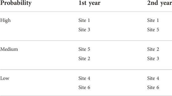
TABLE 2. The estimated probability class that the detected BTCs originate from WWTP.

The difference between the study years was also observed in the transportation simulations. The probability that BTC is discharged from WWTP and travels to location i (P_i) was systematically higher in the first study year than the second one. This appeared to be the case regardless of the simulation method used, whether mimicking passive sampling (continuous release of BTCs during the 2-week period) or grab sampling (same amount of BTCs released at once every 2 weeks). The simulation results show that it is nearly impossible that the observed BTCs would have come from the upstream site 6. When comparing the ratios of the most likely and most unlikely locations R_i = max (P_i)/min (P_i), we noticed deviation between the study years and an apparent difference between the simulation methods (Supplementary Table S3). It is expected that if the number of BTCs released during the 2-week time period (passive sampling) increases, the ratio of most likely and most unlikely locations would increase as well. However, the ratios R_i were systematically lower for the simulation mimicking passive sampling than the one mimicking grab sampling. This means that the most likely and most unlikely locations differ more when mimicking grab sampling release and suggests that the timing of instant grab sampling plays a more significant role in detecting pollutants, as expected.

4 Conclusion

The study years were hydrologically different, which was observed as higher dissolved BTC concentrations were determined with passive sampling during the first year. Still, their concentration in particle-bound fractions remained the same. In this study even the trace concentrations of BTCs were detected due to the enhanced sensitivity of the analyzing and sampling techniques. This enables a more accurate estimation of concentrations and to assess the condition of watercourses more precisely. As the AA-EQS of TBT was exceeded several times in grab water samples during the first study year, the lake does not seem to be in a good chemical condition. However, this assumption is not supported when considering the second study year, when only a few exceeding values were observed.

The extreme value analysis results reveal that grab sampling and sedimentation trap sampling results contain more extreme peak values than passive sampling. This suggests that the reliability of grab sampling is the lowest from the assessed techniques when the presence of BTCs is studied.

The assumption that BTCs are released only from the WWTP was not valid, as high concentrations were detected from sampling site six located upstream of the WWTP, which was considered a reference site for determining background concentration at the beginning of this study. Through computational modelling and back tracking simulations we were able to detect the possible sources of BTCs and found that they can come upstream of the sampling area where there are summer houses, boats, piers, and a wood processing industry presence. Hence, the WWTP cannot be considered as the only source of BTCs.

As the techniques enable to detect BTC concentrations near their EQS, they increase the reliability of the risk assessment. However, this also leads to the detection of pollutants at levels which may not have environmental effects. On the other hand, hydrophobic pollutants tend to accumulate in organisms and, due to the mixture effect, the awareness of these low concentrations may become essential. The trace concentrations can pose a risk if water is used, for example, for food production. Lake Päijänne provides raw water for drinking water production to the capital area and trace concentrations of harmful chemicals can pose a contamination.

There is no superior monitoring method for assessing the presence of organic chemicals in an aquatic environment with complicated properties. With grab sampling, BTC concentrations can remain below the detection limit, while integrative sampling methods, i.e., passive sampling and sedimentation traps, measure chemicals from different matrices. Hence, they should be employed as complementary methods when studying BTCs.

Data availability statement

The original contributions presented in the study are included in the article/Supplementary Material, further inquiries can be directed to the corresponding author.

Author contributions

HA, Responsible for organizing funding, planning the field trials, compiling, and processing the BTC results and writing and editing the manuscript. JJ, Responsible for planning and conducting the field trials, computational estimations, extreme value analysis and writing and editing the manuscript. KK, Responsible for organizing funding, planning and conducting the field trials and editing the manuscript. TH, Responsible for organizing funding, planning the field trials and editing the manuscript.

Funding

This study was supported by European Regional Development Fund, Maj and Tor Nessling foundation and Maa-ja vesitekniikan tuki ry.

Acknowledgments

The help of M. Sc. Petri Nieminen and M. Sc. Tino Hovinen for conducting the passive sampling trials is greatly appreciated. The effort of B.Sc. Saara Haapala, M. Sc. Tiina Virtanen, Rauni Kauppinen, Samuli Pietiläinen and Aleksi Tiusanen on the sample treatment is highly appreciated.

Conflict of interest

The authors declare that the research was conducted in the absence of any commercial or financial relationships that could be construed as a potential conflict of interest.

Publisher’s note

All claims expressed in this article are solely those of the authors and do not necessarily represent those of their affiliated organizations, or those of the publisher, the editors and the reviewers. Any product that may be evaluated in this article, or claim that may be made by its manufacturer, is not guaranteed or endorsed by the publisher.

Supplementary material

The Supplementary Material for this article can be found online at: https://www.frontiersin.org/articles/10.3389/fenvc.2022.1063667/full#supplementary-material

References

Aguilar-Martinez, R., Gomez-Gomez, M. M., and Palacios-Corvillo, M. A. (2011). Mercury and organotin compounds monitoring in fresh and marine waters across Europe by Chemcatcher passive sampler. Int. J. Environ. Anal. Chem. 91 (11), 1100–1116. doi:10.1080/03067310903199534

CrossRef Full Text | Google Scholar

Aguilar-Martinez, R., Greenwood, R., Mills, G. A., Vrana, B., Palacios-Corvillo, M. A., and Gomez-Gomez, M. M. (2008a). Assessment of Chemcatcher passive sampler for the monitoring of inorganic mercury and organotin compounds in water. Int. J. Environ. Anal. Chem. 88 (2), 75–90. doi:10.1080/03067310701461870

CrossRef Full Text | Google Scholar

Aguilar-Martinez, R., Palacios-Corvillo, M. A., Greenwood, R., Mills, G. A., Vrana, B., and Gomez-Gomez, M. M. (2008b). Calibration and use of the Chemcatcher® passive sampler for monitoring organotin compounds in water. Anal. Chim. Acta 618 (2), 157–167. doi:10.1016/j.aca.2008.04.052

PubMed Abstract | CrossRef Full Text | Google Scholar

Ahkola, H., Herve, S., and Knuutinen, J. (2013). Overview of passive Chemcatcher sampling with SPE pretreatment suitable for the analysis of NPEOs and NPs. Environ. Sci. Pollut. Res. 20 (3), 1207–1218. doi:10.1007/s11356-012-1153-0

PubMed Abstract | CrossRef Full Text | Google Scholar

Ahkola, H., Herve, S., and Knuutinen, J. (2014). Study of different Chemcatcher configurations in the monitoring of nonylphenol ethoxylates and nonylphenol in aquatic environment. Environ. Sci. Pollut. Res. 21 (15), 9182–9192. doi:10.1007/s11356-014-2828-5

PubMed Abstract | CrossRef Full Text | Google Scholar

Ahkola, H., Juntunen, J., Krogerus, K., Huttula, T., Herve, S., and Witick, A. (2016). Suitability of Chemcatcher® passive sampling in monitoring organotin compounds at a wastewater treatment plant. Environ. Sci. Water Res. Technol. 2 (4), 769–778. doi:10.1039/c6ew00057f

CrossRef Full Text | Google Scholar

Ahkola, H., Juntunen, J., Laitinen, M., Krogerus, K., Huttula, T., Herve, S., et al. (2015). Effect of the orientation and fluid flow on the accumulation of organotin compounds to Chemcatcher passive samplers. Environ. Sci. Process. Impacts 17 (4), 813–824. doi:10.1039/c4em00585f

PubMed Abstract | CrossRef Full Text | Google Scholar

Allan, I. J., Knutsson, J., Guigues, N., Mills, G. A., Fouillac, A. M., and Greenwood, R. (2007). Evaluation of the Chemcatcher and DGT passive samplers for monitoring metals with highly fluctuating water concentrations. J. Environ. Monit. 9 (7), 672–681. doi:10.1039/b701616f

PubMed Abstract | CrossRef Full Text | Google Scholar

Alonso, J. I. G., Encinar, J. R., Gonzalez, P. R., and Sanz-Medel, A. (2002). Determination of butyltin compounds in environmental samples by isotope-dilution GC-ICP-MS. Anal. Bioanal. Chem. 373 (6), 432–440. doi:10.1007/s00216-002-1294-y

PubMed Abstract | CrossRef Full Text | Google Scholar

Berto, D., Giani, M., Boscolo, R., Covelli, S., Giovanardi, O., Massironi, M., et al. (2007). Organotins (TBT and DBT) in water, sediments, and gastropods of the southern Venice lagoon (Italy). Mar. Pollut. Bull. 55 (10-12), 425–435. doi:10.1016/j.marpolbul.2007.09.005

PubMed Abstract | CrossRef Full Text | Google Scholar

Bloesch, J., and Burns, N. M. (1980). A critical-review of sedimentation trap technique. Schweiz. z. Hydrol. 42 (1), 15–55. doi:10.1007/bf02502505

CrossRef Full Text | Google Scholar

Blom, L. B., Morrison, G. M., Kingston, J., Mills, G. A., Greenwood, R., Pettersson, T. J. R., et al. (2002). Performance of an in situ passive sampling system for metals in stormwater. J. Environ. Monit. 4 (2), 258–262. doi:10.1039/b200135g

PubMed Abstract | CrossRef Full Text | Google Scholar

Bryan, G. W., and Gibbs, P. E. (1991). “Impact of low concentrations of tributyltin (TBT) on marine organisms: A review,” in Metal ecotoxicology, concepts and applications. Editors M. C. Newman, and A. W. McIntosh. 1st ed. (Chelsea: Lewis Publishers).

Google Scholar

M. A. Champ, and P. F. Seligman (Editors) (1996). Organotin - environmental fate and effects. 1st ed. (London: Chapman & Hall).

Google Scholar

COHERENS (2022). COHERENS, modelling system for shallow waters, current version: v.2.11.2, RBINS 2014–2022 » operational directorate natural environment. Available at https://odnature.naturalsciences.be/coherens/(Accessed 11 10, 2022).

Google Scholar

Cole, R. F., Mills, G. A., Hale, M. S., Parker, R., Bolam, T., Teasdale, P. R., et al. (2018). Development and evaluation of a new diffusive gradients in thin-films technique for measuring organotin compounds in coastal sediment pore water. Talanta 178, 670–678. doi:10.1016/j.talanta.2017.09.081

PubMed Abstract | CrossRef Full Text | Google Scholar

de la Cal, A., Kuster, M., de Alda, M. L., Eljarrat, E., and Barcelo, D. (2008). Evaluation of the aquatic passive sampler Chemcatcher for the monitoring of highly hydrophobic compounds in water. Talanta 76 (2), 327–332. doi:10.1016/j.talanta.2008.02.049

PubMed Abstract | CrossRef Full Text | Google Scholar

Dı́ez, S., Abalos, M., and Bayona, J. M. (2002). Organotin contamination in sediments from the Western Mediterranean enclosures following 10 years of TBT regulation. Water Res. 36 (4), 905–918. doi:10.1016/s0043-1354(01)00305-0

PubMed Abstract | CrossRef Full Text | Google Scholar

Dowson, P. H., Bubb, J. M., and Lester, J. N. (1993). A study of the partitioning and sorptive behaviour of butyltins in the aquatic environment. Appl. Organomet. Chem. 7 (8), 623–633. doi:10.1002/aoc.590070805

CrossRef Full Text | Google Scholar

Dubalska, K., Rutkowska, M., Bajger-Nowak, G., Konieczka, P., and Namiesnik, J. (2013). Organotin compounds: Environmental fate and analytics. Crit. Rev. Anal. Chem. 43 (1), 35–54. doi:10.1080/10408347.2012.743846

CrossRef Full Text | Google Scholar

European Council (2008). Directive 2008/105/EC of the European Parliament and the Council of 16 December 2008 on environmental quality standards in the field of water policy. Official J. Eur. Union 348, 84–97.

Google Scholar

Fent, K. (1996). Organotin compounds in municipal wastewater and sewage sludge: Contamination, fate in treatment process and ecotoxicological consequences. Sci. Total Environ. 185 (1-3), 151–159. doi:10.1016/0048-9697(95)05048-5

CrossRef Full Text | Google Scholar

Filipkowska, A., Kowalewska, G., and Pavoni, B. (2014). Organotin compounds in surface sediments of the southern baltic coastal zone: A study on the main factors for their accumulation and degradation. Environ. Sci. Pollut. Res. 21 (3), 2077–2087. doi:10.1007/s11356-013-2115-x

PubMed Abstract | CrossRef Full Text | Google Scholar

Garnier, A., Bancon-Montigny, C., Delpoux, S., Spinelli, S., Avezac, M., and Gonzalez, C. (2020). Study of passive sampler calibration (Chemcatcher®) for environmental monitoring of organotin compounds: Matrix effect, concentration levels and laboratory vs in situ calibration. Talanta 219, 121316.

PubMed Abstract | CrossRef Full Text | Google Scholar

Górecki, T., and Namieśnik, J. (2002). Passive sampling. Trac-Trend Anal. Chem. 21 (4), 276–291.

Google Scholar

Gunold, R., Schafer, R. B., Paschke, A., Schuurmann, G., and Liess, M. (2008). Calibration of the Chemcatcher® passive sampler for monitoring selected polar and semi-polar pesticides in surface water. Environ. Pollut. 155 (1), 52–60. doi:10.1016/j.envpol.2007.10.037

PubMed Abstract | CrossRef Full Text | Google Scholar

Harino, H., Fukushima, M., Yamamoto, Y., Kawai, S., and Miyazaki, N. (1998). Organotin compounds in water, sediment, and biological samples from the Port of Osaka, Japan. Archives Environ. Contam. Toxicol. 35 (4), 558–564. doi:10.1007/s002449900416

PubMed Abstract | CrossRef Full Text | Google Scholar

Hoch, M. (2001). Organotin compounds in the environment - an overview. Appl. Geochem. 16 (7-8), 719–743. doi:10.1016/s0883-2927(00)00067-6

CrossRef Full Text | Google Scholar

ISO 17353 (2004). Water quality: Determination of selected organotin compounds: Gas chromatographic method. Geneva, Switzerland: International Organization for Standardization.

Google Scholar

Juntunen, J., Ahkola, H., Krogerus, K., and Huttula, T. (2020). New theory of time integrative passive samplers. Anal. Chim. Acta 1127, 269–281. doi:10.1016/j.aca.2020.05.042

PubMed Abstract | CrossRef Full Text | Google Scholar

Kaitaranta, J., Niemisto, J., Buhvestova, O., and Nurminen, L. (2013). Quantifying sediment resuspension and internal phosphorus loading in shallow near-shore areas in the Gulf of Finland. Boreal Environ. Res. 18 (6), 473–487.

Google Scholar

Kansanen, P. H., Jaakkola, T., Kulmala, S., and Suutarinen, R. (1991). Sedimentation and distribution of gamma-emitting radionuclides in bottom sediments of southern Lake Paijanne, Finland, after the Chernobyl accident. Hydrobiologia 222 (2), 121–140. doi:10.1007/bf00006100

CrossRef Full Text | Google Scholar

Karjalainen, J., Juntunen, J., Keskinen, T., Koljonen, S., Nyholm, K., Ropponen, J., et al. (2019). Dispersion of vendace eggs and larvae around potential nursery areas reveals their reproductive strategy. Freshw. Biol. 64 (5), 843–855. doi:10.1111/fwb.13267

CrossRef Full Text | Google Scholar

Kingston, J. K., Greenwood, R., Mills, G. A., Morrison, G. M., and Persson, L. B. (2000). Development of a novel passive sampling system for the time-averaged measurement of a range of organic pollutants in aquatic environments. J. Environ. Monit. 2 (5), 487–495. doi:10.1039/b003532g

PubMed Abstract | CrossRef Full Text | Google Scholar

Kot, A., Zabiegala, B., and Namiesnik, J. (2000). Passive sampling for long-term monitoring of organic pollutants in water. TrAC Trends Anal. Chem. 19 (7), 446–459. doi:10.1016/s0165-9936(99)00223-x

CrossRef Full Text | Google Scholar

Lau, Y. L. (1979). Laboratory study of cylindrical sedimentation traps. J. Fish. Res. Bd. Can. 36, 1288–1291. doi:10.1139/f79-184

CrossRef Full Text | Google Scholar

Lindholm-Lehto, P. C., Ahkola, H. S. J., and Knuutinen, J. S. (2018). Pharmaceuticals in processing of municipal sewage sludge studied by grab and passive sampling. Water Qual. Res. J. 53 (1), 14–23. doi:10.2166/wqrj.2018.022

CrossRef Full Text | Google Scholar

Luyten, P. (2013). COHERENS—a coupled hydrodynamical-ecological model for regional and shelf seas: User documentation. Version 2.5.1. RBINS-MUMM report, royal Belgian Institute of natural sciences. Available at http://odnature.naturalsciences.be/coherens/.

Google Scholar

Mannio, J., Mehtonen, J., Londesborough, S., Grönroos, M., Paloheimo, A., Köngäs, P., et al. (2011). Screening of hazardous industrial and household chemicals in the aquatic environment. Finn. Environ. 3.

Google Scholar

Olsen, M., Petersen, K., Lehoux, A. P., Leppänen, M., Schaanning, M., Snowball, I., et al. (2019). Contaminated sediments: Review of solutions for protecting aquatic environments. Nordic Counc. Minist. TemaNord 2019, 514. doi:10.6027/TN2019-514

CrossRef Full Text | Google Scholar

Paasivirta, J., Särkkä, J., Maatela, P., Welling, L., Paukku, R., Hakala, H., et al. (1990). Organoklooriyhdisteiden kulkeutumistutkimus Keski-Suomen järvisedimenteistä. Vesi- ja ympäristöhallituksen Monistesar. 280, 1–58.

Google Scholar

Page, D. S., Ozbal, C. C., and Lanphear, M. E. (1996). Concentration of butyltin species in sediments associated with shipyard activity. Environ. Pollut. 91 (2), 237–243. doi:10.1016/0269-7491(95)00046-1

PubMed Abstract | CrossRef Full Text | Google Scholar

Persson, L. B., Morrison, G. M., Friemann, J. U., Kingston, J., Mills, G., and Greenwood, R. (2001). Diffusional behaviour of metals in a passive sampling system for monitoring aquatic pollution. J. Environ. Monit. 3 (6), 639–645. doi:10.1039/b107959j

PubMed Abstract | CrossRef Full Text | Google Scholar

Sánchez-Bayo, F., Hyne, R. V., Kibria, G., and Doble, P. (2013). Calibration and field application of chemcatcher(A (R)) passive samplers for detecting amitrole residues in agricultural drain waters. B. Environ. Contam. Tox. 90 (6), 635–639.

Google Scholar

Schubert, B., Heininger, P., Keller, M., Ricking, M., and Claus, E. (2012). Monitoring of contaminants in suspended particulate matter as an alternative to sediments. TrAC Trends Anal. Chem. 36, 58–70. doi:10.1016/j.trac.2012.04.003

CrossRef Full Text | Google Scholar

Seligman, P. F., Valkirs, A. O., and Lee, R. F. (1986). Degradation of tributyltin in san-diego bay, California, waters. Environ. Sci. Technol. 20 (12), 1229–1235. doi:10.1021/es00154a006

CrossRef Full Text | Google Scholar

Vermeirssen, E. L. M., Dietschweiler, C., Escher, B. I., van der Voet, J., and Hollender, J. (2013). Uptake and release kinetics of 22 polar organic chemicals in the Chemcatcher passive sampler. Anal. Bioanal. Chem. 405 (15), 5225–5236. doi:10.1007/s00216-013-6878-1

PubMed Abstract | CrossRef Full Text | Google Scholar

Vieno, N. (2014). “Hazardous substances at wastewater treatment project report, Vesilaitosyhdistyksen monistesarja nro 34, Finnish Water Utilities Association,” in Finnish.

Google Scholar

Vrana, B., Mills, G. A., Allan, I. J., Dominiak, E., Svensson, K., Knutsson, J., et al. (2005b). Passive sampling techniques for monitoring pollutants in water. TrAC Trends Anal. Chem. 24 (10), 845–868. doi:10.1016/j.trac.2005.06.006

CrossRef Full Text | Google Scholar

Vrana, B., Mills, G. A., Dominiak, E., and Greenwood, R. (2006). Calibration of the Chemcatcher passive sampler for the monitoring of priority organic pollutants in water. Environ. Pollut. 142 (2), 333–343. doi:10.1016/j.envpol.2005.10.033

PubMed Abstract | CrossRef Full Text | Google Scholar

Vrana, B., Mills, G., Greenwood, R., Knutsson, J., Svenssone, K., and Morrison, G. (2005a). Performance optimisation of a passive sampler for monitoring hydrophobic organic pollutants in water. J. Environ. Monit. 7 (6), 612–620. doi:10.1039/b419070j

PubMed Abstract | CrossRef Full Text | Google Scholar

Vrana, B., Vermeirssen, E. L. M., Allan, I. J., Kohoutek, J., Kennedy, K., Mills, G. A., et al. (2009). “Passive sampling of emerging pollutants in the aquatic environment: State of the art and perspectives,” in Position Paper. NORMAN—network of reference laboratories, research centre and related organisations for monitoring of emerging environmental substances.

Google Scholar

Wren, D. G., Taylor, J. M., Rigby, J. R., Locke, M. A., and Yasarer, L. M. W. (2019). Short term sediment accumulation rates reveal seasonal time lags between sediment delivery and deposition in an oxbow lake. Agric. Ecosyst. Environ. 281, 92–99. doi:10.1016/j.agee.2019.05.007

CrossRef Full Text | Google Scholar