Dynamic and Interpretable Hazard-Based Models of Traffic Incident Durations

1 Introduction

Managing and reducing congestion on roads is a fundamental challenge faced across the world. In many countries, one being the United Kingdom, there is limited scope to build additional infrastructure to cope with the demand for road traffic. Instead, the focus is on an approach referred to as “Intelligent Mobility”, broadly described as combining real-time data and modeling to improve the management of existing physical infrastructure. An appropriate test-bed for such approaches is the United Kingdom Strategic Road Network (SRN), which constitutes around 4,400 miles of motorways and major trunk roads across England (see Peluffo, 2015). Further, the SRN carries 30% of all traffic in the United Kingdom, with 4 million vehicles using it everyday and 1 billion tonnes of freight being transported across it each year (see Highways England, 2017). There is little chance that in the short term, the SRN will see significant infrastructure changes, however data describing the traffic state across the network is already being collected and made available for analysis. While a significant component of the United Kingdom transport infrastructure, congestion remains a major problem on the network, with the cited report suggesting 75% of businesses consider tackling congestion on the SRN is important or critical to their business.

Traffic congestion can be broadly separated into two types: recurrent and non-recurrent. Recurrent congestion is simply the result of the demand regularly exceeding capacity on busy sections of road during “rush hour” periods. Non-recurrent congestion on the other hand is mainly caused by traffic incidents and rare incidents (Li et al., 2018). To better manage traffic during these incidents, traffic operators require reliable estimates of how long a particular incident will last. While there is significant existing work on modeling incident duration, many fundamental challenges remain that are both of practical interest to traffic management centers and remain active areas of research in an academic sense. A review of existing work on this problem is found in Li et al. (2018), where six future challenges for incident duration prediction are listed. These are: combining multiple data-sources, time sequential prediction models, outlier prediction, improvement of prediction methods through machine learning or alternative frameworks, combining recovery times and accounting for unobserved factors. Our work aims to address five of these challenges, combining time-series from sensor networks with incident reports to issue dynamically updated duration predictions. Inspired by approaches adopted in medical applications, we consider classical survival approaches and non-linear, machine learning methods for prediction, understanding where gains in performance are attained. Finally, as we are able to observe traffic behavior over long periods of time through the sensor network, we are able to judge not just when a traffic incident has been cleared, but when the traffic state has returned to normal operating conditions, thereby combining recovery times into our modeling approach.

The rest of this paper is structured as follows. Firstly, we overview existing work on incident duration prediction, specifying how the duration is defined, existing methods and offer more detail on challenges highlighted in the literature. Secondly, we detail our dataset, its collection and processing and an initial exploratory analysis of it. We then describe the considered modeling approaches, both for static and dynamic predictions, and results for our dataset. Finally, we consider what variables are important for the models and end by summarizing our main findings.

Note that throughout this paper, an “event” is defined as the traffic state on a section of road returning to a baseline behavior. As such, when an event has “occurred” we really mean the traffic state has recovered. This is just a note of terminology commonly used in the survival analysis literature.

2 Background

In this section, we summarize existing work on traffic incident duration analysis that is relevant to our own, along with relevant research from other disciplines that has influenced our approach.

Before any methodologies are considered, it is first important to define exactly what is being modeled. A traffic incident is considered to have four different time-phases: the time taken to detect and report an incident, the time to dispatch an operator to the scene, the travel time of the operator to the scene, and finally the time to clear an incident. Such a framework is described in Li et al. (2018). We consider an incident to have “started” when the incident is reported by the human operator, who would use a series of cameras to observe the state of the road in the case of the SRN. Our focus is to model the time from this point until both the incident has been physically cleared, and traffic behavior on the road has returned to some sense of “normal” behavior. We describe exactly how we determine normal behavior in section 3. In brief, we use a seasonal model of the speed time-series to estimate when the traffic speed on a section of road has recovered to a level close to what would be normally be expected for that section at that time of day. The idea to use such a speed profile is also considered in Hojati et al. (2014), where they define the “total incident duration” to be the time from incident start until the speed has recovered to the profile.

Whatever explicit definition of duration is used, there is an enormous amount of work on predicting incident durations. An initial step of many of these is to determine an appropriate distributional form that the durations take. These are typically heavy tailed and empirically show significant variation. Examples of this include modeling the distribution of incident durations as log-normal in Golob et al. (1987) and Chung and Yoon (2012), log-logistic in Zhang and Khattak (2010) and Junhua et al. (2013), Weibull in Hojati et al. (2014) and Al Kaabi et al. (2012), and generalized F in Ghosh et al. (2014). In the latter, it is noted that the generalized F distribution can be equivalent to many other distributional forms for particular parameter choices, including the exponential, Weibull, log-normal, log-logistic and gamma distributions. Hence, it offers more freedom than choosing any single one of these forms. Indeed, the authors state that the increased flexibility it offers allows it to fit the data better. Even further flexibility in the distributional choice is given in Zou et al. (2016), where it was shown that modeling the distribution as a mixture, that is the sum of multiple components, may improve model performance. Specifically, they consider a 2-component log-logistic mixture model, where the final distribution is the weighted average of two log-logistic distributions. Finally, other authors Smith and Smith (2001) have had difficulty finding statistically defensible distributional fits to their data, although it should be noted that different definitions of incident durations will likely impact this.

Using common probability distribution is appealing as it limits a model’s freedom and can be easier to fit to data. However, it is clear that authors are exploring more complex distributional forms to better model the data and seeing better results when they do so, as in Ghosh et al. (2014) and Zou et al. (2016). Mixture distributions are a naturally appealing form, as we assume the data is generated by multiple sub-populations, and can have different effects of covariates for different populations. We incorporate ideas from this section of the literature by considering models that assume log-normal and Weibull distributions on incident durations, as-well as mixture distributions where one supposes the data is generated by one of many sub-populations, each of which has a parametric form. Recent applications of survival analysis in healthcare Lee et al. (2018) have removed distributional assumptions entirely, and instead formulate models that output distributions with no closed form. This is done by treating the output space as discrete, and treating the model output as a probability mass function (PMF) defined over it, allowing for construction of a fully non-parametric estimate. Such an approach offers even more freedom, and as we see more complex distributions used in the traffic literature to provide more freedom, one could ask if removing the distribution assumption entirely can improve model performance.

After a distribution is determined, many works focus on methods from survival analysis, with a common choice being the Accelerated Failure Time (AFT) model. Example applications of this are given in Nam and Mannering (2000), Chung et al. (2010) and Chung et al. (2015). Such a model assumes that each covariate either accelerates or decelerates the life-time of a particular individual. These models are widely used, and offer an interpretable means of investigating what factors strongly or weakly influence incident duration. However, it can be difficult to incorporate time-series features into them. While it is possible to model time-varying effects of covariates, for example in Zeng and Lin (2007), it is more complex to derive optimal features from a time-series that are also interpretable. Clearly, AFT models are useful in that they produce interpretable outputs and relationships between variables, and can model the non-Gaussian distributions empirically observed in incident duration data. The alternative and well known classical survival model one could apply is a Cox regression model Cox (1972). Such a model assumes a baseline hazard function for the population, describing the instantaneous rate of incidents, from which survival probabilities can be calculated, see section 4.2 for more details. Covariate vectors for individuals shift this baseline hazard allowing for individualized predictions. Applications of this to transportation problems are given in Oralhan and Göktolga (2018), Wu et al. (2013) and Li and Guo (2014).

While these two methods are widely used, a number of alternatives exist. One such method is a sequential regression approach, an early example being Khattak et al. (1995). Importantly, the authors identify that more information describing an incident will become available over time, and hence consider a series of models to make sequential predictions. However, their sequential information was more descriptive from an operational stand-point, for example identifying damage to the road and response time of rescue vehicles. We do not have this, and instead focus on the minute-to-minute updates provided through traffic time-series recorded by sensors along the road, and how to engineer features from these. Truncated regression approaches were discussed in Zhang and Khattak (2010), where there was a specific effort to model “cascading” incidents (referred to as primary and secondary incidents in some literature). The thought here was that incidents that occur nearby in time and space would lead to a significantly longer clearance time for the road segment, and hence this should be accounted for in modeling. We performed an extensive analysis of primary and secondary incidents in our dataset in Kalair et al. (2021). Building on this and the previous cited work, we include a cascade variable in the models, allowing this to influence duration predictions.

Further regression approaches are explored in Garib et al. (1997) and Weng et al. (2015), and switching regression models are used in Ding et al. (2015). Note that in Weng et al. (2015), the authors first cluster the incident data, then use this clustering as additional features for a model, further suggesting that there is some element of sub-population structure in the data. A final relevant regression based work is Khattak et al. (2016), where quantile regression is used to model incident durations. This is a natural choice, as there is a clear skew in the empirically observed duration distributions, and if one does not want to assume a particular distributional form, they can instead model properties of the distribution, in this case quantiles of the data.

Further methodologies to note are those based on tree models or ensembles of them, particularly because we apply such a method later in this work. Tree based models are discussed in Smith and Smith (2001), where the authors compare models that assume particular incident duration distributions, a k-nearest-neighbour approach and a classification tree method based on predicting “short”, “medium” and “long” incidents. They concluded that no model provided accurate enough results on their dataset to warrant industrial implementation, but found the classification tree was the preferred model of those considered. Further, Zhan et al. (2011) considered a regression tree approach, where the terminal nodes of each tree were themselves multivariate linear models. Such an approach avoids binning of incidents into pre-defined categories, and achieved 42.70% mean absolute percentage error, better than the compared reference models. From an interdisciplinary setting, alternative tree methods have been considered, namely one known as “random survival forests” Ishwaran et al. (2008) as an extension to random forests to a survival analysis setting. In such a framework, the terminal nodes of each tree specify cumulative hazard functions for all data-points that fall into that node, and these hazards are combined across many trees to determine an ensemble hazard. There is no defined distributional assumption in such a model, again leaning toward the side of freedom in allowing the data to construct its own hazard function estimate rather than parametrizing an estimated form.

Neural networks are a rapidly developing methodology in machine learning, and have been used extensively in incident duration prediction and form the basis for some of our considered approaches. Examples of this include Wang et al. (2005), Wei and Lee (2005) and Lee and Wei (2010). Each of these applies feed forward neural networks to determine estimates of incident durations, and particularly in Lee and Wei (2010) sequential prediction was considered, using two models. The first took standard inputs, and the second took these along with detector information near the incident. These were input into feed-forward neural networks, and used to generate point predictions. Additional neural network applications are given in Valenti et al. (2010), where their performance is compared to that of linear regressions, decision trees, support vector machines and k-nearest-neighbour methods. The authors find that different models have optimal performance at different incident durations, suggesting there is still much to improve on feed forward networks. A final point to note is that neural networks have been applied to survival analysis problems in healthcare a number of times. Examples of this include Katzman et al. (2018) which develops a Cox model, replacing linear regression with a neural network output, Lee et al. (2018) which removes any distributional assumptions, and Jarrett et al. (2020) which uses a sliding window mechanism and temporal convolutions for dynamic predictions. We consider if the later two are useful in the application to traffic incidents later in this work. Specifically, using Jarrett et al. (2020) offers an automated way to engineer features from our sensor network data, while being able to model a parametric or non-parametric output.

While we have discussed a number of different methodological approaches, the actual features used to make these predictions, regardless of approach, appear quite consistent across different works. In Garib et al. (1997), the authors state that using number of lanes affected, number of vehicles involved, truck involvement, time of day, police response time and weather condition, one can explain 81% of variation in incident duration. An overview of various feature types is given in Li et al. (2018), identifying incident characteristics, environmental conditions, temporal characteristics, road characteristics, traffic flow measurements, operator reactions and vehicle characteristics as important factors when modeling incident durations.

We note that we are not the first to use sensor data in incident duration analysis. Speed data collected from roads was used in Ghosh et al. (2014), where the authors included two features based on the speed series: if the difference between the 15th and 85th percentiles of the speed data was greater than 7 mph and if the 85th percentile for speed was less than 70mph. Further, in Wei and Lee (2007) and Lee and Wei (2010) the authors train two feed forward neural networks, with input features that include the speed and flow for detectors near the incident. The first model provided a forecast just before the incident occurred, where as new data was fed into the second whenever available, updating predictions as time progressed. In the second paper, the focus was on reducing the dimensionality of the problem through feature selection via a genetic algorithm. We fundamentally differ from these for multiple reasons. With regard to Ghosh et al. (2014), this was an analysis of which factors impact incident duration the most, and where as they used hazard based models for analysis, we use the sensor data to engineer dynamic features, either manually or through temporal convolutions. Additionally, we differ from Wei and Lee (2007) and Lee and Wei (2010) through how we determine features and network structure, and through predicting an output distribution, not just a point estimate.

With dynamic prediction being highlighted as an area to address in the literature, some recent papers have looked at this problem through different methods to those already discussed. One example of this is Li et al. (2015), where a topic model was used to interpret written report messages and predictions were made as new textual information arrived. Further, multiple regression models were built in Ghosh et al. (2019), and as different features became available, data-points were assigned clusters, and a prediction was generated using a regression model tailored to each cluster. Lastly Li et al. (2020) considered a five stage approach, where a prediction was made at each stage and different features were available defining these stages. These included vehicles involved, agency response time and number of agencies responding. While this structured approach addresses some aspects of dynamic prediction, the purely data-driven approach which we present in this paper provides much more flexibility.

3 Data Collection and Processing

As discussed, various traffic data for the SRN is provided by a system called the National Traffic Information Service (NTIS)¹. This is both historic and real-time data. While the SRN includes all motorways and major A-roads in the United Kingdom, we focus our analysis on one the busiest United Kingdom motorways, the M25 London Orbital, pictured in Figure 1. Inside NTIS, roads are represented by a directed graph, with edges (referred to as links from now on) being segments of road that have a constant number of lanes and no slip roads joining or leaving. We extract all links that lie on the M25 in the clockwise direction, yielding a subset of the road network to collect data for. Placed along links are physical sensors called “loops”, which record passing vehicles and report averaged quantities each minute.

FIGURE 1

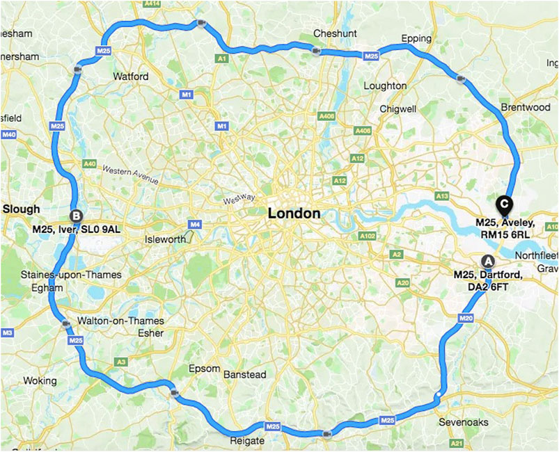
FIGURE 1. The M25 London Orbital, roughly 180 km in length. The Dartford crossing, located in the east, is a short segment of road that is not included in the data set.

The most relevant components of NTIS to our work are incident flags that are manually entered by traffic operators. These flags specify an incident type, for example accident or obstruction, the start and end time, date and the link the incident occurred on. Accompanying this information are further details on the incident, for example what vehicles it involved and how many lanes were blocked if any. We extract all incidents that occurred on the chosen links between September 1st, 2017 and September 30th, 2018. Along with this, NTIS provides time-series data for each link, recording the average travel time, speed and flow for vehicles and publishing it at 1 min intervals. These values are determined by a combination of floating vehicle data and loop sensors. As well as the incident flags, we extract the time-series of these quantities in the specified time period. In total, our dataset has 4,415 incidents that we train on, and 2011 incidents that we use for out of sample validation of the models. Note that of these 4,415 training incidents, we use 1,324 as hold-out data to judge when to stop our training machine learning models.

As discussed, incident duration consists of 4 distinct phases and we want to model the time it takes for a link to recover to some baseline state. How to determine this baseline, and ensure it is robust to outliers while retaining important features of the data is an open problem. However a natural way to approach it is to develop some seasonal model of behavior on a link and use this seasonality as a baseline behavior. We define such a baseline by first taking the speed time-series and pre-filtering it by removing the periods impacted by incidents. After, we account for any potential missing incident flags by further removing any remaining periods with a severity higher than 0.3. Severity is defined as in Kalair and Connaughton (2020), which in short, considers the joint behavior of the speed-flow time-series and questions what points correspond to large fluctuations from a region of typical behavior in this relationship. We then take this filtered series and extract the seasonal components, in our case daily and weekly components, to capture natural variability on the link. Note that inspection of the data shows no trend.

To construct a seasonal estimate, we consider simple phase averaging, taking the median of data collected at a given time-point in a week, and STL decomposition Cleveland et al. (1990). We see little difference between the two methods, so choose to use the phase average baseline for simplicity. We define one speed baseline for each link, establishing a robust profile describing the speed behavior on a “typical week”, and replicate this over the entire data period. It is robust in the sense that we have pre-filtered the extreme outliers. It also captures the clear seasonality in the problem and can be applied to new test data without any difficulty. An example of this profile for a single link, along with the residuals from it are given in Figure 2A, along with an example incident in Figure 2B. We specifically mark where the NTIS flag was raised, where it was closed, and where the speed behavior returned to the baseline.

FIGURE 2

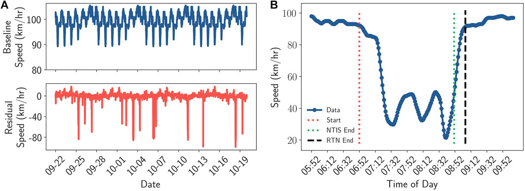
FIGURE 2. The baseline for a single link and an example incident. The baseline captures clear seasonality in the data. On a much shorter time-scale, we see a drop in speed in the wake of an NTIS incident flag, and a recovery after a sustained period of low speed. (A): An example weekly baseline, and residuals (data—baseline) for a single link, showing 4 weeks of data. (B) An example comparison between NTIS end times and the Return to Normal (RTN) end time. We are trying to predict the time until we return to normal operating conditions, rather than the time at which the NTIS flag is turned off.

Using this methodology, we process our dataset such that we have a set of records with the start time of each incident and the time at which the link returned to normal. We include a safety margin in this baseline to account for any persistent but minor problems, shifting it down by 8 km/h ($\approx 5$mph). A link is considered to have returned to normal when its speed is above this shifted baseline for at-least three consecutive minutes, acting as a persistence check.

4 Methodology

Our modeling approach compares multiple methodologies to predict incident durations. A concise summary with all models considered and the main points of note about them is available in the Supplementary Material.

4.1 Incident Features

As discussed, there is much work in the literature identifying the most influential features for incidents. However, we are restricted in two ways. The first is that at any time-step of a prediction, we only incorporate features that would be known at that step. The second is that our dataset does not provide as comprehensive an overview of some features that are likely to be highly informative of the duration, for example we do not have in-depth injury reports or arrival time of police forces. The features we do use are separated into time invariant and time varying categories. The time varying features are derived from time-series of speed, flow and travel-time provided at a 1-min resolution, which we take for the link an incident occurs on. We first remove the seasonality from each of these series by determining “typical weeks” just as in the case of the speed baseline, then subtracting this from the time-series to generate a set of residual series. We then hand engineer features that may be of use for some simple dynamic models, computing the gradient of the residuals at some time t using the previous 5-min of data from t, as-well as simply recording the value of the series. These are used as initial features from the time-series as they provide a sensible and intuitive summary of an incident from the sensors, however of-course more complex features might be derived from the series. We consider models that do just this by applying temporal convolutions across the residual series, and compare the modeling results in section 5.

The time invariant features on the other hand are detailed in Table 1, and are a combination of what an operator might know using existing camera and phone coverage of the SRN. For completeness we also detail the time varying features there also.

TABLE 1

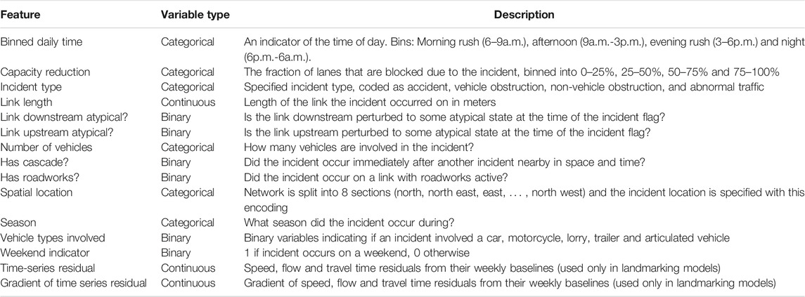
TABLE 1. Overview of the features considered for incident duration modeling. These would be recorded by an NTIS operator when an incident is declared in the system and observed on the network. The time-series features are recorded by inductive loop sensors along the road, and reported each minute. We further consider machine learning models that engineer time-series features automatically.

While not exhaustive, the features in Table 1 offer a combination of contextual information in time, space and specific to the incident. Our choice of bins for time of day reflects typical commuting patterns in the United Kingdom. Some authors use day and night time as separation, as in Zou et al. (2016), where as others account for peak times in their binning Nam and Mannering (2000) and Khattak et al. (1995), as we have. It should also be noted that different incidents may have the same type, for example an accident, but have different severities, and hence different impacts on the traffic flow. We rely on the incident type, number of vehicles involved, types of vehicles involved and the time-series provided by the sensor network to allow the models to have some sense of severity, however one could equally directly provide some measure of severity as an input to the model.

We also recall that here “links” are defined as in the NTIS system, being sections of road that have a constant number of lanes and no slip roads joining or leaving, and hence features based on link measurements are derived directly from the representation of the network used in practical operation. Finally, it was found in Kalair et al. (2021) that a time-scale of 100 min and a length scale of 2 km (upstream of an incident) are sensible criteria for cascading incidents in our dataset. Since we only consider data from one direction of the M25, it is sensible to only consider cascading incidents to occur upstream of original incidents. Strict causality is not determined, however there is implied causality through the assumptions of the model in the cited work. While significant investigation into the exact causality of cascading incidents could be investigated, this is a complex task in its own right and a reasonable but simpler way to incorporate it into our model is to utilize the results found in the existing literature.

4.2 Survival Analysis Methods

We first offer more detail on models in the vein of classic survival analysis that we will consider for our problem. We remind the reader that, following the convention in the survival analysis literature, we use the word “event” to mean the occurrence of the outcome of interest. In our case, this is the end of a traffic incident as determined by the return of the speed to within some threshold difference from the profile value. Survival analysis methods aim to model some property of the duration distribution. Let $f\left(t\right)$ be the probability density function (PDF) of incident durations, and $F\left(t\right)$ be the cumulative distribution function (CDF). A key component in survival analysis is the survival function $S\left(t\right)$, which in our context describes the probability an incident has not ended by time t, where time is measured from the start of the incident. Denoting the event time (the incident end time) by T, we formally write:

$\begin{array}{l}S\left(t\right)=\mathrm{\mathbb{P}}\left(T\ge t\right)\\ =1-F\left(t\right)\\ ={\displaystyle {\int }_t^{\infty }f\left(x\right)dx}\end{array}(1)$

Further, many survival analysis methods are concerned with the hazard function $\lambda \left(t\right)$, describing the instantaneous rate of occurrence of events. One can show that:

$\begin{array}{l}\lambda \left(t\right)=\underset{dt\to 0}{\lim }\left(\frac{\mathrm{\mathbb{P}}\left(t\le T<t+dt|T\ge t\right)}{dt}\right)\\ =\frac{f\left(t\right)}{S\left(t\right)}\end{array}(2)$

In practice, this means that the instantaneous rate of events is equal to the density of events at that time divided by the probability of surviving to that time. A final concept of note is the cumulative hazard function $\Lambda \left(t\right)$, which is the integral of the hazard function between time 0 and t:

$\Lambda \left(t\right)={\displaystyle {\int }_0^t\lambda \left(s\right)ds}(3)$

Using these concepts, the first model we apply is a Cox regression model, reviewed in Kumar and Klefsjö (1994). Suppose some “individual” i (incident in this application) has covariate vector $x_i$. A Cox model specifies the hazard function for individual i as:

${\lambda }_i\left(t|x_i\right)={\lambda }_0\left(t\right)e^{x_i^{\prime }\beta }(4)$

where ${\lambda }_0\left(t\right)$ is some baseline hazard at time t, and $\mathit{\beta }$ is vector of regression coefficients. The baseline hazard describes the hazard function for an individual with covariates all equal to 0, and then it is adjusted for a particular individual with the exponential of the regression term. In this original formulation, the covariate effect is constant in time, but the baseline hazard varies in time. Various methods exist for estimating a baseline hazard function, with more details found in Kleinbaum and Klein (2012). In short, the baseline hazard is assumed to be piecewise constant and determined without any distributional assumptions, allowing the data to construct an approximation. One can determine $\mathit{\beta }$ by optimizing the partial likelihood:

$PL\left(\beta \right)={\displaystyle \prod _{i=1}^N{\left[\frac{e^{{x^{\prime }}_i\beta }}{{\displaystyle {\sum }_{j=1}^N{e}^{{x^{\prime }}_j\beta }{Y}_j\left({\tau }_i\right)}}\right]}^{{\delta }_i}}(5)$

where ${\delta }_i$ is one if the event time is observed and 0 if it is censored and $Y_j\left({\tau }_i\right)$ is one if individual j is still at risk at time ${\tau }_i$. Here ${\tau }_i$ represents the recorded incident duration for incident i. The baseline hazard function can be determined using the Breslow estimator:

${\lambda }_0\left({\tau }_i\right)=\frac{d_i}{{\displaystyle {\sum }_{j\in \mathrm{ℛ}\left({\tau }_i\right)}{e}^{{{\mathit{x}}^{\prime }}_j\mathit{\beta }}}}(6)$

where $\mathrm{ℛ}\left({\tau }_i\right)$ is the set of at-risk individuals at time ${\tau }_i$ and $d_i$ is the number of events that have occurred at the $i-th$ time. We use the implementation of Cox models provided in the R package “survival” Therneau (2015). Ties in event times are handled using the ‘Efron’ method, detailed in Efron (1977), altering the likelihood in Eq. 5.

The next model we apply is an accelerated failure time model (recall AFT from the literature review). Such a model supposes relationships between the survival and hazard functions of the form:

$s_i\left(t\right)=s_0\left(t{e}^{{\mathit{x}}_i\mathit{\beta }}\right),{\lambda }_i\left(t\right)={\lambda }_0\left(t{e}^{{\mathit{x}}_i\mathit{\beta }}\right)e^{{\mathit{x}}_i\mathit{\beta }}(7)$

Here, $s_0\left(t\right)$ and ${\lambda }_0\left(t\right)$ represent assumed baseline survival and hazard forms, and covariates “accelerate” or “decelerate” the survival time of particular individuals. Given an assumed form, for example Weibull, Log-normal or so on with parameters $\mathit{\theta }$, one can then fit this model through maximum likelihood, optimizing:

$L\left(\mathit{\theta }\right)={\displaystyle \prod _{i=1}^N{\left[f\left({\tau }_i\right)\right]}^{{\delta }_i}s{\left({\tau }_i\right)}^{1-{\delta }_i}}(8)$

A common way to interpret the AFT model is as a regression on the log of the durations:

$log\left({\tau }_i\right)={\tau }_0+{\mathit{x}}_i^{\prime }\mathit{\beta }+{\mathit{ϵ}}_i(9)$

where ${\mathit{ϵ}}_i$ is noise, with some assumed form. We implement the models using the R package “flexsurv” detailed in Jackson (2016).

As Cox and AFT models involve, in some way, a linear regression on covariates of interest, they are unable to account for potential non-linear, complex interactions and effects of variables without manual investigation and specification. One way to account for this is to instead use random survival forests (recall RSF from the literature review), which are non-linear models based on an ensemble of individual tree models. The basic idea is as follows. Firstly, one takes a training set and generates B bootstrap samples from it, that is samples with replacement. Each of these samples is used to grow a decision tree, however randomness is introduced in the growing of the tree, by selecting a set of potential split variables at each point in which the tree needs to be split. The optimal split variable from this set is chosen to optimize some survival criterion. One of the most commonly used is the log-rank splitting rule (Ishwaran et al., 2008). The tree is then grown until some criteria is met, either a maximal size or minimum number of cases remaining, and the output at the end of any branch is the cumulative hazard function for all data-points that are placed into that branch when passed through the tree. This process is repeated several times and the collection of trees is referred to as a forest. Each decision tree is a non-linear mapping from input covariates to the output cumulative hazard function, and the collection of many trees acts as an ensemble learner. Ensemble models are known to show promising performance in a range of tasks, and this in addition to the non-linear decision tree models suggests such models may improve upon Cox and AFT models for certain datasets. For our work, we use the R implementation found in Ishwaran and Kogalur (2007).

4.3 Deep Learning Methods

Alternative approaches in survival analysis have focused on applying methods from deep learning to incorporate non-linear covariate effects and behaviors. One of the first such methods was in Faraggi and Simon (1995), where a Cox model was considered, but the term ${{\mathit{x}}_i}^{\prime }\mathit{\beta }$ was replaced with $g\left({\mathit{x}}_i\right)$, which was the output from a neural network given input ${\mathit{x}}_i$. Similarly, Katzman et al. (2018) and Luck et al. (2017) extended the cox model to a neural network setting, however fundamentally such models are still somewhat restrictive in that they assume a form of the hazard function. More recently, Lee et al. (2018) suggested to make far fewer assumptions, and instead train a network to directly model the function $F\left(t|\mathit{x}\right)=1-\mathrm{\mathbb{P}}\left(T>t\right)$, referred to as the failure function. To avoid specifying any particular form of this function, the output space was treated as discrete, defined on times $\left\{t_1,t_2,\dots t_{max}\right\}$. We suppose a single output value in this discrete space at time $t_j$ gives $\mathrm{\mathbb{P}}\left(t_j|{\mathit{x}}_i\right)$ and hence we derive $F\left(t_j|\mathit{x}\right)$ as:

$F\left(t_j|{\mathit{x}}_i\right)={\displaystyle \sum _{t=t_1}^{t_j}\mathrm{\mathbb{P}}\left(t|{\mathit{x}}_i\right)}(10)$

However, we still need to enforce that the output vector actually defines a discrete probability distribution. A natural way to enforce this is apply a softmax function on the output layer, normalizing the sum of the values to one though:

$\sigma {\left(\mathit{z}\right)}_j=\frac{e^{z_j}}{{\displaystyle {\sum }_{k=1}^{t_{max}}{e}^{z_k}}}(11)$

In particular, Lee et al. (2018) considered an application with competing risks, where individuals experienced one of many possible events. Here we consider a simpler case, having only one event (traffic state returning to normal), however the methodology remains consistent in this application. As we are only able to measure if an event has occurred each minute from our sensor data, the discrete nature of the model is not restrictive in our context, yet the non-parametric output is appealing as we have seen in an exploratory analysis (described in the supplementary material) that the data does not appear to be generated from any particular, simple closed form distribution. We adapt our implementation from the implementation found in Lee et al. (2020).

For our implementation, we specify a $t_{max}$ value equal to the longest duration, plus a 20% margin as in the original implementation, and define the output grid at a 1 min resolution. However doing so leads to a very large output space for the model, and could potentially lead to over-fitting. To combat this, we apply dropout after every full connected layer in the network, elastic net regularization on the weights and early stopping based on holdout data. We further consider if a parametric distribution may be sufficiently flexible when attached to a neural network model to perform well in the prediction task. To test this, we build another model as described above, but remove the softmax output layer and replace with with a mixture distribution layer, influenced by Zou et al. (2016). We choose our mixture components to be log-normal, avoiding the other specified distributions for numerical stability. This alters the output size to be $3\times N_m$ where $N_m$ is the number of mixtures, a hyper-parameter to tune.

A final alternative that compromises between the full non-parametric discrete output and the parametric mixture is to allow the output layer of the network to define a set of weights, and construct a probability distribution from these weights using kernel smoothing. Kernel smoothing is a non-parametric technique that aims to construct a distribution by summing a set of kernel functions, evaluated at given data-points. Formally, we can write a kernel smoothed result for some desired point z, with kernel centers $Z_i$ and weights ${\omega }_i$ as:

$\widehat{\nu }\left(z\right)=\frac{1}{h_{bw}}{\displaystyle \sum _{i=1}^N{\omega }_{i}K\left(\frac{z-Z_i}{h_{bw}}\right)}(12)$

Here $h_{bw}$ is the smoothing bandwidth and the kernel $K\left(x\right)$ is often taken to be Gaussian, and the resulting estimate essentially builds a distribution as a weighted smoothed sum over all kernel centers. A point with high weighting will result in a significant amount of mass near this location, and a wide bandwidth will smooth this mass out to the surrounding area. Applying this to our problem, it allows us to avoid treating the output space as discrete, and instead we place a kernel center at each point in the formerly discrete grid, and treat the neural network output (including having a softmax applied) as definitions of the weights ${\omega }_i$. Doing this also enforces some amount of smoothness in the output distribution, determined by the choice of $h_{bw}$. We choose to use a bandwidth of 3 min, which still allows significant freedom to the distribution.

The actual function proposed in Lee et al. (2018) to optimize in order to train the network is a combination of two loss values, the first accounting for the likelihood of the observed data and the second enforcing ordering. The likelihood loss function is given as:

${\mathrm{ℒ}}_1=-{\displaystyle \sum _{i=1}^N\left\{{\delta }_i\text{log}\left[\widehat{f}\left({\tau }_i|{\mathit{x}}_i\right)\right]+\left(1-{\delta }_i\right)\text{log}\left[1-\widehat{F}\left({\tau }_i|{\mathit{x}}_i\right)\right]\right\}}(13)$

where $\widehat{f}$ is the PDF (or PMF in the discrete case) implied by the model output, and $\widehat{F}$ is the CDF or (cumulative mass function in the discrete case) implied by the model output, given a particular input ${\mathit{x}}_i$. This is exactly as in Eq. 8, but taking logs, describing the likelihood of survival data. The second loss function is written:

$\begin{array}{l}{\mathrm{ℒ}}_2={\displaystyle \sum _{i\ne j}1\left({\tau }_i<{\tau }_j\right)\eta \left[\widehat{F}\left({\tau }_i|{\mathit{x}}_i\right),\widehat{F}\left({\tau }_i|{\mathit{x}}_j\right)\right]}\\ \eta \left(x,y\right)=e^{-\frac{x-y}{{\eta }_{\sigma }}}\end{array}(14)$

This loss penalizes the incorrect ordering of pairs in terms of the cumulative probability at their event time. If an incident i ends before j, then we would expect $\widehat{F}\left({\tau }_i|{\mathit{x}}_i\right)$ to be larger than $\widehat{F}\left({\tau }_i|{\mathit{x}}_j\right)$, and if so this pair is considered correctly ordered. Large deviations from correct ordering are penalized by $\eta \left(x,y\right)$. The total loss function is then the sum of ${\mathrm{ℒ}}_1$ and ${\mathrm{ℒ}}_2$. The hyper-parameter grids used for all machine learning models can be found in the supplementary material, and all models are trained using 100 instances of random search.

4.4 Dynamic Methods

To this point, all models discussed in this section have been static, that is an individual has a covariate vector ${\mathit{x}}_{\mathit{i}}$, it is passed through some model, and an estimate of its hazard function, failure function or alternative is attained. However, in-practice our specific application contains a significant amount information that may be useful in determining the duration that is not available at the start of the incident. Such information in the traffic domain is a police report made on the scene, recovery information, and specifically of use to us, the time-series provided by the sensors along the road. A significant incident on a road network could lead to speed drops, flow breakdown and travel time spikes, all of which will be evident when we inspect the time-series as the incident progresses. However, the recovery of the link to normal operating conditions is closely tied to these time-series, firstly through the level of the speed series (as this defines how far from a baseline we are), but one could imagine much richer indicators of traffic state can be mined from them. Recall Figure 2B, we see significant structure in the series, having a linear drop near the start of the incident, an unstable oscillation period at lower speeds, then a recovery to normal conditions. Further examples of these series for incident periods can be found in the supplementary material. A number of methods have been suggested to handle dynamic predictions in a survival analysis setting.

4.4.1 Landmarking

With any dynamic prediction approach, the goal is to provide estimates of a hazard function, survival function or similar at some time t, conditioned on the fact that the individual has survived to time t and any covariates they provide. A simple method to do this is known as “landmarking” and is discussed in Dafni (2011). We note from the outset that landmarking is similar to truncated regression discussed in section 2, however this terminology is consistent with the wider survival analysis literature. To carry out landmarking, one first specifies a set of “landmark times” $\left\{t_{L{M}_1},t_{L{M}_2},\dots ,t_{L{M}_K}\right\}$ at which we want to make dynamic predictions. One then chooses some survival model, for example a Cox model, and the hazard function at landmark time $t_{L{M}_j}$ becomes:

${\lambda }_i\left[t|{\mathit{x}}_i\left(t_{L{M}_j}\right),t_{L{M}_j}\right]={\lambda }_0\left(t|t_{L{M}_j}\right)e^{{\mathit{x}}_i{\left(t_{L{M}_j}\right)}^{\prime }\beta \left(t_{L{M}_j}\right)}(15)$

with $t_{L{M}_j}\le t<t_{L{M}_j}+\text{Δ}t$, for some $\text{Δ}t$ defining how far ahead we are interested in looking. Notice how, compared to Eq. 4, the covariate values ${\mathit{x}}_i$ are replaced with those known at time $t_{L{M}_j}$ and the regression coefficients and baseline hazard can vary based on landmark time. At each landmark time, only incidents that are still ongoing are retained, so the model is therefore conditioned on surviving up to this landmark time. To account for potential time-varying effects and avoid misspecification of the regression parameters, events that occur after $t_{L{M}_j}+\text{Δ}t$ are administratively censored, that is they are marked as censored if they survived past the look-ahead time of interest. Such a model is simple to implement as one can refine the dataset at different times to produce dynamic models. However, as the landmark time grows and less data becomes available, some power may be lost when drawing statistical conclusions. To implement these models, we choose landmark times $t_{LM}$ of $\left\{\mathrm{0,15,30,45,60,120}\right\}$ minutes and horizons $\text{Δ}t$ of $\left\{\mathrm{5,15,30,45,60,120,180,240}\right\}$ minutes and display results throughout section 5. Finally, the landmarking framework can be applied with models other than a Cox model, so we consider both Cox and RSF landmarking models as two candidate dynamic prediction models, with RSF offering a non-linear alternative. The same was done to compare to dynamic models in Lee et al. (2020).

4.4.2 MATCH-Net Based Sliding Window Model

The models considered so far require us to manually engineer features from the time-series variables to incorporate them as covariates. As discussed, we use the level and gradient of the residual series, as these will indicate both how close the link is to reaching standard behavior, and if the situation is getting better or worse. However, gradients computed in short windows can be noisy, yet computed on large windows may lead to significant delay in identifying features. Instead, we would like some automated method that, given a time-series, is able to learning meaningful features from them and incorporate them into predictions. Such a method is proposed in Jarrett et al. (2020), where the authors detail a sliding window model which they name MATCH-Net. We note that the algorithm is designed to make dynamic predictions accounting for missing data, although in our application we do not have missing data so are interested in the dynamic prediction aspect only. In this model, a window of longitudinal measurements is fed through a convolutional neural network (CNN), with the convolutions learning features from the time-series that are then used for prediction of risk in some look-ahead window. The model slides across the data, shifting the window each time, meaning features are updated as time progresses and predictions are also shifted forward. It is upon this we base our sliding window methodology.

Specifically, we take a historical window of length w, and at time t feed the time-series from time $t-w$ to t through a CNN, where the filters in the CNN aim to derive features from the series without any manual specification of what they should be. We then concatenate the features output by the CNN with the time-invariant features, and then pass these through a series of fully connected layers. In Jarrett et al. (2020), the output layer was a discrete space upon which a softmax activation was applied, and we again consider this, a mixture of log-normal distributions and a kernel smoothed output distribution. At each input time, we consider a window ahead of the same length as in the fixed case, and treat w as a hyper-parameter to optimize. Since this model is more complex and has far more parameters than in the former case, we consider the discrete distribution to be piecewise constant for 5 min intervals. As a result, the output space decreases in size by 80% without sacrificing too much freedom. A schematic of the network architecture is given in Figure 3, with the output layer left intentionally vague to be clear that we consider multiple different forms of output.

FIGURE 3

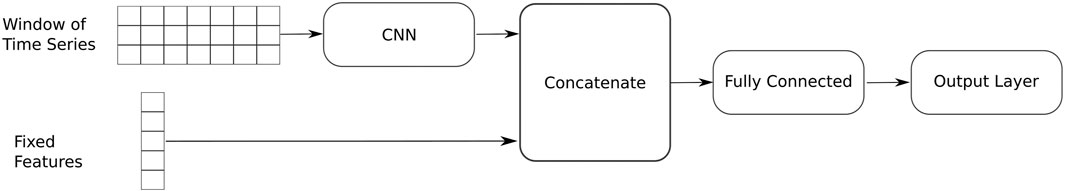
FIGURE 3. Network schematic for sliding window model. We pass filters across the residual time-series to engineer features from each time-series, then concatenate these with the time invariant features to create a feature vector, which is passed through a series of fully connected layers, and some output layer is applied to the result. The example shown is for a single traffic incident being passed through the network. The number of boxes for features is not to scale. The window of time-series represents three variables and a window size of seven in this simple example.

5 Results

A point infrequently discussed in the context of traffic incidents, is that there are multiple criteria that define a “good” hazard model, and multiple ways to measure this in the dynamic setting. We discuss some of these ways in the text below. We note also that elastic net regularization is applied to all deep learning methods, and the optimal Cox and AFT models are selected though inspection of sample-size adjusted Akaike information criterion (AIC) to avoid over-fitting.

5.1 Discriminative Performance—Concordance Index

The concordance index (C-index) has different definitions in the static and dynamic setting. In the static setting, we write it as:

$C=\mathrm{\mathbb{P}}\left[\widehat{F}\left({\tau }_i|{\mathit{x}}_i\right)>\widehat{F}\left({\tau }_i|{\mathit{x}}_j\right)|{\tau }_i<{\tau }_j\right](16)$

Equation 16 is the so called “time dependent” definition used in Lee et al. (2018), accounting for the fact that we care about the entire function $\widehat{F}$ and not a single point value. In the dynamic setting, it is written given prediction time t and evaluation time $\text{Δ}t$ as:

$C\left(t,\text{Δ}t\right)=\mathrm{\mathbb{P}}\left\{\widehat{F}\left[t+\text{Δ}t|{\mathit{x}}_i\left(t\right)\right]>\widehat{F}\left[t+\text{Δ}t|{\mathit{x}}_j\left(t\right)\right]|{\tau }_i<{\tau }_j,{\tau }_i<t+\text{Δ}t\right\}(17)$

The only difference here is now we are specifically computing the C-index at a given prediction time and horizon rather than over the entire dataset, and this is the definition given in Lee et al. (2020). In computing this, we are taking the $\widehat{F}$ values at some time $t+\text{Δ}t$ and compare pairs where an incident i actually ended in the horizon.

As described in Lee et al. (2020), such a measure compares the ordering of pairs. If individual i experienced an event before individual j, then we would expect a good model to correctly assign more chance of an event to individual i than j. A model with perfect C-index, given N traffic incidents, will perfectly predict the order in which the incidents will end. This idea stems from viewing survival analysis as a ranking problem, and since we compare the CDF for two events, we see that it incorporates the entire history from a prediction time up to an evaluation time, not just a single point measurement. A random model will achieve a C-index on average of 0.5, and a perfect model will attain a value of 1.0, so these are reference values to consider when interpreting this measure.

We formally compute Eq. 17 given our dataset by evaluating:

$\begin{array}{l}C\left(t,\text{Δ}t\right)\approx \frac{{\displaystyle {\sum }_{i\ne j}{A}_{i,j}}\cdot 1\left\{\widehat{F}\left[t+\text{Δ}t|{\mathit{x}}_i\left(t\right)\right]>\widehat{F}\left[t+\text{Δ}t|{\mathit{x}}_j\left(t\right)\right]\right\}}{{\displaystyle {\sum }_{i\ne j}{A}_{i,j}}}\\ A_{i,j}=1\left({\tau }_i<{\tau }_j,{\tau }_i<t+\text{Δ}t\right)\end{array}(18)$

where we simply evaluate empirically how often the ordering is correct conditioned on the requirements. The same is true for the static case. If two incidents happen to give exactly the same CDF values when evaluating, we take the convention of adding 0.5 to the total rather than 0 or 1, following the convention in Harrell et al. (1996).

5.2 Calibration Performance—Brier Score

The brier score measures how well calibrated a model is, and compares the binary label (1 if an event has happened at some time, 0 otherwise) with the model prediction at that time. Formally, we write:

$BS\left(t,\text{Δ}t\right)=\frac{1}{N}{\displaystyle \sum _{i=1}^N{\left\{1\left({\tau }_i<t+\text{Δ}t\right)-\widehat{F}\left[t+\text{Δ}t|{\mathit{x}}_i\left(t\right)\right]\right\}}^2}(19)$

where we sum over all events still active at time t, and ask did incident i end before $t+\text{Δ}t$. If it did, then we would expect a good model to have a high CDF value at this point, with one being perfect (i.e., predicting the incident would end by $t+\text{Δ}t$ for certain). On the other hand, if the incident did not end before $t+\text{Δ}t$, then we would expect a low CDF value. This definition is that proposed in the supplementary material of Lee et al. (2020). In a sense, this measures the mean square error of a probabilistic forecast of a binary outcome. In terms of reference values, a model that outputs a survivor function value equal to 0.5 at a particular time will have a Brier score of 0.25, so lower values than this are desirable, and a perfect model will achieve a score of 0.

5.3 Point-wise Performance—Mean Absolute Percentage Error

While C-index and Brier score are used throughout the survival literature, we also note that mean absolute percentage error (MAPE) is used throughout the traffic literature and has some practical relevance to our application. Since we have no censoring, we know the true duration for each traffic incident. As such, we can evaluate for every data-point, what is the error between a point-prediction, and the true duration. A natural choice for such a point prediction is the median of each models output distribution, Yuan et al. (2008), Qi and Teng (2008), Li et al. (2015) as the distribution of traffic incident durations is known to be heavy tailed. We can then ask what is the point-wize error for each model. Note that, C-index and Brier score asked about the accuracy of the output distribution, where as this asks about a single point taken from the distribution. Highways England currently states that NTIS are measured on their prediction of the “likely delay associated with an event.” Specifically, NTIS is scored as follows. One aggregates all incidents that have a predicted return to profile time made at their half way point and lasted over 1 h. The MAPE between these predictions at the half-way point and the true values is computed. The target for NTIS predictions is for this to be below 35%, and it is stated in IBI Group UK (2019) that the current value in practice is 35.49%.

There is of course a problem with this criterion, in that a “perfect” model by this standard would just always predict double the current duration, which would optimize the prediction at the mid-point, but be of no practical use aside from this. Regardless, this rough measure allows us to frame our work in the context of the practical considerations traffic operators are currently working toward.

5.4 Static Prediction Models

We begin by considering how a range of models perform in the static sense. For this, we use only the fixed covariate information available at the start of the incident to fit the models. We apply each of the discussed models, and show results for all metrics in Table 2.

TABLE 2

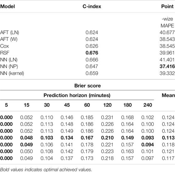
TABLE 2. Performance measures for models in a static setting, where we make only a single prediction per incident using a set of time-invariant covariates. Optimal values are highlighted in bold. AFT (LN)—An accelerated failure time model assuming a log-normal distribution of incident durations. AFT (W)—An accelerated failure time model assuming a Weibull distribution of incident durations. Cox—A linear Cox regression model. RSF—Random survival forest. NN (LN)—A feed-forward neural network model with an output layer that parametrizes a mixture of log-normal distributions. NN (NP)—A feed-forward neural network model with a non-parametric output layer. NN (Kernel)—A feed-forward neural network with a kernel smoothed output.

We see the ordering of incident durations, measured by the C-index, attains values between 0.624 and 0.676. All models are informative, beating the 0.5 reference value, and the biggest gains in C-index are seen when we go from the linear to non-linear modeling frameworks. The RSF achieves the optimal C-index, followed by the neural network with a mixture of log-normals.

In terms of point-wize error, we do not make predictions at the half-way point of incidents, we only make them at the start of an incident in this setting. Doing so and measuring for all incidents longer than 60 min, we see that all models achieve a MAPE between 37 and 41%, with the best model being the non-parametric neural network. No model achieves an MAPE of less than 35%. Finally, the optimal Brier score is always achieved by the RSF method, with the most noticeable differences observed at horizons of 120 and 180 min. There is not much to distinguish many of these models, and ultimately one might suggest that in a static setting, a RSF offers a good compromise between performance measured by C-index, Brier score and MAPE, however if MAPE is the single desired criterion, a non-parametric neural network model would be preferred.

5.5 Dynamic Prediction Models

We now consider the models in a dynamic setting. We consider C-index as defined in Eq. 18, and show results for it at various prediction times and horizons in Table 3. Initially, the RSF achieves optimal C-index across all horizons when predicting at $t=0$. As time of prediction increases, we see a strong favoring of neural network models, specifically the sliding window model with a kernel smoothed output achieves the optimal C-index in most cases. There is a systematic preference for the non-parametric sliding window models compared to others at all prediction horizons when considering prediction times of 30 min or greater. Even at a prediction time of 15 min, the non-parametric sliding window models are preferred when considering 180 and 240 min horizons. As a general summary of Table 3, one should see that out of all 47 prediction time, prediction horizon pairs considered, the optimal model in terms of C-index is the RSF roughly 34% of the time, the sliding window neural network with kernel output 43% of the time, and the sliding window neural network with non-parametric output the remainder of times.

TABLE 3

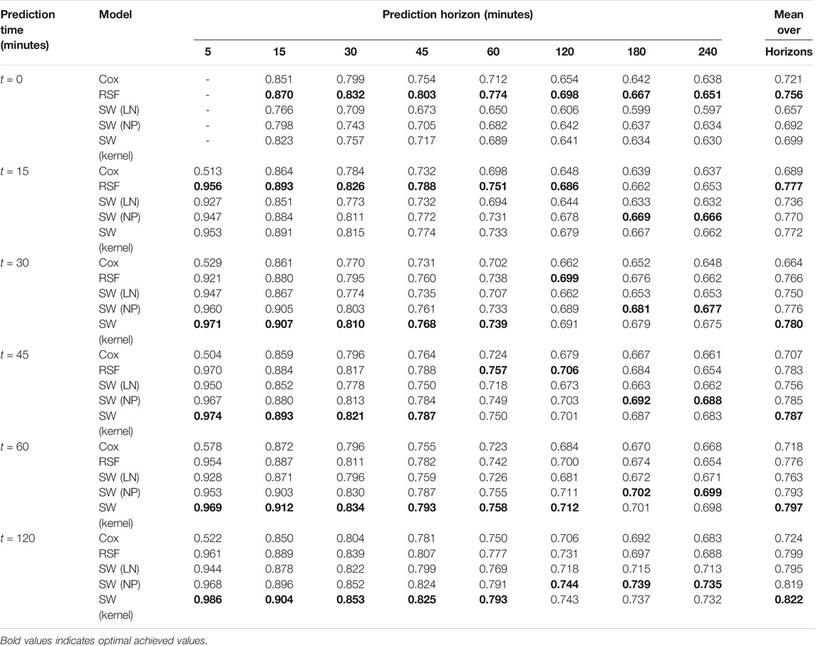
TABLE 3. C-Index values for considered models, across a range of different prediction times (when predications are made) and prediction horizons (at what time after the prediction time they are evaluated). Higher values show a better model. Optimal values for each prediction time—prediction horizon pair are shown in bold. $Cox$—A linear Cox landmarking model. RSF—Random survival forest landmarking model. SW (LN)—Sliding window with log-normal mixture output. SW (NP)—Sliding window with non-parametric output. SW (Kernel)—Sliding window with kernel smoothed output.

Averaged over all horizons, we see that one would prefer the RSF model when initially making predictions, but all prediction times after 15 min favor the kernel smoothed output, with the non-parametric neural network often similar in performance. The neural network model parametrizing a mixture of log-normals achieved the highest C-index of the neural network models in the static case, closely following the RSF model, however it never wins in the dynamic case, suggesting that when we provide the time-series features, the RSF makes better use of them initially, and then the other neural network models make better use of them as time-passes. All models achieve C-index values higher than the reference value of 0.5, across all prediction times and horizons showing their predictions remain informative.

One point of note from Table 3 is that the Cox model has quite poor C-index compared to the alternatives considered when predicting at a horizon of 5 min. We believe this is due to the amount of administrative censoring introduced at such a short horizon. If we look to van Houwelingen and Putters (2012), an assumption of the Cox landmarking model is that there is not too much censoring at the horizon time. For a very short horizon of 5 min, almost all incidents last longer than this, and hence, when we are applying our administrative censoring, this assumption becomes invalid, and we suspect this is why the Cox model has poor results at this horizon.

We further show the Brier scores for each model in Table 4. Again, we observe that initially, the random survival forest achieves optimal scores across all horizons, however as time of prediction increases we gradually see the sliding window neural network with kernel smoothed output start to achieve better Brier scores for short prediction horizons. This is again systematic, and we see for a prediction time of 120 min that the optimal model is the sliding window neural network with kernel smoothed output at horizons up to and including 45 min, but for a prediction time of 45 min it is only optimal for horizons up to and including 15 min. One could postulate that initially, time-series provide less useful information than the fixed features, that is at the very start of an incident, we see only the state of the link before the incident, which might have been reasonably seasonal. However, as time progresses, we will attain more informative features specific to single incidents, and in this case the fact the sliding window method engineers its own features, rather than our noisy gradient and level values we manually input to the RSF model, may prove more useful. Despite this, if a duration is very long, say 4 h, and make a prediction 60 min into it, how much do we truly expect to gain from inspecting the time-series so far? It may be that there is just simply no sign of recovery and all we can really conclude is that speed has been slow for a long time, and shows no other clear features.

TABLE 4

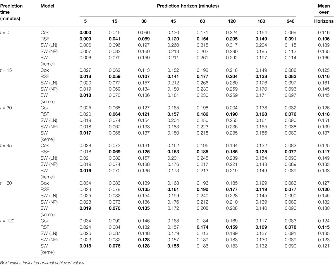
TABLE 4. Brier scores for considered models, across a range of different prediction times (when predications are made) and prediction horizons (at what time after the prediction time they are evaluated). Lower values indicate a better model. Optimal values for each prediction time - prediction horizon pair are shown in bold. All keys are as defined in Table 3.

Another point of note when considering Brier score is that RSF appeared to perform well compared to a non-parametric neural network model in other works. If we look to the supplementary material of Lee et al. (2020), we see that a neural network with a non-parametric output did not consistently improve upon the Brier score achieved by a RSF model (see table VI in the supplementary material of the cited reference). It is unclear therefore if there is some fundamental reason for this in the modeling framework, as two entirely different datasets and applications appear to have observed the same behavior. Despite this, all models achieve Brier scores below the reference value of 0.25.

Finally, we show the error in a point prediction made at various times throughout incidents in Table 5. For reference we also include the value achieved by the fixed model to get an idea of what we are gaining from making dynamic predictions. From Table 5, we see that when making a prediction after 30% of the duration of an incident has passed, we can expect between 30 and 33% MAPE in that prediction. This is around an 5–10% improvement from the prediction made from the corresponding static models at the start of the incident. If we predict half way through an incident, we see that the neural network models all now achieve quite a significantly better MAPE value than the landmarking models, with an optimal MAPE of 21.6% achieved by the mixture of log-normals model, followed by 22% for the non-parametric model. The discrepancy between the sliding window and landmarking models grows as we make predictions later and later, with the sliding window models achieving an MAPE of between 16.5 and 17.3% compared to a value of 26.5% for the optimal landmarking model (RSF). Additionally, the prediction error shows very little improvement moving beyond the 50th percentiles of an incidents duration for the RSF model, and actually increases for the Cox model, suggesting that they are not sufficiently capturing signs in the time-series that indicate the end is near. A key point of practical interest is that with the dynamic models, we do indeed achieve a MAPE value below 35% as desired by Highways England. Of-course, we would need to attain data for all incidents across the United Kingdom to truly ensure that we are able to maintain this on a wider scale, but as far as we are able to measure we achieve what would be considered industrially satisfactory error rates with the dynamic models.

TABLE 5

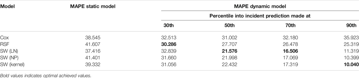
TABLE 5. MAPE at various points for incidents, all of which are at-least 60 min long. The optimal model for each prediction point is shown in bold. The point prediction is generated as the median of the output distribution from each model. All keys are as defined in Table 3.

While the landmarking models appear to plateau in point-wize performance here, we note that it is partly due to plateauing or noisy error they appear to exhibit when making predictions at large landmarking times when only very few incidents remain active. We visualize the error per minute into incidents in the supplementary material, which shows this. The plots within the supplementary material are more akin to something one can find in other dynamic works, for example Figure 2 in Li et al. (2015).

5.6 Do Temporal Convolutions Improve Predictions?

As we have applied methods from Jarrett et al. (2020) to formulate a sliding window model, we have naturally included temporal convolutions to generate information from the time-series. However, a valid question one could ask is are these required in our application, or do the simple levels and gradients retain enough information to make informative predictions? We test this by implementing a model without the CNN structure and instead feeding an input vector consisting of the time-invariant features and the level and gradients computed as in the landmarking case to a feed forward network. Doing so results in a model that achieves a worse Brier score and C-index across all prediction time, horizon pairs and a worse error at the half way point. Exact results are given in the supplementary material.

6 Feature Importance and Model Interpretability

Variable importance is a topic often addressed in the literature, and we offer some discussion of it here for both the RSF model and the non-parametric neural network model, chosen for simplicity compared to the kernel model.

6.1 Random Survival Forest Variable Importance

As RSF are adaptations of random forest methods, standard variable importance metrics are well explored and readily implemented. Recall that trees are trained based on a bootstrap sampled dataset, meaning a set of observations remains for each tree that are “out of bag” which will be used for measuring variable importance. Given a trained forest and some variable of interest x, we drop the out of bag data for each tree down the tree and whenever a split on x is encountered, we assign a daughter node at random instead of evaluating based on the value of x. We then compute the estimates from the model doing this, and the variable importance for x is the prediction error for the original ensemble subtracted from the prediction error for the new ensemble ignoring the x value. A large variable importance suggests that a variable is highly useful in accurately predicting the output. We compute the importance for all features, then scale the importance values by diving by the largest. This yields variable importance on a scale from 0 to 1 and we plot particularly important variables in Figure 4.

FIGURE 4

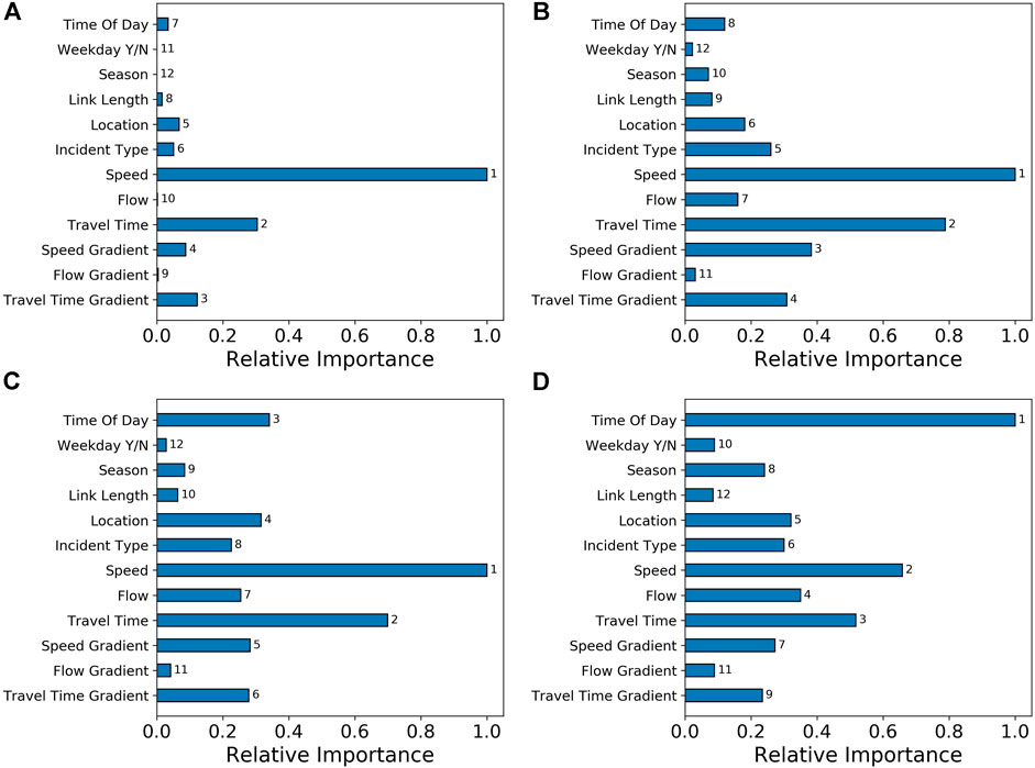
FIGURE 4. Variable importance, as measured for the random survival forest model, for a subset of the important variables. Each plot is a different prediction horizon h, all shown are at a prediction time of $t=30$. The importance at each prediction horizon has been normalized such that the largest importance at any time is 1, and all others are relative to this. The rank of each variable at a given time is written beside each bar. Due to the scaling, one should focus on the ranking and relative difference between bars in each plot. (A): $h=5$. (B): $h=30$. (C): $h=60$. (D): $h=180$.

From Figure 4, we see that the speed value is the most important variable for horizons of 5, 30 and 60 min. At 180 min, the most important variable becomes the time of day. This makes intuitive sense, as we expect the time-varying features to provide more useful information about the immediate future rather than times far into the future. Similar reasoning applies to the importance of travel time and flow. It is interesting to note that flow is often less important than other, time-invariant features, across all horizons. The gradients are always less important than the residual values themselves, which may be a consequence of noise when estimating them, or the fact that the we can see short term rises and falls in the traffic variables that do not indicate the incident is actually near ending, but rather traffic state is just unstable as in Figure 4. The location of an incident is always somewhat important, ranking between sixth and fourth across all horizons. This suggests clear heterogeneity in durations by location. Note that with a location and length, a model should be able to identify single links in the network, so predictions can be specific to these if it improves performance. However, the importance of length decays over horizons, and is always less than the location itself, so the coarse segmentation we have introduced for location seems more important than the specific link an incident occurs on. We see that the season becomes increasingly important as horizon increases. The type of incident varies between the sixth, fifth, eighth and sixth most important variable going from horizons of 5, 30, 60, and 180 min respectively.

6.2 Neural Network Variable Importance

Unlike the Random Forest algorithm, most prediction algorithms do not have a built-in notion of feature importance. This includes the neural network version of the MATCH-NET model developed in Section 4.4.2. Improving the interpretability of neural networks and other general prediction models is a very active topic of current research. See for example Ribeiro et al. (2016) and Shrikumar et al. (2017). We shall use an approach to model interpretation based on a concept called Shapley values borrowed from game theory. For an accessible introduction to these ideas, see Molnar (2019). Shapley values are the fair way to divide a pay-off between coalition members in a cooperative game in which players must decide when to join a coalition in a situation where the payoff depends on the composition of the coalition, Shapley (1953). More recently, Lundberg and Lee (2017) drew an analogy between the contribution of individual players to the pay-off received in a coalition game and the contribution of individual input features to the output of a machine learning model in a prediction task. In this analogy, a single model prediction for a given instance of the feature values is the “game”, each feature value is a “player” and the difference between the prediction for the instance and the average prediction for the entire data set is the “payout”. Shapley values tell us how to fairly distribute the difference between the prediction for this particular instance and the average prediction (the “payout”) among the features, thereby providing an interpretation of the contribution of each feature to the prediction. The sense in which attribution of contributions is fair is based on four properties, efficiency, symmetry, dummy and additivity (see Molnar (2019) for details). Together, these properties provide a reasonable concept of a fair attribution procedure. It can be shown that Shapley values are the only attribution procedure that satisfy all four. From the machine learning perspective, Shapley values are an attractive approach to model interpretability, since it is based on firm theoretical foundations. Furthermore, it was shown by Lundberg and Lee (2017) that many existing model interpretability methods could be understood in terms of Shapley values.

We now provide an outline of how Shapley values are defined and computed. For full details, the interested reader is referred to Molnar (2019) and the references therein. Suppose a model, f, takes, M input features $\left\{x_1,x_2\dots x_M\right\}$. The average prediction of the model is

${\varphi }_0={\displaystyle \int f\left(x_1,x_2,\dots x_M\right)d{\mathrm{\mathbb{P}}}_{x_1,x_2,\dots x_M}}(20)$

where ${\mathrm{\mathbb{P}}}_{x_1,x_2,\dots x_M}$ represents the joint distribution of the feature values in the data. A coalition is a subset of feature values, $\mathcal{S}\subseteq \mathrm{ℳ}$. We denote the size of the coalition by S. The pay-off of a coalition, $\mathcal{S}$, which we shall denote by $V\left(\mathcal{S}\right)$, is the difference between the average prediction, ${\varphi }_0$, and the prediction obtained for the features contained in $\mathcal{S}$ averaged with respect to the features not contained in $\mathcal{S}$:

$V\left(\mathcal{S}\right)={\displaystyle \int f\left(x_1,x_2,\dots x_M\right)d{\mathrm{\mathbb{P}}}_{x\notin \mathcal{S}}-{\varphi }_0}(21)$

The value of adding a new feature, $x_i$, to the coalition $\mathcal{S}$, can now be quantified by calculating $V\left(\mathcal{S}\cup \left\{x_i\right\}\right)-V\left(\mathcal{S}\right)$, the difference in payoffs for coalitions with and without feature $x_i$. The Shapley value for feature $x_i$ is then the weighted sum of this difference over all possible such coalitions:

${\varphi }_i={\displaystyle \sum _{S\subseteq \mathrm{ℳ\setminus }\left\{x_i\right\}}\frac{\left|S\right|!\left(\left|M\right|-\left|S\right|-1\right)!}{\left|M\right|!}\left[V\left(\mathcal{S}\cup \left\{x_i\right\}\right)-V\left(\mathcal{S}\right)\right]}(22)$

The weighting factor is non-obvious and is combinatorial in origin: it ensures that the Shapley value is independent of the order in which features are added to coalitions.

From a computational perspective, there are two problems with Eq. 22. The first problem is that we do not know the marginal distributions of the feature values, ${\mathrm{\mathbb{P}}}_{x\notin \mathcal{S}}$, needed to compute the payoff of a coalition in Eq. 21. The second problem is that the number of terms in the sum on the right-hand side of Eq. 22 grows exponentially with the number of features so direct computation quickly becomes infeasible as the number of features grows. The first problem can be addressed using Monte Carlo integration to estimate the integral. To generate Monte Carlo samples, the feature values in $\mathcal{S}$ are first fixed, and then, for each feature not in $\mathcal{S}$, a data instance is selected at random from the data set and the corresponding feature value is copied to the sample. The second problem can be addressed using an importance sampling procedure devised in Lundberg and Lee (2017) which focuses computational resources on those coalitions that contribute most to the sum on the right-hand side of Eq. 22. This procedure is implemented in the SHAP (SHapley Additive exPlanations) package ², The resulting estimates are referred to as SHAP values and more details are available in the supplementary material. The feature importance results in the remainder of this section are obtained using SHAP.

Our model computes values for each output neuron in the network that correspond to particular horizons. Feature importance analysis assesses how these output value depend on input feature values, rather than assessing how some performance metric changes. As a result, we can investigate the effects of different features on different parts of the output distribution for a single input data-point. First, we consider raw feature importance. That is to say we ask whether a variable has a large or small impact on the output of the model at particular horizons. Some results are shown in Figure 5. We see that for very short horizons (5 min) there are a large number of time-series features with high importance.

FIGURE 5

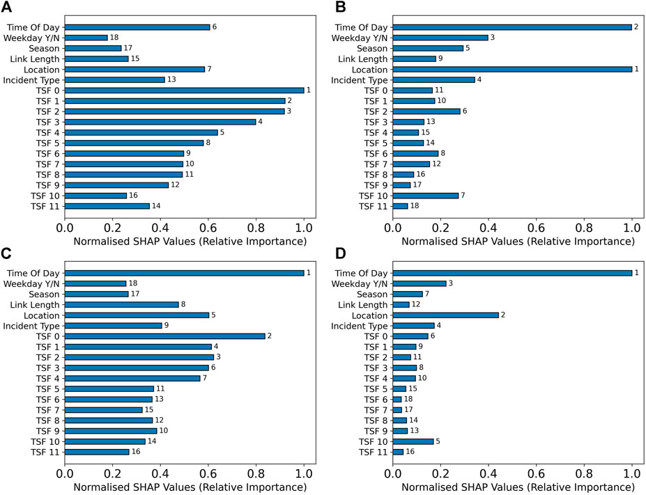
FIGURE 5. Variable importance, as measured for the sliding window neural network model, for a subset of the important variables. Each plot is a different prediction horizon, all shown are at a prediction time of $t=30$. The importance at each prediction time is computed by taking the average of the absolute SHAP values for each feature across all query instances, and then has been normalized such that the largest importance at any horizon is 1, and all others are relative to this. The rank of each variable at a given time is written beside each bar. Due to the scaling, one should focus on the ranking and relative difference between bars in each plot. TSF stands for time-series feature, that have been extracted through passing temporal convolutions across the data. (A): $h=5$. (B): $h=30$. (C): $h=60$. (D): $h=180$.

This makes intuitive sense for the same reasoning as in the RSF case. After the time-series features, we see the time of day, location and incident type are the features with the highest impact. Moving to a horizon of 30 min, we then see the time-series features become less important, and location and time of day dominate the other features. For a 5 min horizon, there were lots of features with quite high importance, showing quite a number influenced the model’s output. In contrast, at a horizon of 30 min we see only these two features with large importance and many others with far less. At a horizon of 60 min, the importance of the time-series features increase again, but the time of day and location remain the two most important of the time-invariant features, ranking first and fifth respectively. One might ask why the time-series features resurge in importance here. This will be explored this further in Figure 6 and the analysis of it. At a long horizon of 180 min, the time of day is by far the most important feature, and the location is second, but is less important relatively than it was at a horizon of 30 min. A natural interpretation of this might be that for long horizons into the future, knowing if an incident will overlap with rush hour or go into lunch time or the night is a good indication of whether we should expect it to last a long time.

FIGURE 6

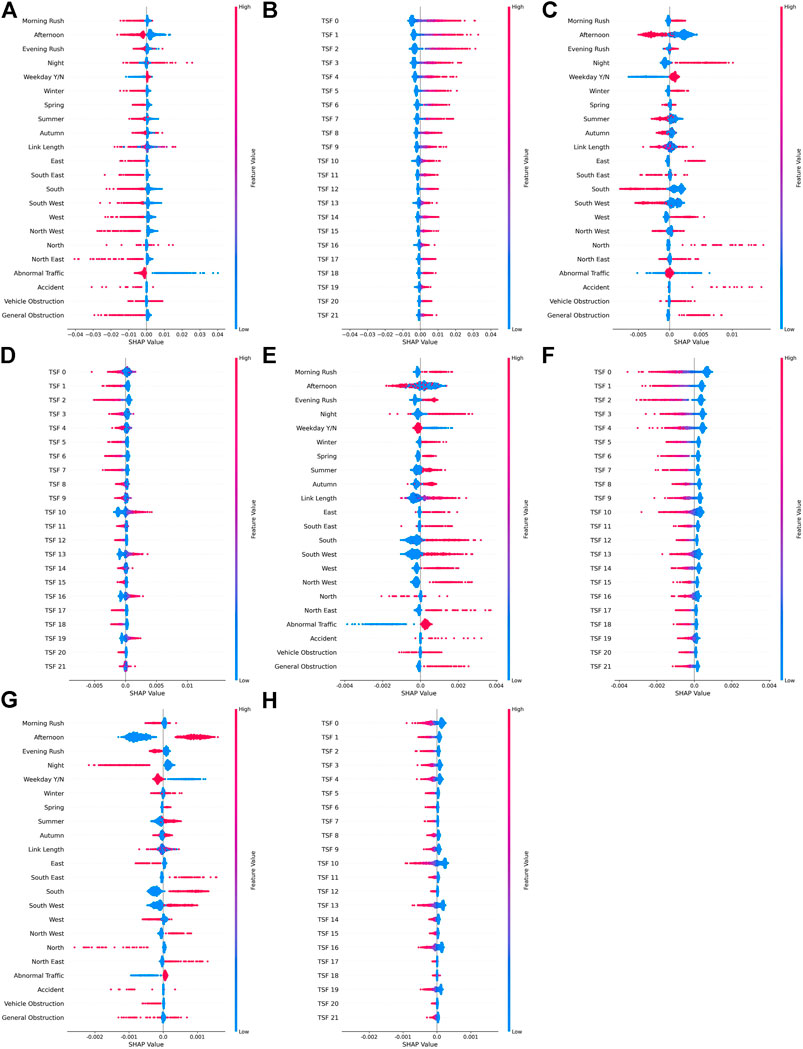
FIGURE 6. SHAP values visualizing how feature values shift the output of the network at particular horizons h. (A): Time-invariant features, $h=5$. (B): Time-varying features, $h=5$. (C): Time-invariant features, $h=30$. (D): Time-varying features, $h=30$. (E): Time-invariant features, $h=60$. (F): Time-varying features, $h=60$. (G): Time-invariant features, $h=180$. (H): Time-varying features, $h=180$.

Having inspected the magnitude of SHAP values, we now look at how different feature values push predicted values up or down. The reader is reminded our model has been trained to predict the probability that an event has ended by a given time horizon. Therefore, “pushing the output up” (a positive SHAP value) corresponds to an increased probability at the given time-horizon. Visualizing this information is quite complex due to the fact that we want to plot the impact of various features, the value they attain, and if this shifted the prediction up or down. One way to do this for SHAP values is using “beeswarm” plots such as those shown in Figure 6. These plots should be interpreted as follows:

• Features of interest are arranged along the y-axis with categorical features like location split into their one-hot encoded states. Each feature has its own beeswarm plot, and within each plot, every data-instance is plotted as a single point.

• The x-axis then displays the corresponding SHAP values which are not normalized as they were in the previous analysis. SHAP values indicate whether a feature shifted the model prediction for that data instance up or down relative to the average prediction.

• The color of a point indicates whether the feature value for that data instance was high (red) or low (blue). For binary features, on is considered high and off is considered low.

• Finally, when many data instances have similar SHAP values, points are expanded outwards on the y-axis. Hence a large vertical strip of points indicates a high density of points at that SHAP value.

The horizon is indicated by h in each sub-caption of Figure 6 and we have split the time invariant features and time series features to aid readability.

There is a large amount of information in Figure 6 and we breakdown the main points here. First consider a horizon of 5 min (Figure 6A,B). There is clear coherence in the features since the colors for any given feature are not randomly distributed. Earlier, we saw time-series features, the time of day and location were influential factors at a 5 min horizon. Considering the time of day in more detail, we see from Figure 6A that when incidents are in the morning rush period (red), the value of the PMF at this time is decreased (negative SHAP value). This indicates that the model predicts it is less likely that incidents at this time of day will end quickly. Moving on to inspect horizons of 30 and 60 min, in Figures 6C,D, we see that that when incidents occur in the morning rush, this increases the output values at these horizons. Finally, more complex behavior is observed at a horizon of 180 min, as incidents occurring in the morning rush sometimes increase, and sometimes decrease the output at this time.

Let us now consider how a location impacts the result. Inspecting the SHAP values for “West”, for example, we see that this feature being “on” (red) decreases the model output at a horizon of 5 min (Figure 6A), increases it at horizons of 30 and 60 min (Figures 6C,E) and then decreases it again at a horizon of 180 min (Figure 6G). Note however that the location feature is categorical and has been one-hot encoded for use with a neural network. As a result, care must be taken in interpreting the impact of the associated SHAP values. The analysis produces a SHAP value for each one-hot encoded value of a categorical feature like location. However, by the nature of one-hot encoding, each data-point has a single location value equal to 1, and the rest equal to 0. So each location feature here will alter the neural network output, but the total impact of a data-point having a particular location will be the sum of the SHAP values for that data-point over all encoded categories. As such, we can better visualize the impact of categorical variables, for example location, by first summing the SHAP values for a data-point for all encoded groups of a particular feature, then visualizing how the overall feature impacted predictions. This is done in Figure 7.

FIGURE 7

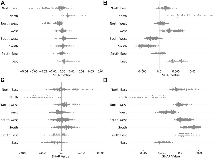
FIGURE 7. SHAP values for the location feature. In each plot, we have summed the SHAP values for each one-hot encoded value, and then only plotted the resulting value in the row corresponding to each data-points true feature value. This shows the overall impact of the location feature, and allows one to view this impact separately for each value it attains. (A): $h=5$. (B): $h=30$. (C): $h=60$. (D): $h=180$.

Note further that the implementation we use when computing these SHAP values accounts for this structure imposed on the inputs. By this, we mean when feature values are copied from background samples in the Monte Carlo sampling, we actually copy groups of features to ensure this structure on the inputs is respected. Considering the location example, this means we do not input data-points to our model that have two locations, and our feature importance respects the practical constraints imposed on the model.

The more intuitive description offered in Figure 7 allows one to see the overall impact of the location variable. Note that the points are no longer colored here as the feature value an incident attains is instead given on the y-axis, with the x-axis visualizing the overall SHAP value for the location variable group. An example interpretation one could read from Figure 7 is: for data-points where the spatial location was east, the overall impact of having this location on the model output was an increase in the output at horizons of 5 and 30 min, and a decrease at 60 and 180 min. From this more refined view, we can see that incidents in the north east are quite varied, as their SHAP values sometimes shift up and sometimes shift down for all horizons. Incidents in the north typically have the output increased at horizons of 5 and 30 min (Figures 7A,B) and then decreased at horizons of 60 and 180 min (Figures 7C,D). This suggests that, for example, the model has learnt incidents in the north are of shorter duration than incidents in the south, however this can then be adjusted further by other observed features. Locations can be compared in this way for all possible pairs.

A further question of interpretability relates to the features engineered from the time-series: what effect do these have on the model? We previously saw that they were highly important at 5 and 60 min horizons, but we can now use Figure 6 to consider what impact they are having. If we start with a horizon of 5 min, we see from Figure 6B that when the time-series features attain a high value, the model output at this horizon is increased. We do not have an interpretable explanation of these features, but we see that they can provide quite significant shifts up in the output if their values are high. Moving to a horizon of 30 min, we see from Figure 6D that the series features become less coherent. Some features attain a high value and shift the output up, others down, and the overall impact is small for many features compared to the impact of the fixed features. This does indicate that the features learnt from the series are distinct in some sense, providing different impacts on the model output. At a horizon of 60 min, we see from Figure 6F that the features attaining a high value indicates a decrease in the model value at this point. From this we can interpret that when high values of features from the are attained, they are making the model put more mass in the immediate future, and less at horizons of 60 min or longer. This is perhaps an intuitive result, that the time-series are providing information that can significantly increase the model output at short term horizons, and attaining these same values shifts down the predictions at long horizons.

Of course, the sheer amount of data available here is somewhat overwhelming, however using SHAP values one can gain a significant understanding of why the machine learning model is outputting particular values. We further show plots for the overall impact of categorical features in the supplementary material, for interested readers, omitted for brevity here. However, care must always be taken in ensuring that feature importance and causality are not assumed, rather we are able to question why the model gives a set of outputs for a particular set of inputs.

7 Conclusion

In this work, we have addressed a number of issues raised in the literature regarding traffic incident duration prediction. Firstly, we considered a method to determine incident duration as not only when an operator declared it cleared, but also when the traffic stated had returned to some typical behavior. This ensured that our predictions reflected when commuters could expect normal traffic conditions to resume if an incident had a significant impact even after it was cleared. Secondly, we considered a range of models, some based on classic survival analysis and others based on machine learning and assessed how they performed on our dataset in both a static and dynamic setting. In-particular, we took inspiration from work in the domain of healthcare and applied emerging methods used there to problems in traffic incident analysis. We saw that in a static setting, there was little to choose between the models but generally either a neural network or random survival forest method would be preferred to the others considered. We moved into the dynamic setting by utilizing landmarking and sliding window neural networks that applied temporal convolutions to the time-series, both of which were inspired by success in healthcare applications. We saw non-parametric methods that made no distributional assumptions were preferred to methods that parametrized mixture distributions, and saw some benefit in applying kernel smoothing to enforce some minimal structure on a non-parametric output. Utilizing models with non-parametric distributional forms was influenced by the increasingly complex distributions being considered for this problem in the traffic literature, and showed significant promise in our results.

We assessed how each model performed using three different scoring criteria and in the dynamic sense, we saw clear structure in the results, with the kernel smoothed neural network model achieving an optimal C-index, Brier score depending on prediction time and horizon as to which model was preferred between a random survival forest and kernel smoothed neural network, and finally saw the neural network models showed much better performance in terms of point-wize error than the comparison models. We saw that all score criteria were improved by engineering features from windows of sensor data through temporal convolutions, compared to feeding in local levels and gradients, suggesting future work should continue to explore methods of deriving features from sensor data rather than inputting raw values.

After, we considered variable importance for our model in the dynamic sense, assessing how the random survival forest and neural network models were influenced by the derived features. While we are aware of variable importance being studied in the traffic literature previously, we are not aware of SHAP values being applied to neural network models for incident duration analysis. Time of day and location were generally important across models, particularly at long horizons, and the time-series features were shown to have significant impact on the neural network output at 5 and 60 min horizons.

Finally, our suggestion to use the output of a neural network to define kernel weights, and from this construct a non-parametric distribution through smoothing was novel in that we are not aware of this being done before to the considered model. It has relevance to other applications, specifically if one requires a continuous distribution to be output, but does not want to make strong parametric assumptions about what form this will take. Further work could be done to consider alternative methods to select a bandwidth when applying this type of model, but the freedom it provides appeared promising on our data. Other avenues for further work include incorporating more features in the dynamic prediction models. In-particular, traffic operators will be able to report when recovery vehicles arrive, police involvement and details from on-site reports. Further, social media and weather data could be collected in real-time. It is likely these will have some predictive power for the duration of an incident, and considering how best to incorporate them is an interesting problem. Finally, from our analysis in section 5 we suspect that if one was able to derive robust, complex features from the time-series and feed them into a random survival forest model, we may see further improvements in the model. One way to do this may be through an auto-encoder framework in which we pre-train a model to determine hidden representations of the series, however it is unclear if these will offer the same predictive power as we have observed from the time-series here.

Finally, we have focused on incident duration modeling on the SRN, a significant component of the United Kingdom transportation infrastructure. One could also ask how to apply our methods onto a broader range of roads, for example those in urban areas. Doing so would likely require alternative data-sources to be processed and collected, as extensive loop sensor coverage may not be available in these domains. One promising candidate is to determine measures of speed, flow and travel time based on tracked vehicles and GPS data, however investigating what penetration rates would still yield informative features during incident times is a further question to investigate. If one were to obtain such data however, our methods could be applied to a wider range of locations. Further, more diverse data may be appealing to incorporate in both the highway and urban domains, for example analysis of video feeds and social media data to gain further insight into incident behavior.

Data Availability Statement

Publicly available datasets were analyzed in this study. This data can be found here: http://www.trafficengland.com/services-info.

Author Contributions

KK and CC contributed to conception and design of the study. KK implemented the models, data-processing and performed the analysis. Both authors contributed to manuscript writing, editing and approved the submitted version.

Funding

This work was supported by the EPSRC (Grant Number EP/L015374/1).

Conflict of Interest

The authors declare that the research was conducted in the absence of any commercial or financial relationships that could be construed as a potential conflict of interest.

Acknowledgments

We thank Steve Hilditch, Thales United Kingdom for sharing expertize on NTIS and United Kingdom transportation systems.

Supplementary Material

The Supplementary Material for this article can be found online at: https://www.frontiersin.org/articles/10.3389/ffutr.2021.669015/full#supplementary-material

Footnotes

¹Technical details of the NTIS data feeds are available at http://www.trafficengland.com/services-info

²Implementation and examples given in https://github.com/slundberg/shap

References

Al Kaabi, A., Dissanayake, D., and Bird, R. (2012). Response Time of Highway Traffic Accidents in Abu Dhabi. Transportation Res. Rec. 2278, 95–103. doi:10.3141/2278-11

CrossRef Full Text | Google Scholar

Chung, Y.-S., Chiou, Y.-C., and Lin, C.-H. (2015). Simultaneous Equation Modeling of Freeway Accident Duration and Lanes Blocked. Analytic Methods Accid. Res. 7, 16–28. doi:10.1016/j.amar.2015.04.003

CrossRef Full Text | Google Scholar

Chung, Y., Walubita, L. F., and Choi, K. (2010). Modeling Accident Duration and its Mitigation Strategies on South Korean Freeway Systems. Transportation Res. Rec. 2178, 49–57. doi:10.3141/2178-06

CrossRef Full Text | Google Scholar

Chung, Y., and Yoon, B.-J. (2012). Analytical Method to Estimate Accident Duration Using Archived Speed Profile and its Statistical Analysis. KSCE J. Civ Eng. 16, 1064–1070. doi:10.1007/s12205-012-1632-3

CrossRef Full Text | Google Scholar

Cleveland, R. B., Cleveland, W. S., and Terpenning, I. (1990). STL: A Seasonal-Trend Decomposition Procedure Based on Loess. J. Official Stat. 6, 3–73.

Google Scholar

Cox, D. R. (1972). Regression Models and Life-Tables. J. R. Stat. Soc. Ser. B (Methodological). 34, 187–202. doi:10.1111/j.2517-6161.1972.tb00899.x

CrossRef Full Text | Google Scholar

Dafni, U. (2011). Landmark Analysis at the 25-year Landmark point. Circ. Cardiovasc. Qual. Outcomes. 4, 363–371. doi:10.1161/circoutcomes.110.957951

PubMed Abstract | CrossRef Full Text | Google Scholar

Ding, C., Ma, X., Wang, Y., and Wang, Y. (2015). Exploring the Influential Factors in Incident Clearance Time: Disentangling Causation from Self-Selection Bias. Accid. Anal. Prev. 85, 58–65. doi:10.1016/j.aap.2015.08.024

PubMed Abstract | CrossRef Full Text | Google Scholar

Efron, B. (1977). The Efficiency of Cox's Likelihood Function for Censored Data. J. Am. Stat. Assoc. 72, 557–565. doi:10.1080/01621459.1977.10480613

CrossRef Full Text | Google Scholar

Highways England. (2017). Strategic Road Network Initial Report. Tech. Rep.

Google Scholar

Faraggi, D., and Simon, R. (1995). A Neural Network Model for Survival Data. Statist. Med. 14, 73–82. doi:10.1002/sim.4780140108

CrossRef Full Text | Google Scholar

Garib, A., Radwan, A. E., and Al-Deek, H. (1997). Estimating Magnitude and Duration of Incident Delays. J. Transp. Eng. 123, 459–466. doi:10.1061/(asce)0733-947x(1997)123:6(459)

CrossRef Full Text | Google Scholar

Ghosh, B., Asif, M. T., Dauwels, J., Fastenrath, U., and Guo, H. (2019). Dynamic Prediction of the Incident Duration Using Adaptive Feature Set. IEEE Trans. Intell. Transport. Syst. 20, 4019–4031. doi:10.1109/tits.2018.2878637

CrossRef Full Text | Google Scholar

Ghosh, I., Savolainen, P. T., and Gates, T. J. (2014). Examination of Factors Affecting Freeway Incident Clearance Times: a Comparison of the generalizedFmodel and Several Alternative Nested Models. J. Adv. Transp. 48, 471–485. doi:10.1002/atr.1189

CrossRef Full Text | Google Scholar

Golob, T. F., Recker, W. W., and Leonard, J. D. (1987). An Analysis of the Severity and Incident Duration of Truck-Involved Freeway Accidents. Accid. Anal. Prev. 19, 375–395. doi:10.1016/0001-4575(87)90023-6

PubMed Abstract | CrossRef Full Text | Google Scholar

Harrell, F. E., Lee, K. L., and Mark, D. B. (1996). Multivariable Prognostic Models: Issues in Developing Models, Evaluating Assumptions and Adequacy, and Measuring and Reducing Errors. Statist. Med. 15, 361–387. doi:10.1002/(sici)1097-0258(19960229)15:4<361::aid-sim168>3.0.co;2-4

CrossRef Full Text | Google Scholar

IBI Group UK (2019). Highways England’s Provision of Information to Road Users. Tech. Rep. Office of Rail and Road and Highways England.

Ishwaran, H., Kogalur, U. B., Blackstone, E. H., and Lauer, M. S. (2008). Random Survival Forests. Ann. Appl. Stat. 2, 841–860. doi:10.1214/08-aoas169

CrossRef Full Text | Google Scholar

Ishwaran, H., and Kogalur, U. B. (2007). Random Survival Forests for R. R. News 7, 25–31.

Google Scholar

Jackson, C. (2016). Flexsurv: A Platform for Parametric Survival Modeling in R. J. Stat. Softw. 70, 1–33. doi:10.18637/jss.v070.i08

PubMed Abstract | CrossRef Full Text | Google Scholar

Jarrett, D., Yoon, J., and van der Schaar, M. (2020). Dynamic Prediction in Clinical Survival Analysis Using Temporal Convolutional Networks. IEEE J. Biomed. Health Inform. 24, 424–436. doi:10.1109/jbhi.2019.2929264

PubMed Abstract | CrossRef Full Text | Google Scholar

Junhua, W., Haozhe, C., and Shi, Q. (2013). Estimating Freeway Incident Duration Using Accelerated Failure Time Modeling. Saf. Sci. 54, 43–50. doi:10.1016/j.ssci.2012.11.009

CrossRef Full Text | Google Scholar

Kalair, K., Connaughton, C., and Alaimo Di Loro, P. (2021). A Non‐parametric Hawkes Process Model of Primary and Secondary Accidents on a UK Smart Motorway. J. R. Stat. Soc. Ser. C. 70, 80–97. doi:10.1111/rssc.12450

CrossRef Full Text | Google Scholar

[Dataset] Kalair, K., and Connaughton, C. (2020). Anomaly Detection and Classification in Traffic Flow Data from Fluctuations in the Flow-Density Relationship. Transportation Res. C: Emerging Tech. 127, 103178. doi:10.1016/j.trc.2021.103178

CrossRef Full Text | Google Scholar

Katzman, J. L., Shaham, U., Cloninger, A., Bates, J., Jiang, T., and Kluger, Y. (2018). Deepsurv: Personalized Treatment Recommender System Using a Cox Proportional Hazards Deep Neural Network. BMC Med. Res. Methodol. 18, 24. doi:10.1186/s12874-018-0482-1

PubMed Abstract | CrossRef Full Text | Google Scholar

Khattak, A. J., Liu, J., Wali, B., Li, X., and Ng, M. (2016). Modeling Traffic Incident Duration Using Quantile Regression. Transportation Res. Rec. 2554, 139–148. doi:10.3141/2554-15

CrossRef Full Text | Google Scholar

Khattak, A. J., Schofer, J. L., and Wang, M.-H. (1995). A Simple Time Sequential Procedure for Predicting Freeway Incident Duration. V H S J. 2, 113–138. doi:10.1080/10248079508903820

CrossRef Full Text | Google Scholar

Kleinbaum, D. G., and Klein, M. (2012). Survival Analys. Statistics for Biology and Health. 3 edn. New York: Springer-Verlag.

Kumar, D., and Klefsjö, B. (1994). Proportional Hazards Model: a Review. Reliability Eng. Syst. Saf. 44, 177–188. doi:10.1016/0951-8320(94)90010-8

CrossRef Full Text | Google Scholar

[Dataset] Lee, C. (2020). Dynamic-DeepHit. Available at: https://github.com/chl8856/DeepHit.

Lee, C., Yoon, J., and Schaar, M. v. d. (2020). Dynamic-deephit: A Deep Learning Approach for Dynamic Survival Analysis with Competing Risks Based on Longitudinal Data. IEEE Trans. Biomed. Eng. 67, 122–133. doi:10.1109/tbme.2019.2909027

PubMed Abstract | CrossRef Full Text | Google Scholar

Lee, C., Zame, W. R., Yoon, J., and van der Schaar, M. (2018). “Deephit: A Deep Learning Approach to Survival Analysis with Competing Risks,” in AAAI. Association for the Advancement of Artificial Intelligence (Palo Alto, California USA: AAAI Press)), 2314–2321.

Google Scholar

Lee, Y., and Wei, C.-H. (2010). A Computerized Feature Selection Method Using Genetic Algorithms to Forecast Freeway Accident Duration Times. Computer-Aided Civil Infrastructure Eng. 25, 132–148. doi:10.1111/j.1467-8667.2009.00626.x

CrossRef Full Text | Google Scholar

Li, R., and Guo, M. (2014). Competing Risks Analysis on Traffic Accident Duration Time. J. Adv. Transp. 49, 402–415. doi:10.1002/atr.1279

CrossRef Full Text | Google Scholar

Li, R., Pereira, F. C., and Ben-Akiva, M. E. (2015). Competing Risk Mixture Model and Text Analysis for Sequential Incident Duration Prediction. Transportation Res. Part C: Emerging Tech. 54, 74–85. doi:10.1016/j.trc.2015.03.009

CrossRef Full Text | Google Scholar

Li, R., Pereira, F. C., and Ben-Akiva, M. E. (2018). Overview of Traffic Incident Duration Analysis and Prediction. Eur. Transp. Res. Rev. 10, 22. doi:10.1186/s12544-018-0300-1

CrossRef Full Text | Google Scholar

Li, X., Liu, J., Khattak, A., and Nambisan, S. (2020). Sequential Prediction for Large-Scale Traffic Incident Duration: Application and Comparison of Survival Models. Transportation Res. Rec. 2674, 79–93. doi:10.1177/0361198119899041

CrossRef Full Text | Google Scholar

[Dataset] Luck, M., Sylvain, T., Cardinal, H., Lodi, A., and Bengio, Y. (2017). Deep Learning for Patient-specific Kidney Graft Survival Analysis. Arxiv paper, http://arxiv.org/abs/1705.10245

Lundberg, S. M., and Lee, S. (2017). A Unified Approach to Interpreting Model Predictions. Proceedings of the 31st International Conference on Neural Information Processing Systems, Long Beach, CA, United States, (Red Hook, NY, United States: Curran Associates Inc.) 30, 4768–4777. doi:10.5555/3295222.3295230

Google Scholar

Molnar, C. (2019). Interpretable Machine Learning. Available at: https://christophm.github.io/interpretable-ml-book/.

Nam, D., and Mannering, F. (2000). An Exploratory hazard-based Analysis of Highway Incident Duration. Transportation Res. A: Pol. Pract. 34, 85–102. doi:10.1016/s0965-8564(98)00065-2

CrossRef Full Text | Google Scholar

Oralhan, B., and Göktolga, Z. G. (2018). Determination of the Risk Factors that Influence Occurrence Time of Traffic Accidents with Survival Analysis. Iran J. Public Health. 47, 1181–1191.

PubMed Abstract | Google Scholar

Peluffo, N. (2015). Strategic Road Network Statistics. Tech. Rep. United Kingdom Department for Transport.

Qi, Y., and Teng, H. (2008). An Information-Based Time Sequential Approach to Online Incident Duration Prediction. J. Intell. Transportation Syst. 12, 1–12. doi:10.1080/15472450701849626

CrossRef Full Text | Google Scholar

Ribeiro, M. T., Singh, S., and Guestrin, C. (2016). “Why Should I Trust You?”: Explaining the Predictions of Any Classifier,” in Proceedings of the 22nd ACM SIGKDD International Conference on Knowledge Discovery and Data Mining (New York, NY, USA: Association for Computing Machinery), 16, 1135–1144.

Google Scholar

Shapley, L. S. (1953). 17. A Value for N-Person Games. Contrib. Theor. Games. 2, 307–318. doi:10.1515/9781400881970-018

CrossRef Full Text | Google Scholar

Shrikumar, A., Greenside, P., and Kundaje, A. (2017). Learning Important Features through Propagating Activation Differences. Proceedings of the 34th International Conference on Machine Learning, Sydney, NSW, Australia, (JMLR.org) 70, 3145–3153. doi:10.5555/3305890.3306006

Google Scholar

Smith, K. W., and Smith, B. L. (2001). Forecasting the Clearance Time of Freeway Accidents. Tech. Rep.

Google Scholar

Tavassoli Hojati, A., Ferreira, L., Washington, S., Charles, P., and Shobeirinejad, A. (2014). Modelling Total Duration of Traffic Incidents Including Incident Detection and Recovery Time. Accid. Anal. Prev. 71, 296–305. doi:10.1016/j.aap.2014.06.006

PubMed Abstract | CrossRef Full Text | Google Scholar

Therneau, T. M. (2015). A Package for Survival Analysis in S. Version 2.38.

Valenti, G., Lelli, M., and Cucina, D. (2010). A Comparative Study of Models for the Incident Duration Prediction. Eur. Transp. Res. Rev. 2, 103–111. doi:10.1007/s12544-010-0031-4

CrossRef Full Text | Google Scholar

van Houwelingen, H. C., and Putters, H. (2012). Dynamic Prediction in Clinical Survival Analysis. Monographs on Statistics and Applied Probability. 1 edn. Boca Raton, FL: CRC Press, 123.

Wang, W., Chen, H., and Bell, M. C. (2005). Vehicle Breakdown Duration Modelling. J. Transportation Stat. 8, 75–84.

Google Scholar

Wei, C.-H., and Lee, Y. (2005). Applying Data Fusion Techniques to Traveler Information Services in Highway Network. J. East. Asia Soc. Transportation Stud. 6, 2457–2472.

Google Scholar

Wei, C.-H., and Lee, Y. (2007). Sequential Forecast of Incident Duration Using Artificial Neural Network Models. Accid. Anal. Prev. 39, 944–954. doi:10.1016/j.aap.2006.12.017

PubMed Abstract | CrossRef Full Text | Google Scholar

Weng, J., Qiao, W., Qu, X., and Yan, X. (2015). Cluster-based Lognormal Distribution Model for Accident Duration. Transportmetrica A: Transport Sci. 11, 345–363. doi:10.1080/23249935.2014.994687

CrossRef Full Text | Google Scholar

Wu, J., Subramanian, R., Craig, M., Starnes, M., and Longthorne, A. (2013). The Effect of Earlier or Automatic Collision Notification on Traffic Mortality by Survival Analysis. Traffic Inj. Prev. 14, S50–S57. doi:10.1080/15389588.2013.799279

PubMed Abstract | CrossRef Full Text | Google Scholar

Yuan, Y. (2008). Prediction Performance of Survival Models. Ontario, Canada: Ph.D. thesis, Waterloo.

Zeng, D., and Lin, D. Y. (2007). Efficient Estimation for the Accelerated Failure Time Model. J. Am. Stat. Assoc. 102, 1387–1396. doi:10.1198/016214507000001085

CrossRef Full Text | Google Scholar

Zhan, C., Gan, A., and Hadi, M. (2011). Prediction of Lane Clearance Time of Freeway Incidents Using the M5p Tree Algorithm. IEEE Trans. Intell. Transport. Syst. 12, 1549–1557. doi:10.1109/tits.2011.2161634

CrossRef Full Text | Google Scholar

Zhang, H., and Khattak, A. J. (2010). Analysis of Cascading Incident Event Durations on Urban Freeways. Transportation Res. Rec. 2178, 30–39. doi:10.3141/2178-04

CrossRef Full Text | Google Scholar

Zou, Y., Henrickson, K., Lord, D., Wang, Y., and Xu, K. (2016). Application of Finite Mixture Models for Analysing Freeway Incident Clearance Time. Transportmetrica A: Transport Sci. 12, 99–115. doi:10.1080/23249935.2015.1102173

CrossRef Full Text | Google Scholar