Effectiveness of Free Bikes and E-Bikes for Commute Mode Shift: The Case of Google’s Lending Program

1 Introduction

Barriers to bike commuting are well documented. Concern for traffic safety and distance (or travel time) top the list as some of the strongest (Dill, 2009; Heinen et al., 2010; Xing et al., 2010; Fowler et al., 2017). While improving street design for bicycling is badly needed in most United States cities, education, encouragement, and incentive schemes within transportation demand management (TDM) programs can provide synergistic benefits for increasing bicycling by focusing on reducing other barriers (Litman, 2021).

Bike ownership is a prerequisite for bike commuting (except in locations with one-way bike shares) and has been shown to be strongly correlated with bicycling in general (Handy et al., 2010). Other than the cost burden of purchasing a bike, little is known about the motivations for acquiring a bike. In at least one study, evidence suggests that socio-demographics and travel attitudes influence bike ownership, but the direction of causality is not clear (Ramezani et al., 2021). In many studies of bike commuting, bike ownership is assumed to be jointly made with the decision to commute by bike (i.e., if someone decides to bike commute, they will buy a bike to do it). However, this assumption is particularly problematic if barriers to ownership preclude people from considering bike commuting.

Electric assisted bikes (e-bikes) have been shown to strongly increase bicycling and decrease driving, more so than conventional bikes (Fitch, 2019). E-bikes afford greater commute distances because riders can travel at faster speeds with less effort, which is especially true of hill climbing. This travel time reduction can make e-bicycling more competitive with driving in many environments, and for shorter commutes often makes e-bicycling the fastest door-to-door commute mode. E-bike lending has been examined in a variety of contexts, but perhaps the best available evidence comes from studies in Norway. In a series of studies with brief e-bike lending periods, large increases in bicycling and reductions in driving were found (Fyhri and Fearnley, 2015; Fyhri et al., 2016; Fyhri and Beate Sundfør, 2020). In less robust evaluations, several European studies in the grey literature have demonstrated large increases in bicycling and decreases in driving, the latter of which is particularly apparent for commuting purposes (Haubold, 2016; Fitch, 2019). While the evidence is less clear in North America, from the few available studies, consistent with the European experience, e-bike owners replace driving for a large percentage of trips (Lamy, 2001; MacArthur et al., 2018). The potential for e-bicycling to substitute for driving is perhaps greater in North America where driving is a more dominant travel mode. This is especially the case for commuting to work. While e-bikes hold promise for increasing bicycling, conventional bicycles are still the dominant form of bike commuting in the United States. Conventional bicycles have a few important advantages (e.g., less expensive, less prone to theft, less maintenance costs), and for those who seek a commute that also satisfies fitness goals, conventional bicycling does require more energy expenditure [e-bikes still provide important health benefits, see Sundfør and Fyhri (2017)].

While e-bike and bike lending have been a part of some employer-based and university TDM programs in the United States, there have been few evaluations of their results. In one university bike lending program, bicycling to campus rose but had little effect on car use (Armstrong, 2010). A much smaller lending program (30 bikes, 10-week lending period) to three large employment campuses in Portland, Oregon showed substantial increases in bike use (MacArthur and Kobel, 2016). However, that study included mostly existing bike commuters, had no regularly reported trip data (only one mid-program survey), and the sample size for some evaluations were very small (e.g., n = 37 for mid-program bicycling use). The lack of robust bike lending evaluations is likely due to the rarity of the programs in the United States, but also due to the challenges of evaluating real-world TDM programs. Bike and e-bike lending programs are often one facet of a broad suite of programs to encourage reduction in driving or other related TDM goals. For example, evidence suggests that policies that combine education and encouragement interventions with infrastructure investments see synergistic effects (Pucher et al., 2010). Along with encouragement/education campaigns, regular and ongoing monetary incentives are another potential synergistic option. For example, a study of a TDM program to decrease peak car travel to a large college campus showed that monetary incentives can strongly influence travel behavior (Zhu et al., 2015). Not only can incentives be synergistic with mode expansion (e.g., bike lending), but so can disincentives for driving. The high societal cost of providing free parking has been well documented (Shoup, 1997b) and many TDM strategies to reduce single occupancy commuting are thwarted by plentiful parking (Nozick et al., 1998). Until parking costs are borne on commuters, TDM strategies are essentially competing against car commuting subsidies in the form of free parking. Given the rising value of urban land making parking extremely costly, successful parking cash out reforms (Shoup, 1997a) are likely to form a strong synergy with bike lending in getting more people to consider bike commuting. However, evaluations of these potential synergies are needed.

One-way bike shares are another potential strategy to reduce the burdens of owning and operating a bike for commuting. Bike shares operated by or for cities typically have commute users, but corporate bike share (like the one at Google) are not designed for commuting. Instead, they are designed for trips between buildings on the corporate campus or to nearby locations during the workday. So while city-level bike shares could be a good investment to spur bike commuting, corporate bike shares haven’t historically had operational areas that have allowed them to be used as a commute strategy.

In this study we focus on evaluating the effectiveness of a large (possibly the largest) employer sponsored (Google) bike and e-bike lending program in North America. We have two primary research questions: 1) how did the lending program effect bike commuting? And 2) how did the lending program effect single occupancy vehicle (SOV) commuting? We also examined other factors that provide insight into the program effectiveness and discuss the potential for bike lending as a strategy for other large employers to achieve similar goals. To our knowledge this is the first large scale evaluation of a corporate commuter bike lending program in North America, so it is expected to spur more programs and more research on this topic.

2 Materials and Methods

2.1 Case Study: Google Bike Commuter Program (Bike and E-Bike Lending)

Google’s headquarters, where most of its employees commute daily (prior to the COVID-19 pandemic), is in two suburban office parks: one in Mountain View and the other in Sunnyvale, CA, United States. Both office parks were originally designed to prioritize vehicular travel, but Google uses TDM strategies to increase the sustainability of its workforce’s commuting, including its commuter shuttle program (GBus), subsidized public transit passes, free bikes, vanpools and microtransit options, and subsidized carpool rides. Although parking is also free and available on a first come, first serve basis, less than 50% percent of Google employees commute by single occupancy vehicle (SOV), and the bike mode share is roughly 5–6 percent of commutes.¹

As part of their TDM program, Google sought to increase their near-term bike commuting mode share to 10%, with a long-term goal to reach 20%. Following an initial survey of bicycling to campus which indicated bike ownership and worry about maintenance were primary bike commute barriers, Google began a pilot program that loaned high-quality electric-assisted bicycles to use at no cost to interested employees. Included in the offering was free maintenance, helmet, lock, lights, and emergency van pick-up or drop off service. As the pilot program grew in popularity and success, it became a full program that required participating employees to commute by bike for 60% of their commute days and log their commute trips. At the end of the six-month program, participants received a $300 subsidy to purchase a bike (or e-bike) in addition to discounts from participating local bike shops during sales events held on campus and at bike shops directly. Over time, the lending program has grown to include more than 2,600 participants since 2015 (the beginning of our study period) and has included many changes to the program including expanded bike options (non-electric commuter bike) and participation through the end of 2019 [see Fitch et al. (2022) for more program details]. The program continued to evolve throughout the years as program managers received feedback and learned from participants. A six-month lending period was used based on evidence that suggests that many habits take a long time to form (Lally et al., 2010). Some of the selection criteria and rules for the program targeted employees who commonly drove to work, did not have access to a working bicycling, lived within 20 miles from work, had a safe place to lock their bike at home, agreed to program audits and surveys.

2.2 Data

We synthesized anonymized survey and trip data collected as a part of the program operations and compliance and summarized the trip data at the person level in three phases: before program participation (before), during program participation (during), and after program participation (after) (See Table 1). Trip data was collected by Google in one of two ways: 1) self-reported daily commute data (reported every month) through an online form, or 2) use of an integrated smartphone app (Strava). Participants who chose to report trips through Strava had each commute distance measured by the Strava app, otherwise participants’ commute distance was self-reported at the beginning of the program and assumed to be constant through the life of the program unless reported to have changed by the participant. We included all program participants who recorded trip data during the program in this study and retained trip data within 1 year prior to and any time during and after graduation from the program. Trip data was only required for the during phase (while employees were loaned a bike) which is why the unique person-commute days for the before and after phases are much lower (Table 1).

TABLE 1

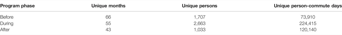
TABLE 1. Sample size by evaluation phase.

To administer the program, Google collected data from participants in two surveys, an application survey (before program enrollment) and an exit survey (after program graduation). Because the program went through many changes from launch in 2015 through the end of this study period (December 2019), the survey data from different date ranges required some synthesis and organization. In total, application survey data was stored in six spreadsheets, and we merged questions with slight changes in wording where possible (see Supplementary Material for details). Most application surveys included key variables in the modeling and analyses. The primary variables in the application data are anonymized person id, application date, primary mode, weekly frequency for each mode, commute distance, and commute time. Nearly all participants reported all these variables in our study sample (82 percent of study participants had some application survey data), but the same is not true of the exit survey. Only 34 percent of study participants completed the exit survey. This is likely because the participant already received their bike subsidy and graduated from the program prior to being recruited to take the exit survey. For this reason, we only use exit survey data for ancillary analyses, not for the primary program evaluation. The exit survey asked many questions about the program and collected comparative commute data, such as primary mode, commute time, and bike frequency before and during the program.

In addition to survey data, data on when participants received a bike and when they graduated from the program was used to help define person-specific study phases (before, during, and after) described below in data cleaning and pre-processing.

2.3 Data Cleaning and Pre-Processing

We cleaned and organized the raw data into person level and trip level data for the primary analyses. We synthesized the raw trip data into commute data by examining trips within normal commute time windows to Google’s two campuses. Because compliance was conducted at the commute level (to and from work) we summarized trips into morning and afternoon commutes by time of day. For our analysis, trips during the mid-day and evening periods were ignored. We explored the differences between morning and afternoon commute mode patterns and found them to be nearly identical (only rarely were participants commuting by different modes within a day). Because of this pattern, we chose to focus on morning commutes only for this evaluation. Within some morning periods, participants traveled by multiple modes (e.g., biked and took GBus to work). We wrote a rule-based algorithm based on timestamps of different modes to determine if people were making multimodal morning commutes and classified them as such. We inferred the use of an integrated app by the number of digits recorded for the trip distance, which likely indicated whether the trip was recorded manually or using an app.

We determined the person-specific program phase (before, during, and after) based on the bike issue and return dates, and graduation² date. Because of missing data for some bike trip logs and graduation, we had four scenarios for determining program endpoints (all participants had bike issue dates that determined program start point): 1) if the participant had a bike return date, those were used, 2) if the participant had a missing return date, but had graduation data, the graduation date was used as the endpoint; 3) if return and graduate date were missing, but the exit survey was available, the eligible subsidy date was used as the endpoint; 4) if none of the above dates were available, the endpoint was assumed to be 6 months (the normal length of the lending period) after they were issued a bike. All participants recorded trips during the program, but only some participants recorded trips before and after the program (Table 1). The reasons for recording trips before and after the program are likely for concurrent TDM programs such as obtaining other commuter benefits,³ but because we do not know the motivation for each person, we did not speculate on other policy variables in our analysis.

Because of the large amount of the data (Table 1) and the focus of our analysis on the general program evaluation, we aggregated daily commute data for modeling. First, we aggregated workdays at the month level (subtracting holidays, out-of-office, and telework) to estimate physical commute days per month per participant. At the month level (e.g., March 2017), some level of seasonality and some level of specific weather events are adjusted for in our analysis (e.g., a historically rainy May 2018). The process of cleaning and synthesizing data is summarized in Figure 1. We also removed trip data that occurred more than 1 year prior to the start of the bike lending period. We did this because in our summary statistics we noticed many participants had biked to work many years before the program, but not within the immediately preceding year. This decision makes our evaluation of behavior change from trip data based on the most recent prior year of travel.

FIGURE 1

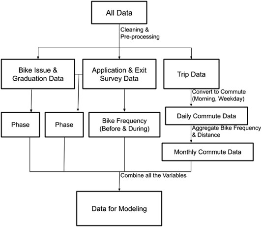
FIGURE 1. Data cleaning and synthesis process.

2.4 Analysis

We found no prior studies that evaluated bike lending within TDM. While some small sample size studies of e-bike interventions had reliable measures of travel and included a control group (Fyhri et al., 2016; Fyhri and Beate Sundfør, 2020), their methods were designed to take advantage of their data and control group [e.g., used one-way between groups analysis of variance (ANOVA)]. In our case, our data has more uncertainty, the study was not designed as an experiment (we treat it as such post-hoc), and our sample size was considerably larger. Because of these differences, we chose to analyze our data using the following methods. We evaluated the program by first reporting bivariate statistics of the outcome variables (bike and SOV commuting rates) with key control (e.g., distance) and program variables (phase). These statistics help indicate the expected program effect and ground the latter multivariable analyses. After the bivariate statistics, we use generalized linear modeling to evaluate the outcomes that considers the complexity of the data as it was generated, the unique variation by each participant, and adjustments to the estimated program effects based on key variables such as bike-type and commute distance. Specifically, we estimate multilevel (by person and by year-month) zero-inflated aggregated binomial regression models. Conceptually the binomial models estimate the likelihood of a participant bike (or SOV) commuting on a given day in each year-month they reported commuting. Because the data has more zero bike (or SOV) days than would be expected from a binomial process, we included a parameter to inflate the zeros to better ensure our model estimates are not upward biased (See Supplementary Material for modeling details). We suspect the added number of zero days is due to people reporting no bike commutes for days in which they never commuted (e.g., non-reported vacation or work-from-home), but the extra zeros could have arisen from other unknown reasons.

Only some participants provided data on SOV commuting as it was not required as a part of the program to report all modes of travel. Therefore, we had less data to model the effect of the program on SOV commuting and SOV commute mile reduction. To ensure we didn’t include people who irregularly reported non-bike trips, we used the following constraints to subset the data: 1) a participant must have at least 8 weeks of commute data that includes all travel modes during the program, and 2) the 8 or more weeks with all commute modes must be 10% or more of a participant’s total reported weeks during the program. These constraints help ensure that we only consider data where SOV commutes are being reported by participants and resulted in a sample size of 893 participants with 99,498 total person-commute days.

2.5 Limitations

The primary limitations for evaluating this program derive from the lack of repeated and objective data on travel before and after the program. This is a problem that plagues many TDM programs because evaluation of program effectiveness is often a lower priority compared to implementation, and because the requirements for conducting high quality evaluations can (and likely do) influence the program and lead to inequities in implementation.

In this study, the before and after trip data are likely biased for several reasons. The before trip data is likely biased to those already bicycling to work (76% of the participants that report before data report at least one bike trip before the program while 78% of participants report never bicycling in the before survey), a sub-sample that is not the primary target for the program. The after-trip data may also be similarly biased (97% of the participants that report after-data report bicycling while only 76% of participants in the exit survey continued to bike). However, the exit survey was completed by so few participants (34%), it makes the survey responses unreliable estimates of the entire program. This is partly because the exit survey was initially only designed for those who did not graduate, but later adopted for all participants. Even though the responses are few, they do allow for trip reporting validation at the person-level. Even trip data during the program has its limitations. Many person-weeks had completely missing data and we were not able to determine if this was because the participant forgot to submit data or didn’t travel to work that week. We ignored these weeks in our analysis which may have led to unknown biases.

We used the before survey data on commute behavior, but that data is likely downward biased from people underreported bicycling behavior prior to the program to get a bike. We assumed that the before trip data was more accurate at the person level (not population) and calculated two versions of the program effects: 1) model predicted differences between phases based on reported trip data, and 2) a comparison of before survey data with model predicted during and after rates from trip data. Each estimate has potential error and bias, and the “true” program effect is likely to be somewhere in-between these estimates. For SOV commutes, we only consider the before survey data with the model predicted during data as the sample size for before and after SOV commute data was very small.

During the bike/e-bike lending program, the commute rewards program was also running, and many people chose to participate in both. We attempted to account for the combined programs versus unique programs, but because it was not feasible to obtain dates for when people were trying to accumulate commute rewards points (we only knew who had ever redeemed a reward during the entire study period), it made differentiating the effects of the lending program and the rewards program impossible. Because the rewards program was available to all participants during this study, we assume that the effects we observe for the lending program are in fact the effects of the combined programs.

Finally, several important person-level variables are absent from this dataset. Most notably, Google does not collect information about socio-demographics, household structure, or any other travel that is not commuting. These and other variables we assume did not bias our effects analysis but since we could not account for them, they are of concern and should be controlled or measured in future evaluations.

2.6 Data Reliability

Most of the data summarized and modeled in this report is self-reported. While a small fraction of participants chose to link a smartphone app to their account to automatically record bike trips, the vast majority manually reported commute diaries monthly. Manual commute diaries are subject to unknown error, and since participants were required to bike 60% of their time to be in program compliance, participants may have over reported their bicycling during the program. However, a comparison between the people who used the smartphone app integration vs. those who manually reported their trips showed very similar results, suggesting the manual reporting bias may be small. Additionally, many participants self-reported bicycling less than was required even knowing the requirement, another indicator of potentially small bias in bike commute data. This may be in part explained by the fact that while participants were expected to commute 60% of the time with their bike, non-compliance was only acted upon when the biking rate dropped below 50%.

We performed one check on the reported bike commute data during the program by comparing it to the self-reported general bike commuting in the exit survey. We found that the exit survey participants reported more bicycling than they did with their trip data during the program (by about 44% on average). However, the sample size was small for the exit survey (since it was voluntary) and so we are less sure this average generalizes to the entire participant population. Because the exit survey suggested the bike commute data during the program was under reported; or perhaps the other way around, the exit survey was overreporting the actual bike commuting, we chose not to make any adjustments to the trip data.

Because of all these reasons, we made no adjustments to the bike commute data for the during and after phases of the program. However, the self-reported bike commute data before the program was subject to different biases. The before bike data may have been improperly deflated by potential participants who may have thought that they wouldn’t receive a bike or e-bike if the TDM managers knew they already bike commuted semi-regularly. In fact, for the small subset of participants who logged commute trips before the program (within 1 year from the start) self-reported much fewer bike commutes in the application. The error is primarily due to the large number of participants reporting never biking to work but who with trip data reported bike trips for other reasons. The reported general bike commuting before the program is downward biased by 19% on average, or the trip data is upward biased by the same amount, or the true bias for each is somewhere in-between.

Finally, we examined the accuracy of self-reported commute distance by comparing with the Strava estimated commute trips for the select participants who used Strava. Figure 2 shows that self-reported commute distance accurately represents mean commutes, but considerable variation in commute distance (perhaps from trip-chaining or detours for exercise) is not accounted for when only reporting “regular commute distance.” Importantly, the self-reported commute distance was done based on driving for most participants, so the comparison between self-report and Strava calculated distances is not entirely apples to apples since bike routes could deviate from car routes substantially.

FIGURE 2

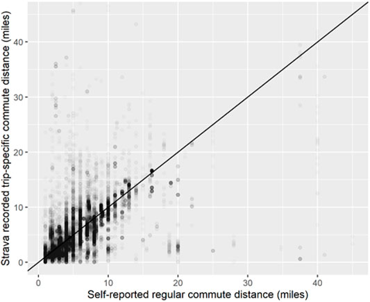
FIGURE 2. Self-reported vs. Strava measured commute distance.

3 Results

3.1 Bike Commute Summaries

Person-averaged weekly morning bike commutes are plotted in Figure 3 for each project phase. The number of participants with data for during-phase commutes was much greater than the other phases due to the commute reporting requirement of the program, hence the smoother histograms in Figure 3. However, even with differences in reporting, the trends in weekly bicycling suggest the program greatly increased bicycling and sustained it after the program. Only the before-phase panel shows many commuters with a zero or near zero weekly bike commute average, and while the during-phase shows the most bike commuting, the after-phase maintains much of the same distribution. The outlying spikes in the histogram during the before and after periods, except for the spike at zero, are from people who reported less than 3 weeks of travel during those periods and are not likely reliable person level means.

FIGURE 3

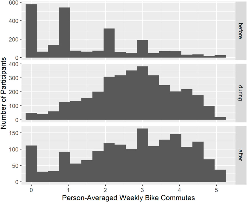
FIGURE 3. Histograms of person-level average weekly morning bike commutes by project phase.

Figure 4 shows the distributions of bike commutes by project phase like Figure 3, but also by self-reported general weekly bike commuting at the time participants signed up for the program (before data from the program application). While Figure 4 suggests the participants who were bicycling 3+ days per week before the program biked the most during the program, the group that never biked before ended up with the largest bicycling increases, biking between 3 and 4 days a week in the during and after phases of the program (just like the 3+ before bike commuters). The last panel of plots in Figure 4 shows the participants who didn’t report their prior bicycling. While they are a substantial fraction of the participants, they biked at slightly less rates on average, like the participants who reported 1–2 days of bicycling before the program. Like in Figure 3, the results in Figure 4 do not account for factors other than the program itself and show similar outlying spikes for people with less than 3 weeks of reported travel in the before and after phase. However, the group means (dashed lines in Figure 4) suggest the greatest program gains are from the participants who never bike commuted prior to the program. Those that already biked 3+ times per week saw very little boost to their bike commuting on average.

FIGURE 4

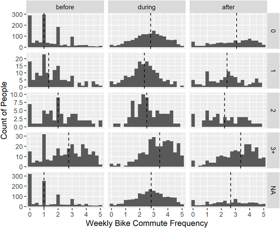
FIGURE 4. Histograms of person-level average weekly morning bike commutes by project phase (row panels) by self-reported bike commute frequency (column panels) before participation. Dashed vertical line is the group mean.

Although the program targeted non-bike commuters, the data in Figures 3, 4 suggest many participants did bike commute prior to the program. The non-zero values in the top left panel of Figure 4 are most surprising since those are people who self-report to never bike commute when filling out the program application. Those non-zero values could have been due to those respondents having bike commuted at a prior time (before application), or they could be people providing false information about their bike commutes to increase their chances of being accepted to the program (see Section 2.6 on data reliability).

Bike commuting by program participants was predominantly done as a direct single mode commute. Less than 10 percent of participants ever made multimodal commutes, and multimodal commutes were a very small share of total recorded commutes (1%). The small share of multimodal commutes was primarily because the program disallowed the e-bikes on GBus and transit because of their weight. Only 18 of the 2,712 participants made 80% or more of their bike commutes as multimodal trips. This is important to consider because even though the behavior is rare, those people who did make multimodal commutes with their conventional bikes, bike commuted more often (see Section 3.2 below).

3.2 Modeling Results

The model results (as logit parameter summaries) are presented in Table 2. The large values for the during and after phases suggest the program substantially increased bicycling to work for program participants. However, because of the potential biases of the data and the complexity of two and three-way interaction effects, we rely on predictive plots for most model inferences. Person-level variation in biking to work is much larger (more than three times) than monthly-level variation (Table 2). We assume monthly level variation is determined largely by weather patterns and seasonal vacationing (Figure 5). Also, person-level variation in average bicycling to work is about the same as the person-level variation in the effect of the program on bicycling to work (Table 2). This suggests that it is not a small subset of highly motivated participants that are making the program successful, but instead the program works for a wide variety of participants. Finally, program participants who didn’t bike much before the program saw much larger effects of the program since the correlations between before- and during-phase as well as the before- and after-phase were strongly negative.

TABLE 2

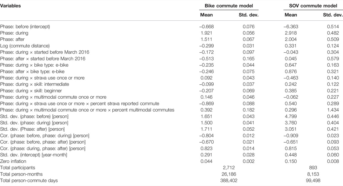
TABLE 2. Zero inflated aggregate binomial bike- and SOV-to-work model summaries.

FIGURE 5

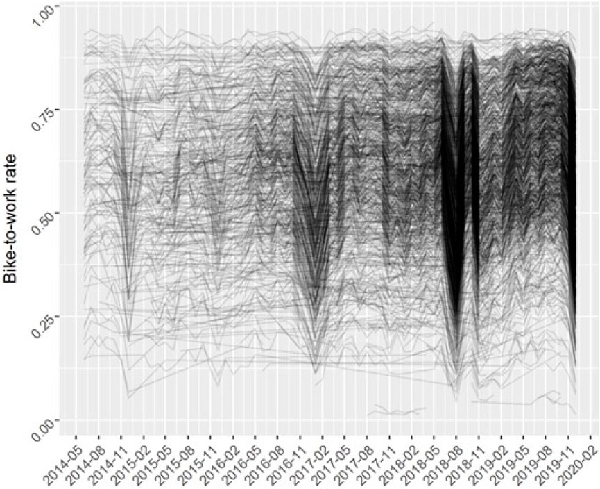
FIGURE 5. Model predicted person-level bike-to-work rate during the program.

We examine some of the effects of important variables through predictive plots (simulating predictions from our model holding variables at their means or reference category). The simulations have the benefit of showing the effect of variables on a meaningful scale (the bike-to-work rate). Just like Table 2 indicated, Figure 5 shows that the person level variation (the range of lines from top to bottom) is much larger than any predicted monthly level change for a given person. Although program compliance was set at 50–60 percent, many participants didn’t achieve that level of bicycling on average. However, nearly all participants biked to work 6 days a month or more (≥30%).

While winter months strongly reduced bike-commuting, commute distance has an even stronger reduction effect (Figure 6). Only the participants living within about 2.5 miles from work were on average bicycling 60% of the time during the program. At the same time, those with much longer commutes (up to 12.5 miles) were still predicted to bike commute above 50% on average. This finding suggests that bike and e-bike lending can work to encourage bike commuting at longer distances than are normally seen as “bikeable.”

FIGURE 6

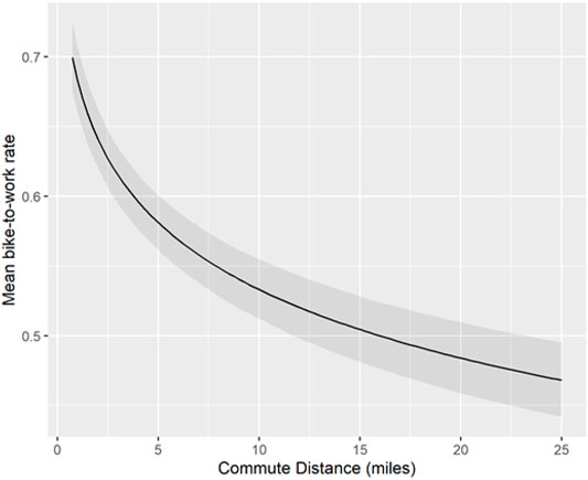
FIGURE 6. Model predicted mean bike-to-work rate of bike-lending participants by commute distance.

The difference between participants who chose a conventional bike instead of an e-bike was a surprise finding (Figure 7). On average, the conventional bike participants were predicted to bike to work at slightly greater rates compared to their e-bike counterparts without considering commute distance. We examined if the difference in bike commuting by bike type varied by commute distance but found no substantial moderating effect. Instead, after considering commute distance, the use of conventional and electric bikes our model predicted equivalent bike-to-work rates suggesting that e-bikes did not spur a lot of long-distance commuting (results not reported). While these results suggest conventional bikes may be a better choice for a lending program (especially considering their cost differences), we caution against the conclusion that conventional bikes alone could have achieved the same program demand that a paired conventional and electric bike lending program did. E-bikes have a large advantage for longer commutes and have been shown in many studies to increase use of bikes for transportation and car replacement (MacArthur et al., 2014; Fyhri and Fearnley, 2015). Many of the e-bike participants may never have participated had only a conventional bike been available. Without a controlled experiment where participants randomly get a conventional or electric bike (something no TDM program could feasibly tolerate), we cannot fully understand the effects of the different bike types.

FIGURE 7

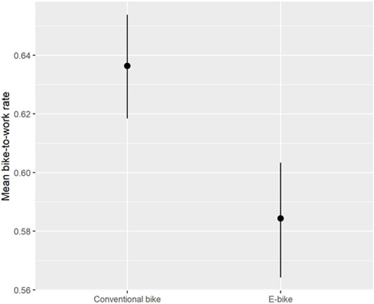
FIGURE 7. Model predicted mean bike-to-work rate of bike-lending participants by bike type.

Another somewhat surprising finding was the slight increase in bicycling during the program for participants who made multimodal journeys to work (Figure 8). We considered any bike journey to work multimodal if it included both the bike and either a form of public transit or GBus (we didn’t differentiate between GBus and public transit). However, making a multimodal commute with the bike is rare compared to a direct bike commute. It is only when people regularly make multimodal commutes that we observe a strong increase in bike commuting (Figure 8). Only conventional bike recipients were allowed to make multimodal commutes, so the multimodal effect is likely only applicable for conventional bicyclists.

FIGURE 8

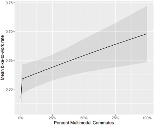
FIGURE 8. Model predicted mean bike-to-work rate of bike-lending participants by commute type.

Less surprising was the finding that more skilled bicyclists bike commuted at greater rates during the program (Figure 9). However, the fact that self-identified beginner bicyclists biked on average nearly 60% of the time suggests that bike lending programs do not have to only focus on advanced riders but can be used to target commuters with a wide variety of skill levels.

FIGURE 9

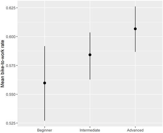
FIGURE 9. Model predicted mean bike-to-work rate of bike-lending participants by self-reported bicycling skill.

Finally, the model predicted effect of integrating Strava rides was negative (Figure 10). This either suggests that those who integrated Strava rides bike commuted less than their counterparts that chose to only self-report or only integrate some rides, or it indicates an over-reporting of bike commutes by self-reporters. With requirements to report bike commuting to maintain the loaned bike, there is more reason to think the latter explanation is more plausible, especially given that Strava app integration is intended to streamline reporting and reduce participant burden for those participants who already use Strava. The Strava effect is quite small for the participants who integrated Strava infrequently. But for those who used Strava for 100% of their trip reporting (about 50% of people who used Strava at all did so for 100% of their trips), the model predicts they biked about 30% less on average (an 18 percentage-point reduction). During the program, Strava integration was very rare (only 7% of person-months included at least one Strava trip), making this effect not that influential on program success if indeed Strava integration made it less likely for people to commute. However, if this effect is indicative of over-self-reporting of biking by non-Strava users, then the program effects we summarize below may be upward biased by a considerable amount.

FIGURE 10

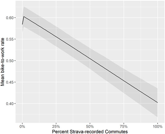
FIGURE 10. Model predicted mean bike-to-work rate of bike-lending participants by use of Strava app integration.

3.3 Predicted Program Effects

3.3.1 Bicycling to Work

We evaluated the effects of the program by predicting the change in bicycling between the before, during, and after phases using our model. Figure 11 shows the predicted mean bike-to-work rates as well as the person-level predictions. When predicting the program’s effect on bike commuting with only trip data, the results suggest an increase of more than 35 percentage points from before to during the program, and about 28 percentage points from before to after the program. This suggests the program caused substantial gains in bicycling during the program but saw a medium fraction of those gains lost after participants graduated from the program.

FIGURE 11

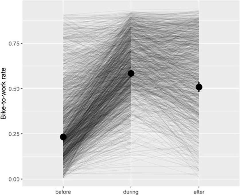
FIGURE 11. Model predicted bike-to-work rate of bike-lending participants by intervention phase from trip logs (before, during, after).

We also compared the same person-level predictions for the during and after phases with the survey data before participation (Figure 12). Because so many participants claimed to never bike to work before the program started, this comparison shows even larger bike commuting gains from the program. The benefit of this approach is that we have a unified general measure of bicycling right before the program. However, only 1,656 of the 2,712 participants (61%) reported a before measure of bike commute frequency making this approach likely systematically biased. Further, because we don’t have model estimates for the before survey data, we can’t predict before bike commuting for the missing responses like in the prior approach which means Figure 12 only includes a subset of participants (n = 1,656). Also, the applicants that did report bike commuting in the application could have been inclined to report less bicycling to work to increase their chances of getting a bike in the program. Nonetheless, using the survey as a baseline suggests that the program had a larger effect (close to 47 percentage point increase). The true program effect may be somewhere in between these estimates, although if the hypothesis that the Strava effect indicates systematic self-reporting bias the true effect could be roughly 30% less. In either analysis, including the potential over-reporting bias, the effects of the program on bicycling are clear. During program participation, bicycling to work is at its highest with more than 60% of commute trips by bike on average for participants. After participants graduate, they bike to work less than during the program, and the models predict bike commuting occurs greater than 50% of the time on average. Although we didn’t use the after-survey data in this analysis the modeled after effect is somewhat confirmed by the self-reported “rate of continuing to bike” in the after survey (76%) (i.e., the after survey indicates a 24% decline and the model estimate a 17% decline on average). This suggests that the program is leading to some sustained behavior change. However, because we cannot assess the reliability of the after data (see “Limitations” above), and because we suspect the after data may overestimate bicycling, we are less sure about the lasting effects of the program.

FIGURE 12

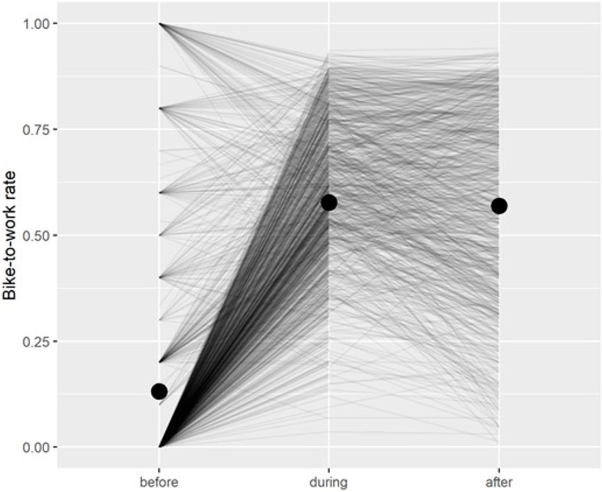
FIGURE 12. Model predicted bike-to-work rate of bike-lending participants by intervention phase from survey (before) and trip logs (during, after).

3.3.2 Single Occupancy Vehicle Commuting

We evaluated the reduction in SOV commuting from the program separately from bicycling to work to consider the fact that not all bike commutes substituted for SOV commutes. Because the reporting of non-bike commutes was not required for the program, only a small subset of participants (33%) reported SOV trips during the program. Additionally, SOV trips before and after the program are unreliable because so few participants reported them. We are not clear why these participants reported all their travel to campus (and not just bike travel). It may be that since the form allowed them to report all modes, they thought they had to as a part of the program requirements.

Figure 13 shows the expected effects of the program on reducing SOV commuting based on the before application survey and the model predicted SOV commuting rates during the program. Not surprisingly because the program targeted SOV commuters, the rate of SOV commuting dropped significantly during the program (a 55 percentage-point drop). Although there was some variation in the reduction in SOV commuting, the most common profile from this subset of participants was to go from an every-day SOV commuter to never SOV commuting. This suggests the program had a radical effect on commuting behavior for many people.

FIGURE 13

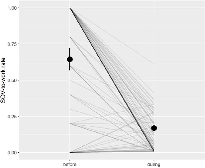
FIGURE 13. Model predicted SOV-to-work rate of bike-lending participants by intervention phase from survey (before) and trip logs (during).

When multiplying the predictive change in SOV commuting by commuting distance (assuming round trips by the same mode), the results suggest that for each commute day, participants reduced about 6 miles of SOV driving on average but showed great variation in daily SOV miles reduced (Figure 14). Furthermore, when applying the expected SOV reduction rates across all the participants during the program,⁴ we estimate the program reduced a total of nearly 400,000 SOV commute miles from inception in mid-2015 through the end of 2019 (Figure 15).

FIGURE 14

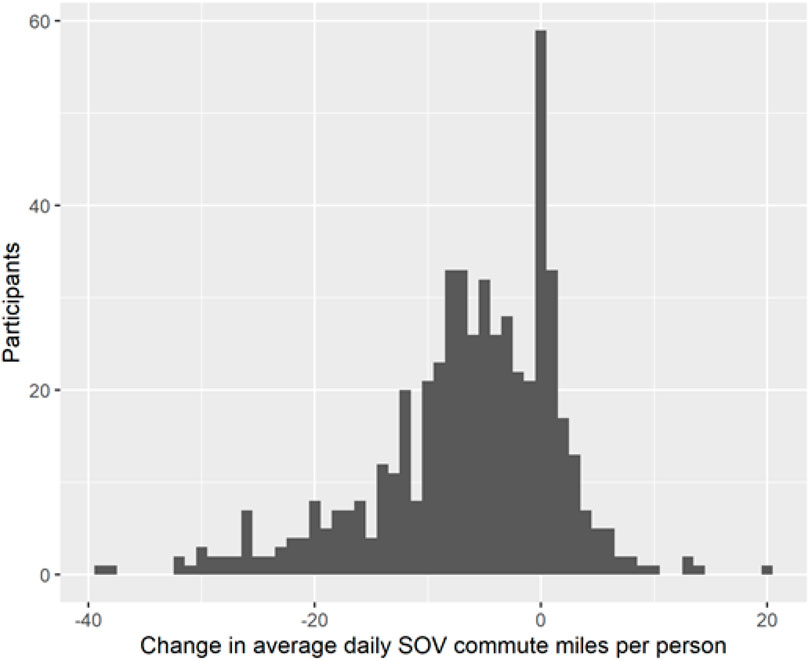
FIGURE 14. Implied daily SOV miles changes (during—before) per person based on model predicted SOV rates and self-reported commute distances.

FIGURE 15

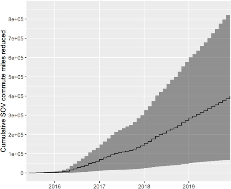
FIGURE 15. Estimated program-level cumulative monthly SOV miles reduced based on model predicted SOV rates and self-reported number of commute days and commute distance.

These estimates have several limitations. First, the model predicted SOV commute reduction exceeded the model prediction bike commute increases. This could mean that the program caused people to give up SOV commuting even on days they didn’t bike (e.g., by using transit, GBus, or carpooling). Alternatively, it could indicate a strong bias in the SOV reporting (before survey and/or during program trip logs). Second, because only a sub-sample of participants (33%) were used to model SOV rates, we are predicting out of sample for 67% of our data, such predictions may be biased, a reason why our estimated uncertainty is so large (Figure 15).

4 Discussion

The results from this analysis suggest that Google’s bike lending program substantially increased bicycling for program participants on the order of 1.7–2.3 days and 1.3–1.9 days of bike commuting per week on average during and after the program, respectively. In addition, nearly all the bicycling increases are likely attributed to reductions in SOV commuting. This resulted in approximately 15 miles of reduced SOV driving per week for an average participant. Even considering the limitations of this study, the magnitude of the behavior change from this program is likely to be large.

While the gains were large for both during and after the program, some participants discontinued bike commuting. There are many possible reasons for people returning to prior commute modes and some of them could be due to biased after-data reporting. Other program data indicates that not all participants used their incentive to purchase a bike (only 62% bought a bike after the program) suggesting even a six-month intervention has room for improvement. Also, in the select few respondents who took the exit survey (n = 746), nearly 22% of respondents said they do not plan to bike commute after the program. Some included reasons that suggest potential improvements to the program (e.g., limited shower facilities, e-bike too expensive) while other reasons will be more difficult for a TDM program to address (e.g., darkness and weather, road safety, need to shop on home-commute leg).

The decline in bike commuting after graduation suggests that a permanent lending program may be more efficacious. This approach would probably need to be paired with TDM managers following through with collecting the bikes if the participants are not meeting the reporting requirements or other disciplinary or encouragement strategies. However, the stated bike commute rate (60%) could still differ from the rate management uses to implement any action.

Future revisions to the program (or new programs) might also consider a wider variety of vehicle form factors. The Google lending program included two high-end commuter style e-bikes (Specialized Turbo and Giant Quick-e with estimates 25–60-mile e-range), and commuter road bikes, but nothing designed for carrying cargo/kids or folding on transit. Providing a greater variety of vehicles (including potentially e-scooters) could help increase program participation. Given the strong decline in bicycling during the wet season, vehicle forms that include some protection against rain would also likely be beneficial at increasing participation. Not surprisingly non-bike commuters saw the largest gains from the program. A continued focus on short to medium distance SOV commuters, and long distance SOV commuters with an option to travel by combined bike and transit will likely provide the most program benefits.

This evaluation is the first of its kind in the North American context. Bike lending could be an important component of TDM programs, especially with the rise in popularity of e-bikes and e-scooters. While bike lending is still rare, the Google case study shows that substantial behavior change is possible. Furthermore, this change is in the context of a common (by North American standards) suburban/urban heavily trafficked arterial street network. This suggests that the generalizability of these results to other large employment centers may be appropriate. Bicycling in and around Mountain View and Sunnyvale, CA, United States still requires a sense of confidence and willingness to put up with substantial traffic stress. For contexts that are more suited for bike commuting, bike lending may see even greater gains from more widespread adoption. Future research could focus on identifying the variation in program effects across program types and geographic contexts. Additionally, a deeper look at the costs and benefits of such programs are possible by leveraging the estimates of behavior change from this case study.

Data Availability Statement

The datasets presented in this article are not readily available because they are privately held by Google due to concerns about privacy. Requests to access the datasets should be directed to Lucy Noble, lucynoble@google.com.

Ethics Statement

Ethical review and approval was not required for the study on human participants in accordance with the local legislation and institutional requirements. Written informed consent for participation was not required for this study in accordance with the national legislation and the institutional requirements.

Author Contributions

The authors confirm contribution to the paper as follows: study conception and design: DF and LN; data collection: LN and TM; analysis and interpretation of results: DF and ZG; draft manuscript preparation: DF, ZG, LN, and TM. All authors reviewed the results and approved the final version of the manuscript.

Funding

This work was supported by Google and the Mineta Transportation Institute.

Conflict of Interest

Authors LN and TM are employed by Google. This study received funding from Google. The funder had the following involvement with the study: data collection, primary authors concerning the details of the TDM program, interpretation of some results where local context was needed, and editors of the manuscript to ensure omission of trade secrets. All authors declare no other competing interests.

Publisher’s Note

All claims expressed in this article are solely those of the authors and do not necessarily represent those of their affiliated organizations, or those of the publisher, the editors and the reviewers. Any product that may be evaluated in this article, or claim that may be made by its manufacturer, is not guaranteed or endorsed by the publisher.

Acknowledgments

We would like to thank UC Davis for supporting this research through computational resources, all the program participants who provided survey data, and the support staff at Google who helped organize the data.

Supplementary Material

The Supplementary Material for this article can be found online at: https://www.frontiersin.org/articles/10.3389/ffutr.2022.886760/full#supplementary-material

Footnotes

¹Results based on Google’s internal annual travel survey.

²Graduation occurred when a participant successfully completed a 6-month period of riding 60% of the time or more. Some participants graduated early to sync with on-campus bike sale events.

³The commuter benefits program at Google incentivizes employees who bike to work by giving them rewards (e.g., bicycling gear) in exchange for recording bike trip data.

⁴This calculation uses the SOV reduction from the sub-sample and applies it to the entire program.

References

Armstrong, E. P. (2010). Bike Sharing: A Randomized Study Evaluating the University of Oregon Bike Load Program. Eugene, OR: University of Oregon.

Google Scholar

Dill, J. (2009). Bicycling for Transportation and Health: the Role of Infrastructure. J. Public Health Pol. 30 (Suppl. 1), S95–S110. doi:10.1057/jphp.2008.56

CrossRef Full Text | Google Scholar

Fitch, D. T., Gao, Z., Noble, L., and Mac, T. (2022). Examining the Effects of a Bike and E-Bike Lending Program on Commuting Behavior. Mineta Transportation Institute. Available at: transweb.sjsu.edu/research/2051 (Accessed March 20, 2022).

Google Scholar

Fitch, D. T. (2019). Electric Assisted Bikes ( E-Bikes ) Show Promise in Getting People Out of Cars. Policy Brief. Davis: Institute of Transportation Studies, University of California. Available at: https://escholarship.org/uc/item/3mm040km (Accessed October 1, 2021).

Google Scholar

Fowler, S. L., Berrigan, D., and Pollack, K. M. (2017). Perceived Barriers to Bicycling in an Urban U.S. Environment. J. Transp. Health 6, 474–480. doi:10.1016/j.jth.2017.04.003

CrossRef Full Text | Google Scholar

Fyhri, A., and Beate Sundfør, H. (2020). Do people Who Buy E-Bikes Cycle More? Transp. Res. Part D Transp. Environ. 86, 102422. doi:10.1016/j.trd.2020.102422

CrossRef Full Text | Google Scholar

Fyhri, A., and Fearnley, N. (2015). Effects of E-Bikes on Bicycle Use and Mode Share. Transp. Res. Part D Transp. Environ. 36, 45–52. doi:10.1016/j.trd.2015.02.005

CrossRef Full Text | Google Scholar

Fyhri, A., Sundfør, H. B., and Weber, C. (2016). Effect of Subvention Program for Electric Bicycle in Oslo on Bicycle Use, Transport Distribution and CO₂ Emissions. TØI Rep., 114. https://www.toi.no/publications/effect-of-subvention-program-for-electric-bicycle-in-oslo-on-bicycle-use-transport-distribution-and-co2-emissions-article33886-29.html.

Google Scholar

Handy, S. L., Xing, Y., and Buehler, T. J. (2010). Factors Associated with Bicycle Ownership and Use: a Study of Six Small U.S. Cities. Transportation 37, 967–985. doi:10.1007/s11116-010-9269-x

CrossRef Full Text | Google Scholar

Haubold, H. (2016). Electromobility for All: Financial Incentives for E-Cycling. Brussels, Belgium: European Cyclists’ Federation.

Google Scholar

Heinen, E., van Wee, B., and Maat, K. (2010). Commuting by Bicycle: an Overview of the Literature. Transp. Rev. 30, 59–96. doi:10.1080/01441640903187001

CrossRef Full Text | Google Scholar

Lally, P., Van Jaarsveld, C. H. M., Potts, H. W. W., and Wardle, J. (2010). How Are Habits Formed: Modelling Habit Formation in the Real World. Eur. J. Soc. Psychol. 40, 998–1009. doi:10.1002/ejsp10.1002/ejsp.674

CrossRef Full Text | Google Scholar

Lamy, V. (2001). Electric Bike 2000. Montreal, QC: Transportation Development Centre, 46.

Google Scholar

Litman, T. (2021). Evaluating Active Transport Benefits and Costs: Guide to Valuing Walking and Cycling Improvements and Encouragement Programs. Victoria Transport Policy Institute. Available at: https://www.vtpi.org/nmt-tdm.pdf (Accessed January 20, 2022).

Google Scholar

MacArthur, J., Kobel, N., Dill, J., and Mummuni, Z. (2016). “Evaluation of an Electric Bike Pilot Project at Three Employment Campuses in Portland, Oregon,” in Transportation Research Board 95th Annual Meeting, 19. doi:10.15760/trec.158

CrossRef Full Text | Google Scholar

MacArthur, J., Dill, J., and Person, M. (2014). Electric Bikes in North America: Results of an Online Surveya. Transp. Res. Rec. 2468, 123–130. doi:10.3141/2468-14

CrossRef Full Text | Google Scholar

MacArthur, J., Harpool, M., Scheppke, D., and Cheery, C. R. (2018). A North American Survey of Electric Bicycle Owners. Portland, OR: National Institute for Transportation and Communities (NITC). NITC-RR-1041.

CrossRef Full Text | Google Scholar

Nozick, L. K., Borderas, H., and Meyburg, A. H. (1998). Evaluation of Travel Demand Measures and Programs: A Data Envelopment Analysis Approach. Transp. Res. Part A Policy Pract. 32, 331–343. doi:10.1016/S0965-8564(97)00043-8

CrossRef Full Text | Google Scholar

Pucher, J., Dill, J., and Handy, S. (2010). Infrastructure, Programs, and Policies to Increase Bicycling: An International Review. Prev. Med. 50 (Suppl 1 ), S106–S125. doi:10.1016/j.ypmed.2009.07.028

PubMed Abstract | CrossRef Full Text | Google Scholar

Ramezani, S., Hasanzadeh, K., Rinne, T., Kajosaari, A., and Kyttä, M. (2021). Residential Relocation and Travel Behavior Change: Investigating the Effects of Changes in the Built Environment, Activity Space Dispersion, Car and Bike Ownership, and Travel Attitudes. Transp. Res. Part A Policy Pract. 147, 28–48. doi:10.1016/j.tra.2021.02.016

CrossRef Full Text | Google Scholar

Shoup, D. C. (1997a). Evaluating the Effects of Cashing Out Employer-Paid Parking: Eight Case Studies. Transp. Policy 4, 201–216. doi:10.1016/s0967-070x(97)00019-x

CrossRef Full Text | Google Scholar

Shoup, D. C. (1997b). The High Cost of Free Parking. J. Plan. Educ. Res. 17, 3–20. doi:10.1177/0739456X9701700102

CrossRef Full Text | Google Scholar

Sundfør, H. B., and Fyhri, A. (2017). A Push for Public Health: The Effect of E-Bikes on Physical Activity Levels. BMC Public Health 17, 1–12. doi:10.1186/s12889-017-4817-3

PubMed Abstract | CrossRef Full Text | Google Scholar

Xing, Y., Handy, S. L., and Mokhtarian, P. L. (2010). Factors Associated with Proportions and Miles of Bicycling for Transportation and Recreation in Six Small US Cities. Transp. Res. Part D Transp. Environ. 15, 73–81. doi:10.1016/j.trd.2009.09.004

CrossRef Full Text | Google Scholar

Zhu, C., Yue, J. S., Mandayam, C. V., Merugu, D., Abadi, H. K., and Prabhakar, B. (2015). “Reducing Road Congestion Through Incentives: A Case Study,” in Transportation Research Board 94th Annual Meeting, Washington, DC, January 11–15, 2008.

Google Scholar