 Davoud Alahvirdi
 Elio Tuci
- Robotics Lab, Computer Science Faculty, University of Namur, Namur, Belgium
Traffic monitoring is a critical aspect of urban infrastructure management. With the advancement of technologies, traditional surveillance methods based on fixed sensor network systems could be potentially replaced by adaptive and easily redeployable systems, such as those based on drones. This paper wishes to contribute to the development of drones-based traffic monitoring and management systems by describing and evaluating a simulated swarm of drones monitoring traffic and communicating traffic data to adaptive traffic lights which adapt their green light duration to the current volume of traffic using the SPSA optimisation algorithm. A cell transition model (CTM) is used to simulate the behaviour, flow, and interactions of vehicles within a road network larger than most of networks used in similar studies. Evaluation tests compare the effectiveness of adaptive traffic unit with data generated by drones with a system of fixed duration signal traffic lights, and with an adaptive traffic unit with data generated by fixed cameras. The results shows that the optimised traffic lights system with data generated by drones is more effective than both the fixed signalling duration and the optimised system with data generated by fixed cameras in resolving traffic congestion due to a high volume of cars entering the road network. Further post-evaluation tests illustrate the limits of the adaptive traffic unit system with data generated by drones under a progressively higher volume of traffic entering the road network. We conclude the paper by discussing the current limitations of our model and by pointing to the most interesting directions for future work.
1 Introduction
Unmanned aerial vehicles (UAVs), commonly known as drones, have emerged as a transformative force in various fields such as precision agriculture, wildlife conservation, delivery, logistics, and etc. The ability for vertical take-off and landing within limited spaces and their impressive speed and agility have induced researchers to exploit drones in a wide range of tasks in particular in those requiring surveillance and data collection such as traffic monitoring and management tasks. The exponential rise in the number of vehicles in the road networks have largely contributed to the emergence of frequent traffic congestion problems as well as of problems related to air and sound pollution in urban areas (Anjum et al., 2021; Goetz, 2019). Sensor-network based technology, exploiting fixed camera Radivojević et al. (2021), ultrasonic sensors Tan et al. (2020), and RFID—Radio Frequency Identification—reader Atta et al. (2020), have made possible to address the negative effects of traffic on quality of life and on wellbeing of citizens with effective strategies to monitor, and possibly alleviate, vehicle congestion on urban roads and motorways (Fadda et al., 2022; Appiah et al., 2020; Tasgaonkar et al., 2020). For example, in Neelakandan et al. (2021); Zhang et al. (2020); Kuang et al. (2021); Desmira et al. (2022), a combination of fixed sensor-networks and different AI-based algorithms are presented to manage traffic by regulating traffic-light timing. These systems has been proved quite effective in reducing the average waiting time of vehicles in the road networks. Nevertheless, sensor-network based technology suffers from several limitations, primarily determined by the relatively high cost of maintenance operations such as sensor calibration, as well as from the fact that the technology is not particularly suitable to be deployed in very large areas (Narisetty et al., 2021; Ravish and Swamy, 2021). Furthermore, this technology, being anchored to the ground, completely lacks the flexibility and adaptability required to be easily and continuously redeployed in different areas to track the development of vehicle traffic on large road networks. To overcome the limitations of fixed sensor-networks, drones have emerged as a costs effective technology, that has the advantage to be easily deployed in different and potentially large urban zones to carry out tasks related to road safety, motorway infrastructure management, and traffic monitoring (Gohari et al., 2022; Dilshad et al., 2020; Bisio et al., 2022).
The scientific literature on single or multiple UAVs systems employed for urban activities, including traffic monitoring, is already quite vast. A possible way to sort this large body of research is by classifying these works in those that we referred to as “general” and those that we referred to as “specific.” In the “general” category we include those research works that focus on challenges in urban air mobility common to multiple applications. Many of these studies focus on problem related to the generation of trajectories for UAVs required to fly at low altitudes in cluttered scenarios, characterised by natural and man-made obstacles. In Causa and Fasano (2021), the authors illustrate a obstacle-free path planning algorithm for multi UAVs based on the multi-step strategies that include automated definition of GNSS-challenging volumes based on a georeferenced three-dimensional environment model, derivation of candidate obstacle-free paths between waypoints, waypoint assignment and definition of time-tagged trajectories to cope with path planning issues in low altitude environment. In Nguyen et al. (2021), the authors developed a drones-based traffic monitoring system in which the drones fly on trajectories that are defined using GPS points. The scientific contribution of this work is in demonstrating that GPS trajectories are more effective than map based routes. In Elloumi et al. (2018), an innovative road traffic monitoring system is characterised by multiple drones generating adaptive flying trajectories, which are based on the tracking of moving points within the UAV field of view. Other papers propose algorithms that allow drones to minimise travel time in missions that require drones to visit multiple sites. For example, in Christodoulou and Kolios (2020) and Garcia-Aunon et al. (2019), the authors describe methods to allow drones to minimise travel time based on point of interests (POIs) and genetic algorithm, respectively.
In the “specific” category, we include those research works that focus on issues related to specific applications, with a main focus on research works in which air mobility is applied to the development of traffic monitoring and management systems. In Roldán-Gómez et al. (2022), a swarm of simulated drones is deployed to monitor traffic by counting the number of vehicles in a virtual city called swarm city and to share this data with a ground station unit. In these investigations, the shared data were used to generate maps represented in a virtual reality interface. In Hanzla et al. (2024), the authors introduce a smart traffic monitoring solution to address challenges in vehicle detection and tracking, by segmenting images taken by drones using deep learning technology (i.e., YOLOv5) and Kalman Filter based algorithms. In Zhu et al. (2018), the authors also exploited deep neural network algorithms to process videos recorded by a swarm of drones in order to detect and localise vehicles. Several drones-based traffic monitoring systems used a centralised approach in which the information gathered by drones is transferred to a human-operated central unit that processes the data and makes decisions concerning the management of traffic congestion. In studies that adopt this approach, the research focuses on issues related to the communication between drones and the central decision unit (Elloumi et al., 2018). Human errors, delays in response time, and difficulty in handling emergency conditions are the main drawbacks of the centralised traffic management systems (Yadav et al., 2021). To overcome these challenges, decentralised and adaptive traffic stations, exploiting machine learning methods (such as reinforcement learning algorithms), have been investigated. Some of these decentralised traffic systems regulate the traffic light duration as in Saleem et al. (2022); Abdoos and Bazzan (2021). In Chow et al. (2020), centralised and decentralised optimal control strategies are compared based on the Hamilton-Jacobi formulation of the kinematic traffic model. The optimal methodologies are applied to a set of test scenarios constructed from a real road network in central London (UK). In Yao et al. (2022), the authors illustrate an optimised traffic signal controller based on SPSA algorithm for a mixed traffic flow composed of automated and human driven vehicles by using CTM traffic model. The optimised control effectively reduces the range and the dissipation time of traffic congestion in comparison with fixed timing control. Mixed traffic flow is characterized by connected automated vehicles (CAVs), connected vehicles (CVs), and regular vehicles (RVs). In Qin et al. (2024), an analyticalmixed traffic capacity model for minor roads in an intersection is proposed to estimates their passing probabilities between CAV-led and CV/RV-led platoons.
In most of the applications within the framework of urban air mobility, an advanced and reliable communication protocols is required to exchange data between drones and ground stations. Due to the limited resources available to run highly secure algorithms on board, authors in Hassija et al. (2021) investigated the effectiveness of communication methods such as blockchain, software defined networks (SDN), and machine learning to neutralise the effects of attacks such as man-in-the-middle or de-authentication. In Ivancic et al. (2019) and Guirado et al. (2021), the authors present internet-based communication protocols named 4G LTE method for real-time transfer of video and images between air traffic management units and small unmanned air vehicles to address communication challenges. In Aloqaily et al. (2022), a UAV-supported vehicular network is implemented where drones and traffic units are considered as separate nodes that communicate with each other through the 5G connection and ad hoc links. To make communication more secure against cybersecurity attacks, a novel distributed way for drone-to-drone communication is illustrated in (Kumar et al., 2022). This secure method comes with some drawbacks such as limited bandwidth, spectrum constraints, and the requirement of the use of a large quantity of drones to cover a vast city map.
As in Yao et al. (2022) mentioned above, the research work described in this paper focuses on a system that manages traffic using drones. In particular, we illustrate and evaluate a decentralised multiple UAVs based system that by patrolling urban network, count cars on different roads and communicate this information to traffic lights signals. The signalling system uses this information to adjust signalling time using an optimisation method in order to reduce any eventual congestion. We consider a road network that consists of three connected two-way two-lanes cross intersections, we model traffic using CTM traffic model, and we defined fixed meeting points where the drones can share data with traffic light signals at regular intervals. We show that, when a high concentration of traffic is detected by drones in any part of the network, the traffic light unit concerned with the congestion, made aware of the problem by drones, resolves the congestion (i.e., it reduces the volume of traffic) by using the optimisation algorithm to adjust the green traffic light duration. In order to provide a term of comparison for the performance of the drones-based system, we also evaluate in identical conditions an alternative sensor-network based system in which information about traffic is generated and transferred to traffic lights by fixed camera. The results show that the drones-based system is more effective than the sensor-network based system. The original contribution of this study is in demonstrating the effectiveness of the above described drones-based traffic management system in a more complex scenario than the one employed in other similar studies such as in (Yao et al., 2022). We target a more extended road network than those described in the literature for similar drone-based technology, with a greater number of interconnected intersections and a realistic traffic signalling system, where traffic units control and optimise the flow of forward/right turn, and left turn traffic. Moreover, we evaluate the robustness of the mentioned traffic management system in a larger set of traffic flow input conditions in comparison with (Yao et al., 2022).
The remaining of this paper is structured as follows: the general methodological approach is described in Section 2, with Section 2.1 and 2.2 illustrating the whole of the city layout model and the traffic light phases, respectively; Section 2.3 illustrating the traffic model; the route planning for the navigation of drones is described in Section 2.4; the traffic lights optimisation algorithm is illustrated in Section 2.5. Simulation results are shown in Section 3, and finally conclusions are drawn in Section 4.
2 Methodology
This Section describes the methods used to develop the simulation modelling an urban scenario with a swarm of drones carrying out the traffic monitoring and management task. As illustrated in Figure 1, the simulation model is made of the following three layers: i) the city-layer, ii) the drone-layer, and iii) the traffic-layer. The city-layer includes the road map, the traffic model, and the routes the drones follow during inspection. The road map describes an urban environment, with a geographically realistic representation of road networks with lanes, intersection geometries, and relevant infrastructure such as traffic signals. The traffic is implemented using CTM which is an inflow-outflow mathematical formulation used to simulate and analyse the flow of traffic within the road network. The routes refer to the trajectories that drones follow to monitor the traffic. Each drone has two possible routes. The switching between routes by drones is triggered by specific conditions concerning the level of traffic within the route currently monitored. Within each route, there are meeting points; that is, points in which drones and traffic signals are sufficiently close (
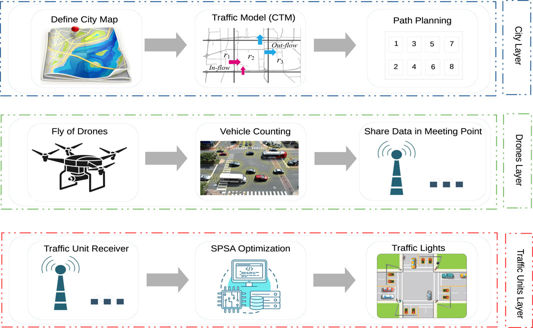
Figure 1. The three layered structure of the traffic simulator: the City Layer on top, the Drone Layer in the middle, and Traffic Unit layer at the bottom.
2.1 The road network
The road network is made of three two-way two-lanes cross intersections (four legs) connected as illustrated in Figure 2. Each leg has two entry and two exit points to the intersection. The entry points are one for vehicles moving forward and turning right, and the other entry for vehicles turning left. The exit points are one for receiving vehicles travelling forward and for those leaving the intersection with a right turn, and the other exit for vehicles leaving the intersection with a left turn. In the road network, there are a total of 48 entry/exit points to intersections, which we refer to as
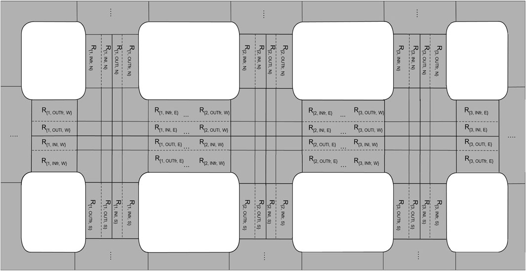
Figure 2. The road network made of three two-way two-lanes cross intersections. The notation refers to the entry and exit points to the intersections.
2.2 The three sets of traffic lights
Three sets of traffic signals control the traffic at each intersection. Each traffic light has a cycle characterised by four phases, as illustrated in Figure 3. In order to implement the four phases, each set is made of four traffic signals, with each traffic signal made of two subsets of two lights (i.e., one red and one green light). The two-light subset referred to as
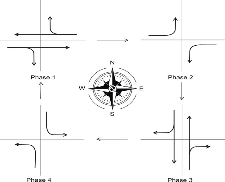
Figure 3. The phases of the traffic lights.
Note that, we do not include the yellow light, since, being a fixed duration signal, generally overlapping with the green—and sometime with the red—light, we consider that it has only marginal and potentially negligible effects on the emergence and dissipation of traffic congestion. Nevertheless, at this stage of our exploration, the elimination of yellow light considerably simplifies our model.
2.3 The traffic model
We use the cell transition model (CTM) to simulate the vehicles’ movement on the road network (Yao et al., 2022). CTM is a cellular automaton traffic model that is widely used in the literature since it offers several advantages in terms of definition and analysis of traffic dynamics based on cells’ input and output flow. The model represents the road network as a series of discrete cells, in which the length of each cell is calculated based on the distance travelled by free-flow traffic in one evaluation time step. Each cell corresponds to a segment of the road. The non-continuous (in time and space) flow of traffic between adjacent cells of the CTM is shown in Figure 4a, where for cell
where,
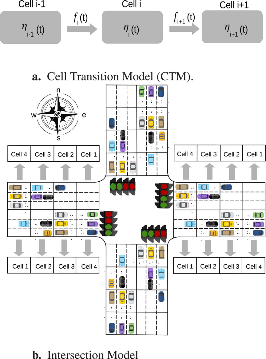
Figure 4. (a) Drawing showing the cells of the Cell Transition Model (CTM) in a portion of the road network. (b) Diagram showing the flow of traffic between adjacent cells in the CTM.
The following requirements must be met for the traffic flow:
with
with
Based on the Equations 6–8 can be simplified as follows.
More detailed information about CTM model can be found in (Yao et al., 2022). Based on Equation 9, CTM is suitable for capturing fundamental traffic dynamics. However, it has limitations in representing more complex behaviours, especially in urban environments with dynamic conditions, such as: frequent lane changes, pedestrian interactions, heterogeneous vehicle movements and/or driving behaviour, etc. These phenomena can be more effectively captured by microscopic traffic flow simulation software, which we will use in future works.
2.4 Route planning for drones
Four drones monitor and manage the road traffic on the entire road network by flying along predefined paths. Each drone is assigned to a specific portion of the road network which can be monitored by following two distinctive routes. In each route, only the roads that are part of the monitored road network are considered by the drones, as shown in Figure 5. Each drone keeps on flying on the same route unless specific traffic conditions are met, following which the done swap route (see Section 2.5 for details on the conditions triggering the route swapping). In the current implementation, drone coordination is managed by the traffic unit at the meeting point, which assigns tasks and ensures each drone collects relevant data. While this centralized approach is sufficient for the three-intersection network, we acknowledge that larger networks would require more sophisticated, possibly decentralized, coordination strategies. The camera is oriented in a nadir (downward-facing) position of the drones with a fixed angle of view. In the cellular model, to ensure complete coverage of a single cell, the drones should fly at a specific flight altitude
where
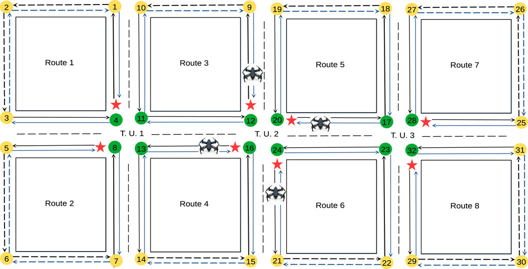
Figure 5. Routes of four traffic-monitoring drones, with continuous lines for monitored roads and dashed lines for unmonitored roads.
2.5 Traffic signal optimisation
The simultaneous perturbation stochastic approximation (SPSA) algorithm is used to set the conditions to minimise the traffic and to avoid traffic congestion on the road network. The information about the current traffic conditions (i.e., the number of cars in each of the monitored cells) are communicated at regular intervals by the drones to the closest traffic lights every time they reach a meeting point. The traffic light runs the SPSA algorithm to adjust the duration of the green light with the objective of reducing traffic while taking into account constraints determined by the intersection signal timing control and the flow transmission relationship between cells. The SPSA algorithm is a powerful heuristic method that gradually approximates the optimal solution by iteratively estimating the gradient information of the objective function. The algorithm employs two estimated values of the objective function, which is independent of the dimension of the optimisation problem. The feature of perturbing each variable in both positive and negative directions allows the algorithm to estimate the gradient of the objective function more robustly. After perturbing the parameters, SPSA observes the corresponding changes in the objective function. By averaging these perturbations, SPSA computes an approximation of the gradient, adapting its steps based on this approximation to iteratively refine the solution. This adaptability allows SPSA to handle noisy objective functions and to converge efficiently, even in the presence of uncertainties or fluctuations. In our road traffic scenario, the objective function tries to minimise the overall delay
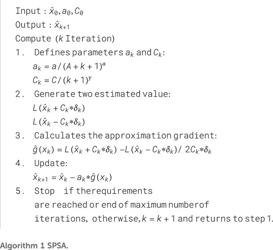
Algorithm 1. SPSA.
Where,
The objective function aims to minimise the time vehicles spend waiting or moving slowly in the total length of each lane by increasing the number of cars leaving each lane. The delay of a single cell is described as the difference between the number of vehicles in cell i at time t (see Equation 1 and the number of departing vehicles as in Figure 4a.
where
Y = 4 is the number of CTM sub-cells for each road network. Finally, the objective function is achieved based on Equation 12 as:
From Equation 13, it can be concluded that when
2.6 Constraints
Note that, several assumptions are made to simplify the simulation process and allow for a more detailed investigation into specific aspects of the study. As mentioned above, the fixed length yellow light is not considered. The sum of the green light duration for all traffic lights at an intersection
The travel time required by drones to change routes is not considered. By neglecting the travel time for route changes, the simulation focuses more narrowly on specific aspects of drone behaviour, such as counting vehicles and the communication with the traffic unit layer. Finally, we define
3 Results
In this Section, we show the results of a series of tests aimed at evaluating the efficiency and robustness of the traffic monitoring and management system based on the adjustment of the green light duration of traffic signals using the SPSA optimisation control. In the following, we refer to this as the adaptive green light duration condition. In particular, we run three types of tests: i) test A, a test in which a fixed green light duration condition is compared with the adaptive green light duration with traffic data generated by drones monitoring the road network as illustrated in Figure 2. ii) test B, a test in which the adaptive green light duration condition with data generated by a set of fixed camera system is compared with the adaptive green light duration with traffic data generated by drones monitoring the road network; iii) test C, a test in which the adaptive green light duration with data generated by drones monitoring the road network is subjected to a progressively higher volume of traffic entering the road network. In all the three types of tests, the traffic is simulated with the CTM model. The length of each cell of the CTM model is set to 50 m, and the maximum capacity of each cell for the
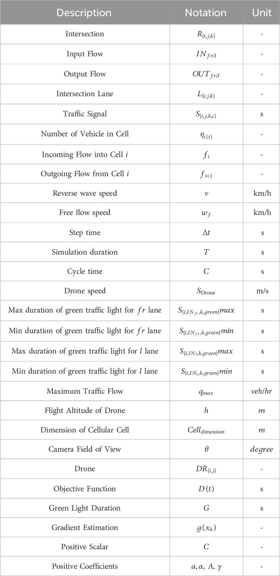
Table 1. Table of symbols.
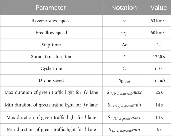
Table 2. Values of the simulation parameters used during the evaluation tests.
3.1 Test A: comparison between fixed and adaptive green light duration conditions
This is the test in which we compare the development of traffic in a condition in which traffic lights operate with a fixed signalling duration with the development of traffic in a condition in which traffic lights adjust the green light duration with the SPSA optimisation algorithm using data generated dy drones. We assess the system’s performance using a constant input flow with 20 vehicles per minute entering
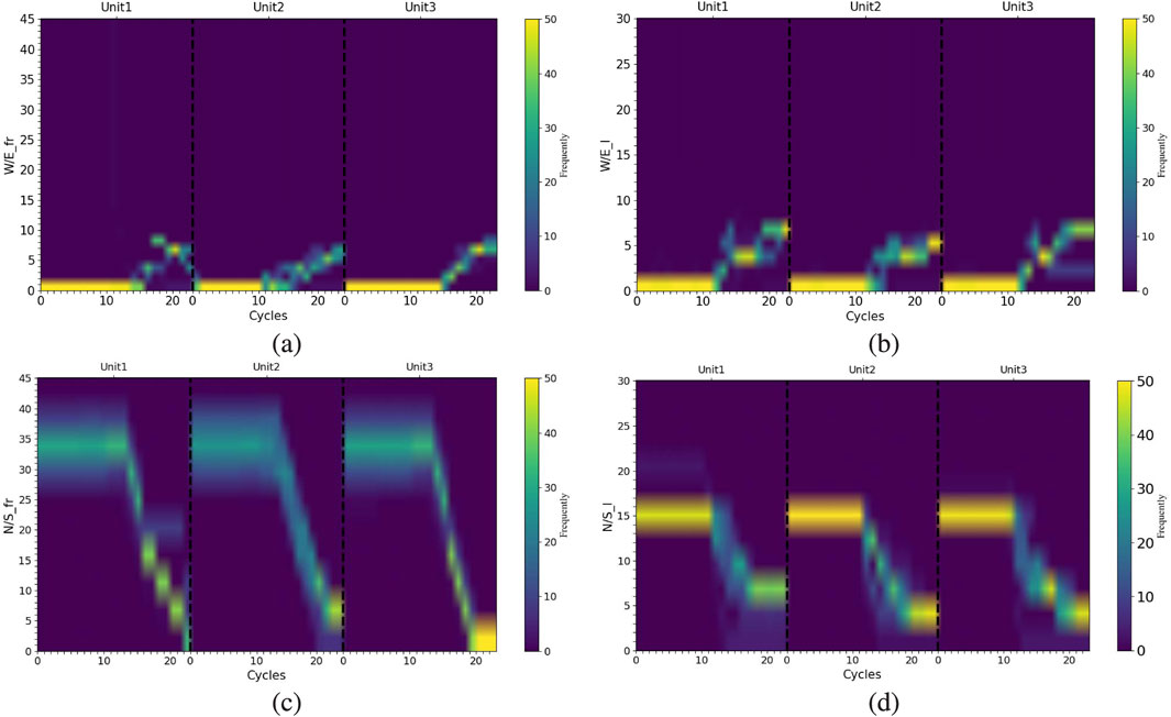
Figure 6. Graphs showing the evolution of traffic monitored by showing the frequency of the different values of (a)
The results of our evaluation tests are shown in Figure 6, where Figures 6a,b refer to the evolution of traffic on the west/east direction, and Figures 6c,d refer to the evolution of traffic on the north/south direction at each intersection
From cycle 10, to the end of the simulation time (i.e., cycle 22), we see that the traffic evolves in a radically different way in response to the activation of the adaptive traffic unit, which by receiving data on traffic from drones, it increases the duration of the green light for phase 3 (i.e.,
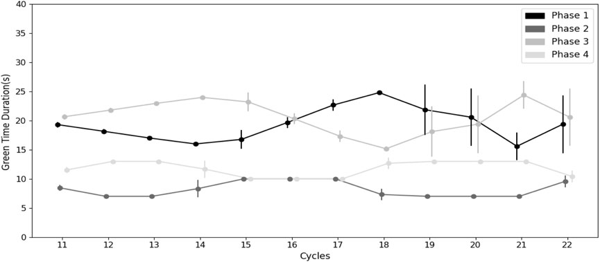
Figure 7. Graph showing the mean value and standard deviation, over 50 simulation runs, of the optimised duration of the green signals of traffic light 2, for phase 1 (black line, corresponding to signals
3.2 Test B: comparison between camera generated and drones generated traffic data
To provide a comparative framework that helps to assess the performance of the drones-based system, we have compared the development of traffic in a condition in which traffic lights adjust the green light duration with the SPSA optimisation algorithm using data generated by a fixed set of cameras, with the development of traffic in a condition in which traffic lights adjust the green light duration with the SPSA optimisation algorithm using data generated by drones. In the fixed camera condition, we assume that each intersection is equipped with four stationary cameras each oriented toward a different cardinal point. Each camera has a field of view of 50 m sufficient to correctly count cars in the last cell (i.e., cell 4, the cell in the immediate proximity of the traffic light) of the viewed lanes. Thus, contrary to the drones-based system which delivers data related to the number of cars along the entire flying path, cameras can only generate and deliver accurate data related to the cells closest to the traffic lights. Note that our aim is to model a generic camera-based system that we assume with a limited view of the roads compared to the drones-based system. This assumption follows from general considerations on practical aspects related to the specifications of cameras used for this type of application, as well as on other aspects such as the height at which cameras are usually mounted. This limitation may not necessarily apply to all camera-based systems for traffic monitoring. This issue will be discussed in Section 4.
In the tests, the initial traffic conditions and the frequency of cars entering into the road network as well as any parameters of the system remain unchanged from previous set of tests illustrated in Section 3.1. Moreover, as in tests A, we have executed 50 differently seeded simulation runs, differing in the initial distributions of the 20 vehicles among the cells of the
The results of our evaluation tests are shown in Figure 8, where Figures 8a,b refer to the evolution of traffic on the west/east direction, and Figures 8c,d refer to the evolution of traffic on the north/south direction at each intersection
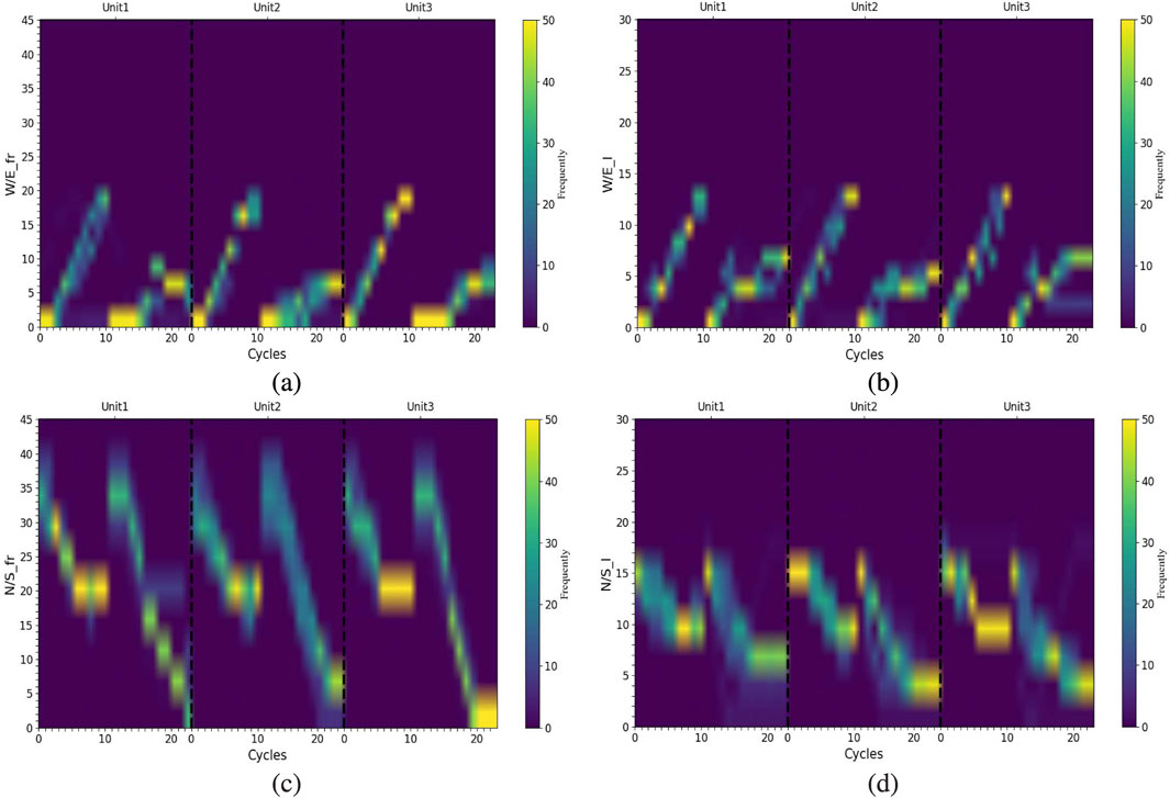
Figure 8. Graphs showing the evolution of traffic monitored by showing the frequency of the different values of (a)
The traffic develops in a similar way on the
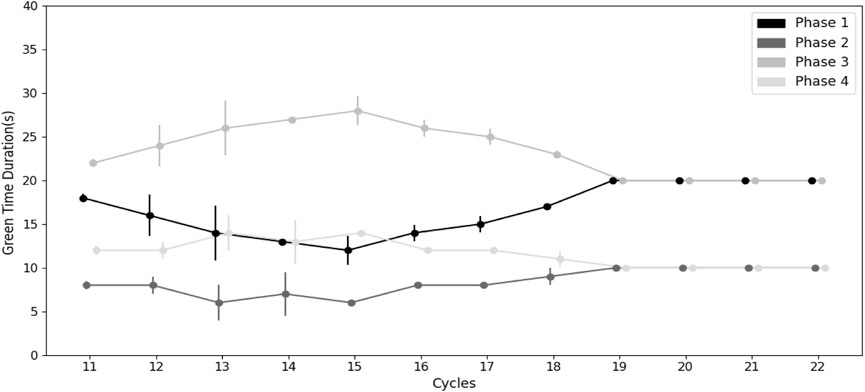
Figure 9. Graph showing the mean value and standard deviation, over 50 simulation runs, of the optimised duration of the green signals of traffic light 2, for phase 1 (black line, corresponding to signals
3.3 Test C: adaptive green light duration on a progressively higher volume of traffic
In a further set of post-evaluation tests, we have evaluated the robustness of the SPSA optimisation algorithm to cope with a progressively higher volume of vehicles entering into the road network. In particular, we have considered different scenarios, in which the input flow of vehicles at intersection
Figure 10 shows the results of the robustness test by illustrating, for each scenario, and for each traffic light cycle, the frequency occurrence for
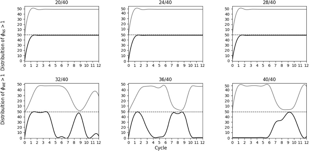
Figure 10. Graph showing the frequency of occurrence for
4 Conclusion
This paper describes and evaluates a simulated drones-based system for traffic surveillance and management. In our model, the drones patrol different parts of the road network by counting cars forming the urban traffic. The number of cars are communicated by drones to traffic lights, which, by running the SPSA optimisation algorithm, adapt the green light duration to resolve any eventual congestion. In our study, the road network is composed of eight roads and three signalled intersections. The roads are patrolled by four drones deployed to monitor the road traffic by flying along predefined paths. We have evaluated the drones-based system by monitoring the traffic on the road network under two different conditions: with fixed (predefined green light duration) and with adaptive (i.e., SPSA determined) green light duration. We have also compared the drones-based system with a sensor-network based surveillance system made of cameras placed at the road intersections pointing to the four different legs of each signalled intersection. Compared to the drones-based system, the sensor-network based system is conceived limited in its capacity to count cars, since the cameras precisely count cars only in the proximity of traffic lights1. The evaluations are run under specific initial traffic conditions and predefined number of cars entering the road network with more cars entering the N/S than the W/E lanes. We show that with the fixed light duration, the number of cars on the N/S lanes (i.e., the most congested lanes) remains constant with cars jammed entire the roads at each intersection. With the adaptive green light duration, the number of cars on the N/S lanes tends to progressively decrease until no cars jammed entire the roads at each intersection. This is the result of the effects of the SPSA optimisation algorithm which increases the green light duration for the N/S lanes in response to data generated by drones. Since the increase of the green light duration for the N/S lanes corresponds to a decrease of the green light duration for the W/E lanes, the number of cars on these lanes tends to slightly increase. In summary, we have shown that, contrary to the fixed green light duration condition, the adaptive green light duration condition is effective in resolving traffic congestion determined by the flux of incoming cars into the network. The comparison between the drones-based and the sensor-network based system demonstrates that the drones-based system is more effective than the sensor-network based system in resolving traffic congestion.
We acknowledge that, as a first model evaluating a specific urban traffic monitoring and management system based on drones counting cars and optimised system adjusting green light duration, several simplification have been made. On top of those already discussed in 2.6, in our model we assume that four drones are sufficient to exhaustively patrol the entire road network. This may not necessarily be the case especially in large cities, where a too high number of drones may be required to exhaustively patrol the road network. In this study, we do not look at phenomena related to the ratio between number of drones and extension of the road network. Nevertheless, these issues may be of absolute relevance for a system where traffic is monitored by drones and managed by an optimisation algorithm working on drones generated data. If the road network is too large to be exhaustively patrolled by the available drones, several issues emerge related to the capability of drones: i) to position themselves in order to maximise traffic observability; ii) to redeploy themselves in response to changes in the traffic conditions; iii) to manage energy efficiently to maximise battery-life and operation time. Moreover, in this study we do not consider the possibility of replacing drones once their batteries are exhausted to monitor and manage traffic for a period of time longer than the average drone battery life. This can be achieved by creating one or more charging points where drones can return and autonomously recharge their batteries. Given that drones have the capacity to take off and to land vertically, charging points could be created in urban environment by exploiting already existing facilities, such as flat roofs of sufficiently high buildings. We acknowledge that a time complexity/computational cost analysis of the drone-based system is required to correctly evaluate and effectively tackle some of the above mentioned issues which significantly impact on the possibility to deploy this system in real-world conditions. We leave this analysis to future work.
Another aspects which we did not consider is related to the synchronisation of traffic lights behaviour. Clearly, a system in which traffic lights located on the same road behave in a synchronous way may be potentially more effective in resolving traffic congestion than a system like the one we modelled in which traffic lights do not interact. The synchronisation or any other form of coordination between traffic lights can not be achieved by the system we described in this paper, since there is no means for traffic lights to interact and coordinate. This is another important issue that we intend to explore in future work.
In this study we have compared the drones-based system with a sensor-network based system intentionally conceived limited in its capacity to monitor the road network. Future work may focus on progressively reducing the limitations imposed to the sensor-network based system to quantitatively evaluate the extend to which observability related issues influence the effectiveness of the algorithms adapting the green light duration. This will also be the subject of future work. Finally, it is worth to consider that the use of drones in scenarios like the one illustrated in this paper may require modifications to the current regulations that governed drones operations in terms of both operational and technical requirements.
Data availability statement
The raw data supporting the conclusions of this article will be made available by the authors, without undue reservation.
Author contributions
DA: Writing – review and editing, Writing – original draft. ET: Writing – review and editing, Writing – original draft.
Funding
The author(s) declare that financial support was received for the research and/or publication of this article. This work was supported by University of Namur.
Acknowledgments
We would like to express our deepest gratitude to Alexandre Mauroy and Julien Pietquin, for their invaluable guidance, support, and expertise throughout this research. Their insightful feedback and encouragement significantly contributed to the development and completion of this study.
Conflict of interest
The authors declare that the research was conducted in the absence of any commercial or financial relationships that could be construed as a potential conflict of interest.
Generative AI statement
The author(s) declare that no Generative AI was used in the creation of this manuscript.
Any alternative text (alt text) provided alongside figures in this article has been generated by Frontiers with the support of artificial intelligence and reasonable efforts have been made to ensure accuracy, including review by the authors wherever possible. If you identify any issues, please contact us.
Publisher’s note
All claims expressed in this article are solely those of the authors and do not necessarily represent those of their affiliated organizations, or those of the publisher, the editors and the reviewers. Any product that may be evaluated in this article, or claim that may be made by its manufacturer, is not guaranteed or endorsed by the publisher.
Footnotes
1We acknowledge that the camera system could be improved by using as multi-angle camera setups or advanced image processing algorithms. Nevertheless, increasing the number of cameras or introducing multi-angle setups inevitably increases the complexity of deployment and maintenance operations. Such system complexity/cost which progressively increases with the size of the monitored urban areas, may become quickly unsustainable.
References
Abdoos, M., and Bazzan, A. (2021). Hierarchical traffic signal optimization using reinforcement learning and traffic prediction with long-short term memory. Expert Syst. Appl. 171, 114580. doi:10.1016/j.eswa.2021.114580
Aloqaily, M., Bouachir, O., Al Ridhawi, I., and Tzes, A. (2022). An adaptive uav positioning model for sustainable smart transportation. Sustain. Cities Soc. 78, 103617. doi:10.1016/j.scs.2021.103617
Anjum, M. S., Ali, S. M., Subhani, M. A., Anwar, M. N., Nizami, A. S., Ashraf, U., et al. (2021). An emerged challenge of air pollution and ever-increasing particulate matter in Pakistan: a critical reviewe. J. Hazard. Mater. 402, 123943. doi:10.1016/j.jhazmat.2020.123943
Appiah, O., Quayson, E., and Opoku, E. (2020). Ultrasonic sensor-based traffic information acquisition system: a cheaper alternative for its application in developing countries. Sci. Afr. 9, e00487. doi:10.1016/j.sciaf.2020.e00487
Atta, A., Abbas, S., Khan, M. A., Ahmed, G., and Farooq, U. (2020). An adaptive approach: smart traffic congestion control system. J. King Saud University-Computer Inf. Sci. 32, 1012–1019. doi:10.1016/j.jksuci.2018.10.011
Bisio, I., Garibotto, C., Haleem, H., Lavagetto, F., and Sciarrone, A. (2022). A systematic review of drone-based road traffic monitoring system. IEEE Access 10, 101537–101555. doi:10.1109/access.2022.3207282
Causa, F., and Fasano, G. (2021). Multiple uavs trajectory generation and waypoint assignment in urban environment based on dop maps. Aerosp. Sci. Technol. 110, 106507. doi:10.1016/j.ast.2021.106507
Chow, A. H., Sha, R., and Li, S. (2020). Centralised and decentralised signal timing optimisation approaches for network traffic control. Transp. Res. Part C Emerg. Technol. 113, 108–123. doi:10.1016/j.trc.2019.05.007
Christodoulou, C., and Kolios, P. (2020). “Optimized tour planning for drone-based urban traffic monitoring,” in 2020 IEEE 91st vehicular technology conference (VTC2020-Spring) (IEEE), 1–5.
Desmira, D., Abi Hamid, M., Bakar, N. A., Nurtanto, M., and Sunardi, S. (2022). A smart traffic light using a microcontroller based on the fuzzy logic. IAES Int. J. Artif. Intell. 11, 809. doi:10.11591/ijai.v11.i3.pp809-818
Dilshad, N., Hwang, J., Song, J., and Sung, N. (2020). “Applications and challenges in video surveillance via drone: a brief survey,” in International conference on information and communication technology convergence (ICTC), 728–732.
Elloumi, M., Dhaou, R., Escrig, B., Idoudi, H., and Saidane, L. A. (2018). “Monitoring road traffic with a uav-based system,” in 2018 IEEE wireless Communications and networking conference (WCNC) (IEEE), 1–6. doi:10.1109/WCNC.2018.8377334
Fadda, M., Anedda, M., Girau, R., Pau, G., and Giusto, D. D. (2022). A social internet of things smart city solution for traffic and pollution monitoring in cagliari. IEEE Internet Things J. 10, 2373–2390. doi:10.1109/jiot.2022.3211093
Garcia-Aunon, P., Roldán, J. J., and Barrientos, A. (2019). Monitoring traffic in future cities with aerial swarms: developing and optimizing a behavior-based surveillance algorithm. Cognitive Syst. Res. 54, 273–286. doi:10.1016/j.cogsys.2018.10.031
Goetz, A. R. (2019). Transport challenges in rapidly growing cities: is there a magic bullet? Transp. Rev. 39, 701–705. doi:10.1080/01441647.2019.1654201
Gohari, A., Ahmad, A. B., Rahim, R. B. A., Supa’at, A. S. M., Abd Razak, S., and Gismalla, M. S. M. (2022). Involvement of surveillance drones in smart cities: a systematic review. IEEE Access 10, 56611–56628. doi:10.1109/access.2022.3177904
Guirado, R., Padró, J. C., Zoroa, A., Olivert, J., Bukva, A., and Cavestany, P. (2021). Stratotrans: unmanned aerial system (uas) 4g communication framework applied on the monitoring of road traffic and linear infrastructure. Drones 5, 10. doi:10.3390/drones5010010
Hanzla, M., Ali, S., and Jalal, A. (2024). “Smart traffic monitoring through drone images via yolov5 and kalman filter,” in 2024 5th international conference on advancements in computational sciences (ICACS), 1–8.
Hassija, V., Chamola, V., Agrawal, A., Goyal, A., Luong, N. C., Niyato, D., et al. (2021). Fast, reliable, and secure drone communication: a comprehensive survey. IEEE Commun. Surv. & Tutorials 23, 2802–2832. doi:10.1109/COMST.2021.3084090
Ivancic, W. D., Kerczewski, R. J., Murawski, R. W., Matheou, K., and Downey, A. N. (2019). “Flying drones beyond visual line of sight using 4g lte: issues and concerns,” in 2019 integrated communications, navigation and surveillance conference (ICNS) (Herndon, VA, USA), 1–13. doi:10.1109/ICNSURV.2019.8735246
Jia, Z., Wei, Z., and Spall, J. C. (2023). Switch updating in spsa algorithm for stochastic optimization with inequality constraints. arXiv Prepr. arXiv. doi:10.48550/arXiv.2302.02536
Kuang, L., Zheng, J., Li, K., and Gao, H. (2021). Intelligent traffic signal control based on reinforcement learning with state reduction for smart cities. IEEE Trans. Intelligent Transp. Syst. 21, 1–24. doi:10.1145/3418682
Kumar, A., Yadav, A. S., Gill, S. S., Pervaiz, H., Ni, Q., and Buyya, R. (2022). A secure drone-to-drone communication and software defined drone network-enabled traffic monitoring system. Simul. Model. Pract. Theory 120, 102621. doi:10.1016/j.simpat.2022.102621
Narisetty, C., Hino, T., Huang, M.-F., Ueda, R., Sakurai, H., Tanaka, A., et al. (2021). Overcoming challenges of distributed fiber-optic sensing for highway traffic monitoring. Transp. Res. Rec. 2675, 233–242. doi:10.1177/0361198120960134
Neelakandan, S. B., Berlin, M. A., Tripathi, S., Devi, V. B., Bhardwaj, I., and Arulkumar, N. (2021). Iot-based traffic prediction and traffic signal control system for smart city. Soft Comput. 25, 12241–12248. doi:10.1007/s00500-021-05896-x
Nguyen, D. D., Rohacs, J., and Rohacs, D. (2021). Autonomous flight trajectory control system for drones in smart city traffic management. ISPRS Int. J. Geo-Information 10, 338. doi:10.3390/ijgi10050338
Qin, Y., Luo, Q., and Xiao, T. (2024). Capacity modeling for mixed traffic with connected automated vehicles on minor roads at priority intersections. Transp. Plan. Technol. 1–25. doi:10.1080/03081060.2024.2428410
Radivojević, M., Tanasković, M., and Stević, Z. (2021). The adaptive algorithm of a four-way intersection regulated by traffic lights with four phases within a cycle. Expert Syst. Appl. 166, 114073. doi:10.1016/j.eswa.2020.114073
Ravish, R., and Swamy, S. R. (2021). Intelligent traffic management: a review of challenges, solutions, and future perspectives. Transp. Telecommun. J. 22, 163–182. doi:10.2478/ttj-2021-0013
Roldán-Gómez, J., Garcia-Aunon, P., Mazariegos, P., and Barrientos, A. (2022). Swarmcity project: monitoring traffic, pedestrians, climate, and pollution with an aerial robotic swarm: data collection and fusion in a smart city, and its representation using virtual reality. Personal Ubiquitous Comput., 1–17doi. doi:10.1007/s00779-022-01662-w
Saleem, M., Abbas, S., Ghazal, T. M., Khan, M. A., Sahawneh, N., and Ahmad, M. (2022). Smart cities: fusion-based intelligent traffic congestion control system for vehicular networks using machine learning techniques. Egypt. Inf. J. 23, 417–426. doi:10.1016/j.eij.2022.03.003
Tan, Y., Prasetyo, A. R., Putra, D. D., Wismiana, E., Gunawan, R., and Munir, A. (2020). “Iot-based sensor system for stop line traffic area using atmega2560 microcontroller,” in 14th international conference on telecommunication systems, services, and applications (TSSA 2020) (IEEE), 1–4. doi:10.1109/TSSA51478.2020.9314061
Tasgaonkar, P. P., Garg, R. D., and Garg, P. K. (2020). Vehicle detection and traffic estimation with sensors technologies for intelligent transportation systems. Sens. Imaging 21, 29–28. doi:10.1007/s11220-020-00295-2
Yadav, A., Goel, S., Lohani, B., and Singh, S. (2021). A uav traffic management system for India: requirement and preliminary analysis. J. Indian Soc. Remote Sens. 49, 515–525. doi:10.1007/s12524-020-01226-0
Yang, Z., Yang, Y., He, X., and Qi, W. (2024). Incremental coverage path planning method for uav ground mapping in unknown area. Int. J. Micro Air Veh. 16, 17568293241262323. doi:10.1177/17568293241262323
Yao, Z., Jin, Y., Jiang, H., Hu, L., and Jiang, Y. (2022). Ctm-based traffic signal optimization of mixed traffic flow with connected automated vehicles and human-driven vehicles. Phys. A Stat. Mech. Its Appl. 603, 127708. doi:10.1016/j.physa.2022.127708
Zhang, R., Ishikawa, A., Wang, W., Striner, B., and Tonguz, O. K. (2020). Using reinforcement learning with partial vehicle detection for intelligent traffic signal control. IEEE Trans. Veh. Technol. 22, 404–415. doi:10.1109/tits.2019.2958859
Keywords: smart city, traffic monitoring and management, cell transition model, adaptive traffic unit, route planning, simultaneous perturbation stochastic approximation
Citation: Alahvirdi D and Tuci E (2025) Traffic monitoring and management system based on a swarm of drones and adaptive traffic units. Front. Future Transp. 6:1662822. doi: 10.3389/ffutr.2025.1662822
Received: 09 July 2025; Accepted: 21 August 2025;
Published: 05 September 2025.
Edited by:
Luigi Dell’Olio, University of Cantabria, SpainReviewed by:
Yanyan Qin, Chongqing Jiaotong University, ChinaLuca Mantecchini, University of Bologna, Italy
Rajanish Kumar Kaushal, Chandigarh University, India
Copyright © 2025 Alahvirdi and Tuci. This is an open-access article distributed under the terms of the Creative Commons Attribution License (CC BY). The use, distribution or reproduction in other forums is permitted, provided the original author(s) and the copyright owner(s) are credited and that the original publication in this journal is cited, in accordance with accepted academic practice. No use, distribution or reproduction is permitted which does not comply with these terms.
*Correspondence: Davoud Alahvirdi, ZGF2b3VkLmFsYWh2aXJkaUB1bmFtdXIuYmU=