A framework tool that applies weight-of-evidence integration to the analysis of existing datasets to guide freshwater conservation

The overarching issue we address here is how to extract clear and actionable ecological and management insights from real-world field data that often do not satisfy traditional statistical assumptions. Toward this goal, we developed a general 12+6 step adaptive management framework tool. We applied this framework tool to existing biodiversity monitoring data to create a proof-of-concept result that addresses the overarching question of “why might a specific native stream fish taxon be present or absent at specific locations?” Our multi-step framework tool links established steps and steps that are unique to our framework through weight-of evidence (WOE) integration, an approach that combines quantitative results from multiple visualization and statistical procedures. The systematic use of all steps in our framework can provide improved conservation outcomes compared to a single analysis. Advantages accrue from our approach because our framework tool refines the overarching goal into related sub-questions, applies a specific quantitative procedure to each sub-step, combines results from all sub-questions using a WOE integration, identifies testable questions that elucidate ambiguities and gaps revealed through WOE integration, and proposes practical field methods for obtaining this clarifying information through future research and data collections. The process of considering multiple visualizations and analyses as individual pieces of a shared puzzle offers a new way to approach the use of existing data. Our team-based approach transforms the collection and analysis of existing data into a series of field tests that can guide future actions (e.g., data collection-analysis events, restoration initiatives, research). Habitat and impact regressors will vary with taxa and system, but our structured process tool has broad generality for a range of conservation issues in which freshwater systems are threatened by human impacts.

1 Introduction

1.1 Need for a framework tool that balances innovation with practicality

Ensuring that native freshwater biota can coexist with humans is a high priority for environmental professionals, conservation stakeholders, and society (e.g., Lindenmayer and Likens, 2009; Counihan et al., 2022). To address this priority, our purpose is to illustrate a weight-of-evidence (WOE) framework tool that can be used to learn from existing real-world datasets and consequently guide future, science-based, data-driven conservation actions. Specifically, the intended audience for our new framework tool is researchers and managers with access to geographically-large datasets who seek to combat the detrimental effects of human impacts in freshwater systems. The existing datasets that we prioritize here (Rohweder, 2022) are monitoring (geographically broad but may have many gaps), and site-specific research data (substantial detail but limited geographic and temporal extents). Throughout we refer to our method as a framework tool. Our multi-step framework tool links steps that are established and steps that are unique to our framework through WOE integration, an approach that combines quantitative results from multiple visualization and statistical procedures. Our contribution is organized to (1) introduce gaps in existing approaches that stimulated the development of our tool, (2) review methods that we used to develop our general framework tool (objective 1), (3) show results of a proof-of-concept application to existing stream fish data (objective 2), and (4) discuss the advantages that our framework provides.

As a result, our framework tool accumulates insights about biodiversity. To make progress on difficult problems created by human and climate impacts, freshwater researcher-manager teams must move beyond one-time, one-place studies and be able to use existing datasets to identify gaps, make testable predictions, and prioritize future activities. Advantages accrue from our tool because our multi-step framework refines the overarching goal into related sub-questions, applies a specific quantitative procedure to each sub-step, combines results from all sub-questions using WOE integration, identifies testable questions that elucidate ambiguities and gaps revealed in the WOE integration, proposes practical methods for obtaining this clarifying information through future research and data collection, and connects each iteration of the framework.

1.2 Overview of gaps that our framework tool can bridge

At least two categories of big-picture information gaps limit the effectiveness of using existing data (research or monitoring) in biodiversity conservation. The first gap is the absence of hands-on practical guidelines for choosing, using, and interpreting statistical analyses that are appropriate for real-world data (i.e., data which do not meet the assumptions of most statistical approaches regardless of the rigor of the design). The second gap is the limited availability of implementable, step-by-step, adaptive management guidance and realistic, multi-project planning tools tailored to specific conservation problems. We review these issues below to provide a foundation for our integrated multi-step framework tool.

1.3 Information gap 1—practical quantitative analyses for real-world data

An integrated, structured process is needed to marry academic statistical rigor with the strengths and weaknesses of real world data. As strengths, existing monitoring datasets are essential for assessing geographically- and temporally-broad trends (e.g., Vihervaara et al., 2013; Rohner et al., 2022; Bisson et al., 2023; White et al., 2023), and for separating long- and short-term changes in organismal distributions (e.g., National Research Council (NRC), 1996; Sutter et al., 2015; Rohner et al., 2022). However, both existing monitoring and field survey research data often raise statistical challenges such as problematic, highly-variable observations that can be determined by convenience or accessibility rather than scientific sampling design considerations. Furthermore, numerous unknown gaps (e.g., empty cells, factors that are not even included in the sampling protocol because their importance is unknown) and limited spatial and temporal extents can create additional uncertainty. As a result of these deviations from common statistical assumptions (e.g., Counihan et al., 2022; Bunnell et al., 2023; Grüss et al., 2023), real-world field data differ from data collected by more-controlled academic approaches (e.g., Milliken and Johnson, 1989, 2001; Bolker, 2008; Ruiz-Gutierrez et al., 2016; Slater and Villarini, 2017; Fischer et al., 2021).

1.4 Information gap 2—limited data coordination and strategic planning

To effectively use existing field data for biodiversity conservation, an integrated process is needed to connect specific statistical interpretations with longer term goals and specific conservation actions. Adaptive management, defined here as “a systematic process for continually improving management policies and practices by learning from the outcomes of previously employed policies and practices” (Millennium Ecosystem Assessment, 2005), provides a foundation on which to build coordinated and strategic planning. We do not review the copious literature on adaptive management (e.g., Parma, 1998; National Research Council (NRC), 2004; Williams, 2011; Hasselman, 2017), monitoring data designs (e.g., Lindenmayer and Likens, 2009; Radinger et al., 2019; Lennox et al., 2022; Counihan et al., 2022), or specific analyses (e.g., Bolker et al., 2009; Guy and Brown, 2007; Doll and Jacquemin, 2018) because these summaries exist elsewhere. Three reasons that adaptive management plans are challenging to apply to specific conservation problems (e.g., biodiversity conservation) are the complexity involved in (1) linking datasets, (2) using data to identify relevant science-driven decisions that are actionable, and (3) translating general plans to actual problem-based steps (Fontaine, 2011; Culina et al., 2021; Ladouceur and Shackelford, 2021; Mather and Dettmers, 2022). A problem-specific adaptive management plan with milestones that coordinate questions, gaps, insights, and datasets, can connect parts and break complex problems into more manageable segments (Dinerstein et al., 2019; Sunmola, 2020; Warm et al., 2020).

1.5 Utility and applications of our structured process tool

Our framework tool is a structured process that addresses both of these gaps [i.e., (1) uses a rigorous quantitative approach that is realistic about the strengths and weaknesses of real-world field data, and (2) presents a pathway to connect statistical conclusions with next steps for conservation actions (research, data collection-analysis, regulation, planning)]. Our first objective is to illustrate our framework tool for the specific applied problem of biodiversity monitoring (methods section below). In our second proof-of-concept objective, we apply our framework tool to a native stream fish taxon to show how new ecological insights emerge (results section below). Our framework tool is applicable to other taxa, locations, habitat-impact variables, and conservation questions even though specific variables and analyses may change with organism and system.

We developed a 12+6 step framework tool that combines novel and established steps. When used systematically, our framework can create at least three improved, useful, usable, and innovative outcomes. First, WOE integration of results from multiple statistical analyses provides a practical way to meld the rigor of academic analysis and the realism of existing data (addresses gap 1). Second, our WOE integration identifies testable new questions and predictions that can guide future conservation actions (addresses gap 2). The conservation actions resulting from our framework can be regulatory, but early iterations of complex problems are more likely to be recommendations for the collection of focused data, specific analyses, site selection to advance focused restoration plans, or ideation of future adaptive management experiments (addresses gap 2). Third, systematically following our framework through multiple iterations can create an actionable science workplan that translates a generic adaptive management plan into implementable steps for specific conservation problems (addresses gap 2).

2 Methods for our framework tool (objective 1)

2.1 Framework overview

Our adaptive management framework tool is an iterative, structured process which combines 12 established and novel steps (Figure 1A) within which six additional steps are embedded in a quantitative sub-loop (Figure 1B). In brief, manager-researcher teams strategically prioritize a focused overarching question of interest (Step 1), thoughtfully isolate a carefully-chosen taxon and scale (Step 2), review taxon-relevant literature (Step 3) to choose taxon-relevant habitat-impact regressor variables (Step 4), acquire regressor data for each location at which the target taxon was sampled (GIS or empirical; Step 5), then undertake appropriate cleaning and vetting procedures for taxon and regressor data (Step 6). Steps 1–6 are established procedures that are currently used in many data collection and analysis plans. The important novelty that our framework tool adds to the established steps 1–6 is that this first half of our 12-step process demands explicit discussions about directions and connections that ensure that questions, taxa, scale, literature review, regressor choice, and data compilation are tactically designed to fit together into a realistic focused, and integrated series of quantitative actions. Five of the next six steps (Steps 7, 9–12) are novel to our framework. In Step 7, the overarching question of interest (Step 1) is purposely refined into specialized sub-questions that are each linked to a specific individual visualization or analysis (Sub-steps 8A–F). Next, teams integrate results from all quantitative sub-steps using a WOE approach (e.g., Mehta and Rietjens, 2023; Step 9), translate the resulting WOE integration into testable questions, predictions, hypotheses, or gaps (Step 10), identify future data collection options that link the WOE-driven agenda to practical realities (Step 11), and link data activities across framework iterations (Step 12). Our quantitative loop (Step 8) uses established statistical procedures that are packaged interactively to produce creatively organized and relevant output. Then framework steps 1–12 are repeated with new overarching questions, different taxa, additional variables, or enhanced datasets until teams are satisfied that the accumulated knowledge is adequate for management, research projects, or restoration actions. Below, we provide detailed guidance on each step. Because making explicit connections among framework steps is the primary element that provides improved outcomes, our framework tool steps can be modified for different conservation projects. We recommend always following all steps in order, but for different projects, individual steps can be aggregated, specific activities within a step can be modified, and different amounts of time may be invested in each step.

Figure 1

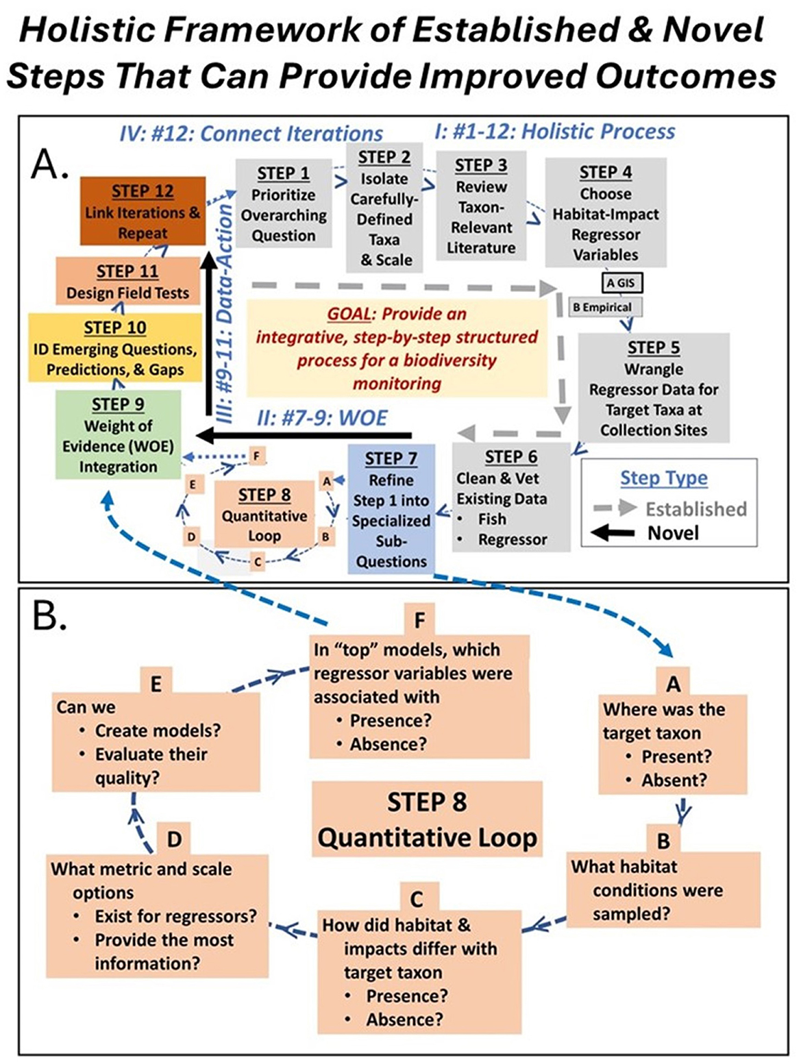
Figure 1. (A) Our 12-step iterative, adaptive management framework tool, in which (B) our 6 sub-step quantitative loop is embedded (Step 8). This figure summarizes our framework tool concept. Gray boxes are established steps that are currently used in many data collection-analysis designs (Steps 1–6). Colored boxes are partially (Step 8) or totally novel (Steps 7, 9–12) components of our framework. The multi-iteration expectation is that teams will go around the framework cycle many times for complex questions. Roman numerals (I–IV; blue text) indicate the advantages of following our framework compared to the use of select, isolated steps, and are reviewed in the discussion.

2.2 Steps 1–2

In step 1, management-researcher teams will strategically prioritize an overarching question of substantial scientific and conservation interest (Figure 1A). In step 2, the team selects a target taxon, spatial scale, and time period of interest. For both Steps 1–2, the rationale must be documented to maintain a historic record for future planning, ensure the continuity of the framework across staff and leadership changes, and to justify specific data-driven activities to outside interests. Realistically, a limited amount of information can be obtained in a single project (or a single framework tool iteration). If too many questions are asked at one time or too many taxa and scales identified, none will be answered satisfactorily. However, emerging questions, taxa, and scales can be addressed in additional, linked framework iterations.

2.3 Step 3–4

Two established and one novel types of literature reviews, used in step 3, provide context. First, per standard practice, manager-researcher teams will summarize which habitat and impact variables have been addressed in the current peer-reviewed literature for the prioritized taxon at relevant spatial-temporal scales. Second, as is typically done, teams will identify which of these habitat and impact regressors are available at the sites where the target taxon was sampled. Third, as a novel literature review procedure, we propose that benefits will accrue if teams also format quantitative literature results to match the axes and scale of their intended statistical model output (e.g., Table 1, columns 5–6, Y axis = probability of presence, X axis = regressor value). This quantitative standardization of results will allow an explicit comparison of expected (literature predictions) with observed (current study statistical output), will ensure shared goals across studies, and will identify gaps across studies that require future clarification. In Step 4, as is a common component of many data collection and analysis plans, teams select habitat (physical features) and impact (anthropogenic effects) variables relevant to the target taxon, while documenting the rationale, strengths, and weaknesses of these decisions.

Table 1

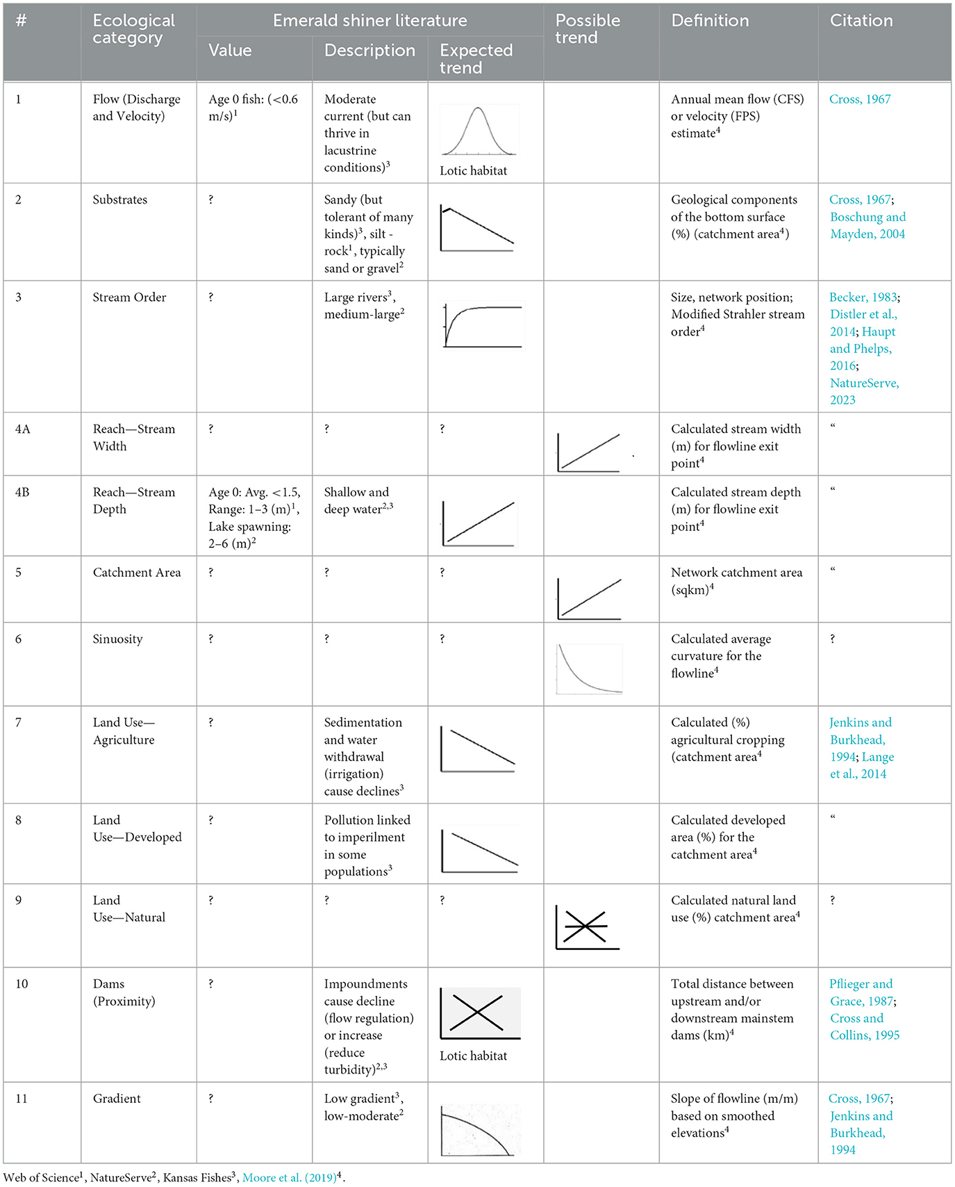
Table 1. Literature predictions for how ecological regressors might affect Emerald Shiner presence for the 11 ecological categories used here including numerical values; description of response; our interpretation of the expected trend (X axis = ecological category, Y axis = Emerald Shiner presence); a hypothesized possible trend; definition; and citation. ? = no KS information.

2.4 Steps 5–6

Steps 5–6 are essential but not novel parts of our framework tool. Ensuring that compiled data sets are accurate, understood, and appropriately interpreted is a priority in adaptive management frameworks that connect and build on existing datasets. In Step 5, using select GIS datasets, teams wrangle multiple habitat and impact metrics at the latitude and longitude at which taxon samples were collected. Ecological categories of habitat and impact factors, regressor definitions, and specific GIS databases that we used for our biodiversity conservation question are described in objective 2 (proof-of-concept results). In Step 6, researcher-manager teams apply quality control checks to the taxon and habitat-impact regressor databases. The data wrangling and data cleaning processes we used in steps are described elsewhere (e.g., Chapman, 2005; Terrizzano et al., 2015; Rattenbury et al., 2017; Ilyas and Chu, 2019).

2.5 Step 7

Step 7, the first novel component of our framework tool, refines the overarching question of interest (Step 1) into specialized, connected sub-questions that are each paired with an individual visualization or analysis (Sub-steps 8A–F). A common issue that emerges with the analysis of large datasets addressing complex questions is that individual quantitative activities can unintentionally diverge from the overarching question. Step 7 maintains a unified focus by preventing unplanned fracturing of directions across quantitative tools that can limit subsequent integration. Below, individual sub-questions are listed with their paired quantitative step (visualization, analysis, or model; Sub-steps 8A–F). Our specific sub-questions, listed below, explore drivers of presence-absence of native fish taxa, but like steps 1–6, they can be modified for other specific projects as needed.

2.6 Step 8

The quantitative loop in Sub-steps 8A–F (Figure 1B) illustrates our visualization-and-analytical workflow. For this step, we combined presence absence maps, proportional symbol maps, histograms, box plots, probability plots, ridgeline plots, pie plots, correlations, multiple logistic regressions, and 10-K fold cross validations [ggplot2 (Wickham, 2016); ggridges (Wilke, 2022); plotly (Sievert, 2020); corrplot (Wei and Simko, 2021); MuMIn (Bartoń, 2022); caret (Kuhn, 2022); and tidyverse (Wickham et al., 2019; R Core Team, 2022)]. These visualizations and analyses worked well for our taxa, system, and questions, but other analyses might be appropriate for other projects.

2.6.1 Sub-question (8A): where was the target taxon present or absent?

In this sub-step, data analysts can map and discuss taxon presence and absence related to statewide spatial patterns, region-specific patterns, gaps in distribution, and patterns of spatial heterogeneity (e.g., are there a few presences in a sea of absences or a few absences in a sea of presences).

2.6.2 Sub-question (8B): at what habitat conditions was the target taxon sampled?

To interpret visualizations and statistical tests, data analysts need to know what existing field conditions were sampled. Using a hypothetical example, if a given taxon was caught only in small streams and large streams were not sampled, little support would exist for the conclusion that this taxon was only found in smaller streams. For this statistical sub-step, we recommend two complementary visualizations. First, we constructed histograms [i.e., frequency distribution (Y axis) for specific values for each potential habitat or impact regressor (X axis) across all sample sites] to illustrate how often each quantitative condition was sampled. A second visualization, statewide proportional symbol maps in which symbols for target regressors vary in size, helped to visualize the geographic location and magnitude of habitat and impact regressors at the taxon sample sites.

2.6.3 Sub-question (8C): how did habitat and impact variables differ where the target taxon was present or absent?

We recommend two types of exploratory visualizations (boxplots and ridgeline plots) to better understand differences in habitat and impact conditions at sites where an individual taxon was present compared to sites where the same taxon was absent. As a first visualization, box plots can be used to compare discrete distributional benchmarks (e.g., central tendency, quartiles) between presence-absence sites for each habitat and impact variable. As a second visualization, ridgeline plots (i.e., a stacked set of distributional density plots that create the impression of a mountain range) visualized the full extent of continuous distribution overlap for each variable at sites where a taxon was present or absent. Both plots can be used to help interpret species distribution model results (Sub-steps 8E–F).

2.6.4 Sub-question (8D): what metric and scale options might best identify differences between sites where the target taxa was present or absent?

Sub-step 8D can compare and prioritize the performance of multiple GIS-related metrics and scales for a given ecological category of regressors. For example, in the ecological substrate category (i.e., soil components of the land surface), publicly available GIS data may include clay, silt, sand, and rock fragment metrics at point, flowline, catchment, network flowline, and network catchment scales (listed in order of increasing size). However, in a parsimonious statistical model, data analysts typically select a single metric-scale for each ecological category. To systematically choose and justify best metric-scales for each ecological category, we recommend two tools (i.e., exploratory boxplots and best-subset logistic regressions). As a first visualization tool, we used exploratory boxplots to identify the metric-scale option that was most likely to detect a difference (i.e., had the least overlap between sites where the target taxon was present or absent). For example, if exploratory boxplots showed that geological substrates such as % silt differed little between presence and absence sites and % sand differed greatly across site categories, we chose % sand as the initial, default geological metric for the substrate ecological category in the multiple logistic regression (Sub-steps 8E–F). As a second analysis, we used best-subsets multiple logistic regression (e.g., Hosmer et al., 1989; King, 2003; Zhang, 2016) to compare and prioritize multiple metrics within ecological and scale categories [(1) metrics within an ecological category, and (2) the same metric at different scales].

2.6.5 Sub-question (8E): can we create models and evaluate their quality?

For Sub-step 8E, we undertook the following actions to create multiple logistic regression models (referred to throughout as all-ecological-categories models) that identified which habitat and impact variables influenced the probability of target-taxon presence or absence. (1) We selected one scale-specific metric from each ecological category based on the results of Sub-steps 8C–D. (2) We balanced our dataset by randomly removing data points from the larger of the two classes (usually absences) until presences equaled absences (Salas-Eljatib et al., 2018). (3) We examined correlations among model-specific regressors (Appendix Figure 1), and one of any highly correlated (P > 0.7) pair was removed (Mukaka, 2012). (4) We fit multiple logistic regression models to uncorrelated metrics.

2.6.6 Sub-question (8F): in the top models, which habitat-impact regressors were associated with taxon presence or absence?

In Sub-step 8F, we summarized which habitat and impact regressor variables were most important in the logistic regression. (1) For top models, defined as models with delta Akaike Information Criterion (ΔAIC) ≤ 2 (Anderson and Burnham, 2002), we evaluated the size and direction of the parameter estimates, error size, and parameter-specific P-values. (2) For regressors with P ≤ 0.05 in the top models, we constructed probability plots (Y axis = probability of presence, X axis = magnitude of individual regressor values) to visually examine the relationship between significant regressors and target-taxon presence and absence. We appreciate that P-values do not have an exact meaning for messy field data, and here we only used them to prioritize trends (Murtaugh, 2014). (3) To evaluate the accuracy of the model, we applied a 10-K fold cross validation to identify the percent of the model classifications that were correct (Manorathna, 2020). (4) We tested multicollinearity assumptions using variable inflation factors (VIF; car, Fox and Weisberg, 2018) and condition numbers (CN; klaR, Weihs et al., 2005). A VIF < 10 has been considered an acceptable rule of thumb for detecting multicollinearity although some analysts suggest investigating lower values (VIF < 5–10; Menard, 2002; Vittinghoff et al., 2005; James et al., 2014). A CN < 30 has been considered an upper level for acceptable multicollinearity but again some analysts suggest investigating lower values (CN < 10–30; Freund and Littell, 2000; Salmeron et al., 2022; Roever et al., 2023). (5) Finally, we calculated the D² statistic for the top model to observe the amount of variance that the model explained (stats; R Core Team, 2022). Instead of calculating accumulated error rates across sub-steps, we report the quantitative steps undertaken in detail. Our use of logistic regression follows an established statistical process for a frequently used species distribution model. However, specifics of Sub-step 8E–F are adaptable across projects because our framework allows for the systematic testing, comparison, and addition of other modeling and visualization tools (e.g., random forests, boosting, bagging, stacking, and alternate modeling techniques). The novelty we add lies in the explicit integration of quantitative literature predictions, exploratory visualizations, and a regression model to identify data connections-gaps and suggest future actions (Steps 3, 9–12).

2.7 Step 9

Weight of evidence integration (WOE; Step 9) is the novel step that summarizes what was learned cumulatively across quantitative tests of six specific sub-questions (Figure 1B). Here, we implement WOE integration by comparing descriptive visualizations of habitat composition at presence and absence sites. Other ways to operationalize WOE integration include comparing model coefficients to trends expected from literature, or comparing overall habitat variable distributions across the area of interest in relation to the model coefficients. Our WOE integration of all results from multiple visualizations and analyses prevents subjective omission of inconvenient results which can introduce ambiguity when different analysts selectively interpret the results from their chosen approach. In summary, WOE uniquely pinpoints: (1) consistent insights on which to build; (2) ambiguous insights that demand focused attention in future sampling-analysis; (3) gaps in understanding and data availability, and (4) future directions that prioritize and guide thoughtful new data collection and analyses. We provide five specific examples of the benefits of WOE integration below in our proof-of-concept example in the results section (objective 2).

2.8 Steps 10–12

The next four novel steps convert WOE data syntheses into future actions. Specifically, teams will translate the WOE integration into relevant new questions, data-ready predictions, and testable hypotheses (Step 10). Realistic data collection regimes (general and specific) can then be identified to address these questions-predictions-hypotheses, and inform gaps (Step 11). Our expectation is that planners, administrators, and biologists agree to follow up on each framework iteration by subsequently collecting and analyzing the recommended data to address the emergent questions-predictions-hypotheses, and link datasets to accumulate understanding (Step 12). We provide multiple examples of these data-action steps below in our proof-of-concept (objective 2) in the results section.

3 Proof-of-concept results for our framework tool

3.1 Organization of the results section

For objective 2, we show how new ecological and management insights and options for actionable science emerge from our framework tool. When the results for the 12-step framework tool are viewed together, the specific analysis foundation (Steps 1–6) sets up the individual quantitative results (Steps 7–8), upon which the innovative WOE integration, application, and connections emerge (Steps 9–12). For best results, all steps, sub-steps, sites, and regressors are systematically analyzed and recorded as part of the information accumulation process. However, reporting these voluminous results here is impractical. For readability, we only show two types of visualization results. (1) We review results for substrate (geologic bottom materials) to illustrate how a single regressor behaved across all visualization sub-steps (Sub-steps 8B–D). (2) We review results for a pair of regressors [order, land types; Sub-steps 8C–D)] that were significant in our all-ecological-category regression models (Sub-steps 8E–F) to add ecological understanding. For space, we also limit data synthesis-to-action examples (Steps 9–11) to five regressor variables (order, substrate, sinuosity, dams, natural land use).

3.2 Steps 1–2, 4–6

In our proof-of-concept results, Steps 1–2, 4–6 identify directions that provide the foundation for the first framework iteration (overarching question, taxa, data steps). We chose Emerald Shiner (Notropis atherinoides) for all time periods of data collection across the statewide Kansas scale [Kansas Geological Survey (KGS), 2012] to address the general question of “if and why might a specific, native stream fish taxon be present or absent at specific locations?” Emerald Shiner has a wide U.S. distribution (Page and Burr, 2011), is an ecologically important fish in many aquatic food webs (Etnier and Starnes, 1993), has some physical habitat associations, but occurs in diverse habitats (Distler et al., 2014), and had a high number of presences in our existing dataset. We used monitoring data from 8,844 fish samples collected at 7,872 unique statewide stream locations of which 70% were collected between 2010 and 2021 (Figure 2A). We identified 11 fish taxa-relevant ecological categories: (1) flow, (2) substrate, (3) order, (4) reach size [(A) width, (B) depth], (5) catchment size, (6) sinuosity, (7) agricultural land, (8) developed land, (9) natural land, (10) dam characteristics (e.g., dam proximity measured as total mainstem distance to adjacent upstream and downstream dams), and (11) gradient. Definitions of variables are shown in the second to the last column of Table 1. For land and impact regressors, we used 2021 data to match the timing of most fish collections. At the latitude and longitude at which fish taxon samples were collected, we compiled multiple metrics for these 11 ecological categories at multiple scales using select GIS datasets (Table 2). As an illustration of a benefit of using GIS for habitat and impact variables, we were able to obtain regressor data for most of the 7,872 locations in our fish monitoring database, compared to 1,679 sites at which matching empirical habitat data were available (Reed, 2023). In future iterations, other abiotic-biotic variables, databases, and years can be examined.

Figure 2

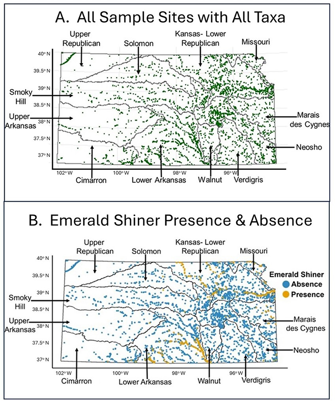
Figure 2. (A) Map of our study area with all fish sampling locations indicated. Each green dot represents a unique sample site. (B) Fish sample sites at which Emerald Shiner was present (gold dots; n = 1,131 total presences at 903 unique locations) or absent (blue dots; n = 7,713 total absences at 7,076 unique locations). On both panels, names of major river basins in Kansas are indicated. This visualization corresponded to Sub-step 8A in our quantitative loop.

Table 2

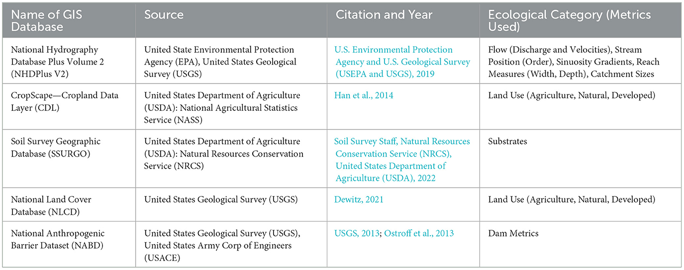
Table 2. GIS database name, source, citation, year, ecological category, and metrics used to wrangle habitat and impact data for our “12+6 step adaptive management framework” tool.

3.3 Step 3

Our two established literature reviews, described in the methods section, identified choice of ecological categories of regressors. From our novel quantitative literature review, we predicted that Emerald Shiner presence will be more likely at sites with intermediate flows (ecological category 1; Table 1) and increased stream size (ecological categories 3, 4, 5) because in Kansas streams this “large river” fish is often caught at sites with moderate currents. We predicted that the probability of Emerald Shiner presence is less likely at sites with extreme bottom substrate sizes (ecological category 2), more land alterations (ecological categories 7, 8), and with high gradients (ecological category 11) because Emerald Shiner is often associated with sand beds, limited agriculture, restricted human land development, and low to moderate gradients. Little is known about the effect of sinuosity on this taxon (ecological category 6). Similarly, little data exist on Emerald Shiner response to natural land (ecological category 9), but this common native fish is widely distributed so multiple outcomes are possible. We also predicted multiple outcomes for dam proximity (ecological category 10) because dams both reduce flow (negative effect) but also reduce turbidity (positive effect).

3.3.1 Where was the target fish taxon present or absent (8A)?

Emerald Shiner was widely distributed across the state of Kansas (presence = 1,131 samples at 903 unique locations, absence = 7,713 samples at 7,076 unique locations; Figure 2B). Regionally, this taxon was present in south-central Kansas (Lower Arkansas Basin, n = 696) and northeast Kansas (Kansas-Lower Republican Basin, n = 354). Emerald Shiner was largely absent from watersheds in the western third of the state. Both the frequency of occurrence and regional distribution of Emerald Shiner provided important information about this species.

3.3.2 At what habitat conditions was the target fish taxon sampled (8B)?

Histograms showed which habitat conditions were most common where fish were sampled and proportional symbol maps added a spatial component. Specifically, histograms illustrated that silt is a very common substrate in Kansas (Figure 3A). Proportional symbol maps added information on where geographically-high percentages of silt substrate were found (eastern and north-central KS; Figure 3B; large, bright royal-blue circles). Although many fish sample sites had low proportions of sand substrate (Figure 4A), sand was most common in the south-central region and select areas of northeast Kansas (Figure 4B).

Figure 3

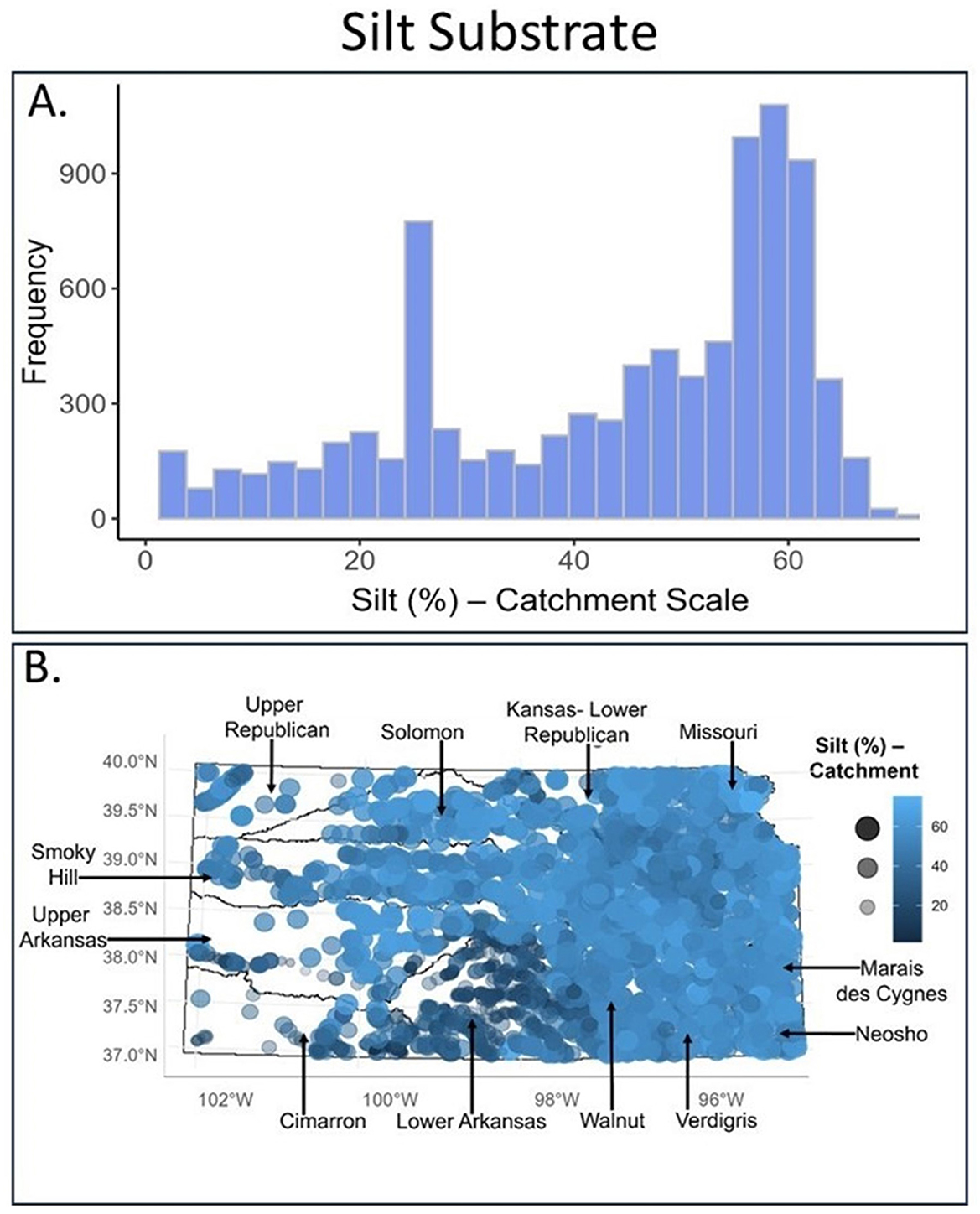
Figure 3. For silt substrate, shown are (A) a frequency distribution plot and (B) a proportional symbol map for all samples taken within our study area (calculated at the local catchment area scale). For proportional symbol maps, dot size (small–large) and color (dark blue to light blue) both indicate the relative proportion of silt substrate at that site (e.g., a large, royal blue dot indicates high amounts of silt whereas a small, dark blue dot indicates low amounts of silt substrate). Major river basins are indicated. These visualizations corresponded to Sub-step 8B in our quantitative loop.

Figure 4

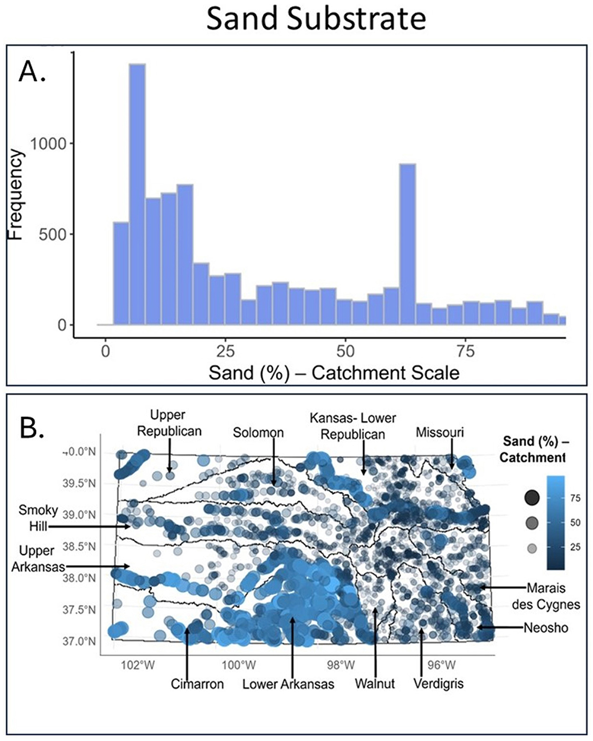
Figure 4. For sand substrate, shown are (A) a frequency distribution and (B) proportional symbol map for all fish samples taken within our study area (calculated at the local catchment area scale). For proportional symbol maps, dot size (small–large) and color (dark blue to light blue) both indicate the relative proportion of sand substrate at that site (e.g., a large, royal blue dot indicates high amounts of sand substrate whereas a small, dark blue dot indicates low amounts of sand). Major river basins are indicated. These visualizations corresponded to Sub-step 8B in our quantitative loop.

3.3.3 How did habitat and impact variables differ where the target taxon was present or absent (8C)?

Ridgeline plots showed how the distribution varied between presence and absence sites for each regressor. For substrate, Emerald Shiner tolerated some level of adverse silt substrate in the northeast region (Figure 5A), but was positively associated with sand substrate where available (Figure 5B). For stream order, ridgeline plots showed that Emerald Shiner was present in stream size orders 7–8 and generally absent from smaller stream sizes (stream orders ≤ 6; Figure 5C).

Figure 5

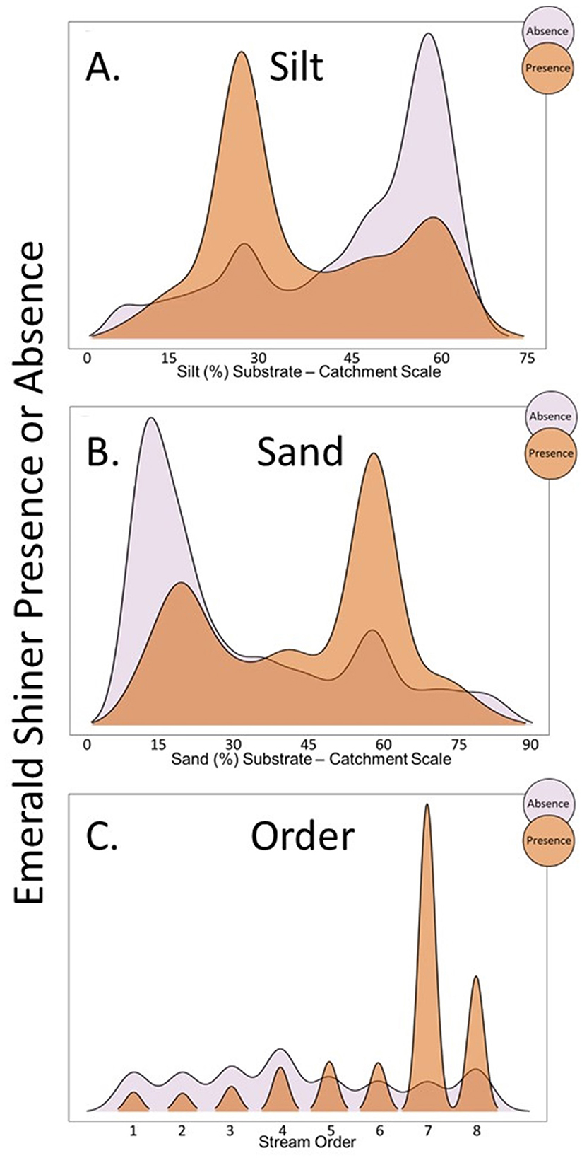
Figure 5. Ridgeline plots showing how proportion of samples in which Emerald Shiner were present was related to (A) silt substrate (%), (B) sand substrate (%), and (C) stream order. Orange ridges are sites where Emerald Shiner was present, and purple ridges are sites where Emerald Shiner was absent. These visualizations corresponded to Sub-step 8C in our quantitative loop.

3.3.4 What useful metric and scale options exist (8D)?

In our proof-of-concept, we used this sub-step to select a single metric-scale for each ecological category used in our regression analyses (Figures 6A–O). We prioritized two substrate scales (e.g., flowline, catchment) for use in our all-ecological-categories regression models (Sub-steps 8E–F). Specifically, when we used paired (presence vs. absence) box plots to compare substrates at three scales (point, flowline, catchment; sand (Figures 6G, H), and silt (Figures 6J, K) measured at the flowline and catchment scales, showed the greatest differences between conditions where Emerald Shiner was present or absent.

Figure 6

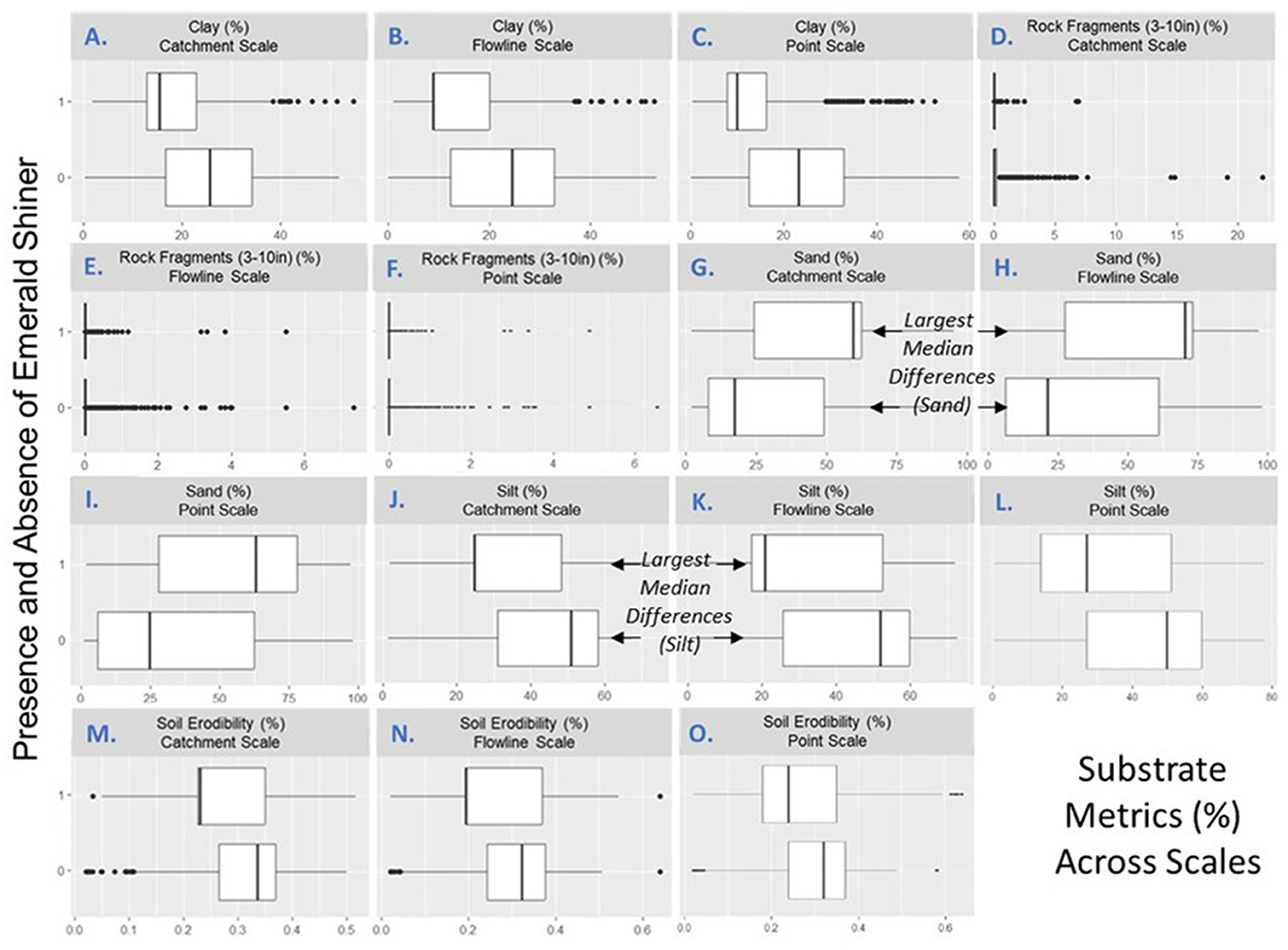
Figure 6. Boxplots of the distributions of substrate (A–L) and substrate-related metrics (M–O) at sites where Emerald Shiner was present or absent. Shown are median (thick black bar), quartiles (white box), and minimum and maximum (individual points). (A–C) clay at the (A) catchment, (B) flowline, and (C) point scale. (D–F) rock fragments (3–10 in) at the (D) catchment, (E) flowline, and (F) point scales. (G–I) sand substrates at the (G) catchment, (H) flowline, and (I) point scales. (J–L) silt at the (J) catchment, (K) flowline, and (L) point scales. (M–O) soil erodibilities at the (M) catchment, (N) flowline, and (O) point scales. Minimal overlap between presence and absence bars indicates that a specific metric-scale differs for sites where Emerald Shiner was present or absent. Box plots depict the minimum, first quartile, median, third quartile, and maximum, with outliers depicted as single points. This visualization corresponded to Sub-step 8D in our quantitative loop and helped select metrics for the all-ecological-categories multiple logistic regression.

We prioritized two natural land metric-scales (grassland, natural land metrics at the catchment and flowline scales) for use in our regression models (Sub-step 8E–F). Specifically, when five scales (point, flowline, catchment, network flowline, network catchment) for two natural land metrics (grassland, natural cover; Appendix Figures 2A–J) were plotted for Emerald Shiner presence and absence sites, (1) grassland at the catchment scale (Appendix Figure 2G) and (2) natural cover at the flowline scale (Appendix Figure 2I) exhibited the greatest median difference between sites at which Emerald Shiner was present or absent. Across-scale comparisons can be added as separate variables in future framework iterations.

3.3.5 Can we create models and evaluate their quality (8E)? In top models, which variables were associated with target fish taxon presence and absence (8F)?

Two “top” models with a ΔAIC ≤ 2 had five significant regressors representing the same ecological categories (P ≤ 0.05; Table 3A, B): (1) silt substrate, (2) stream order, (3) sinuosity, (4) agricultural land (pasture or cultivated crops), and (5) natural grassland. In our analysis, 96% of regressor variables exhibited VIF values < 5, and 100% exhibited VIF values < 6. Further, 82% of our regressor variables had CN values < 10, and 100% exhibited CN values < 20. Of the six models that used a single uncorrelated metric from each ecological category, the top model with the highest accuracy (Table 3A) predicted presence and absences correctly 74% of the time (Appendix Tables 1A, B) and explained 23% of the variation between the balanced sample classes for Emerald Shiner (D²; Appendix Table 1C). All flow variables, one reach measure [width], and one classification of natural land were removed because they were highly correlated with other regressors. Correlated substrates and land types were tested in separate models. Balancing presence and absence sample sizes did not change mean values substantially (Appendix Table 2).

Table 3

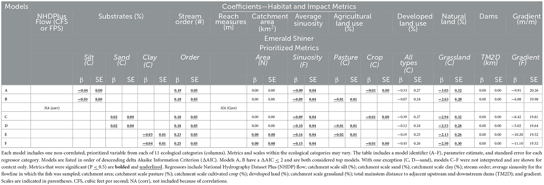
Table 3. Six multiple logistic regression models (rows A–F) for Emerald Shiner (Y response = probability of presence).

In both top models, influential regressors had the same directional effects on probability of Emerald Shiner presence (Table 3A, B) An increase in the small substrate, silt, decreased the probability that Emerald Shiner would be present at a site (Table 3A, B; Figure 7A), and an increase in sand (in a different model) increased the probability of Emerald Shiner presence (Table 3C, D; Figure 7B). As stream order increased so did the probability of Emerald Shiner being present (Table 3A, B; Figure 7C). The probability of Emerald Shiner presence was inversely related to sinuosity (Table 3A, B; Figure 7D). Both types of agricultural land (pasture cover and cultivated crops) were inversely related to the probability of Emerald Shiner presence (Table 3A, B; Figures 7E, F). Percent of grassland decreased the probability of Emerald Shiner being present at a site (Table 3A, B; Figure 7G). Clay substrate, catchment size, total mainstem distance between dams (TM2D), and gradient were never significant in top models; sand and silt substrates were never in the same model (Table 3).

Figure 7

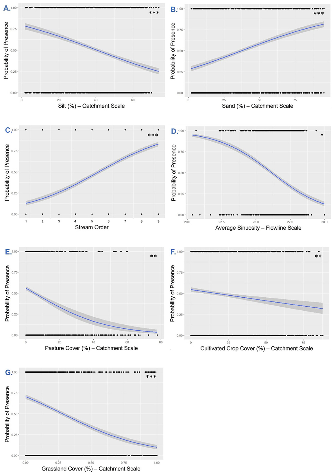
Figure 7. Probability plots for all metrics (P ≤ 0.05) included within the top model(s) for presence of Emerald Shiner. (A) Silt substrate (%)—Catchment Scale, (B) Sand substrate (%)—Catchment Scale, (C) Stream Order, (D) Sinuosity—Flowline Scale, (E) Agricultural land—Pasture (%)—Catchment Scale, (F) Agricultural land—Crop (%)—Catchment Scale, (G) Natural land—Grassland (%)—Catchment Scale. The level of significance was used to prioritize regressors for interpretation and can be viewed in the top left corner (Significance Codes: “***”P < 0.001; “**”, 0.001 < P < 0.01; “*” 0.01 < P < 0.05). This analysis corresponded to Sub-step 8-F in our quantitative loop.

3.4 Steps 9–12

Weight of evidence integration (WOE; Step 9) coordinated individual results, and connected present data and future actions. As such, this step provided the centerpiece and payoff for our framework tool. Specifically, WOE integration detected areas of agreement for which no additional data collection-analysis is required, and identified ambiguous results that require additional data clarification. For example, below we show how combining literature predictions (Step 3), and multiple maps and visualizations (Sub-steps 8A–D) aided ecologically-convincing and quantitatively-consistent interpretations of the all-ecological-categories multiple logistic regression models (Sub-steps 8E–F). WOE integration also uncovered emerging questions, predictions, and gaps (Step 10) that would be beneficial to address in future data collection and research (Step 11). Testing of field predictions (in iteration 2) that were identified in steps 1–10 of iteration 1 linked datasets and across-iteration analyses (Step 12).

For some variables (e.g., agriculture, gradient, order), the combined interpretation of all visualizations (Sub-steps 8A–D) and the all-ecological-categories logistic regression analysis (Sub-steps 8E–F) were similar across quantitative steps and consistently trended as expected from literature predictions (Step 3). As an example, the adverse effect of agricultural land (Steps 8C, E–F; Figures 7E, F) was expected from literature predictions (Step 3; Table 1, line 7) even though pasture (grass monocultures often associated with livestock grazing; Broom, 2019) and cultivated crops (any land used for annual crop production such as wheat, corn, sorghum, and soybean; Danielson et al., 2016; Laird, 2022) are very different. In the low-elevation, rural state of Kansas, the lack of significance for developed land and gradient (Sub-step 8C, E–F) was not unexpected given available conditions (Sub-step 8B), and, as such, was consistent with literature expectations (Step 3).

We also expected the consistent, observed positive relationship between stream order and Emerald Shiner presence from the literature. WOE integration (Step 9) informed the role of stream order on Emerald Shiner distribution by combining insights on representativeness of sampling conditions (Sub-step 8B; histograms, proportional symbol maps), values at which Emerald Shiner was present or absent (Sub-step 8C; ridgeline plots), variable behavior across scales (Sub-step 8D; paired boxplots), and the multiple logistic regression (Sub-steps 8E–F). The combined WOE for Emerald Shiner use of larger streams reinforced the importance of width, depth, order, and catchment area for Emerald Shiner in the literature (Distler et al., 2014; Haupt and Phelps, 2016). The WOE integration also identified useful and testable questions about interactions among system size and geomorphology of instream habitats (Step 10) such as “Can a detailed quantification of multiple aspects of channel morphometry (width vs. depth within an order) better predict taxon presence?” A sampling plan that addresses this question (Step 11) could select a range of sites where Emerald Shiner is present and absent, then quantify stream morphometry (width, depth, order) to assess if this taxon is more common at different combinations of these size parameters (e.g., wide-deep vs. wide-shallow vs. narrow-deep). Following this analysis, the results of predictions and additional sampling could be incorporated into future iterations (Step 12).

Ambiguous and inconsistent trends emerged for other regressors (substrate, dams, natural land) that did not agree with predictions from the literature. For example, substrate did not trend as expected. We expected this taxon to be solely associated with sand substrate (Table 1, line 2), but silt emerged as the most influential substrate variable. This ambiguous trend was better understood in the context of the combined WOE integration [fish maps (Sub-step 8A), histograms and proportional symbol maps (Sub-step 8B), and ridgeline plots (Sub-step 8C)]. Specifically, Emerald Shiner was associated with sand substrate when it was available (Figures 4A, B, 5B). Silt substrate, which can impair foraging success and population persistence of even tolerant sight-feeders like Emerald Shiner (Pflieger and Grace, 1987; Jenkins and Burkhead, 1994), was common statewide and also regionally distributed (Figures 3A, B). Combining these visualizations with the multiple logistic regression, a geographic substrate association emerged. Emerald Shiner was present where the beneficial sand substrate was common and the potentially harmful silt substrate was reduced (south-central region). Emerald Shiner was not often present in regions where silt substrate dominated without sand substrate (southeast region). However, the somewhat tolerant Emerald Shiner occurred in some areas where both sand and silt substrates co-occurred (northeast region).

As a result of the WOE integration (Step 9), three testable new questions (Step 10) about the interconnected roles of co-occurring sand (potentially beneficial) and silt (potentially harmful) substrates were identified. (1) “What is the minimum proportion of a “positive” substrate that is needed for this fish to thrive (e.g., sand)? (2) What is the threshold at which adverse substrates (e.g. silt) can no longer be tolerated? (3) Are some common taxa (e.g., Emerald Shiner) better able to tolerate silt compared to uncommon native species in need of conservation (e.g., Plains Minnow)?” Collecting detailed empirical substrate data (especially co-occurring silt and sand) at a set of sites where Emerald Shiner (and other less common native taxa) are present or absent (especially in the northeast and south-central regions of Kansas) would link these WOE-derived questions to future directions for data collection (Step 11). Focusing on interactions among multiple substrates would provide more utility for future planning (Step 12) than simply correlating fish taxon distribution to a single, commonly-used substrate.

Sinuosity (significant effect) was a regressor for which we had no clear expectations because of lack of published information (Step 3, Table 1, line 6), but for which our framework provided guidance for future actions. WOE integration (Step 9) of multiple quantitative steps (Sub-steps 8C, E–F) consistently identified that Emerald Shiner presence was inversely related to sinuosity (e.g., Figure 7D). Instream complexity (e.g., channel units, bends, sandbars) is ecologically important for fish (Kaufmann et al., 2022; Hart, 2023) and may be related to sinuosity. Because Emerald Shiner typically shoal in straight, simply-structured stream channels or runs (Jenkins and Burkhead, 1994), our framework raises an intriguing question on which to focus future data collection (Step 10). Specifically, “Can sinuosity (an easily measured GIS variable) predict ecologically-relevant (but difficult-to-measure) instream habitat complexity?” The relationship between instream complexity, and sinuosity could be tested by measuring channel units, bends, sandbars (instream complexity) and sinuosity at a subset of sites at which Emerald Shiner is either present or absent (Step 11). Whether this taxon is more often present at non-sinuous locations (simpler habitat) can be integrated into future iterations (Step 12).

The metric that we used for dam presence (non-significant effect) was another regressor for which we had no consistent expectations because of lack of published information about fish relationships to specific dam metrics (Step 3; Table 1, line 10). Again, WOE integration provided guidance for future actions. Dams are complex disturbances that often harm stream fish (e.g., Barbarossa et al., 2020), but environmental professionals know relatively little about which dam metrics best quantify the adverse effect of dams on non-migratory, prairie stream fish. Using a recent database of GIS dam metrics (Ostroff et al., 2013), we did not find specific impacts of the dam proximity metric on Emerald Shiner (Step 8; Table 3). However, through our WOE iterations (Step 9), we identified a gap [i.e., when, where, and how do different dam metrics influence native fish taxa]. Future iterations of question-directed analyses can fill this gap (Step 10). Promising questions include (1) “What are the differential effects of related metrics (dam proximity, number, density, inter-dam distance)? (2) Does the direction of dam location matter relative to the fish sample site (upstream or downstream)? (3) Which scales of dam effects are consistently more influential (local or watershed)? (4) How do different fish taxa respond to these dam metrics? (5) Are there accumulated and interactive dam effects? Future analyses can be undertaken with existing data at a selection of sites with and without the target taxon to assess which dam metrics differ between presence and absence sites (Step 11). Thus, for the ecological and impact category, dams, our framework provided a systematic process for using existing data to fill gaps.

Emerald Shiner response to natural land (Step 3, Table 1, line 9; Figure 7G) was a puzzler (Steps 8–9). In general, the literature regarding land and prairie stream fish is very limited (Step 3). Despite ambiguity of these results, our framework identified useful questions about natural land for future analyses (Step 10) such as “Does natural land have real adverse effects on prairie fish (and why) or is this metric simply an amalgamation of different land types that has no clear ecological meaning?” Analyzing relationships among different subtypes of natural land and between these subtypes and sites at which Emerald Shiner is present or absent (Step 11) would help answer these questions and facilitate future directions to accumulate a better understanding of the role of this regressor (Step 12).

4 Discussion of the benefits of our framework tool

4.1 Overview

Using our framework tool with existing monitoring data identified testable questions-predictions-hypotheses for future data-action connections. Below, we review four take-home messages that show benefits of our adaptive management framework tool.

4.2 Take home message 1. Value of the systematic use of our holistic structured process

Using all framework tool steps together can provide improved outcomes (Figure 1A—I). A realistic expectation is that for every major conservation question of interest, a team of professionals will go around our 12+6 step framework multiple times to accumulate required understanding and relevant guidance. Although intellectually obvious, making these links across steps and iterations is conceptually and operationally challenging. In our holistic framework tool, established steps (Steps 1–6) provided the foundation. WOE data interpretation (Step 9) of sub-question-focused visualizations (Step 7, Sub-steps 8A–D), and a species distribution model with probability plots (Sub-steps 8E–F) identified important unanswered questions, testable predictions, and gaps (Step 10). These information needs can be examined in the future with a realistic and focused data collection plan (Step 11). The result is a practical plan to connect data and insights across projects, framework steps, and framework iterations (Step 12). As examples of useful outcomes, we identified consistent areas of consensus on which to build (order, agriculture, gradient), areas of ambiguity which require clarification (substrate), clearly addressable gaps (sinuosity, dams), and a more puzzling disparity (natural land). Another important gap that we identified was that specific quantitative literature predictions often did not exist for most regressors at the scale and precision that matched analysis outputs. Providing data-driven predictions for literature expectations at relevant state, region, and global scales should be a priority in the future as this lack of realistic expectations affects interpretation, confidence in the analysis, and ability to prioritize future workplans.

4.3 Take home message 2. Utility of weight of evidence (WOE) integration and associated predictions

WOE integration is a unique aspect of our framework tool that packages quantitative conservation data differently, and provides more productive outcomes than a single isolated analysis presented alone (Figure 1A—II). Within the context of our framework, WOE for order, substrate, sinuosity, natural land, and dams provided five useful future directions reviewed in the results section [e.g., (1) potential utility of geomorphology-stream size categories (order, width, depth, catchment area), (2) need for multiple upper and lower substrate thresholds, (3) possible applications of sinuosity to instream habitat complexity, (4) potentially confounding effect of isolated vs. aggregated natural land categories, and (5) the need to tease apart the role of specific dam metrics]. In many traditional data analyses, when analysts adhere to specific statistical significance thresholds from a single favored quantitative approach, conflicting approach-specific interpretations can lead to unproductive disagreements amongst professionals using different statistics. In contrast, the philosophy underlying the WOE concept is that for complex issues (e.g., decision-making, risk assessment), integration of multiple pieces of evidence that may agree or disagree is required (e.g., Hong et al., 2018; Mehta and Rietjens, 2023). Thus, WOE integration can lead to a discussion of future needs. As an example, if we had only interpreted the top model or a single visualization, we would not have identified the interacting roles of sand and silt substrates.

4.4 Take home message 3. Our framework facilitates implementation and guides future actions

Our framework tool is an example of an adaptive management plan for biodiversity monitoring that can be used immediately and can ultimately guide future actions (Figure 1A—III). Outside of harvest models and select other examples, relatively few adaptive management efforts provide detailed steps for specific resource management problems (Fontaine, 2011; Rist et al., 2013). The accuracy of our first-iteration, all-ecological-categories multiple logistic regression model for Emerald Shiner (Sub-steps 8E–F) was high (74% correct predictions) and produced consistently interpretable information about regressors that were (order, substrate, sinuosity, land) and were not (dams) influential. If we had followed a more narrowly-defined methodology, we might have published this single analysis as a final product. However, our iterative 12+6 step framework tool illustrated that a single result is not especially useful for complex conservation questions. Instead, an implementable step-by step iterative process, like our 12+6 step framework tool, that systematically accumulates knowledge to make better and better use of existing data is more likely to assist practitioners. Of course, definitive management actions related to restoration, stocking, human land and water modifications should be the ultimate goal of the applied analysis of monitoring data. However, because of the complexity of many natural resource problems, defensible science-based management regulatory actions do not always emerge from just a few data-driven studies. Often intermediate knowledge steps are required before specific science-based management actions can be recommended. Here, identifying regressors and sites to focus future data collection and restoration initiatives represent these intermediate actions that link data and decision-making.

4.5 Take home message 4. General advantages for coordination and planning

Our framework is adaptable to other questions, data, and systems (Figure 8). Panel A depicts the approach illustrated here in which a single iteration addresses a large multi-variable problem. Panel B illustrates an approach for which the question, system, literature, and data have been previously explored, and for which a more complex quantitative loop is the primary focus of the project. In the panel B example, Steps 1–6 may be addressed quickly because the specifics of the problem are well known. Using our framework on largely statistical projects can add practical benefits by linking all analyses together through WOE integration (Step 9), adding a data-action connection to each iteration (Steps 10–11), maintaining a unified focus on the original overarching question (Step 1), and directing linkages across iterations/projects (Step 12). Panel C illustrates a problem in which the specific questions are transformed into a series of focused hypotheses that are addressed sequentially (Step 7). In this third example, Steps 1–6 are addressed in detail in the first iteration, but may only be briefly considered in subsequent iterations. All variations of our framework explicitly embed past-present-future connections and management actions within each iteration. As a result our framework advances the spirit of the adaptive management concept.

Figure 8

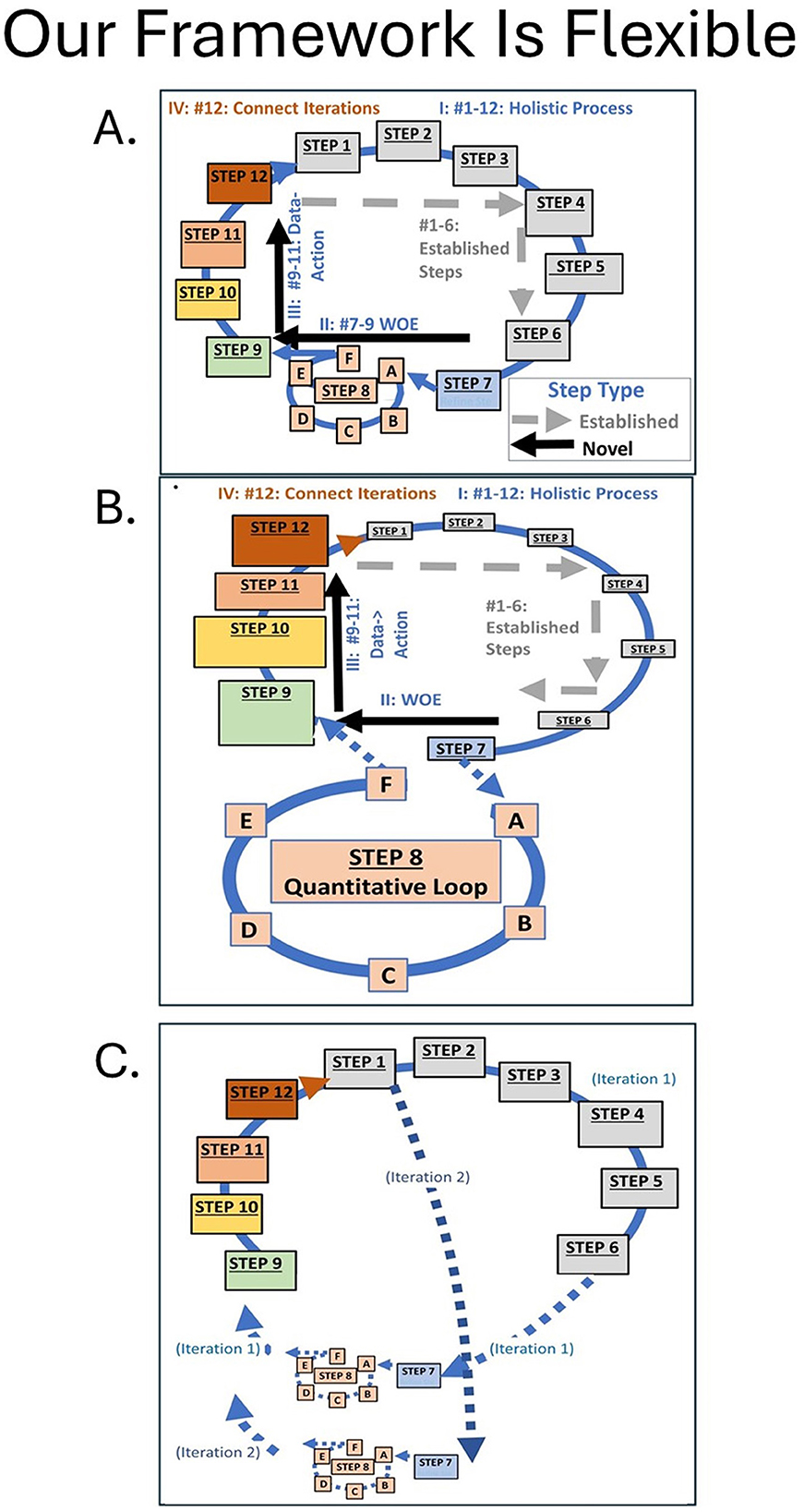
Figure 8. Three different configurations of our 12+6 step framework tool that have the same steps and provide the same advantages (Figure 1A, II, III, IV). (A) is the basic approach illustrated here in which a single iteration addresses a large multi-variable problem. (B) illustrates an approach for which the question, system, literature, and data have been previously explored and for which a more complex statistical analysis is the primary focus of the project. Note that (B) differs from a stand-alone species distribution modeling exercise because (1) the rationale for the model must be repeatedly reviewed and justified relative to previously identified goals (Steps 1–6) and (2) the framework requires that output explicitly be processed through WOE integration (Step 9), linked to testable predictions or data-ready questions (Step 10) with realistic and appropriate methods (Step 11), and coordinated with the next iteration (Step 12). (C) illustrates a problem in which the specific questions (Step 7) are transformed into a series of focused hypotheses that are addressed sequentially. Project C is thoughtfully-justified in an initial iteration (Steps 1–6) although steps 2–7 may or may not be major foci in future iterations. Then for each hypothesis and analysis (Steps 7, 8), the link to the overarching question is reassessed and adjusted as needed (dashed arrow) and results outputted into a WOE integration (Step 9) followed by a data-to-action sequence (Steps 10–11). In all options, Step 12 connects present and future data activities.

In summary, examining individual analyses and isolated datasets can limit the efficacy of conservation planning because multiple components, diverse stakeholders, and competing priorities intersect in non-academic, real-world conservation projects (Davis et al., 2006; Vidal and Marle, 2008). A good literature review is needed, but might not be easily attainable for some taxon or geographical areas. Our framework tool connected datasets and activities (Figure 1A—IV). For example, real time data analysis conducted in a professional group setting can lead to productive conversations about priorities (Mather et al., 2023). The framework needs to be tested on biota about which less is known, a process that is now possible with the step-by-step guide presented here. A future plug-and-play version of our framework with a dashboard of appropriate data layers could provide opportunities for teams of researchers and managers to regularly discuss data interpretation and future directions.

Data availability statement

Publicly available environmental datasets were analyzed in this study. The names of the repository/repositories and accession number(s) can be found in the article/Supplementary material.

Ethics statement

The animal study was approved by Kansas State University Institutional Animal Care and Use Committee. The study was conducted in accordance with the local legislation and institutional requirements.

Author contributions

OR: Conceptualization, Data curation, Formal analysis, Investigation, Methodology, Project administration, Visualization, Writing – original draft, Writing – review & editing. MM: Conceptualization, Data curation, Formal analysis, Funding acquisition, Investigation, Methodology, Project administration, Supervision, Visualization, Writing – original draft, Writing – review & editing. DO: Conceptualization, Data curation, Formal analysis, Investigation, Methodology, Visualization, Writing – review & editing. KN: Data curation, Formal analysis, Methodology, Writing – review & editing. VR: Visualization, Writing – review & editing. TM: Conceptualization, Data curation, Formal analysis, Methodology, Writing – review & editing. SP: Formal analysis, Visualization, Writing – review & editing.

Funding

The author(s) declare financial support was received for the research, authorship, and/or publication of this article. This project was funded through the Kansas Department of Wildlife and Parks (KDWP).

Acknowledgments

The project was administered by the Kansas Cooperative Fish and Wildlife Research Unit as a joint effort between Kansas State University, the U.S. Geological Survey, U.S. Fish and Wildlife Service, the Kansas Department of Wildlife and Parks (KDWP), and the Wildlife Management Institute. We thank KDWP for sharing the monitoring dataset. We thank Michael Madin, and Jean Francois from the Kansas State Department of Geography and Geospatial Analysis who have offered their expertise in R programming and spatial data analysis. Thanks also to colleagues who provided advice and access to datasets. Drs. Jane Rogosch, Trevor Hefley, Steve Chipps, Kayla Boles, and two reviewers provided useful comments and other assistance. We especially appreciate the assistance of the Kansas Department of Wildlife and Parks Ecological Services Section. Jordan Hofmeier provided valuable insights into conservation concerns highlighted within the Kansas State Wildlife Action Plan as well as substantial expertise in aquatic ecology. Regressor data are available from the authors upon reasonable request. Finally, we offer many thanks to Ryan Waters, a KDWP stream biologist who is an expert source of knowledge about prairie stream fish. Any use of trade, product, or firm names is for descriptive purposes only and does not imply endorsement by the U.S. Government. A review of scientific and common names was completed. Tribe and geologic names do not apply to this manuscript.

Conflict of interest

The authors declare that the research was conducted in the absence of any commercial or financial relationships that could be construed as a potential conflict of interest.

The author(s) declared that they were an editorial board member of Frontiers, at the time of submission. This had no impact on the peer review process and the final decision.

Generative AI statement

The author(s) declare that no Gen AI was used in the creation of this manuscript.

Publisher's note

All claims expressed in this article are solely those of the authors and do not necessarily represent those of their affiliated organizations, or those of the publisher, the editors and the reviewers. Any product that may be evaluated in this article, or claim that may be made by its manufacturer, is not guaranteed or endorsed by the publisher.

Supplementary material

The Supplementary Material for this article can be found online at: https://www.frontiersin.org/articles/10.3389/ffwsc.2025.1520312/full#supplementary-material

References

Anderson, D., and Burnham, K. (2002). Model Selection and Multi-Model Inference, 2nd Edn. New York, NY: Springer-Verlag.

Google Scholar

Barbarossa, V., Schmitt, R. J. P., Huijbregts, M. A. J., Zarfl, C., King, H., and Schipper, A. M. (2020). Impacts of current and future large dams on the geographic range connectivity of freshwater fish worldwide. Proc. Natl. Acad. Sci. U.S.A. 117, 3648–3655. doi: 10.1073/pnas.1912776117

PubMed Abstract | Crossref Full Text | Google Scholar

Bartoń, K. (2022). MuMIn: Multi-Model Inference. R package version 1.47.1. Available at: https://CRAN.R-project.org/package=MuMIn (accessed February 8, 2025).

Google Scholar

Becker, G. C. (1983). Fishes of Wisconsin. Madison, WI: University of Wisconsin Press.

Google Scholar

Bisson, P., Hillman, T., Beechie, T., and Pess, G. (2023). Managing expectations from intensively monitored watershed studies. Fisheries 49, 8–15. doi: 10.1002/fsh.10992

Crossref Full Text | Google Scholar

Bolker, B. M. (2008). Ecological Models and Data in R, Vol. 396. Princeton University Press. Available at: https://math.mcmaster.ca/~bolker/emdbook/book.pdf (accessed February 16, 2024).

PubMed Abstract | Google Scholar

Bolker, B. M., Brooks, M. E., Clark, C. J., Geange, S. W., Poulsen, J. R., Stevens, M. H. H., et al. (2009). Generalized linear mixed models: a practical guide for ecology and evolution. Trends Ecol. Evol. 24, 127–135. doi: 10.1016/j.tree.2008.10.008

PubMed Abstract | Crossref Full Text | Google Scholar

Boschung, H. T., and Mayden, R. L. (2004). Fishes of Alabama. Washington, DC: Smithsonian books.

Google Scholar

Broom, D. M. (2019). Land and water usage in beef production systems. Animals 9:286. doi: 10.3390/ani9060286

PubMed Abstract | Crossref Full Text | Google Scholar

Bunnell, D. B., Ackiss, A. S., Alofs, K. M., Brant, C. O., Bronte, C. R., Claramunt, R. M., et al. (2023). A science and management partnership to restore coregonine diversity to the Laurentian Great Lakes. Environ. Rev. 31, 716–738. doi: 10.1139/er-2022-0109

Crossref Full Text | Google Scholar

Chapman, A. D. (2005). Principles and Methods of Data Cleaning. Copenhagen: Global Biodiversity Information Facility.

Google Scholar

Counihan, T. D., Bouska, K. L., Brewer, S. K., Jacobson, R. B., Casper, A. F., Chapman, C. G., et al. (2022). Identifying monitoring information need that support the management of fish in large rivers. PLoS ONE 17:e0267113. doi: 10.1371/journal.pone.0267113

PubMed Abstract | Crossref Full Text | Google Scholar

Cross, F. B. (1967). Handbook of Fishes in Kansas. Lawrence, KS: University of Kansas Museum of Natural History.

Google Scholar

Cross, F. B., and Collins, J. T. (1995). Fishes in Kansas, 2nd Edn., revised. Lawrence, KS: University of Kansas Natural History Museum.

Google Scholar

Culina, A., Adriaensen, F., Bailey, L. D., Burgess, M. D., Charmantier, A., Cole, E. F., et al. (2021). Connecting the data landscape of long-term ecological studies: the SPI-Birds data hub. J. Anim. Ecol. 90, 2147–2160. doi: 10.1111/1365-2656.13388

PubMed Abstract | Crossref Full Text | Google Scholar

Danielson, P., Yang, L., Jin, S., Homer, C. G., and Napton, D. (2016). An assessment of the cultivated cropland class of NLCD 2006 using a multi-source and multi-criteria approach. Remote Sens. 8:101. doi: 10.3390/rs8020101

Crossref Full Text | Google Scholar

Davis, F. W., Costello, C., and Stoms, D. (2006). Efficient conservation in a utility-maximization framework. Ecol. Soc. 11:28. doi: 10.5751/ES-01591-110133

PubMed Abstract | Crossref Full Text | Google Scholar

Dewitz, J. (2021). National Land Cover Database (NLCD) 2019 Products. Sioux Falls, SD: U.S. Geological Survey (USGS).

PubMed Abstract | Google Scholar

Dinerstein, E., Vynne, C., Sala, E., Joshi, A. R., Fernando, S., Lovejoy, T. E., et al. (2019). A global deal for nature: guiding principles, milestones, and targets. Sci. Adv. 5:eaaw2869. doi: 10.1126/sciadv.aaw2869

PubMed Abstract | Crossref Full Text | Google Scholar

Distler, D. A., Eberle, M. E., Edds, R. D., Gido, K. B., Haslouer, S. G., Huggins, D. G., et al. (2014). Kansas Fishes. By Kansas Fishes Committee. Lawrence, KS: University Press of Kansas.

Google Scholar

Doll, J. C., and Jacquemin, S. J. (2018). Introduction to Bayesian modeling and inference for fisheries scientists. Fisheries 43, 152–161. doi: 10.1002/fsh.10038

Crossref Full Text | Google Scholar

Etnier, D., and Starnes, W. (1993). The Fishes of Tennessee. Knoxville, TN: University of Tennessee Press.

Google Scholar

Fischer, P., Dietrich, P., Achterberg, E. P., Anselm, N., Brix, H., Bussmann, I., et al. (2021). Effects of measuring devices and sampling strategies on the interpretation of monitoring data for long-term trend analysis. Front. Mar. Sci. 8:770977. doi: 10.3389/fmars.2021.770977

Crossref Full Text | Google Scholar

Fontaine, J. J. (2011). Improving our legacy: incorporation of adaptive management into state wildlife action plans. J. Environ. Manag. 92, 1403–1408. doi: 10.1016/j.jenvman.2010.10.015

PubMed Abstract | Crossref Full Text | Google Scholar

Fox, J., and Weisberg, S. (2018). An R Companion to Applied Regression, 3rd Edn. Thousand Oaks, CA: SAGE Publications.

Google Scholar

Freund, R. J., and Littell, R. C. (2000). SAS System for Regression. 3rd Edn. Cary, NC: SAS Publishing.

Google Scholar

Grüss, A., Thorson, J. T., Anderson, O. F., O'Driscoll, R. L., Heller-Shipley, M., and Goodman, S. (2023). Spatially varying catchability for integrating research survey data with other data sources: case studies involving observer samples, industry-cooperative surveys, and predators as samplers. Can. J. Fish. Aquat. Sci. 80, 1595–1615. doi: 10.1139/cjfas-2023-0051

Crossref Full Text | Google Scholar

Guy, C. S., and Brown, M. L. (2007). Analysis and Interpretation of Freshwater Fisheries Data. American Fisheries Society.

Google Scholar

Han, W., Yang, Z., Di, L., and Yue, P. (2014). A geospatial web service approach for creating on-demand cropland data layer thematic maps. Trans. ASABE 57, 239–247. doi: 10.13031/trans.57.10020

Crossref Full Text | Google Scholar

Hart, C. P. (2023). Habitat heterogeneity in Nebraska streams and distribution prediction for tier-1 cyprinids using multi-scale modeling of fluvial and landscape features. (dissertations, theses, and student research). School of Natural Resources. Lincoln, NE: University of Nebraska Lincoln.

Google Scholar

Hasselman, L. (2017). Adaptive management; adaptive co-management; adaptive governance: what's the difference? Aust. J. Environ. Manag. 24, 31–46. doi: 10.1080/14486563.2016.1251857

Crossref Full Text | Google Scholar

Haupt, K., and Phelps, Q. (2016). Mesohabitat associations in the Mississippi River Basin: a long-term study on the catch rates and physical habitat associations of juvenile silver carp and two native planktivores. Aquat. Invas. 11, 93–99. doi: 10.3391/ai.2016.11.1.10

Crossref Full Text | Google Scholar

Hong, H., Tsangaratos, P., Ilia, I., Liu, J., Zhu, A., and Chen, W. (2018). Application of fuzzy weight of evidence and data mining techniques in construction of flood susceptibility map of Poyang County, China. Sci. Tot. Environ. 625, 575–5886. doi: 10.1016/j.scitotenv.2017.12.256

PubMed Abstract | Crossref Full Text | Google Scholar

Hosmer, D. W., Jovanovic, B., and Lemeshow, S. (1989). Best subsets logistic regression. Biometrics 45, 1265–1270. doi: 10.2307/2531779

Crossref Full Text | Google Scholar

Ilyas, I. F., and Chu, X. (2019). Data Cleaning. New York, NY: Association for Computing Machinery. Available at: https://dl.acm.org/doi/book/10.1145/3310205 (accessed Febrary 8, 2025).

Google Scholar

James, G., Witten, D., Hastie, T., and Tibshirani, R. (2014). An introduction to statistical learning: with applications in R. Springer Texts Stat. 103, 59–126. doi: 10.1007/978-1-4614-7138-7_3

Crossref Full Text | Google Scholar

Jenkins, R. E., and Burkhead, N. M. (1994). The Freshwater Fishes of Virginia. Bethesda, MD: American Fisheries Society. Available at: http://pubs.usgs.gov/publication/96222.

Google Scholar

Kansas Geological Survey (KGS) (2012). River Basins of Kansas. Available at: http://www.kgs.ku.edu/General/riverBasins.html (accessed March 23, 2021).

Google Scholar

Kaufmann, P. R., Hughes, R. M., Paulsen, S. G., Peck, D. V., Seeliger, C. W., Weber, M. H., et al. (2022). Physical habitat in conterminous US streams and rivers, Part 1: geoclimatic controls and anthropogenic alteration. Ecol. Indic. 141:109046. doi: 10.1016/j.ecolind.2022.109046

PubMed Abstract | Crossref Full Text | Google Scholar

King, J. E. (2003). Running a best-subsets logistic regression: an alternative to stepwise methods. Educ. Psychol. Meas. 63, 392–403. doi: 10.1177/0013164403063003003

Crossref Full Text | Google Scholar

Kuhn, M. (2022). Caret: Classification and Regression Training. R package version 6.0-93. Available at: https://CRAN.R-project.org/package=caret (accessed February 8, 2025).

Google Scholar

Ladouceur, E., and Shackelford, N. (2021). The power of data synthesis to shape the future of the restoration community and capacity. Rest. Ecol. 29:e13251. doi: 10.1111/rec.13251

Crossref Full Text | Google Scholar

Laird, T. (2022). Economic Contribution Report. Kansas Department of Agriculture, Division of Agricultural Marketing, Advocacy, and Outreach. Available at: https://agriculture.ks.gov/docs/default-source/ag-marketing/state-of-kansas-economic-contribution-report-2023.pdf?sfvrsn=b3749fc1_4.

Google Scholar

Lange, K., Townsend, C. R., Gabrielsson, R., Chanut, P. C. M., and Matthaei, C. D. (2014). Responses of stream fish populations to farming intensity and water abstraction in an agricultural catchment. Freshw. Biol. 59, 286–299. doi: 10.1111/fwb.12264

Crossref Full Text | Google Scholar

Lennox, R. J., Sbragaglia, V., Vollset, K. W., Sortland, L. K., McClenachan, L., Jarić, I., et al. (2022). Digital fisheries data in the Internet age: emerging tools for research and monitoring using online data in recreational fisheries. Fish Fisheries 23, 926–940. doi: 10.1111/faf.12663

Crossref Full Text | Google Scholar

Lindenmayer, D. B., and Likens, G. E. (2009). Adaptive monitoring: a new paradigm for long-term research and monitoring. Trends Ecol. Evol. 24, 482–486. doi: 10.1016/j.tree.2009.03.005

PubMed Abstract | Crossref Full Text | Google Scholar

Manorathna, R. (2020). k-fold Cross-Validation Explained in Plain English (For Evaluating a Model's Performance and Hyperparameter Tuning). Available at: https://www.researchgate.net/publication/348237224_k-fold_cross-validation_explained_in_plain_English_For_evaluating_a_model's_performance_and_hyperparameter_tuning/citation/download (accessed February 8, 2025).

Google Scholar

Mather, M. E., and Dettmers, J. M. (2022). Adaptive problem maps (APM): connecting data dots to build increasingly informed and defensible environmental conservation decisions. J. Environ. Manag. 312:114826. doi: 10.1016/j.jenvman.2022.114826

PubMed Abstract | Crossref Full Text | Google Scholar

Mather, M. E., Granco, G., Bergtold, J., Caldas, M., Heier-Stamm, J., Sanderson, M., et al. (2023). RISE to interdisciplinary success: a widely-implementable, iterative, multi-step structured process for mastering team skills. BioScience 73, 891–905. doi: 10.1093/biosci/biad097

Crossref Full Text | Google Scholar

Mehta, J. M., and Rietjens, I. M. C. M. (2023). “Pros and cons of hazard- versus risk-based approaches to food safety regulation,” in Present Knowledge in Food Safety, eds. M. E. Knowles, L. E. Anelich, A. Boobis, and R. B. Popping (Cambridge, MA: Academic Press), 1068–1087.

Google Scholar

Menard, S. (2002). Applied Logistic Regression Analysis, 2nd Edn. Thousand Oaks, CA: SAGE Publications, Inc. Available at: https://methods.sagepub.com/book/applied-logistic-regression-analysis

Google Scholar

Millennium Ecosystem Assessment (2005). Ecosystems and Human Well-Being: Wetlands and Water. World Resources Institute.

Google Scholar

Milliken, G. A., and Johnson, D. (1989). Analysis of Messy Data: Volume II: Nonreplicated Experiments, 1st Edn. Boca Raton, FL: Chapman and Hall/CRC.

Google Scholar

Milliken, G. A., and Johnson, D. (2001). Analysis of Messy Data: Volume III: Analysis of Covariance. Boca Raton, FL: Chapman and Hall/CRC.

Google Scholar

Moore, R. B., McKay, L. D., Rea, A. H., Bondelid, T. R., Price, C. V., Dewald, T. G., et al. (2019). User's Guide for the National Hydrography Dataset Plus (NHDPlus) High Resolution: U.S. Geological Survey Open-File Report 2019–1096. U.S. Geological Survey.

Google Scholar

Mukaka, M. M. (2012). Statistics corner: a guide to appropriate use of correlation coefficient in medical research. Malawi Med. J. 24, 69–71.

PubMed Abstract | Google Scholar

Murtaugh, P. A. (2014). In defense of P values. Ecology 95, 611–617. doi: 10.1890/13-0590.1

PubMed Abstract | Crossref Full Text | Google Scholar

National Research Council (NRC) (1996). Chapter 3: Focus on Monitoring to Build Better Understanding of Our Ecological Systems. Linking Science and Technology to Society's Environmental Goals. Washington, DC: The National Academies Press, 37–48.

Google Scholar

National Research Council (NRC) (2004). Adaptive Management for Water Resources Project Planning. Washington, DC: The National Academies Press.

Google Scholar

NatureServe (2023). NatureServe Network Biodiversity Location Data Accessed Through NatureServe Explorer. Arlington, VA: NatureServe. Available at: https://explorer.natureserve.org

Google Scholar

Ostroff, A., Wieferich, D., Cooper, A., Infante, D., and USGS Aquatic GAP Program (2013). 2012 National Anthropogenic Barrier Dataset (NABD). Denver, CO: U.S. Geological Survey - Aquatic GAP Program. Available at: https://www.sciencebase.gov/catalog/item/56a7f9dce4b0b28f1184dabd

Google Scholar

Page, L., and Burr, B. (2011). A Field Guide to Freshwater Fishes of North America North of Mexico, 2nd Edn. Boston, MA; New York, NY: Houghton Mifflin Company.

Google Scholar

Parma, A. M. (1998). What can adaptive management do for our fish, forests, food, and biodiversity? Integr. Biol. Issues News Rev. 1, 16–26.

Google Scholar

Pflieger, W. L., and Grace, T. B. (1987). “Changes in the fish fauna of the lower Missouri River, 1940–1983,” in Community and Evolutionary Ecology of North American Stream Fishes, eds. W. J. Matthews and D. C. Heins (Norman, OK: University of Oklahoma Press), 166–181.

Google Scholar

R Core Team (2022). R: A Language and Environment for Statistical Computing. R Foundation for Statistical Computing, Vienna. Available at: https://www.R-project.org

Google Scholar

Radinger, J., Britton, J. R., Carlson, S. M., Magurran, A. E., Alcaraz-Hernández, J. D., Almodóvar, A., et al. (2019). Effective monitoring of freshwater fish. Fish Fisheries 20, 729–747. doi: 10.1111/faf.12373

Crossref Full Text | Google Scholar

Rattenbury, T., Hellerstein, J. M., Heer, J., Kandel, S., and Carreras, C. (2017). Principles of Data Wrangling: Practical Techniques for Data Preparation. Sebastopol, CA: O'Reilly Media.

Google Scholar

Reed, V. (2023). Using state-wide, long-term databases to establish an approach to suggest useful future data related activities. (MS thesis). Kansas State University, Manhattan, KS, United States.

Google Scholar

Rist, L., Campbell, B. M., and Frost, P. (2013). Adaptive management: where are we now? Environ. Conserv. 40, 5–18. doi: 10.1017/S0376892912000240

Crossref Full Text | Google Scholar

Roever, C., Raabe, N., Luebke, K., Ligges, U., Szepannek, G., Zentgraf, M., et al. (2023). klaR: Classification and Visualization. R package version 1.7-2. Available at: https://cran.r-project.org/web/packages/klaR/klaR.pdf (accessed Febrary 8, 2025).

Google Scholar

Rohner, C. A., Venables, S. K., Cochran, J. E. M., Prebble, C. E. M., Kuguru, B. L., Berumen, M. L., et al. (2022). The need for long-term population monitoring of the world's largest fish. Endang. Spec. Res. 47, 231–248. doi: 10.3354/esr01177

Crossref Full Text | Google Scholar

Rohweder, M. R. (2022). Kansas Wildlife Action Plan, 3rd Edn. Ecological Services Section, Kansas Department of Wildlife and Parks in cooperation with the Kansas Biological Survey. p. 183.

Google Scholar

Ruiz-Gutierrez, V., Hooten, M. B., and Campbell Grant, E. H. (2016). Uncertainty in biological monitoring: a framework for data collection and analysis to account for multiple sources of sampling bias. Methods Ecol. Evol. 7, 900–909. doi: 10.1111/2041-210X.12542

Crossref Full Text | Google Scholar

Salas-Eljatib, C., Fuentes-Ramirez, A., Gregoire, T. G., Altamirano, A., and Yaitul, V. (2018). A study on the effects of unbalanced data when fitting logistic regression models in ecology. Ecol. Indic. 85, 502–508. doi: 10.1016/j.ecolind.2017.10.030

Crossref Full Text | Google Scholar

Salmeron, R., Garcia, C., and Garcia, J. (2022). CN: Condition Number. multiColl: Collinearity Detection in a Multiple Linear Regression Model. Available at: https://cran.r-project.org/web/packages/multiColl/multiColl.pdf (accessed February 8, 2025).

Google Scholar

Sievert, C. (2020). Interactive Web-Based Data Visualization with R, Plotly, and Shiny. Boca Raton, FL: Chapman and Hall/CRC. Available at: https://plotly-r.com (accessed February 8, 2025).

Google Scholar

Slater, L., and Villarini, G. (2017). On the impact of gaps on trend detection in extreme streamflow time series. Intern. J. Climatol. 37, 3976–3983. doi: 10.1002/joc.4954

Crossref Full Text | Google Scholar

Soil Survey Staff Natural Resources Conservation Service (NRCS), United States Department of Agriculture (USDA). (2022). Web Soil Survey. Available at: https://websoilsurvey.nrcs.usda.gov/app/WebSoilSurvey.aspx

Google Scholar

Sunmola, H. (2020). Evaluation of motivating and requiring factors for milestones in IT projects. Proc. Manuf. 51, 1469–1477. doi: 10.1016/j.promfg.2020.10.204

Crossref Full Text | Google Scholar

Sutter, R. D., Wainscott, S. B., Boetsch, J. R., Palmer, C. J., and Rugg, D. J. (2015). Practical guidance for integrating data management into long-term ecological monitoring projects. Wildl. Soc. Bull. 39, 451–463. doi: 10.1002/wsb.548

Crossref Full Text | Google Scholar

Terrizzano, I. G., Schwarz, P. M., Roth, M., and Colino, J. E. (2015). “Data wrangling: the challenging journey from the wild to the lake,” in 11th Biennial Conference on Innovative Data Systems Research (CIDR'15). Asilomar, CA. Available at: https://www.cidrdb.org/cidr2015/Papers/CIDR15_Paper2.pdf

Google Scholar

U.S. Environmental Protection Agency and U.S. Geological Survey (USEPA and USGS) (2019). National Hydrography Dataset Plus, Version 2 – NHDPlusV2. Available at: https://www.epa.gov/waterdata/get-nhdplus-national-hydrography-dataset-plus-data

PubMed Abstract | Google Scholar

USGS (2013). 2012 National Anthropogenic Barrier Dataset. Available at: https://www.sciencebase.gov/catalog/item/56a7f9dce4b0b28f1184dabd

Google Scholar

Vidal, L.-A., and Marle, F. (2008). Understanding project complexity: implications on project management. Kybernetes 37, 1094–1110. doi: 10.1108/03684920810884928

Crossref Full Text | Google Scholar

Vihervaara, P., D'Amato, D., Forsius, M., Angelstam, P., Baessler, C., Balvanera, P., et al. (2013). Using long-term ecosystem service and biodiversity data to study the impacts and adaptation options in response to climate change: insights from the global ILTER sites network. Curr. Opin. Environ. Sustain. 5, 53–66. doi: 10.1016/j.cosust.2012.11.002

Crossref Full Text | Google Scholar

Vittinghoff, E., Glidden, D. V., Shiboski, S. C., and McCulloch, C. E. (2005). Regression Methods in Biostatistics: Linear, Logistic, Survival, and Repeated Measures Models. New York, NY: Springer Publishing Co.

Google Scholar

Warm, E. J., Edgar, L., and Kelleher, M. (2020). Chapter 2: A Guidebook for Implementing and Changing Assessment in the Milestones Era. Accreditation Council for Graduate Medical Education, 2–4. Available at: https://www.acgme.org/globalassets/milestones-implementation-2020.pdf (accessed February 8, 2025).

Google Scholar

Wei, T., and Simko, V. (2021). R Package 'Corrplot': Visualization of a Correlation Matrix. R package version 0.92. Available at: https://github.com/taiyun/corrplot (accessed February 8, 2025).

Google Scholar

Weihs, C., Ligges, U., Luebke, K., and Raabe, N. (2005). “klaR Analyzing German business cycles,” in Data Analysis and Decision Support, eds. D. Baier, R. Decker, and L. Schmidt-Thieme (Berlin; Heidelberg: Springer), 335–343.

Google Scholar

White, K. B., Kalina, J., Scheringer, M., Pribylová, P., Kukučka, P., Kohoutek, J., et al. (2023). Spatial and temporal trends of persistent organic pollutants across Europe after 15 years of MONET passive air sampling. Environ. Sci. Technol. 57, 11583–11594. doi: 10.1021/acs.est.3c00796

PubMed Abstract | Crossref Full Text | Google Scholar

Wickham, H. (2016). ggplot2: Elegant Graphics for Data Analysis. New York, NY: Springer-Verlag.

Google Scholar

Wickham, H., Averick, M., Bryan, J., Chang, W., McGowan, L., François, R., et al. (2019). Welcome to the Tidyverse. J. Opt. Sourc. Softw.4:1686. doi: 10.21105/joss.01686

Crossref Full Text | Google Scholar

Wilke, C. (2022). ggridges: Ridgeline Plots in 'ggplot2'. R package version 0.5.4. Available at: https://CRAN.R-project.org/package=ggridges (accessed February 8, 2025).

Google Scholar

Williams, B. K. (2011). Adaptive management of natural resources—framework and issues. J. Environ. Manag. 92, 1346–1353. doi: 10.1016/j.jenvman.2010.10.041

PubMed Abstract | Crossref Full Text | Google Scholar

Zhang, Z. (2016). Variable selection with stepwise and best subset approaches. Ann. Transl. Med. 4:136. doi: 10.21037/atm.2016.03.35

PubMed Abstract | Crossref Full Text | Google Scholar