On the Aggregation of Multimarker Information for Marker-Set and Sequencing Data Analysis: Genotype Collapsing vs. Similarity Collapsing

Methods that collapse information across genetic markers when searching for association signals are gaining momentum in the literature. Although originally developed to achieve a better balance between retaining information and controlling degrees of freedom when performing multimarker association analysis, these methods have recently been proven to be a powerful tool for identifying rare variants that contribute to complex phenotypes. The information among markers can be collapsed at the genotype level, which focuses on the mean of genetic information, or the similarity level, which focuses on the variance of genetic information. The aim of this work is to understand the strengths and weaknesses of these two collapsing strategies. Our results show that neither collapsing strategy outperforms the other across all simulated scenarios. Two factors that dominate the performance of these strategies are the signal-to-noise ratio and the underlying genetic architecture of the causal variants. Genotype collapsing is more sensitive to the marker set being contaminated by noise loci than similarity collapsing. In addition, genotype collapsing performs best when the genetic architecture of the causal variants is not complex (e.g., causal loci with similar effects and similar frequencies). Similarity collapsing is more robust as the complexity of the genetic architecture increases and outperforms genotype collapsing when the genetic architecture of the marker set becomes more sophisticated (e.g., causal loci with various effect sizes or frequencies and potential non-linear or interactive effects). Because the underlying genetic architecture is not known a priori, we also considered a two-stage analysis that combines the two top-performing methods from different collapsing strategies. We find that it is reasonably robust across all simulated scenarios.

Introduction

Methods that collapse information across genetic makers when searching for association are gaining momentum in the literature (e.g., Li and Leal, 2008; Madsen and Browning, 2009; Tzeng et al., 2009, 2011; Bansal et al., 2010; Han and Pan, 2010; Hoffmann et al., 2010; Morris and Zeggini, 2010; Price et al., 2010; Wu et al., 2010, 2011; Zhang et al., 2010; Ionita-Laza et al., 2011; Neale et al., 2011). Rather than assessing the association between a phenotype and each marker individually, these methods aggregate information across several markers and assess their collective effect on the phenotype. These methods were originally developed for multimarker analysis with an aim to find a better balance between retaining information from multiple markers and controlling the degrees of freedom. Recently, they have been extended to become a powerful tool for the detecting rare variants. Due to the moderate or low frequency and the large number of variants in these analyses, pooling information across all markers is advantageous and can enhance association signals that could be missed by using traditional single marker approaches (Morris and Zeggini, 2010; Ionita-Laza et al., 2011).

The information among markers can be collapsed at the genotype level or similarity level. Genotype collapsing methods focus on the mean level of the genetic information, while similarity-collapsing methods focus on the variance level of the genetic information. At the genotype level, information can be collapsed by calculating a weighted sum of the genotypes across all markers. Several methods have been developed for determining the weights used to create the combined genotype. Weights can be chosen to maximize the information retained by the combined genotype [e.g., weights based on Fourier transformation (Wang and Elston, 2007), linkage disequilibrium (LD; Li et al., 2009), and PCA (Gauderman et al., 2007; Wang and Abbott, 2008)] or to better target variants of interest [e.g., weights based on the allelic frequency (Li and Leal, 2008; Madsen and Browning, 2009; Han and Pan, 2010), functionality (Price et al., 2010), and estimated effective size (Lin and Tang, 2011)]. At the similarity level, information can be collapsed by quantifying the genetic similarity across all markers for each pair of unrelated individuals. Current developments include the kernel machine approaches where identity-by-state (IBS) is used as a kernel to summarize information (Kwee et al., 2008; Schaid, 2010a,b; Wu et al., 2010, 2011), building regression models that relate trait similarity with genetic similarity (Wessel and Schork, 2006; Tzeng et al., 2009, 2011; Mukhopadhyay et al., 2010), or random effect methods (Goeman et al., 2004; Tzeng and Zhang, 2007) where genetic similarity is used to specify the variance–covariance structure of the multimarker effects.

Many comparative studies are available that investigate the performance of different collapsing methods for detecting rare variants (Bansal et al., 2010; Morris and Zeggini, 2010; Bacanu et al., 2011; Basu and Pan, 2011) and common variants (Chapman and Whittaker, 2008; Lin and Schaid, 2009; Ballard et al., 2010). They provide substantial insight for understanding the strengths and weaknesses of each method and help researchers select the most suitable approach for their analysis. For example, genotype-level collapsing would be the optimal approach if the effects of different loci are additive and of a similar size. On the other hand, similarity-level collapsing are more powerful if interactive or non-linear effects exist among the markers or if the effect sizes vary radically across markers. While collapsing methods can improve the power to identify genetic variants over classic single marker or multimarker approaches, the power gain comes with limitations: Most collapsing methods target either rare or common variants, but not both, and their performance typically suffers when non-causal variants are included in the marker set.

Previous comparative papers also recognized the need for more in depth studies to compare these methods across an exhaustive set of scenarios that can occur when investigating complex phenotypes (Bansal et al., 2010; Basu and Pan, 2011). With this goal in mind, we further investigate the strengths and weaknesses of genotype collapsing and similarity collapsing over a wide range of plausible scenarios. Unlike the previous comparative studies that focused on the relative performance of individual methods, in this work we seek to understand the advantages and drawbacks of the two collapsing paradigms. That is, rather than examining the ability of a set of particular methods for detecting rare variants or common variants solely, we concentrate on the implications of applying the two collapsing strategies. The factors that we examine in this work include (a) the underlying genetic architecture of the causal variants (i.e., effect size, frequency, and number causal alleles within a causal locus), (b) composition of the variant set (i.e., proportion of causal variants in the set and LD between causal and non-causal loci in the set), and (c) the weighting scheme used in the collapsing method. Our results show that neither collapsing strategy outperforms the other across all simulated scenarios. Genotype collapsing is more sensitive to the marker set being contaminated by noise loci than similarity collapsing. In addition, genotype collapsing performs best when the genetic architecture of the causal variants is not complex (e.g., causal loci with similar effects and similar frequencies). Similarity collapsing is more robust as the complexity of the genetic architecture increases and outperforms genotype collapsing when the genetic architecture of the marker set becomes more sophisticated (e.g., causal loci with various effect sizes or frequencies and potential non-linear or interactive effects). Because the underlying genetic architecture is not known a priori, we also considered a two-stage analysis that combines two top-performing methods from the two collapsing paradigms. The approach is shown to be reasonably robust across all simulation scenarios and provides an attractive comprehensive approach.

In the remaining sections of this paper, we briefly review the representative genotype-level and similarity-level collapsing methods we compared in the simulation study, describe the simulation study used to investigate the performance of the two collapsing paradigms, present and interpret results of the simulation study, and conclude with a discussion of the work’s major findings and connections to the current literature.

Materials and Methods

To investigate the strengths and weaknesses of the two collapsing paradigms, we compared the performance of representative methods from each school. We considered two genotype-level collapsing methods, combined multivariate and collapsing (CMC; Li and Leal, 2008) and variable threshold (VT; Price et al., 2010), and one similarity-level collapsing method, gene-trait similarity regression (SimReg; Tzeng et al., 2009, 2011). As explained in Section “Gene-trait Similarity Regression,” we note that other current similarity-collapsing methods can be viewed as special cases of SimReg, such as the C-alpha test (Neale et al., 2011) and the sequence kernel association test (SKAT; Wu et al., 2011). For each paradigm, we considered methods that target rare variants (VT for genotype level and SKAT for similarity level) and those that use all available variants (CMC for genotype level and SimReg for similarity level). In addition, we considered one standard approach for marker-set analysis that does not employ a collapsing technique, the minimum p-value method (MinP). Each method investigated in this work has been developed and reported previously. Thus, we only briefly review the main components of each method here.

Methods

Single SNP-based marker-set test: MinP

One standard approach for examining association between a marker set and a phenotype is to use the best-scoring SNP from the set as a summary measure for the evidence of association for the entire marker set (referred to as MinP). The procedure begins by testing each SNP in the marker set for association individually, and the best-scoring SNP is taken to be the variant with the minimum p-value. Permutation is then used to adjust for multiple comparisons and to account for the LD structure among the SNPs in the marker set. This is achieved by permuting the phenotype R times and recording the p-value of the best-scoring SNP from each permuted data set. The empirical p-value is then calculated as proportion of minimum p-values from the permuted data sets that are less than the minimum p-value observed in the original data set. In this work, R was taken to be 1000 and Pearson’s Chi-Square test was used to obtain the association p-value for each marker.

Combined multivariate and collapsing method

The CMC method (Li and Leal, 2008) is a procedure that combines collapsing information across genetic markers and multivariate tests into a single approach. The procedure aims to unify the advantages of both collapsing, which enriches association signals and decreases degrees of freedom by aggregating information across multiple markers, and multimarker tests, which model the association of all variants in a marker set simultaneously. Unlike most rare-variant genotype collapsing methods, the CMC test statistic is computed on all loci in the marker set rather than focusing only on loci with low minor allele frequency (MAF). The procedure begins by dividing the markers into subgroups based on some pre-specified criteria. Then within each group, the information across all markers is collapsed such that an individual is coded as a 1 if they have a rare allele present at any marker within the sub-group and as a 0 otherwise. A multivariate test is then applied to the groups of collapsed markers to examine the association between the marker set and the phenotype. In this work, we used MAF to define subgroups. If the MAF of a marker was greater than f*, the marker created a singleton, otherwise the marker was placed into a group with all other markers with MAF less than f* and collapsed in the manner described above. The multivariate test used to determine association was Hotelling’s T² test (Xiong et al., 2002).

Variable threshold method

Based on the assumption that variants with MAF less than T are more likely to be functional than variants with MAF greater than T, the VT method (Price et al., 2010) focuses only on loci with MAF lower than a certain threshold T. Instead of a fixed MAF threshold that has to be determined a priori (e.g., Madsen and Browning, 2009 and CMC), VT allows the threshold T to vary when assessing the association between a marker set and a phenotype. The procedure begins by calculating a score value z(T) for each allele frequency threshold T and finding the maximum score value z_max over all thresholds. For a given value of T, the score value compares the number of rare variants (i.e., those with MAF less than T) in a marker set among distinct phenotype states. Permutation is then used to assess the statistical significance of z_max. This is achieved by permuting the phenotype R times and recording the maximum score value from each permuted data set. The empirical p-value is then calculated as proportion of maximum score values from the permuted data sets that are greater than the maximum score value observed in the original data set. In this work, R was taken to be 1000 and the score value z(T) was calculated following the procedure outlined by Price et al. (2010).

Gene-trait similarity regression

Gene-trait similarity regression (SimReg) quantifies genetic similarity between pairs of individuals at each locus and aggregates multimarker information by summing the similarity scores across all loci. The method regresses trait similarity between individual pairs on their overall genetic similarity, and then evaluates the gene-trait association by testing the significance of the resulting regression coefficient. Typically, the test statistic is computed from all loci in the marker set with locus-specific weights that depend on allele frequencies. These weights are designed to better distinguish between the sharing due to a rare event from that due to a common event. In this work, the weights were taken to be f^−X/4 where f is the allele frequency and X was taken to be 0, 3, or 4. Thus, as X increases away from 0 the contribution of rare variants is weighted more strongly in the test statistic. It has been shown that the SimReg regression coefficient can be expressed as a variance component of a random effects model (Tzeng et al., 2009, 2011). This result unifies gene-trait similarity regression with other variance-component methods, including the kernel machine regression, as well as their special cases that target rare variants only (e.g., the C-alpha and SKAT methods). Specifically, the C-alpha method is SimReg with a thresholding weight based on the MAF, and SKAT is SimReg with weights taken to be (1 − f)²⁴. Unlike the weights typically used with SimReg, the C-alpha and SKAT weights are designed to only consider rare variants in the marker set. In this work, trait similarity and genetic similarity were calculated by matching allele proportions as outlined in Tzeng et al. (2009, 2011), and the significance of the regression coefficient from SimReg was assessed using the score test developed by the same authors.

Simulation Studies

We performed simulation studies to explore the strengths and weaknesses of the two different collapsing paradigms when analyzing case–control data over a wide range of scenarios that could occur when investigating the genetic architecture of a complex phenotype. We compared the powers of representative genotype-based and similarity-based collapsing methods against each other, and the performance was benchmarked against a standard approach for marker-set analysis that does not involve collapsing information across markers. For ease of discussion, let geno-sum refer to genotype-level collapsing and let sim-sum refer to similarity-level collapsing.

Simulation settings

Our simulation studies were based on two haplotype distributions derived from aligned sequence data on chromosome 21 of 109 individuals from the CHB sample of the 1000 Genomes Project (The 1000 Genomes Project Consortium, 2010). We performed variant calling using GATK (McKenna et al., 2010; DePristo et al., 2011) and divided the resulting variants into groups by exon. Marker genotypes were phased using BEAGLE (Browning and Browning, 2007). The first haplotype distribution was based on a 12-locus exon that consisted of 11 biallelic SNPs and 1 indel with three alleles. The second haplotype distribution was formed by combining three different exons, each with 10 biallelic SNPs, to create a 30-locus region. The MAFs for each marker based on the genotypes of the 109 sampled individuals are given in Table 1 for Haplotype Distributions 1 and 2, respectively.

TABLE 1

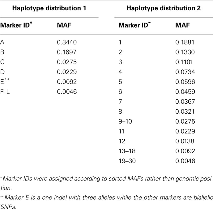
Table 1. Minor allele frequency (MAF) of markers resulting from sequencing data from the CHB sample of 1000 Genomes Project.

For Haplotype Distribution 1, case–control samples were generated assuming that 4 out of the 12 markers were causal. All combinations of four causal markers were considered in the simulation studies, resulting in 495 possible scenarios. Data was generated under four simulation settings in order to investigate the performance of genotype-level vs. similarity-level collapsing. (1) Under the first setting (Figure 1), all four causal loci increase the disease risk with the same odds ratio of 1.3. (2) Under the second setting (Figure 2), we allowed the four causal loci to have various effect sizes on the phenotype. Those with MAF less than 0.01 were set to have an odds ratio of 2 while all others were set to have an odds ratio of 1.3. (3) Under the third setting (Figure 3), we took advantage of the triallelic indel in the marker set and allowed two of three alleles from the indel to be causal (i.e., the rarest and second rarest, with frequencies 0.009 and 0.096 respectively). In this setting, we only considered scenarios where this indel was included as one of the four causal loci (which resulted in 165 possible scenarios instead of 495). Each causal variant was set to have the same effect on the phenotype with an odds ratio of 1.3. (4) Under the fourth setting (Figures 4–5), we considered different proportions of causal loci in the marker set – 2 out of 12 and 4 out of 4. In both scenarios, the causal loci were set to have the same effect on the phenotype with an odds ratio of 1.3. When 2 out of 12 loci were assumed to be causal, all combinations of two markers were considered, resulting in 66 possible scenarios. When four out of four loci were assumed to be causal, the same 495 possible scenarios were considered, but the remaining eight loci were not included in the marker set during the analysis.

FIGURE 1

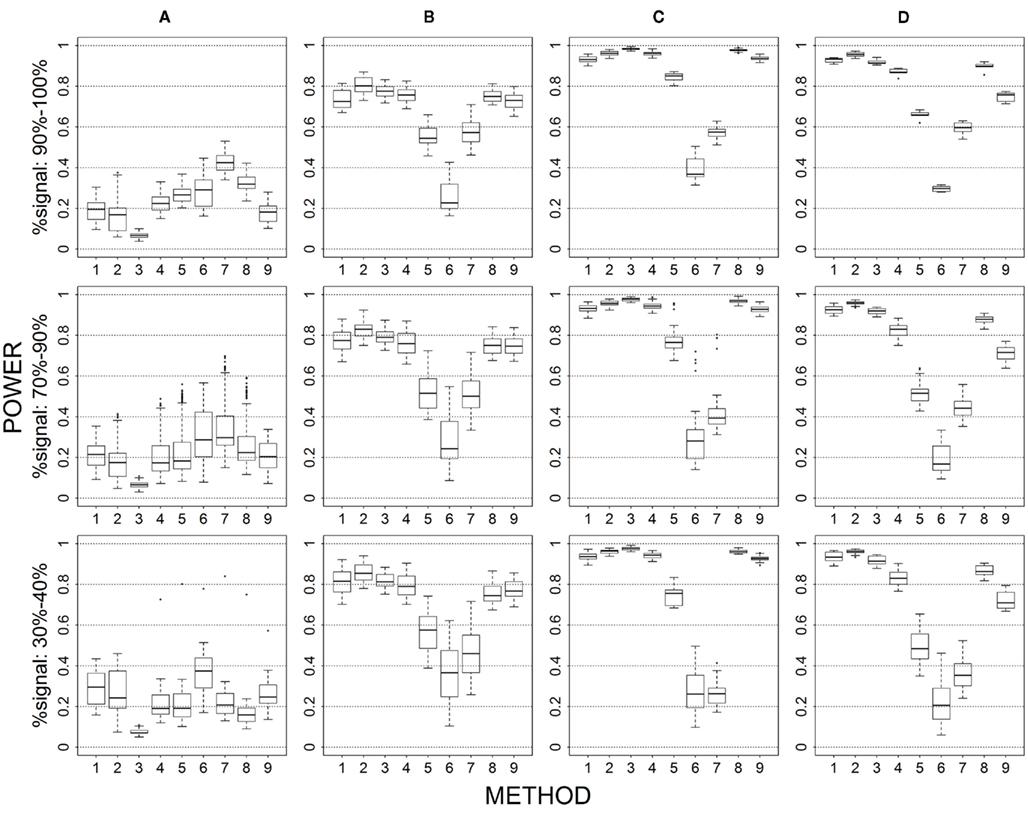
Figure 1. Power results when casual loci have same effects under 4 causal loci out of 12 markers setting for binary trait. Power is calculated over 500 replicate data sets with α = 0.05; there are 495 possible combinations of 4 causal loci out of 12 markers; boxplots summarize the power results for marker-combinations belonging to each average functional allele frequency [(A) is 0–0.02, (B) is 0.04–0.06, (C) is 0.08–0.11, (D) is 0.13–0.15] and percent-signal category; 1 = CMC01, 2 = CMC05, 3 = SimReg0, 4 = SimReg3, 5 = SimReg4, 6 = SKATsr, 7 = VT, 8 = 2Stage, 9 = MinP.

FIGURE 2

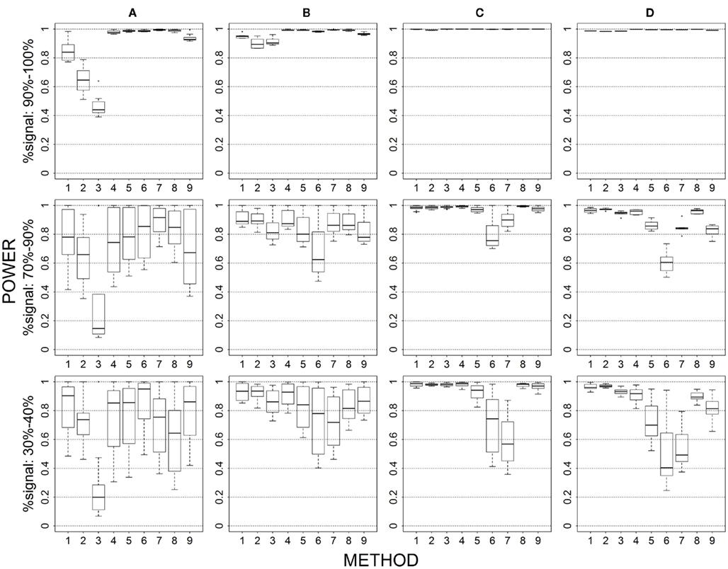
Figure 2. Power results when casual loci have different risk effect sizes under 4 causal loci out of 12 markers setting for binary trait. Power is calculated over 500 replicate data sets with α = 0.05; there are 495 possible combinations of 4 causal loci out of 12 markers; boxplots summarize the power results for marker-combinations belonging to each average functional allele frequency [(A) is 0–0.02, (B) is 0.04–0.06, (C) is 0.08–0.11, (D) is 0.13–0.15] and percent-signal category; 1 = CMC01, 2 = CMC05, 3 = SimReg0, 4 = SimReg3, 5 = SimReg4, 6 = SKATsr, 7 = VT, 8 = 2Stage, 9 = MinP.

FIGURE 3

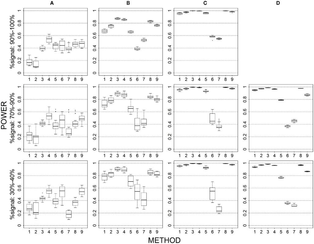
Figure 3. Power results for multiple causal alleles in a locus with same effects under 4 loci out of 12 markers setting for binary trait. Power is calculated over 500 replicate data sets with α = 0.05; there are 165 possible combinations of 4 causal loci out of 12 markers; boxplots summarize the power results for marker-combinations belonging to each average functional allele frequency [(A) is 0.02–0.06, (B) is 0.06–0.10, (C) is 0.10–0.14, (D) is 0.14–0.16] and percent-signal category; 1 = CMC01, 2 = CMC05, 3 = SimReg0, 4 = SimReg3, 5 = SimReg4, 6 = SKATsr, 7 = VT, 8 = 2Stage, 9 = MinP.

FIGURE 4

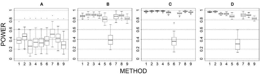
Figure 4. Power results when casual loci have same effects under 4 causal loci out of 4 markers setting for binary trait. Power is calculated over 500 replicate data sets with α = 0.05; there are 495 possible combinations of 4 causal loci out of 12 markers; boxplots summarize the power results for marker-combinations belonging to each average functional allele frequency [(A) is 0–0.02, (B) is 0.04–0.06, (C) is 0.08–0.11, (D) is 0.13–0.15] and percent-signal category; 1 = CMC01, 2 = CMC05, 3 = SimReg0, 4 = SimReg3, 5 = SimReg4, 6 = SKATsr, 7 = VT, 8 = 2Stage, 9 = MinP.

FIGURE 5

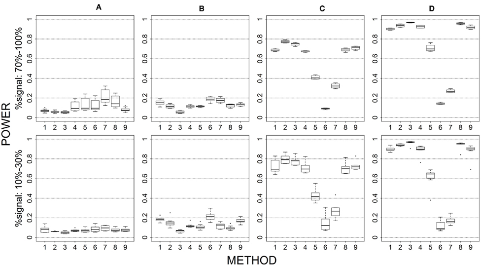
Figure 5. Power results when casual loci have same effects under 2 loci out of 12 markers setting for binary trait. Power is calculated over 500 replicate data sets with α = 0.05; there are 66 possible combinations of 2 causal loci out of 12 markers; boxplots summarize the power results for marker-combinations belonging to each average functional allele frequency [(A) is 0–0.01, (B) is 0.01–0.03, (C) is 0.08–0.10, (D) is 0.16–0.26] and percent-signal category; 1 = CMC01, 2 = CMC05, 3 = SimReg0, 4 = SimReg3, 5 = SimReg4, 6 = SKATsr, 7 = VT, 8 = 2Stage, 9 = MinP.

For Haplotype Distribution 2, case–control samples were generated assuming that 2 out of the 30 markers were causal. All combinations of two causal markers were considered in the simulation studies, resulting in 435 possible scenarios. Data was generated under two simulation settings in order to investigate the two collapsing paradigms’ performance in a larger genomic region with a low proportion of causal variants. (1) The first setting (Figure 6) is analogous to Setting 1 for Haplotype Distribution 1. That is, both causal loci were set to have the same effect size on the phenotype – an odds ratio of 1.3. (2) The second setting (Figure 7) is analogous to Setting 2 for Haplotype Distribution 1. That is, both causal loci were allowed to have different effect sizes with the same direction on the phenotype. When the MAF of the causal loci was less than 0.01, the odds ratio was taken to be 2; otherwise it was taken to be 1.3.

FIGURE 6

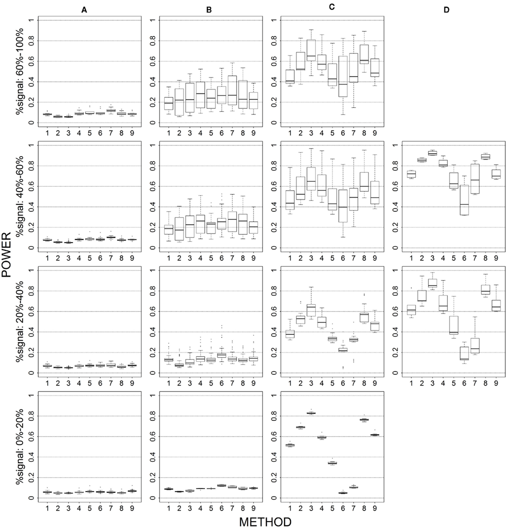
Figure 6. Power results when casual loci have same effects under 2 loci out of 30 markers setting for binary trait. Power is calculated over 500 replicate data sets with α = 0.05; there are 435 possible combinations of 2 causal loci out of 30 markers; boxplots summarize the power results for marker-combinations belonging to each average functional allele frequency [(A) is 0–0.01, (B) is 0.01–0.05, (C) is 0.05–0.10, (D) is 0.10–0.20] and percent-signal category; 1 = CMC01, 2 = CMC05, 3 = SimReg0, 4 = SimReg3, 5 = SimReg4, 6 = SKATsr, 7 = VT, 8 = 2Stage, 9 = MinP.

FIGURE 7

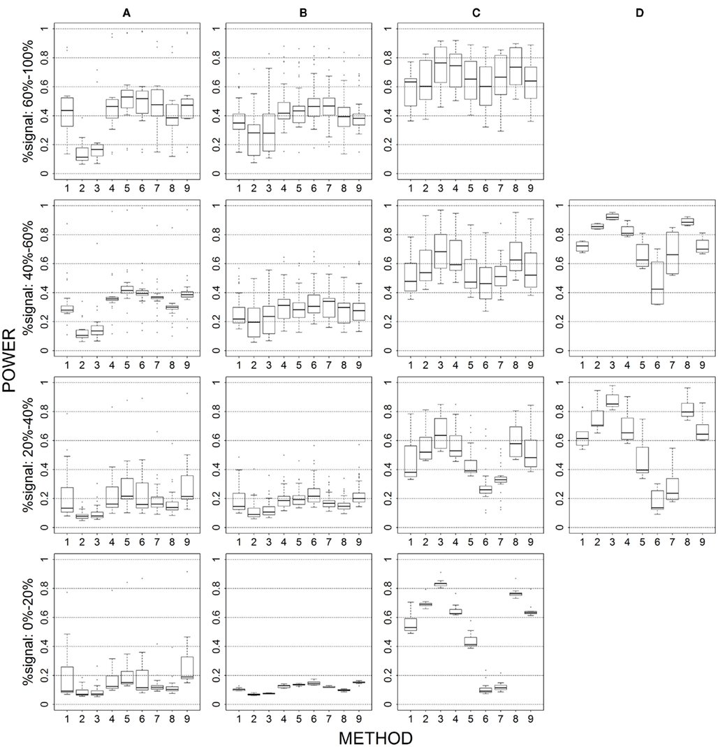
Figure 7. Power results when casual loci have different risk effect sizes under 2 loci out of 30 markers setting for binary trait. Power is calculated over 500 replicate data sets with α = 0.05; there are 435 possible combinations of 2 causal loci out of 30 markers; boxplots summarize the power results for marker-combinations belonging to each average functional allele frequency [(A) is 0–0.01, (B) is 0.01–0.05, (C) is 0.05–0.10, (D) is 0.10–0.20] and percent-signal category; 1 = CMC01, 2 = CMC05, 3 = SimReg0, 4 = SimReg3, 5 = SimReg4, 6 = SKATsr, 7 = VT, 8 = 2Stage, 9 = MinP.

Data generation

To create a case–control sample of size n under an additive genetic model, we generated the haplotype pair of an individual conditional on their disease status and then dissolved the haplotype pair into its unphased genotypes. Let P(H = h|Y = y) denote the probability of having a particular haplotype pair conditional on disease status. This probability can be expressed as

For a case individual, P(Y = 1|H = h) was found using the logistic regression model

For a control individual, P(Y = 0|H = h) = 1 − P(Y = 1|H = h). The function Z(·) depends on the genetic mode of the loci associated with the disease. Under an additive genetic model, Z(D) = D where D is the vector of minor allele counts for each locus in a given haplotype pair. The vector β was taken to be the log of 1.3 or 2 for all causal loci and the log of 1.0 for all non-causal loci in the marker set. The value of β₀ was set to maintain a disease prevalence of 1%. Once P(Y = y|H = h) was calculated for each haplotype pair formed from the derived haplotype distribution, the vectors P_(H|Y=y) = (P(H = h₁|Y = y)…P(H = h_q|Y = y)) were calculated for Y = 0 and Y = 1, where q is total number of haplotype pairs. The sample was generated by taking 1000 draws from the multinomial distribution parameterized by P_(H|Y=0) to determine the haplotype pairs of the control individuals and by taking 1000 draws from the multinomial distribution parameterized by P_(H|Y=1) to determine the haplotype pairs of the case individuals. The haplotype pair of each individual was then dissolved into its unphased genotype.

Computational details

For each simulation setting, 500 replicate data sets were generated for each possible combination of 4 (or 2) causal loci. Each data set was analyzed using the following methods: (1) MinP; (2) CMC with the MAF collapsing threshold set at 0.01 or 0.05, which will be referred to as CMC01 and CMC05, respectively; (3) VT; (4) SimRegX, i.e., SimReg based on all loci with weights taken to be f^−0/4 (SimReg0), f^−3/4 (SimReg3), and f^−4/4 (SimReg4); and (5) SKATsr, i.e., SimReg based on rare variants only by using the SKAT weight (1 − f)²⁴. In addition, we also considered a two-stage procedure that combines genotype-level collapsing and similarity-level collapsing. The two-stage procedure, referred to as 2stage, performs both SimReg0 and VT, but assesses the significance of each analysis at α/2 instead of α like the other methods, where α is a desired significance level. If either underlying method rejects the null hypothesis, the two-stage procedure rejects the null. The performance of each method was compared by calculating their power to detect the association between the marker set and the phenotype at α = 0.05 as well as their Type I error rate.

Results

To investigate the performance of each collapsing paradigm, we calculated each representative method’s Type I error rate and power to detect an informative marker set (i.e., one containing causal loci). We present the Type I error rates in Table 2. All methods have desirable and similar performances under a null model. Each had Type I error rates that were around the nominal level being considered (i.e., α = 0.01, 0.05, or 0.10). We present power results in Figures 1–8. Each figure groups the results into categories defined by combinations of two factors – range of average causal allele frequency (across columns) and range of percent-signal (down rows). Percent-signal is calculated as

where m is the total number of loci in the marker set, m_c is the number of causal loci in the marker set, m_nc = m − m_c is the number of non-causal loci, and is the average pair-wise between causal and non-casual loci for simulation scenario i. The quantities max and min are the maximum and minimum, respectively, of across all i. The fraction is used to rescale the small range of the observed to range from 0 and 1. Within each figure, boxplots of the power results (listed on the y-axis) are given for the methods under consideration (listed on the x-axis) for each category. Boxplots were created using the power results from the simulated marker-set scenarios that belonged to each average-causal allele frequency by percent-signal category.

TABLE 2

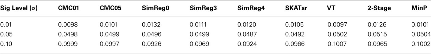
Table 2. Type I error rates averaged over the 495 possible scenarios for 4 causal markers out of 12 and 500 replicate data sets.

FIGURE 8

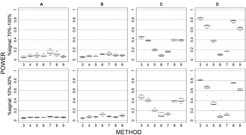
Figure 8. Power results when casual loci have same effects under 2 loci out of 12 markers setting for quantitative trait. Power is calculated over 500 replicate data sets with α = 0.05; there are 66 possible combinations of 2 causal loci out of 12 markers; boxplots summarize the power results for marker-combinations belonging to each average functional allele frequency [(A) is 0–0.01, (B) is 0.01–0.03, (C) is 0.08–0.10, (D) is 0.16–0.26] and percent-signal category; 3 = SimReg0, 4 = SimReg3, 5 = SimReg4, 6 = SKATsr, 7 = VT, 8 = 2Stage, 9 = MinP (Note: 1 = CMC01 and 2 = CMC05 are not applicable to quantitative traits).

Underlying Genetic Architecture

Causal allele frequency (Figures 1 and 6)

The average causal allele frequency reflects the ratio of rare causal variants to common causal variants in the analysis set. A low average causal allele frequency results from a high rare to common variant ratio, whereas a moderate or high average causal allele frequency results from a mix of rare and common variants or a low rare to common variant ratio. In Figures 1 and 6, geno-sum and sim-sum methods have comparable performances when comparing rare-variant approaches to rare-variant approaches and all-variant approaches to all-variant approaches. That is, VT and SKATsr have similar power when the causal allele frequencies are low. However, when the causal allele frequencies increase, VT performs slightly better than SKATsr. Similarly, CMC and SimRegX have similar power with the exception SimReg4 at moderate and high frequencies. In these settings, SimReg4 under performs compared to the other versions of SimRegX and tends to perform more like the rare-variant approaches as it most strongly upweights the contribution from rare variants. As expected, the relative performance between rare-variant and all-variant approaches depends on the underlying causal allele frequencies. When causal allele frequencies are low (i.e., Column 1), methods that target rare variants (i.e., VT and SKATsr) have the best performance. As the frequencies increase to moderate or high (i.e., Columns 2–4 in the Figure 1 and Columns 3–4 in Figure 6), methods that use all variants (i.e., CMC and SimRegX) start to outperform the rare-variant approaches. At these elevated causal allele frequencies, the power difference between rare-variant and all-variant approaches is more substantial for sim-sum methods (i.e., SKATsr vs. SimRegX) than for geno-sum methods (i.e., VT vs. CMC) as the power of SKATsr remains relatively constant as the frequencies increase. SKATsr does not take advantage of any information from common variants because it extremely downweights their contributions in the combined genotype. As a result, VT typically outperforms SKATsr when causal allele frequencies are high because it uses variable thresholding that can include common variants in the analysis. The two-stage procedure, which combines VT and SimReg0, does not suffer the same dramatic power switch when the causal allele frequencies change and is able to maintain similar or higher power than the best collapsing approach. MinP never uniformly outperforms or is outperformed by any geno-sum or sim-sum method. However, it often had satisfactory performance when the percent-signal is low (e.g., the bottom row in Figures 1, 3, 4, and 6). The above observations hold regardless of the percent-signal. When investigating the impact of other simulation factors, we will refer back to this scenario as a baseline for comparison.

Magnitude of causal allele effect (Figures 2 vs. 1 and 7 vs. 6)

When we allow the underlying causal variants to have different effects sizes in the same direction, we see an overall increase in power for all methods. The largest gain in power is seen for rare-variant sim-sum approaches, as seen in SKATsr which shortens its gap with VT or even has better power when, e.g., comparing Figure 2 to Figure 1. Substantial power gain is also observed for all-variant sim-sum methods at low causal allele frequencies, where SimReg3 and SimReg4 have comparable or better power than VT and SKATsr. Nevertheless, the general pattern of results observed in the baseline scenario still holds. That is, geno-sum and sim-sum methods have comparable performances when comparing similar approaches (i.e., rare-variant to rare-variant, similarly for all-variant approaches) across all simulation settings.

Multiple causal alleles in a locus (Figures 3 vs. 1)

When we allow multiple alleles within a locus to be causal with the same effect, sim-sum methods generally perform better than geno-sum methods. That is, SimReg3 is the best or near-best across all simulation settings. When comparing rare-variant approaches, SKATsr performs better than VT at low frequencies and becomes comparable to VT when the frequencies increase (i.e., no longer have power loss). This result is different from the baseline scenario where SKATsr is comparable to VT when frequencies are low and tends to have less power as frequencies increase. Similarly, when comparing all-variant approaches, SimRegX outperforms CMC, with the exception of SimReg4, regardless of the underlying causal allele frequencies. These patterns hold regardless of percent-signal.

Composition of Marker Set

Proportion of causal Loci (Figures 1, 4, 5, and 6)

Results of different proportions of causal loci are shown in Figure 4 (for 4 out of 4), Figure 1 (for 4 out of 12), Figure 5 (for 2 out of 12), and Figure 6 (for 2 out of 30). When the proportion of causal loci is high (4/4 scenario; Figure 4), geno-sum performs better than or similar to sim-sum across different settings. Specifically, for all-variant methods (i.e., CMC vs. SimRegX), geno-sum and sim-sum methods generally perform comparably, and at low causal allele frequencies, geno-sum has a slight advantage over sim-sum. For rare-variant methods (i.e., VT vs. SKATsr), geno-sum clearly outperforms sim-sum. Furthermore, VT performs comparable to SimRegX even at moderate and high causal allele frequencies.

When the proportion of causal loci drops, all methods suffer a power loss, but the loss suffered by sim-sum is less than that suffered by geno-sum. As a result, sim-sum begins to have similar or more power than its geno-sum counterpart. For example, if we focus on low causal alleles frequencies (i.e., first column), we see that the power gain of VT over SKATsr becomes smaller and smaller when we move from Figure 4 (4/4), to Figure 1 (4/12), to Figure 5 (2/12) and to Figure 6 (2/30). Additionally, when percent-signal is low, SKATsr can outperform VT. The relative performance of the two-stage procedure remains consistent regardless of the proportion of causal loci. That is, the power of 2stage always falls between that of VT and SimReg0, and thus outperforms the SimReg0 at low causal allele frequency when VT is superior and vice versa when the causal allele frequency is moderate or high.

LD between causal and non-causal loci (Figure 1)

Recall that the calculation of percent-signal involves two components: (1) R² that reflects the LD between causal and non-causal loci in the marker set, and (2) the proportional of causal loci. As such, percent-signal can be used as a proxy to investigate the effects of the underlying LD on the paradigms’ performances. All methods suffer a power loss as LD decreases (i.e., Figure 1, from top row to bottom row), but sim-sum is less sensitive to the decrease of LD compared to geno-sum. Therefore, although general trends among the methods’ performances hold regardless of the underlying LD, the magnitude of the power gain or loss between the geno-sum and sim-sum methods is influenced by changes in LD. For rare-variant approaches, SKATsr is quite robust to the decrease of LD, while VT is sensitive to the drop of LD and decreases with LD. As a result, when the causal allele frequencies are low, the relative performance of SKATsr vs. VT flip-flops depending on LD (i.e., Column 1 in Figure 1). For moderate or high allele frequencies, the relative power loss of SKATsr compared to VT increases as LD increases. Because SKATsr does not incorporate information from common variants, it cannot fully benefit from an increase in LD like VT whose power increases with LD as it is able to incorporate information from common variants (i.e., Figures 1, 5, and 6). For all-variant approaches, SimRegX and CMC are fairly robust to LD changes and their performances remain comparable as LD changes, with the exception of SimReg4. CMC is a hybrid of a geno-sum approach and a classic genotype-based multimarker approach; therefore it is not as sensitive to the underlying LD pattern like typical geno-sum approaches such as VT. The power of the two-stage procedure is also fairly robust to changes in LD.

Weighting Schemes Used in Collapsing Methods

SimReg method

SimReg0, SimReg3 vs. SimReg4. For sim-sum methods based on all loci, when the causal allele frequencies are low, SimReg0, which does not upweight contributions from rare alleles, has the lowest power, and SimReg4, which uses the strongest weights to promote sharing from rare alleles, has the highest power. And as expected, when the causal allele frequencies increase, the relationship flips. This pattern of results holds regardless of percent-signal. However, the pattern does not hold when multiple alleles within a particular locus are causal (Figure 3). Under this scenario, SimReg4 no longer outperforms the other versions of SimRegX at low causal allele frequencies; instead SimReg3 performs the best. Overall, the results show that using strong weights can boost the power to detect rare variants, but it may risk losing power when some causal variants are common. Among the weights studied, SimReg3 appears to achieve a better compromise and exhibited more robustness against the influence of causal allele frequencies.

Rare variants vs. all variants. When the causal loci are rare, the results suggest that SimReg4 is not strong enough to surpass VT and more extreme weights such as SKAT weights are needed. At low causal allele frequencies, SKATsr outperforms SimReg4, and SimReg4 performs comparably to SimReg3 which outperforms SimReg0. As the causal allele frequencies increase, SKATsr and SimReg4 suffer a power loss, which is quite severe for SKATsr. This again suggests that it might be advantageous to use a sim-sum method that considers all variants with a moderate weighting scheme (e.g., SimReg3), since it achieves better power at moderate and high causal allele frequencies, and yet the power loss at low causal allele frequencies is not as severe as the power loss observed for SKATsr at moderate and high causal allele frequencies.

CMC method

Like SimReg, which version of CMC performs the best appears to depend on the frequency of the causal alleles in the marker set (see Figures 1–3). When the causal allele frequencies are low, CMC01 performs better than CMC05. However, when the causal allele frequencies are moderate or high, CMC05 performs better than CMC01. This pattern holds regardless of percent-signal, the magnitude of the causal effect, or the number of causal alleles at a particular locus. These results suggest using a fixed threshold in geno-sum methods may be unsatisfactory. When the threshold is set too low, the power of CMC may suffer due to increased degrees of freedom. However, if the threshold is set too high, the power of CMC may also suffer as noise loci are introduced into the combined genotype.

VT method

The weighting scheme of VT is to triage loci with high MAF. It weights each locus by an indicator function, i.e., weight equal to 1 if MAF is less than a data-driven threshold T, and weight equal to 0 otherwise. As a result, it performed the best if all causal alleles have small frequencies. It suffered non-trivial power loss if some heterogeneity existed among allele frequencies. Nevertheless, compared to other approaches that target rare variants (e.g., SKATsr), the advantage of a data-driven threshold becomes apparent when non-rare variants are present in the marker set: The power loss between VT and its all-variant counterpart is significantly less severe than that of SKATsr. VT’s adaptive threshold permits the inclusion of some information from common variants, while SKATsr’s strong weight against common variants does not allow them to contribute any information to the combined genotype.

Discussion

Collapsing methods are drawing big attention due to their usefulness in marker-set analysis and rare variant detection. Collapsing information can be done at genotype level or at similarity level.

In this work, we investigated the implications of employing these different collapsing strategies when performing multimarker association analysis in order to uncover the strengths and weaknesses of the two paradigms. Using realistic data based on 1000 Genomes Project, we considered scenarios where the causal alleles can be rare, non-rare, or a mixture of two, where the causal loci can be biallelic SNPs or multiallelic markers, and where the association signal of a marker set, quantified based on the proportion of causal loci and LD structure, varied from weak to strong. We also considered approaches proposed to better target rare variants and those that use all variant information in the marker set. For genotype-level collapsing, we considered VT, which aggregates and uses information only from loci with MAF below the adaptive threshold, and CMC, which collapses rare-variant information but retains and analyzes information from all loci. For similarity-level collapsing, we considered SimReg which can incorporate many current variance-component based approaches (e.g., C-alpha and SKAT) as special cases. As a result, SimReg can be used as a rare-variant as well as an all-variant approach. We considered weights that upweighted the contribution from rare variants with varying strengths, ranging from the extreme case that placed almost no weight on common variants (SKATsr), to strong-but-not-extreme weights against common variants (SimReg4 and SimReg3), to not promoting rare variants at all (SimReg0).

Our results show that neither collapsing strategy outperforms the other across all simulated scenarios. Nevertheless, employing a collapsing strategy is advantageous across all simulated scenarios. At least one of the two strategies resulted in higher power than the standard approach which does not aggregate information across markers. Two factors that dominate the performance of the collapsing strategies are the signal-to-noise ratio and the underlying genetic architecture of the causal variants. We found that similarity-level collapsing tends to be more robust to changes in the signal-to-noise ratio. That is, the power loss due to the inclusion of non-causal variants in the marker was much less substantial for similarity-level collapsing than for genotype-level collapsing. This can be seen by comparing the power loss from Figure 4 (i.e., 4 out of 4) to Figure 1 (4 out of 12), Figure 5 (2 out of 12), and Figure 6 (2 out of 30), as well as the similar or higher power of similarity collapsing than genotype collapsing when the proportion of the functional loci is moderate or low (e.g., Figures 5–7).

The performance of these collapsing strategies was also heavily influenced by the underlying genetic architecture of the causal variants, which we refer to as their effect patterns (e.g., same or varying effect sizes/directions, linear vs. non-linear, additive vs. interactive) and the variant frequencies. Genotype-level collapsing generally performs best when the genetic architecture of the causal variants is not complex. That is, the causal variants have similar, additive, linear effects with similar frequencies. When collapsing at the genotype level, the underlying philosophy is that all loci share the same effect size (and hence can be well detected by a common regression coefficient). Therefore the approach lends itself to scenarios where the proportion of functional loci in a marker set is high and each locus exhibits similar influence on traits. In contrast, collapsing at the similarity level can be viewed as test of the variation among regression coefficients and allows each locus to have a different effect size. As a result, this approach can accommodate more complex genetic architectures such as a mixture of rare and non-rare variants, different effect sizes and directions, and multiple causal alleles within a locus. This notion is supported by our results which show that similarity-level collapsing is more robust as the complexity of the genetic architecture increases and outperforms genotype collapsing when the genetic architecture of the marker set becomes more sophisticated.

The underlying causal allele frequencies impact the choice of the weighting scheme (i.e., approaches based on all variants vs. rare variants only) more than the choice of collapsing paradigm. As expected, when the causal variants are rare, approaches that target rare variants will be the best, but when there is a mixture of rare and common, approaches that use all variant information will be the best. The power lost by using a rare-variant approach when common causal variants are present in the marker set is much more severe than the power lost by using an all-variant approach when the causal variants are all rare. Based on this observation and because the frequency of causal variants is not known a priori, a reasonable strategy would be to use an all-variant approach with a moderate weight against common variants, such as SimReg3 or CMC with a suitable threshold. Indeed, our results also show that using an adaptive threshold can gain robustness against the unknown frequency distributions of the causal variants (i.e., the relatively small power loss of VT compared to SKATsr for high allele frequencies). This suggests that CMC with variable threshold holds good potential.

Because the optimal statistical methods depend on the unknown architecture of the causal variants and the marker set, we also considered a two-stage analysis. The two-stage procedure performs both VT, which generally performs the best for rare variants, and SimReg0, which generally performs the best or near-best for common variants. Like CMC, this hybrid strategy uses two different strategies to detect rare and non-rare variants. However the two-stage approach can gain efficiency by using fewer degrees of freedom when modeling multiple common variants and is applicable to quantitative traits. By combining the top method from each scenario, the two-stage approach is reasonably robust and yields comparable though not necessarily the highest power across all simulation scenarios. It provides an attractive alternative to SimReg3 and CMC with variable threshold.

We focused on binary phenotypes in our simulation studies. However, most of the methods considered here are applicable to quantitative phenotypes (except CMC). We simulated data under one setting (2 causal loci out of 12 markers with same effects; see Figure 8) to compare the performance of these methods for binary and quantitative traits. The general pattern of our findings typically holds between the two trait types. In short, genotype collapsing is more sensitive to the marker set being contaminated by noise loci than similarity collapsing. In addition, genotype collapsing performs best when the genetic architecture of the marker set is not complex (e.g., causal loci with similar effects and similar frequencies). Similarity collapsing is more robust as the complexity of the genetic architecture increases and outperforms genotype collapsing when the genetic architecture of the marker set becomes more sophisticated (e.g., causal loci with various effect sizes or frequencies and potential non-linear or interactive effects). We expect the same trends of results to occur under the other simulation settings.

Conflict of Interest Statement

The authors declare that the research was conducted in the absence of any commercial or financial relationships that could be construed as a potential conflict of interest.

Acknowledgments

This work was supported by National Institutes of Health grants R01 MH074027 and P01 CA142538.

References

Bacanu, S. A., Nelson, M. R., and Whittaker, J. C. (2011). Comparison of methods and sampling designs to test for association between rare variants and quantitative traits. Genet. Epidemiol. 35, 226–235.

Ballard, D. H., Cho, J., and Zhao, H. (2010). Comparisons of multi-marker association methods to detect association between a candidate region and disease. Genet. Epidemiol. 34, 201–212.

Pubmed Abstract | Pubmed Full Text | CrossRef Full Text

Bansal, V., Libiger, O., Torkamani, A., and Schork, N. J. (2010). Statistical analysis strategies for association studies involving rare variants. Nat. Rev. Genet. 11, 773–785.

Pubmed Abstract | Pubmed Full Text | CrossRef Full Text

Basu, S., and Pan, W. (2011). Comparison of statistical tests for disease association with rare variants. Genet. Epidemiol. 35, 606–619.

Pubmed Abstract | Pubmed Full Text | CrossRef Full Text

Browning, S. R., and Browning, B. L. (2007). Rapid and accurate haplotype phasing and missing-data inference for whole-genome association studies by use of localized haplotype clustering. Am. J. Hum. Genet. 81, 1084–1097.

Pubmed Abstract | Pubmed Full Text | CrossRef Full Text

Chapman, J., and Whittaker, J. (2008). Analysis of multiple SNPs in a candidate gene or region. Genet. Epidemiol. 32, 560–566.

Pubmed Abstract | Pubmed Full Text | CrossRef Full Text

DePristo, M. A., Banks, E., Poplin, R., Garimella, K. V., Maguire, J. R., Hartl, C., Philippakis, A. A., del Angel, G., Rivas, M. A., Hanna, M., McKenna, A., Fennell, T. J., Kernytsky, A. M., Sivachenko, A. Y., Cibulskis, K., Gabriel, S. B., Altshuler, D., and Daly, M. J. (2011). A framework for variation discovery and genotyping using next-generation DNA sequencing data. Nat. Genet. 43, 491–498.

Pubmed Abstract | Pubmed Full Text | CrossRef Full Text

Gauderman, W. J., Murcray, C., Gilliland, F., and Conti, D. V. (2007). Testing association between disease and multiple SNPs in a candidate gene. Genet. Epidemiol. 31, 383–395.

Pubmed Abstract | Pubmed Full Text | CrossRef Full Text

Goeman, J. J., van de Geer, S. A., de Kort, F., and van Houwelingen, H. C. (2004). A global test for groups of genes: testing association with a clinical outcome. Bioinformatics 20, 93–99.

Pubmed Abstract | Pubmed Full Text | CrossRef Full Text

Han, F., and Pan, W. (2010). A data-adaptive sum test for disease association with multiple common or rare variants. Hum. Hered. 70, 42–54.

Pubmed Abstract | Pubmed Full Text | CrossRef Full Text

Hoffmann, T. J., Marini, N. J., and Witte, J. S. (2010). Comprehensive approach to analyzing rare genetic variants. PLoS ONE 5, e13584. doi:10.1371/journal.pone.0013584

Pubmed Abstract | Pubmed Full Text | CrossRef Full Text

Ionita-Laza, I., Buxbaum, J. D., Laird, N. M., and Lange, C. (2011). A new testing strategy to identify rare variants with either risk or protective effect on disease. PLoS Genet. 7, e1001289. doi:10.1371/journal.pgen.1001289

Pubmed Abstract | Pubmed Full Text | CrossRef Full Text

Kwee, L. C., Liu, D., Lin, X., Ghosh, D., and Epstein, M. P. (2008). A powerful and flexible multilocus association test for quantitative traits. Am. J. Hum. Genet. 82, 386–397.

Pubmed Abstract | Pubmed Full Text | CrossRef Full Text

Li, B., and Leal, S. M. (2008). Methods for detecting associations with rare variants for common diseases: application to analysis of sequence data. Am. J. Hum. Genet. 83, 311–321.

Pubmed Abstract | Pubmed Full Text | CrossRef Full Text

Li, M., Wang, K., Grant, S. F. A., Hakonarson, H., and Li, C. (2009). ATOM: a powerful gene-based association test by combining optimally weighted markers. Bioinformatics 25, 497–503.

Pubmed Abstract | Pubmed Full Text | CrossRef Full Text

Lin, D. Y., and Tang, Z. Z. (2011). A general framework for detecting disease associations with rare variants in sequencing studies. Am. J. Hum. Genet. 89, 354–367.

Pubmed Abstract | Pubmed Full Text | CrossRef Full Text

Lin, W. Y., and Schaid, D. J. (2009). Power comparisons between similarity-based multilocus association methods, logistic regression, and score tests for haplotypes. Genet. Epidemiol. 33, 183–197.

Pubmed Abstract | Pubmed Full Text | CrossRef Full Text

Madsen, B. E., and Browning, S. R. (2009). A groupwise association test for rare mutations using a weighted sum statistic. PLoS Genet. 5, e1000384. doi:10.1371/journal.pgen.1000384

Pubmed Abstract | Pubmed Full Text | CrossRef Full Text

McKenna, A., Hanna, M., Banks, E., Sivachenko, A., Cibulskis, K., Kernytsky, A., Garimella, K., Altshuler, D., Gabriel, S., Daly, M., and DePristo, M. A. (2010). The genome analysis toolkit: a MapReduce framework for analyzing next-generation DNA sequencing data. Genome Res. 20, 1297–1303.

Pubmed Abstract | Pubmed Full Text | CrossRef Full Text

Morris, A. P., and Zeggini, E. (2010). An evaluation of statistical approaches to rare variant analysis in genetic association studies. Genet. Epidemiol. 34, 188–193.

Pubmed Abstract | Pubmed Full Text | CrossRef Full Text

Mukhopadhyay, I., Feingold, E., Weeks, D. E., and Thalamuthu, A. (2010). Association tests using kernel-based measures of multi-locus genotype similarity between individuals. Genet. Epidemiol. 34, 213–221.

Pubmed Abstract | Pubmed Full Text

Neale, B. M., Rivas, M. A., Voight, B. F., Altshuler, D., Devlin, B., Orho-Melander, M., Kathiresan, S., Purcell, S. M., Roeder, K., and Daly, M. J. (2011). Testing for an unusual distribution of rare variants. PLoS Genet. 5, e1001322. doi:10.1371/journal.pgen.1001322

CrossRef Full Text

Price, A. L., Kryukov, G. V., de Bakker, P. I. W., Purcell, S. M., Staples, J., Wei, L. J., and Sunyaev, S. R. (2010). Pooled association tests for rare variants in exon-resequencing studies. Am. J. Hum. Genet. 86, 832–838.

Pubmed Abstract | Pubmed Full Text | CrossRef Full Text

Schaid, D. J. (2010a). Genomic similarity and kernel methods I: advancements by building on mathematical and statistical foundations. Hum. Hered. 70, 109–131.

CrossRef Full Text

Schaid, D. J. (2010b). Genomic similarity and kernel methods II: methods for genomic information. Hum. Hered. 70, 132–140.

CrossRef Full Text

The 1000 Genomes Project Consortium. (2010). A map of human genome variation from population-scale sequencing. Nature 467, 1061–1073.

Pubmed Abstract | Pubmed Full Text | CrossRef Full Text

Tzeng, J. Y., and Zhang, D. (2007). Haplotype-based association analysis via variance component score test. Am. J. Hum. Genet. 81, 927–938.

Pubmed Abstract | Pubmed Full Text | CrossRef Full Text

Tzeng, J. Y., Zhang, D., Chang, S. M., Thomas, D. C., and Davidian, M. (2009). Gene-trait similarity regression for multimarker-based association analysis. Biomertrics 65, 822–832.

CrossRef Full Text

Tzeng, J. Y., Zhang, D., Pongpanich, M., Smith, C., McCarthy, M. I., Sale, M. M., Worrall, B. B., Hsu, F. C., Thomas, D. C., and Sullivan, P. F. (2011). Studying gene and gene-environment effects of uncommon and common variants on continuous traits: a marker-set approach using gene-trait similarity regression. Am. J. Hum. Genet. 89, 277–288.

Pubmed Abstract | Pubmed Full Text | CrossRef Full Text

Wang, K., and Abbott, D. (2008). A principal components regression approach to multilocus genetic association studies. Genet. Epidemiol. 32, 108–118.

Pubmed Abstract | Pubmed Full Text | CrossRef Full Text

Wang, T., and Elston, R. C. (2007). Improved power by use of a weighted score test for linkage disequilibrium mapping. Am. J. Hum. Genet. 80, 353–360.

Pubmed Abstract | Pubmed Full Text | CrossRef Full Text

Wessel, J., and Schork, N. J. (2006). Generalized genomic distance–based regression methodology for multilocus association analysis. Am. J. Hum. Genet. 79, 792–806.

Pubmed Abstract | Pubmed Full Text | CrossRef Full Text

Wu, M. C., Kraft, P., Epstein, M. P., Taylor, D. M., Chanock, S. J., Hunter, D. J., and Lin, X. (2010). Powerful SNP-set analysis for case-control genome-wide association studies. Am. J. Hum. Genet. 86, 929–942.

Pubmed Abstract | Pubmed Full Text | CrossRef Full Text

Wu, M. C., Lee, S., Cai, T., Li, Y., Boehnke, M., and Lin, X. (2011). Rare-variant association testing for sequencing data with the sequence kernel association test. Am. J. Hum. Genet. 89, 82–93.

Pubmed Abstract | Pubmed Full Text | CrossRef Full Text

Xiong, M., Zhao, J., and Boerwinkle, E. (2002). Generalized T2 test for genome association studies. Am. J. Hum. Genet. 70, 1257–1268.

Pubmed Abstract | Pubmed Full Text | CrossRef Full Text

Zhang, L., Pei, Y. F., Li, J., Papasian, C. J., and Deng, H. W. (2010). Efficient utilization of rare variants for detection of disease-related genomic regions. PLoS ONE 5, e14288. doi:10.1371/journal.pone.0014288

Pubmed Abstract | Pubmed Full Text | CrossRef Full Text