 Benito A. González1,2
 Juan P. Vásquez3,4
 Daniel Gómez-Uchida4,5
 Jorge Cortés3,4
 Romina Rivera3,6
 Nicolas Aravena3
 Ana M. Chero3Ana M. Agapito3
 Valeria Varas7
 Jane C. Wheleer2,8
 Pablo Orozco-terWengel9*
 Juan Carlos Marín3*
- 1Laboratorio de Ecología de Vida Silvestre, Facultad de Ciencias Forestales y de la Conservación de la Naturaleza, Universidad de Chile, Santiago, Chile
- 2South American Camelid Specialist Group, Survival Species Commission, International Union for Conservation of Nature, Santiago, Chile
- 3Laboratorio de Genómica y Biodiversidad, Departamento de Ciencias Básicas, Facultad de Ciencias, Universidad del Bío-Bío, Chillán, Chile
- 4GEECLAB, Departamento de Zoología, Facultad de Ciencias Naturales y Oceanográficas, Universidad de Concepción, Concepción, Chile
- 5Núcleo Milenio INVASAL, Concepción, Chile
- 6Departamento de Ciencias Básicas, Facultad de Ciencias, Universidad Santo Tomás, Iquique, Chile
- 7Doctorado en Ciencias, Mencioìn Ecologiìa y Evolucioìn, Instituto de Ciencias Ambientales and Evolutivas, Facultad de Ciencias, Universidad Austral de Chile, Valdivia, Chile
- 8CONOPA-Instituto de Investigación y Desarrollo de Camélidos Sudamericanos, Lima, Peru
- 9School of Biosciences, College of Biomedical and Life Sciences, Cardiff University, Cardiff, United Kingdom
The vicuña (Vicugna vicugna) is the most representative wild ungulate of the high Andes of South America with two recognized morphological subspecies, V. v. mensalis in the north and V. v. vicugna in the south of its distribution. Current vicuña population size (460,000–520,000 animals) is the result of population recovery programs established in response to 500 years of overexploitation. Despite the vicuña’s ecosystemic, economic and social importance, studies about their genetic variation and history are limited and geographically restricted. Here, we present a comprehensive assessment of the genetic diversity of vicuña based on samples collected throughout its distribution range corresponding to eleven localities in Peru and five in Chile representing V. v. mensalis, plus four localities each in Argentina and Chile representing V. v. vicugna. Analysis of mitochondrial DNA and microsatellite markers show contrasting results regarding differentiation between the two vicuña types with mitochondrial haplotypes supporting subspecies differentiation, albeit with only a few mutational steps separating the two subspecies. In contrast, microsatellite markers show that vicuña genetic variation is best explained as an isolation by distance pattern where populations on opposite ends of the distribution present different allelic compositions, but the intermediate populations present a variety of alleles shared by both extreme forms. Demographic characterization of the species evidenced a simultaneous and strong reduction in the effective population size in all localities supporting the existence of a unique, large ancestral population (effective size ∼50,000 individuals) as recently as the mid-Holocene. Furthermore, the genetic variation observed across all localities is better explained by a model of gene flow interconnecting them rather than only by genetic drift. Consequently, we propose space “continuous” Management Units for vicuña as populations exhibit differentiation by distance and spatial autocorrelation linked to sex biased dispersal instead of population fragmentation or geographical barriers across the distribution.
Introduction
The vicuña (Vicugna vicugna) is the most representative wild ungulate of the Andean high plateau in South America (Franklin, 1983; Wheeler, 1995, 2012). Its current distribution is limited to extreme altitude environments, living in arid landscapes with intense solar radiation and a hypoxic atmosphere (Franklin, 1982). Two morphological subspecies have been described, with geographical and habitat differences and supported by mitochondrial DNA markers (Marín et al., 2007a,b; Casey et al., 2018) the northern vicuña (V. v. mensalis) and the southern vicuña (V. v. vicugna). The subspecies mensalis, inhabits the ‘moist puna,’ is smaller and darker than the southern vicuña and is distinguished primarily by the long growth of hair on the chest (Wheeler, 2012). In contrast, the subspecies vicugna inhabits ‘dry puna’ within the Dry Diagonal belt (24° and 29° S; Ammann et al., 2001; Kull et al., 2002), lacks the long chest hairs, and has a lighter beige pelage coloration with white covering a greater portion of the body, rising halfway up the sides to mid-rib height and all the way to the ileum crest (Wheeler, 2012). Finally, the greater length of the southern vicuña molar line supports phenotypic differentiation (Wheeler and Laker, 2009). This division into two groups is further supported by the presence of two mitochondrial lineages differentiating each subspecies (Marín et al., 2017), with the southern subspecies showing greater haplotypic diversity than the northern one (Marín et al., 2007b). The biogeographical barrier between the subspecies has been suggested to correspond to the deep valley of Tarapaca in Chile (19°S) on the western side of the vicuña distribution, however, there is no evident barrier at a similar latitude on the eastern side (Bolivia) of the species distribution range (Wallace et al., 2010). Current vicuña distribution covers an area of 300,000 km2 with several populations having increased their numbers after a drastic historic reduction (Acebes et al., 2018). Distribution is limited to altitudes from ∼3,000 to ∼5,000 m above sea level (Baigún et al., 2008; Villalba et al., 2010) along a 2,600 km stretch of the Central High Andes between 9° 30′ S in Ancash, Peru, and 27° 31′ S in the San Guillermo Reserve, Argentina (Wheeler and Laker, 2009). During the 1980s Chile, Peru, and Bolivia donated vicuña to Ecuador which were introduced to Chimborazo National Park (1° 31′ S, 78° 51′ W) and currently represent a stable, growing population (Rodriìguez and Morales-Delanuez, 2017; Vicuña Convention, 2017). This population should not be considered part of the natural vicuña distribution as there is no sound evidence that the species previously existed in Ecuador.
Current vicuña distribution and abundance is the result of population recovery programs established in response to 500 years of overexploitation (Yacobaccio, 2009) and near extinction in the 1960s (Wheeler and Laker, 2009). At the time of lowest population size only 6,000–10,000 vicuñas were left, widely distributed in low density, highly dispersed populations, with some small groups persisting at the species’ southern distribution range (Grimwood, 1969; Boswall, 1972; Jungius, 1972). Thanks to the establishment of national parks and reserves, the Andean Vicuña Convention agreement, and funds from international NGOs, the vicuña population notably increased to over 200,000 individuals in four decades (Wheeler, 2006), with the northern populations showing greater recovery than the southern ones (Wheeler and Laker, 2009). Currently, a total population about 460,000–520,000 individuals inhabit the Andean high plateau (Vicuña Convention, 2017; Acebes et al., 2018), corresponding to a 50-fold increase in five decades of intensive protection and management.
Studies of vicuña genetics are limited and geographically restricted. Genetic structure has been determined using both nuclear and mitochondrial DNA in Peruvian localities (Wheeler et al., 2001), the north of Chile and Bolivia (Sarno et al., 2004), and north-western Argentina (Anello et al., 2016). The results of these studies have been used to identify four discrete Management Units (MUs; Wheeler et al., 2001; Casey et al., 2018) for the maintenance of locally adapted populations in Peru. MUs are defined as demographically independent populations whose dynamics depend on local birth and death rates rather than immigration from other populations (Taylor and Dizon, 1999). Although several researchers have advocated the use of MUs (e.g., Mosa, 1987; Marín et al., 2013b; Moodley et al., 2017), this approach has not been used for the vicuña despite its ecological, cultural and conservation importance (Wheeler et al., 2001; Sarno et al., 2004). Practical aspects deriving from the implementation of such classification would facilitate determination of the origin of skin and fiber from confiscated illegally hunted and trafficked materials (González et al., 2016), as has been done for other species (Moodley et al., 2017). Additionally, a thorough characterization of the vicuña genetic variation would facilitate comparison between the genetic diversity of wild populations and managed, captive production groups (Stølen et al., 2009; Escalante et al., 2014; Anello et al., 2016).
Here, we present a comprehensive assessment of the molecular diversity of vicuña based on samples collected throughout its distribution range. We analyze their genetic variation using 15 microsatellite loci and sequences of the left domain of the mitochondrial control region. We present evidence of (1) range-wide phylogeographic structure linked with vicuña evolutionary history; (2) patterns of molecular genetic structure among vicuñas; and (3) links between patterns of genetic variation with phylogeographic history and barriers to gene flow. We further utilize this evidence to (4) describe and contrast the evolutionary history and patterns of gene flow among these populations in order to propose effective MUs for the species at broad scale.
Materials and Methods
Ethics Statement
Samples were collected throughout the current distributional range of the vicuña (Table 1 and Figure 1) following guidelines of the American Society of Mammalogists (Sikes et al., 2011). Specific permits were required for the Servicio Agrícola y Ganadero, SAG (permit 447, 2002), the Corporación Nacional Forestal, CONAF (permit 6/02, 2002), for granting other collection permits and helping in collecting samples. The animal research oversight committee of Universidad del Bío-Bío had knowledge of sampling plans prior to their approval of the present animal research protocol. All experimental protocols were approved by the Institutional Animal Care and Use Committee of Universidad del Bío-Bío, the methods were carried out in accordance with the approved guidelines. Samples were collected and exported for analysis (CITES permits 6282, 4222, 6007, 5971, 0005177, 0005178, 023355, 022967, and 022920) and imported to the United Kingdom (permits 269602/01, 262547/02). Peruvian samples were collected under permits from CONACS (28 September 1994, 15 June 1997), INRENA (011-c/c-2004-INRENA-IANP; 012-c/c-2004-INRENA-IANP; 016-c/c-2004-INRENA-IFFS-DCB; 016-c/c-2004-INRENA-IFFS-DCB; 021-c/c-2004-INRENA-IFFS-DCB; 026-c/c-2005-INRENA-IANP) and DGFFS (109-2009-AG-DGFFS-DGEFFS).
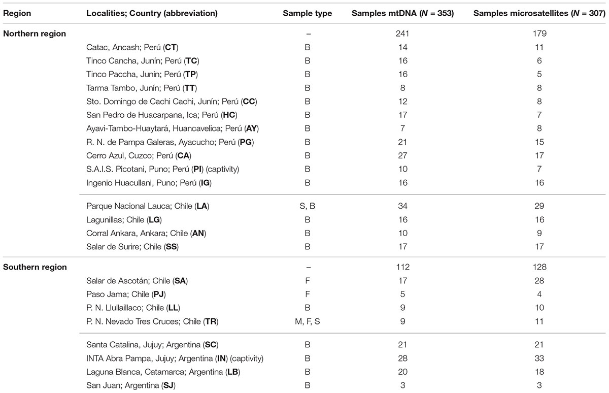
Table 1. Summary of the Vicugna vicugna samples, including localities (ordered north to south), sample type (B, blood; F, fecal; M, muscle; S, skin), number of samples analyzed from each locality for each genetic marker.
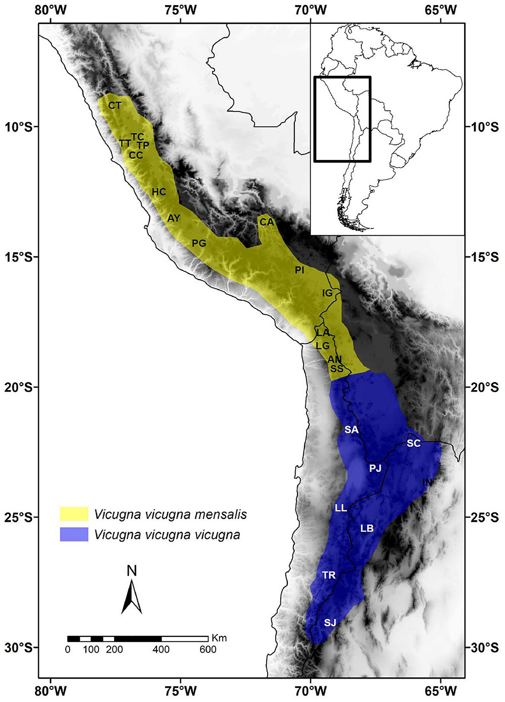
Figure 1. Map of the geographic distribution of Vicugna vicugna mensalis (yellow) and V. v. vicugna (blue) and location of sampled populations in South America. Localities names are: Catac (CT), Tinco Cancha (TC), Tinco Paccha (TP), Tarma Tambo (TT), Sto. Domingo de Cachi Cachi (CC), San Pedro de Hacarpana (HC), Ayavi-Tambo-Huaytará (AY), R. N. Pampa Galeras (PG), Cerro Azul (CA), S.A.I.S. Picotani (PI), Ingenio Hacullani (IG), Parque Nacional Lauca (LA), Lagunillas (LG), Corral Ankara (AN), Salar de Surire (SS), Salar de Ascotán (SA), Paso Jama (PJ), P. N. Llullaillaco (LL), P. N. Nevado Tres Cruces (TR), Santa Catalina (SC), INTA Abra Pampa (IN), Laguna Blanca (LB), San Juan (SJ) (Table 1).
Sample Collection and DNA Extraction
Three hundred and fifty-three samples were collected between 1994 and 2004 at eleven Peruvian and five Chilean localities currently designated as V. v. mensalis; as well as four Argentine and four Chilean localities currently designated as V. v. vicugna (Figure 1 and Table 1). Samples comprised skin (n = 4), muscle (n = 2), blood (n = 333), and feces (n = 37). All samples were stored at -80°C in the Laboratorio de Genómica y Biodiversidad, Departamento de Ciencias Básicas, Facultad de Ciencias, Universidad del Bío-Bío, Chillán, Chile or at CONOPA in Lima, Peru. Total genomic DNA was extracted from blood using the Wizard Genomic DNA Purification Kit (Promega, Madison, WI, United States). DNA from skin and muscle samples was purified using proteinase K digestion and a standard phenol–chloroform protocol (Sambrook et al., 1989). DNA from feces was extracted using the QIAamp DNA Stool Mini Kit (QIAGEN, Valencia, CA, United States) in a separate non-genetic-oriented laboratory.
Mitochondrial DNA
Three hundred and eighty-five base pairs of the left domain of the mitochondrial control region (mtDNA-CR) was amplified using the camelid and vicuña-specific primers LthrArtio (5′- GGT CCT GTA AGC CGA AAA AGG A-3′), H15998V (5′-CCA GCT TCA ATT GAT TTG ACT GCG-3′), Loop007V (5′-GTA CTA AAA GAG AAT TTT ATG TC-3′), H362 (5′-GGT TTC ACG CGG CAT GGT GAT T-3′) (Marín, 2004). Amplification was performed in 50 ml with ∼30 ng genomic DNA, 1x reaction buffer (8 mM Tris-HCl (pH 8.4), 20 mM KCl (Invitrogen, Gibco, Life Technologies, Invitrogen Ltd., Paisley, United Kingdom), 2 mM MgCl2, 25 μM each of dNTP, 0.5 μM each primer and 0.1 U/μl Taq polymerase (Invitrogen, Gibco, Life Technologies). Thermocycling conditions were: 95°C for 10 min, followed by 30–35 cycles of 94°C for 45 s, 62°C for 45 s, 72°C for 45 s, then 72°C for 5 min. PCR products were purified using the GeneClean Turbo for PCR Kit (Bio101) following the manufacturer’s instructions. Products were sequenced in forward and reverse directions using BigDye chemistry on an ABI Prism 3100 semiautomated DNA analyzer, and consensus sequences were generated and aligned using Geneious v.9.1.5 (Biomatters, Auckland, New Zealand). The final alignment was trimmed to 328 bp beginning at the 5′ left domain of the d-loop.
The number of segregating sites (S) and haplotypes (nh), haplotype diversity (h) (Nei, 1987), nucleotide diversity (π) and average number of nucleotide differences between pairs of sequences (k) were estimated using ARLEQUIN 3.5.1.2 (Excoffier and Lischer, 2010). A statistical parsimony network was constructed using TCS v1.21 (Clement et al., 2000) with default settings.
Microsatellite Markers
Fifteen autosomal dinucleotide microsatellite loci (YWLL08, YWLL29, YWLL36, YWLL38, YWLL40, YWLL43, YWLL46 – Lang et al., 1996, LCA5, LCA19, LCA22, LCA23 – Penedo et al., 1998, LCA65, LCA82 – Penedo et al., 1999, and LGU49, LGU68 – Sarno et al., 2000) were analyzed. Amplification was carried out in a 10 μL reaction volume, containing 50–100 ng of template DNA, 1.5–2.0 mM MgCl2, 0.325 μM of each primer, 0.2 mM dNTP, 1X polymerase chain reaction (PCR) buffer (QIAGEN) and 0.4 U Taq polymerase (QIAGEN). All PCR amplifications were performed in a PE9700 (Perkin Elmer Applied Biosystems) thermal cycler with cycling conditions of: initial denaturation at 95°C for 15 min, followed by 40 cycles of 95°C for 30 s, 52–57°C for 90 s and 72°C for 60 s, and a final extension of 72°C for 30 min. Amplification and genotyping of DNA from fecal samples was repeated two or three times. One primer of each pair was labeled with a fluorescent dye on the 5’-end, and fragments analyzed on an ABI-3100 sequencer (Perkin Elmer Applied Biosystems). Data collection, sizing of bands and analyses were carried out using Genemarker v. 1.70 (SoftGenetics).
We identified fecal samples that came from the same individual by searching for matching microsatellite genotypes using the Excel Microsatellite Toolkit (Park, 2001) and eliminated samples from the study if they showed more than 85% overlap. We also evaluated the existence of null alleles using the program Micro-Checker v. 2.2.3 (Van Oosterhout et al., 2004). ARLEQUIN 3.5.1.2 software (Excoffier and Lischer, 2010) was used to estimate allele frequency, observed heterozygosity (HO), and expected heterozygosity (HE). The inbreeding coefficient FIS was estimated following Weir and Cockerham (1984) using FSTAT 2.9.4 (Goudet, 2005).
Genetic Structure and Gene Flow
We used the Bayesian clustering algorithm implemented in STRUCTURE v. 2.3.3 (Pritchard et al., 2000) to group the samples genotyped with microsatellites into K clusters. We tested values of K between 1 and 23, running STRUCTURE five times for each value of K, and using Evanno’s ΔK method to determine the most suitable number of clusters (Evanno et al., 2005). STRUCTURE was run using the admixture model and correlated allele frequencies, as recommended for populations that are likely to be similar due to migration or shared ancestry (Falush et al., 2003; Pritchard et al., 2007). 500,000 iterations were used to estimate K after a burn-in period of 30,000 iterations.
Based on the STRUCTURE results we found K = 2 (Figure 2) to be the most suitable clustering solution (with each cluster corresponding to one subspecies; see results and Figure 2). We used these results to selected the 70 least admixed individuals (35 from northern and 35 from southern localities) to simulate a hybrid population with HybridLab 1.0 (Nielsen et al., 2006). Using these three populations we assessed to which of them each sample in the dataset would be assigned. Furthermore, we also estimated the migration rate between V. v. mensalis and V. v. vicugna and the hybrid population using BayesAss 3.0 (Wilson and Rannala, 2003; Rannala, 2007). We assessed genetic differentiation between sampling localities using FST (Weir and Cockerham, 1984) estimated with the microsatellite data and mitochondrial DNA data in ARLEQUIN 3.5.1.2 (Excoffier and Lischer, 2010) with 10,000 permutations to assess significance. We also estimated pairwise population differentiation between sampling localities with Jost’s D in GENODIVE v.2.0b22 (Meirmans and Van Tienderen, 2004), as this method is independent of the amount of within population diversity (Jost, 2008).
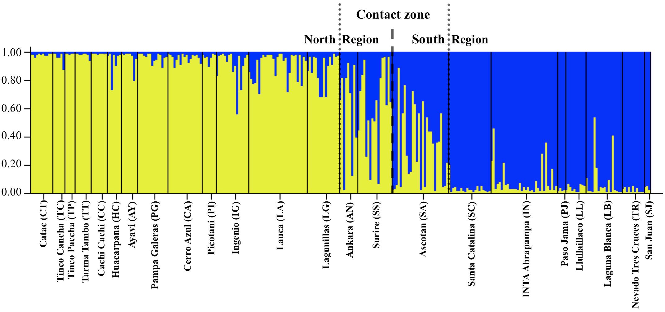
Figure 2. Plot of posterior probability of assignment for 307 vicuñas (vertical lines) to two genetic clusters based on Bayesian analysis of variation at 15 microsatellite loci. Individuals are grouped by locality, and localities are indicated along the horizontal axis. Yellow, Genetic Cluster 1: North group; blue, Genetic Cluster 2: South group.
Spatial Autocorrelation Analyses
We tested for spatial autocorrelation in the data at various distance classes using Genalex 6.5 (Peakall and Smouse, 2012). We used Euclidean genetic and geographic distances between pairs of individuals for the species as a whole and at two additional hierarchical levels: (i) separated for males and females to test for sex-biased dispersal and (ii) separated by subspecies. Correlograms of r-values were estimated as a function of geographic distance using 200-km fixed distance class bins (shorter distances resulted in few observations per bin whereas longer distances compromised resolution of fine-scale genetic structure). We followed Banks and Peakall (2012) to test for correlogram significance and heterogeneity in allele autocorrelation between sex or subspecies groups using Ω and T2 statistics. One thousand bootstrap permutations were used to estimate the 95% confidence intervals around r = 0 (no correlation between genetic variation in individuals in the same bin) and to test if the observed and expected r-values were significantly different form each other. Lastly, we tested for the presence of isolation by distance (IBD) using Mantel tests between the matrix of geographic distances between localities and the matrix of Fst estimated for either the mtDNA or the microsatellite loci.
Migration–Drift Equilibrium
We tested the relative likelihood of a gene flow vs. a genetic drift model using the program 2MOD (Ciofi et al., 1999) (Supplementary Figure 1). Three different datasets were analyzed with 2MOD to test whether the inferred model was affected by the data used. The first dataset consisted of two populations, one made up of the individuals with the highest probability of belonging to V. v. mensalis and the other of the individuals with the highest probability of belonging to V. v. vicugna based on the STRUCTURE results for K = 2 and with a minimum Q threshold of 0.75 indicating the corresponding population ancestry. The second dataset consisted of one population composed of all individuals with a Q-value > 0.5 based on the STRUCTURE results for K = 2 and the other population made up of all the remaining individuals. The third dataset consisted of the data for each locality separately. Each analysis was run independently three times for 200,000 iterations of the Markov Chain Monte Carlo algorithm with the first 10% of the simulations discarded as burn-in.
Demographic History
The mtDNA of the northern and southern regions (one group per subspecies) were used to estimate Tajima’s D and Fu’s Fs statistics (Tajima, 1989; Fu, 1997) with 10,000 simulations to assess significance in ARLEQUIN (Schneider and Excoffier, 1999). These analyses were complemented with Bayesian Skyline Plot (BSP) analyses in BEAST run separately for the individuals of each subspecies (one group per subspecies; Bouckaert et al., 2014). BEAST’s Markov Chain Monte Carlo algorithm was run independently three times for 50 million steps discarding the first 10% as burn-in and until ESS values above 200 would be obtained. A substitution rate of 1.2%/million years was used to scale the BSP in years (as in Almathen et al., 2016).
To identify demographic scenarios that explain current diversity patterns in the northern and southern regions, we used the coalescent-based framework implemented in MSVAR v1.3 (Storz and Beaumont, 2002) using microsatellite loci of each sampling locality (see section “Results”). MSVAR estimates the recent effective population size (N0), the ancestral effective population size (Nt), and the time (t) at which the effective population size changed from Nt to N0. Three independent runs of MSVAR were carried out including wide prior distributions of the model parameters and accounting for the possibility that the populations remained stable over time (Nt ∼ N0), that there was a bottleneck (Nt > N0), or a population expansion (Nt < N0). Prior distributions are log-normal distribution parameterized with the mean and standard deviation for each parameter and truncated at zero following Storz and Beaumont (2002) (Supplementary Table 3). Because there is no vicuña specific microsatellite mutation rate available, we used a range of typical vertebrate microsatellite mutation rates varying between 10-2.5 and 10-4.5 (Weber and Wong, 1993; Di Rienzo et al., 1994; Brohede et al., 2002; Bulut et al., 2009) (Supplementary Table 3). MSVAR was run for a total of 400 million iterations under each demographic model discarding the initial 20% of the MCMC steps as burn-in. The independent runs were used to estimate the mode of the posterior distributions of each parameter (N0, Nt, and t) and their corresponding 90% highest posterior density interval. A generation length of 3 years (Franklin, 1983; González et al., 2006) was used to rescale the t parameter in years. Convergence of the runs was estimated with the Gelman and Rubin’s diagnostic using the CODA library (Plummer et al., 2006) in R (R Development Core Team, 2009).
Results
Genetic Diversity
Among the 353 samples genotyped with microsatellites we detected on average 13 alleles/microsatellite. The number of alleles per locus ranged from 5 to 23, and 38 alleles were unique to a single locality. No deviation from H-W equilibrium was found due to an excess of homozygotes, however, a significant excess of heterozygotes (P < 0.0151, FDR adjusted critical value) was for various markers in different populations, with ten populations showing no deviation from HWE for any locus. The remaining population showed between one and a maximum of eight locus not in HWE, with an overall mean of 2 loci per locality not in HWE. Overall no linkage disequilibrium was found in the sampling localities, with the exception of 12% o the microsatellite pairwise comparisons in Lauca, and one microsatellite pairwise comparison in Lagunillas, another one in Ascotán, and two in Santa Catalina (however, the loci in these comparisons in the last three populations were not the same; FDR adjusted P < 0.00955). Estimates of genetic diversity excluding these loci were not significantly different from those estimated with all loci, thus, we kept these markers for further analyses (Welch corrected t-test -p-value > 0.05). We found consistently moderate to high levels of genetic diversity (mean expected heterozygosity ranged from 0.45 to 0.78) and high values for allelic richness (mean RA ranged from 2.67 to 7.53) (Table 2) relative to other South American mammals, e.g., andean bear (Ruiz-Garcia et al., 2005), guanacos (Marín et al., 2013a), guigna (Napolitano et al., 2015). In the mtDNA we found 52 variable positions (17.33%), 34 transitions, 7 transversions and one insertion among 385 nucleotides, resulting in 57 haplotypes (h = 0.794) among 376 partial sequences of the 5′ end of the control region. Among variable sites, 37 (71.15%) were parsimonious informative. Haplotype (h) and nucleotide diversity (π) ranged between 0–0.92 and 0–0.35 (Table 2). GenBank accession for the publicly available data are AY535173–AY535284 and KY420493–KY420569 for the newly generated sequences.
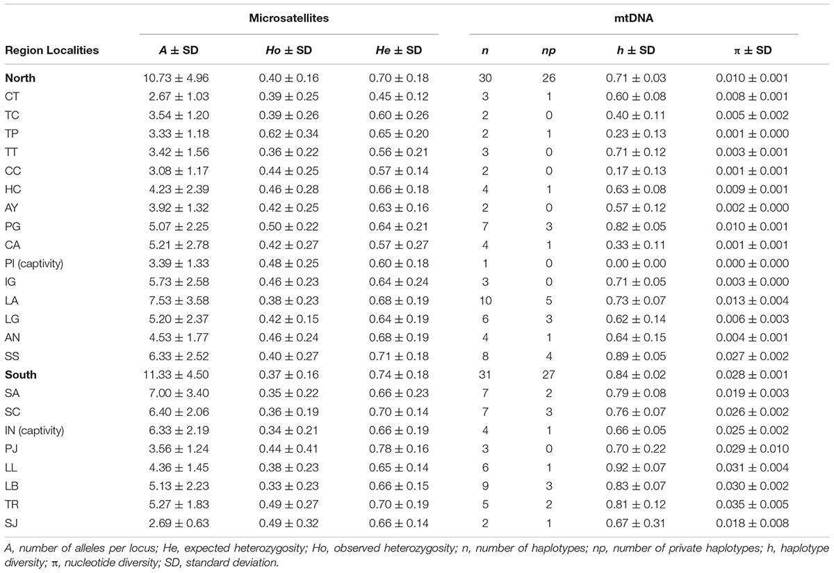
Table 2. Genetic diversity indices from 15 microsatellite loci and mtDNA Control Region sequences by localities (defined in Table 1).
Genetic Structure and Gene Flow
Results of the STRUCTURE analysis indicated that the best clustering solution was K = 2 based on the ΔK method (Supplementary Figures 2A,B) with most of the samples from the Northern region being assigned to one cluster and most of the samples from the Southern region being assigned to the other cluster. Of the 353 individuals, 269 had a clear predominant heritage with Q-values > 0.75. Of the 173 individuals sampled in the Northern region, 155 presented a predominantly northern genetic background, while 20 presented a mixed South – North origin and 4 had clear South genetic heritage with Q-values indicating southern ancestry larger than 0.75 (Table 3). Of the 108 individuals sampled in the Southern Region, 95 presented a predominantly southern genetic background (Q > 0.75), while 13 were of mixed origin, and 2 were assigned to the Northern cluster (i.e., their Q-values indicating a northern ancestry were > 0.75). Overall, most of the individuals of mixed or incongruent heritage in both clusters were sampled in the localities of AN, SS and SA, which correspond to the contact zone between the North and South regions (Figure 2 and Table 3).
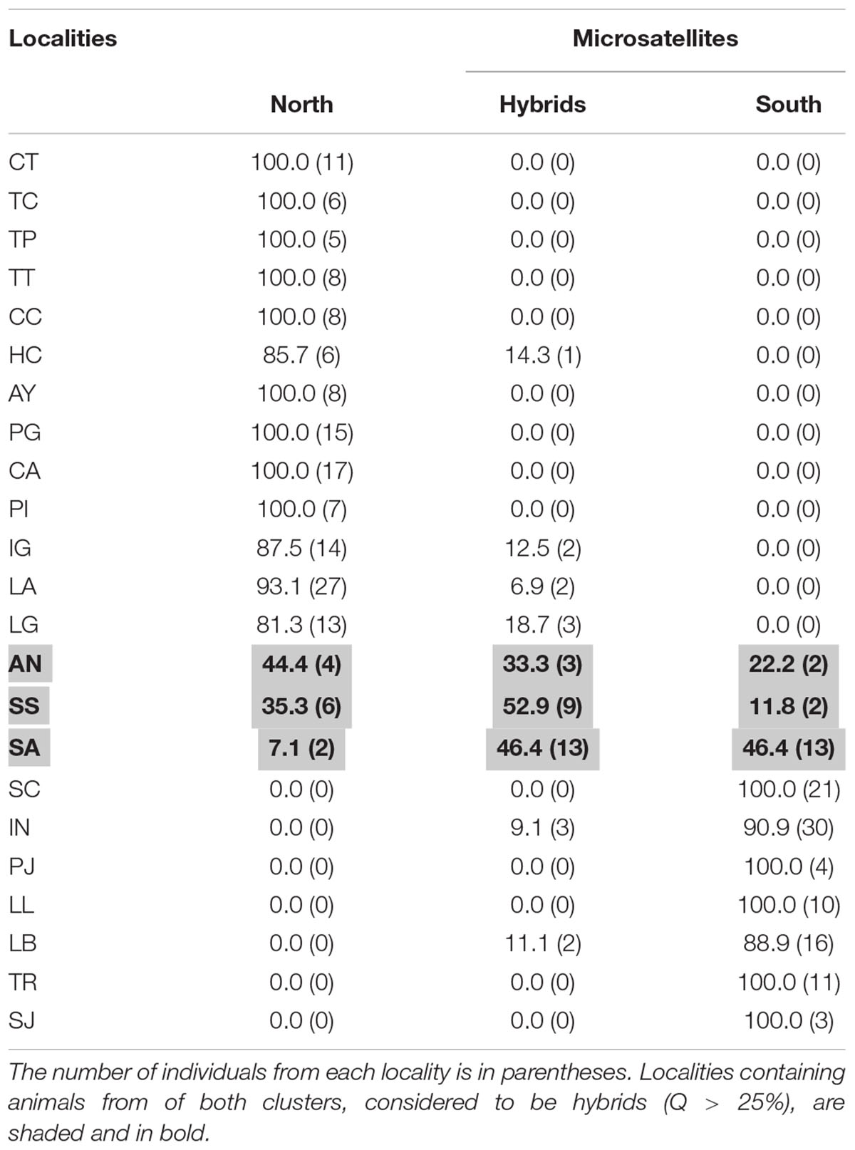
Table 3. Percentage of individuals assigned to the North or South genetic clusters with nuclear DNA (Q > 75%, STRUCTURE analysis).
The pairwise analysis of divergence between sampling localities showed significant genetic differentiation between ∼58% of the localities pairwise comparisons measured with the FST and (D)phi-st (Supplementary Table 1). Significant pairwise differentiation estimated with FST ranged from low (0.037) to high values (0.612), with the greatest divergence observed between the CC and PI localities. D pairwise divergence values were larger than the FST values with significant values ranging between 0.19 and 0.95 and the highest divergence observed between the AY and PI localities. Furthermore, we also found a significant negative correlation (-0.56; P ∼2.2e-16) in average heterozygosity and pairwise FST between sampling localities suggesting that the observed divergence between localities may be driven by genetic drift rather than the build up of unique mutations present at the different localities (Weeks et al., 2016).
When dividing the samples into two groups representing the two clusters identified by STRUCTURE reflecting the two subspecies, the FST including and excluding hybrids were 0.0779 and 0.0998, respectively, and both were significant (p < 0.005). A division between the North and South regions was also observed with the haplotype network calculated with the 57 mtDNA Control Region haplotypes (Figure 3). Among these haplotypes 28 were found in V. v. mensalis (North) and 25 were found only in V. v. vicugna (South), while four where shared between the two subspecies and thus found in both the North and South Regions (haplotype 2, 6, 17, and 21). Additionally, haplotypes 27, 29, and 30 found only on V. v. mensalis grouped together with those of V. v. vicugna, while haplotypes 33 and 34 found only on V. v. vicugna clustered with to the V. v. mensalis haplotypes. The 57 haplotypes are connected with a maximum of 48 mutational steps, with most genetic variation localized regionally and the main link between the two geographic regions of the network diverging by five mutations. Consistent with the STRUCTURE results, the haplotypes shared between the two regions occurred in the sampling localities in the contact zone (AN, SS, and SA).
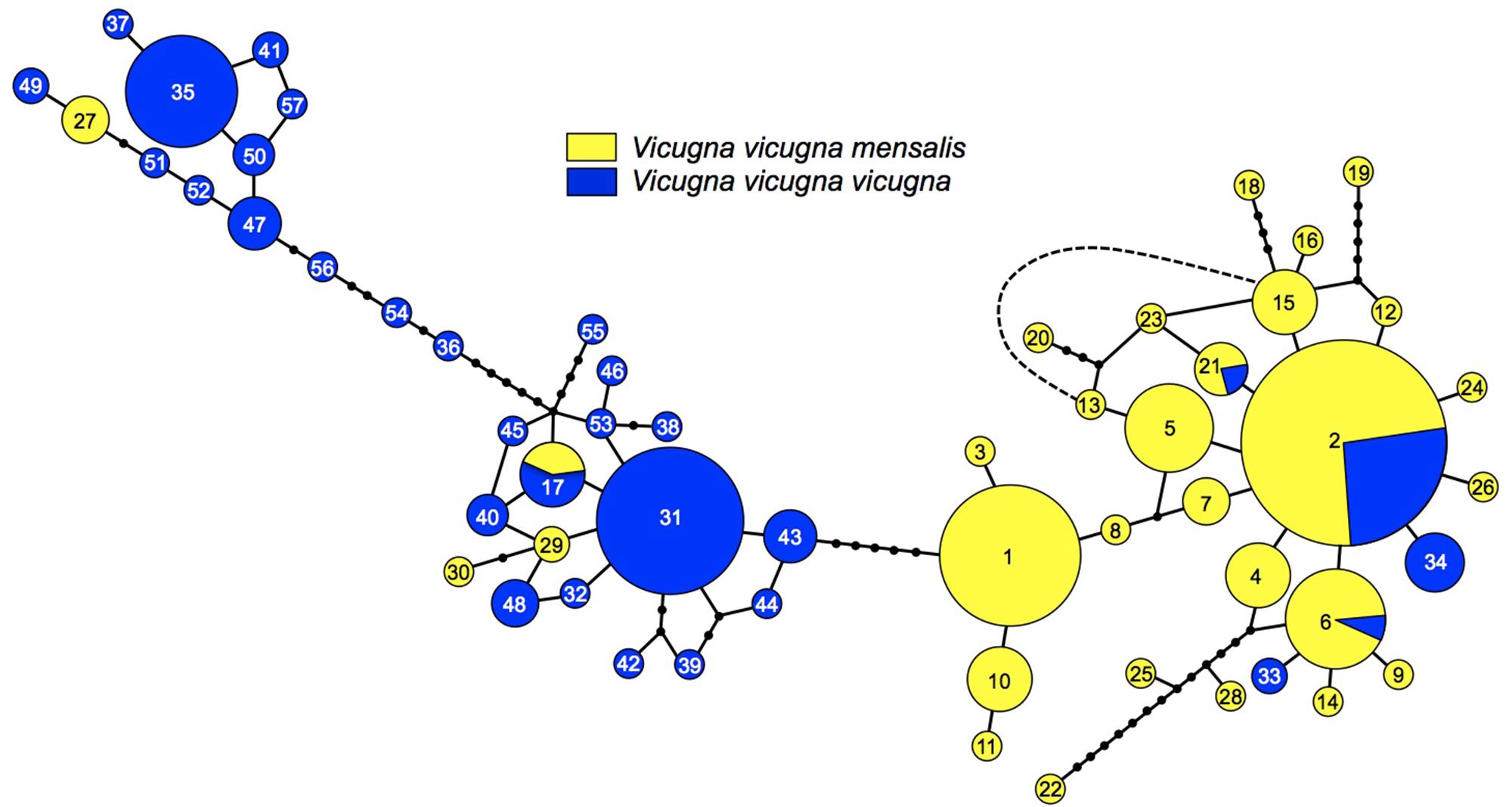
Figure 3. Minimum spanning network representing the relationships among 57 control region haplotypes, numbers represent each haplotype (see Supplementary Table 2). Circle sizes correspond to haplotype frequencies. Branches without circles correspond to one difference between haplotypes, and each small black circle corresponds to one additional mutation. Dashed line represents one mutational step between haplotypes 13 and 16.
Spatial Autocorrelation Analysis
We found significant spatial autocorrelation among individuals for the species as whole (Ω = 96.9 = 7, p < 0.001) and at both hierarchical levels, implying dispersal is limited at the spatial scale, with greater resemblance between individuals at shorter distances and decreasing resemblance as distance increases. Although both males and females presented a spatial autocorrelation pattern indicative of isolation by distance, these were significantly different from each other (Ω = 62.3, p < 0.001) with females presenting almost twice as much similarity than males at the smaller distance class (T2 = 63.5, p < 0.001 – 200 km distance class). None the less, as geographical distance increases the differences between r-values in both sexes almost disappears (Figures 4A,B). We also found significant differences in autocorrelation between subspecies (Ω = 36.2, p < 0.001; Figures 4C,D) with the northern vicuña showing a stronger effect of geographic distance on their similarity than in the southern vicuña which shows approximately the same similarity across all distance classes. The analysis of IBD using Mantel tests with the mtDNA data resulted in a significant correlation between the matrix of geographic distances between localities and the Fst between localities (r ∼ 0.36, p-value = 0.00016). Equivalent results were obtained for this analysis using the microsatellite data (r ∼ 0.38, p-value = 0.00001).
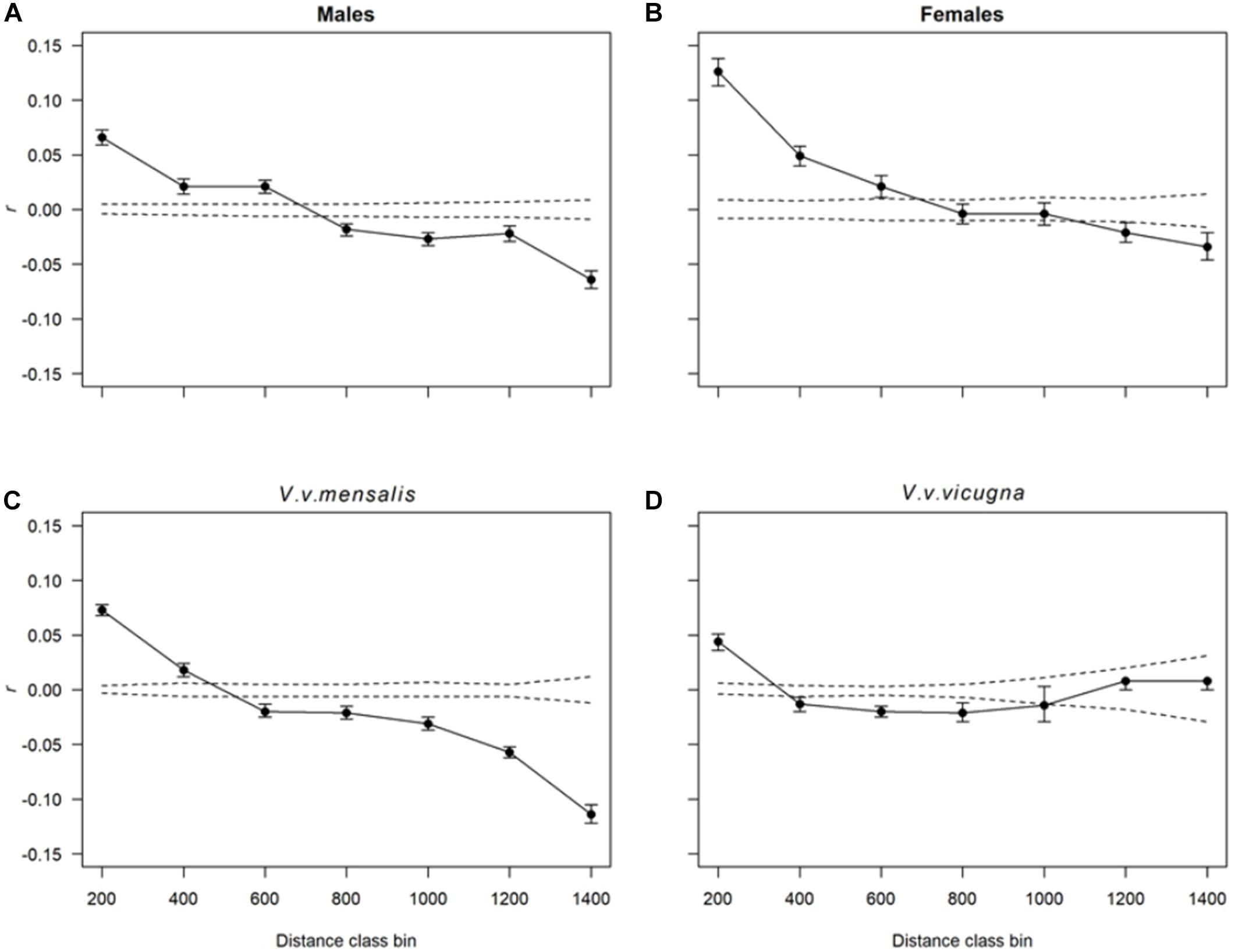
Figure 4. Correlograms showing the combined spatial correlation r across transects as a function of distance. Dotted lines correspond to the 95% CI about the null hypothesis of a random distribution of genetic variation over space (i.e., no effect of geographic distance on r). Each r value has 95% confidence error bars shown. Distance class bins are shown in kilometers. Each plot shows the autocorrelation for distance class sizes of 200 km estimated for (A) males, (B) females, (C) all northern vicuñas (V. v. mensalis) and (D) southern vicuñas (V. v. vicugna).
Migration–Drift Equilibrium
Results of the coalescent analyses to tests for gene flow + genetic drift vs. a genetic drift only model showed that all simulations support a genetic drift + gene flow model as an explanation of the observed genetic variability (the posterior probability of the model of genetic drift + gene flow was higher than 0.98 for all tests; Supplementary Table 5). This result is the same for all three alternative dataset configurations tested and indicates that vicuña localities have historically not been isolated from each other but, rather, inter connected.
Demographic History
Based on the mtDNA data, the North Region showed negative Fu’s F-values (Fs = -2.3279, P < 0.05) and Tajima’s D (D = -1.7341, P > 0.05) consistent with a pattern of population expansion, however, Tajima’s D was not significant. For the South region both tests were not significant (Fs = -0.0863, P > 0.10; D = 1.2433, P > 0.05) suggesting a stable population history. These results are consistent with the presence of a major haplotype in the northern region (Hap2), while in the southern region two distantly related haplotypes occur at moderate to high frequency (Hap31 and 35) with many low frequency haplotypes in between them. The BSP analysis for each subspecies clearly shows a higher effective population size for V. v. mensalis (Figures 5A,B). This same analysis also supports a recent population expansion for both V. v. mensalis and V. v. vicugna starting approximately 3,000 years ago (Figures 5A,B). However, V. v. mensalis presents a population decrease starting approximately 800 years ago (Figure 5A).
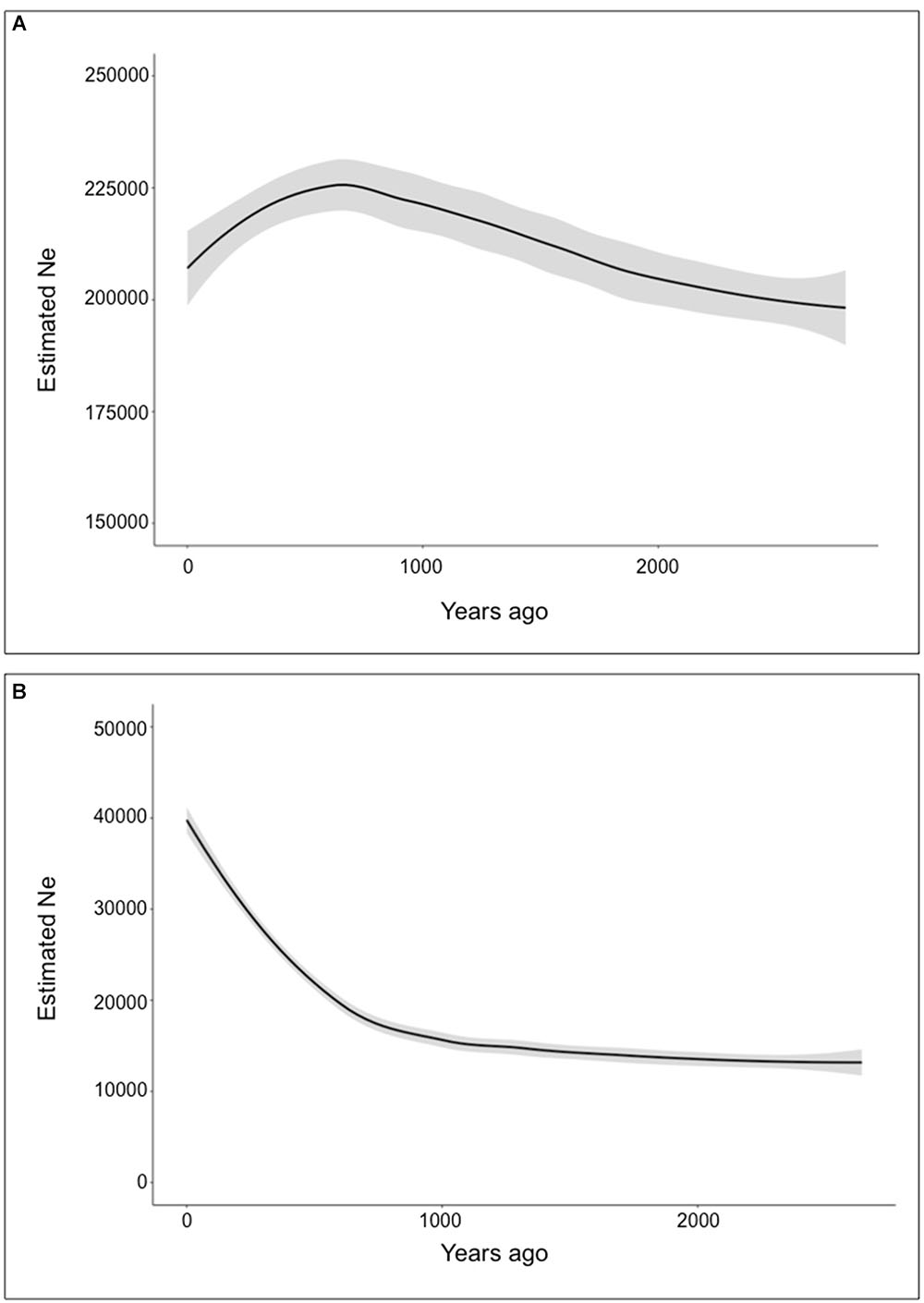
Figure 5. Demographic analysis of Vicugna vicugna using the Bayesian Skyline Plot Method. Gray background represents error margins. (A) Bayesian Skyline Plot of Vicugna vicugna mensalis. (B) Bayesian Skyline Plot of Vicugna vicugna vicugna.
The demographic analysis using the microsatellite data and MsVar showed consistent results under all three demographic models tested, i.e., (1) no demographic change, (2) bottleneck and (3) population expansion. The three independent runs for each sampling locality presented Gelman and Rubin’s statistics lower than 1.2. In all cases MSVAR detected evidence for major effective population size decline at all localities, consistent with current or recent small census sizes (Figure 6 and Supplementary Table 3). All localities analyzed presented large ancestral effective population sizes on the order of ∼22,000 individuals [with 95% highest posterior density intervals (HPD) between ∼5,000 and ∼100,000; Supplementary Table 3]. Across localities the time of the bottleneck was on average ∼7,600 years before the present (YBP; HPD ∼760–125,000 YBP). Following this event, the effective population size in vicuña reached on average less than 1,000 (HPD ∼200–∼22,000; Supplementary Table 4). Similar ancestral effective population size and bottleneck dates, combined with the results of migration–drift and isolation by distance analyses, suggests that current vicuñas descend from a single large ancestral population that only recently started diverging probably through genetic drift.
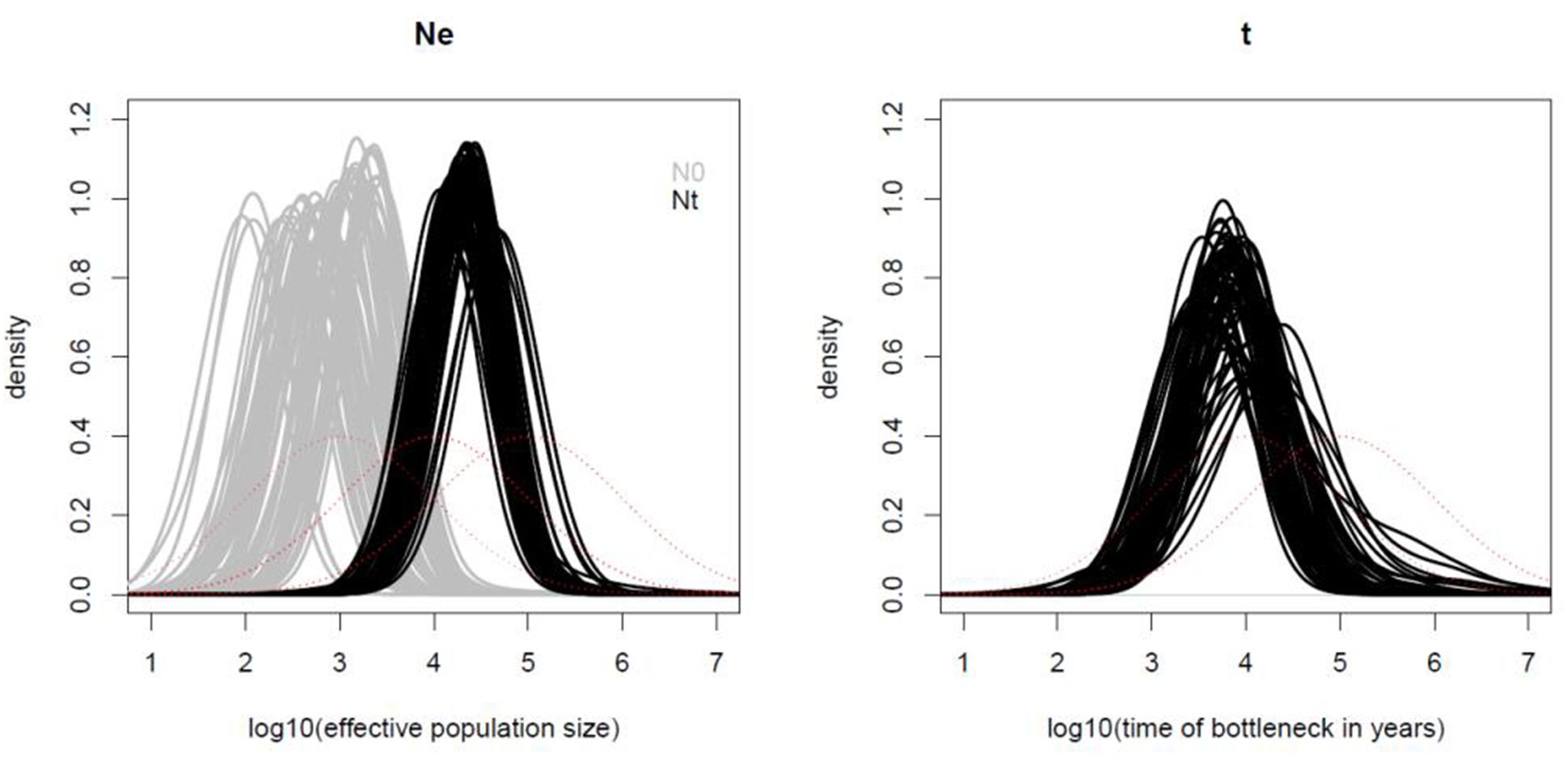
Figure 6. Demographic analysis of Vicugna vicugna with MsVar. Panel (A) shows the posterior distributions of the current effective population size (gray lines), and ancestral effective population size (black lines). The time of the bottleneck (black lines) is shown in panel (B) for each of the three MSVAR replicates for each locality analyzed. The x-axis values are in log scale (e.g., 2 means 102). The red lines show the prior distributions.
Discussion
Here, we present the most comprehensive analysis to date of genetic variation in vicuña across the species range. The molecular markers used present contrasting patterns regarding vicuña evolutionary history with conflicting evidence regarding the split of the species into two different taxonomic units. For instance, analysis of the mtDNA haplotypes largely supports a split into two vicuña groups, with each group dominated by haplotypes specific to the northern (i.e., V. v. mensalis) or the southern (i.e., V. v. vicugna) groups, respectively. This apparent differentiation is supported by the divergence analysis that results in a large and significant ΦCT of 0.4. Nevertheless, some haplotypes are shared between the two groups of vicuñas, particularly at localities in the contact zone between 18°S (Ankara, AN) and 21°S (Salar de Ascotan, SA). The data presented here evidences gene flow between the two vicuña types as reflected by haplotype sharing between animals of each type (e.g., haplotypes 2, 6, 17, and 21) deriving from localities at or near the contact zone between the two types (Salar de Ascotan, Santa Catalina, Lauca, Salar de Surire). This is further supported the observation of phenotypically mensalis individuals that carry vicugna haplotypes (i.e., seven individuals from Salar de Surire carrying haplotypes 27 (four animals), 29 (2 animals), and 30 (1 animal) and conversely, phenotypically vicugna individuals that carry mensalis haplotypes (i.e., two individuals from Salar de Ascotan carrying haplotype 33 and one carrying haplotype 34, and four individuals from Santa Catalina carrying haplotype 33).
STRUCTURE analysis of the microsatellite data also identifies the presence of two clusters in the dataset (K = 2), and supports a contact zone between the two clusters where animals in that region present composite genotypes at intermediate allele frequencies to those observed in more northern or southern vicuñas (Figure 2). Our dataset did not include animals from Bolivia, a region in the contact zone between the two clusters identified here. However, we expect that considering Bolivia’s location, vicuña samples from that part of the range might belong to the hybrid set of genotypes detected here for the contact zone. Such a pattern would explain the lack of taxonomic differentiation previously observed in Bolivia (Sarno et al., 2004). Interestingly, the contact zone between the two vicuña distribution ranges broadly coincides with the area occupied by the Tauka palaeolake which formed after the last glacial maximum and disappeared around 8,500 years ago (Blard et al., 2011). At its maximum, 16,000–14,500 BP, Tauka palaeolake is thought to have covered more than 52,000 km2 (i.e., ∼75% the size of Lake Victoria in Africa) including the extant Lake Poopó and the Coipasa and Uyuni saltpans. However, following its disappearance, a narrow area between the mountains to the east of the Atacama Desert and the Uyuni saltpan opened enabling contact between the two vicuña groups, which otherwise would have been separated by the presence of this large lake in the Andean altiplano.
The best clustering solution identified by STRUCTURE with the microsatellite data, while reminiscent of the mtDNA split between the two vicuña subspecies, is more likely the outcome of isolation by distance (see Mantel test results and spatial autocorrelation) where individuals from localities at one end of the range distribution are more likely to resemble each other than individuals on the opposite end of the range. In such a scenario, instead of two populations being present, the data represents a single population with a gradient of intermediate genotypes between two contrasting extremes, as observed in Figure 2. Consistent with such pattern, individuals from the localities in the contact zone between the North and South ranges (i.e., Ankara, Surire and Ascotan), present a variety of genotypes ranging from mostly belonging to one of the two groups to almost presenting 50% ancestry from each group, while animals beyond this region are mostly of one genetic background. This is further supported by the phylogeographic analysis of the DBY gene of the Y chromosome which found no evidence for differences between V. v. mensalis y V. v. vicugna (Marín et al., 2017).
The change in genetic similarity between animals at increased distance was also observed with the spatial autocorrelation analyses. While splitting the dataset by sex resulted in both groups showing approximately the same isolation by distance pattern, females were more similar to each other at smaller distances (e.g., 200–400 km) than males. This pattern is consistent with females behaving more philopatric than males, with the later leaving their family groups upon becoming yearlings and form non-territorial bachelor groups which frequently have to move because of conflicts with local males with established territories (Koford, 1957; Franklin, 1983; Arzamendia et al., 2018). Yet, both females and males contributed similarly to gene flow at distance classes from 600 to 800 km, suggesting that beyond 800 km the effect of gene flow is limited, as few animals (if any) move that far.
A different pattern of spatial autocorrelation was observed when separately analyzing the northern and southern vicuñas. While northern vicuñas show the same isolation by distance pattern discussed above (Figure 4), the autocorrelogram for the southern vicuña drops quickly between 200 and 400 km, then seems to level off with similar r-values across further distances. Northern vicuñas inhabit a geographic range with higher habitat productivity and wider dietary resource availability than southern vicuñas. Thus, while northern vicuñas can find food resources in relative proximity (Franklin, 1982), southern vicuñas need to move over longer distances to find them, thereby increasing the probability of reproduction with animals that otherwise would be too far away (Arzamendia et al., 2018). However, such difference can also be achieved by populations with different levels of genetic variation, where populations with lower genetic diversity will experience a stronger effect of geographic distance if gene flow is low (as in northern vicuñas), while populations with a higher genetic diversity (as in southern vicuñas) need of a stronger reduction in gene flow to result in the same spatial pattern.
Extant vicuña populations are assigned to one of the two recognized vicuña subspecies; however, while these may present some morphological differences possibly reflecting local adaptation, their genetic variation suggests they form two extremes of a genetic continuum. Further evidence about the joint evolution of the two vicuña groups is provided by demographic modeling of the history of the various localities analyzed here, and assessment of whether these localities evolved independently from each other or connected via gene flow. The demographic analysis with MSVAR found that the extant vicuña genetic variation is the outcome of strong bottleneck that occurred ∼7,600 YBP (HPD ∼760–125,000 YBP). However, what is remarkable, is not only that all extant populations seem to have passed through this bottleneck at approximately same time, they all had a very similar ancestral effective population size (i.e., ∼25,000–HPD ∼5,000–100,000). It is likely that a single large vicuña population occupied a wide range across the Andes prior to a relatively recent bottleneck that dramatically reduced the effective population size to less than 1,000 (HPD ∼50–10,000). The main consequence of this event was fragmentation and isolation of previously well connected vicuña populations within their present distribution area (9°S to 29° S) and the small effective population size of pocket populations that survived. This hypothesis is supported by comparison of the model of evolution under genetic drift against a model that also included gene flow and which unambiguously showed that the latter better explains the extant genetic variation. While this analysis does not indicate modern connectivity between these localities, as has been previously suggested for vicuña (Casey et al., 2018), it supports that connection between them has been a major factor in the recent evolutionary history of V. vicugna.
The average bottleneck estimate across the vicuña populations is ∼7,600 YBP, but the range of variation from ∼700–125,000 YBP (Supplementary Table 4) reflect the uncertainty associated with estimates like generation length and mutation rate. Thus, while it is tempting to try to associate the inferred bottleneck with a particular event during the South American Holocene, it is safer to assume that it occurred sometime over the last 12,000 years. This period has been marked by dramatic changes across South America including the establishment of human hunters in the Peruvian high Andes ∼9,000 YBP (Aldenderfer, 1999) who, by ∼6,000 YBP, specialized on vicuña and guanaco (Wheeler et al., 1976). Additionally, this period of time included the transition from hunting to herding, with domestication of vicuña ∼6,000–5,500 YBP (Wheeler, 1995). It is possible that any or all of these events contributed to the demographic signal observed here, however, we are not able to pinpoint a single event. While the consistent results obtained across vicuña populations are indicative of the robustness of the genetic signature of the demographic change (Chikhi et al., 2010; Peter et al., 2010), future studies should be carried out using larger datasets (e.g., genome-wide polymorphisms) and other methodologies that are likely to result in narrower confidence intervals of parameters of interest (e.g., approximate Bayesian computation).
Conservation Implications
Management Units
The evolutionary history of extant vicuñas is not at odds with the observation of morphological differences between animals across its range. In fact, it indicates that despite environmental changes during the Late Pleistocene and Holocene, V. vicugna maintained its genetic and taxonomic identity through time. Moreover, this identity remained despite the human population expansion in South America (<12,000 YBP) and their specialization in hunting vicuña (and guanaco) (Wheeler et al., 1976), as well as domestication of the vicuña at 6,000–5,500 YBP (Baid and Wheeler, 1993; Wheeler, 1995, 2012). Morphological variation across vicuña is likely to reflect the extensive territory they occupy and the different ecologies they are exposed to. Hence, morphological differences between the northern and southern groups would conform to ecotypes, as in other species, even if those where differences are not obviously reflected by the molecular markers used here (Courtois et al., 2003).
Establishing MUs is difficult because of differentiation by distance and the influence of genetics pools at sampled localities. MU determination depends on geographic areas with independent demographic dynamics between populations, whose individuals present a well-defined genetic structure and low migration rates (Marín et al., 2013a; Sveegaard et al., 2015; Yannic et al., 2016). At the large continental scale, it was not possible for us to identify discrete genetic clusters differentiating localities along the vicuña distribution range in this study, as it was in the study of Peruvian vicuña populations (Wheeler et al., 2001); therefore we propose the use of “continuous” MUs for the species. The main reason for this is that vicuña populations are defined by distance instead of by population discrete fragmentation or geographical barriers. By implementing this approach it is possible to include the spatial correlation information in defining the management area dimensions (e.g., 0–200 km) and protective actions for each locality (e.g., Caughley, 1994), which would enable extending the proposed MUs of Wheeler beyond the only four groups identified in their work (Wheeler et al., 2001).
Captive Populations
Two captive populations were included in this study Abra Pampa (Argentina) and Picotani (Peru). These populations present lower genetic variation as measured with both types of molecular markers than their immediate wild neighboring populations (i.e., Santa Catalina and Ingenio, respectively). The Abra Pampa Experimental Station has had captive vicuñas since 1933 (see Mosa, 1987). Although today’s captive population is ∼1,200 individuals (Boswall, 1972; Mosa, 1987; Canedi and Pasini, 1996; Vicuña Convention, 2017) it has been reported that the founding population may have been as few as 22 animals (Canedi and Pasini, 1996). Our results suggest that this population has lower allelic richness and haplotypic diversity indexes than the other localities, probably as a consequence of a founder effect. None the less, the Abra Pampa confinement system has not resulted in a substantial loss of heterozygosity, supporting the hypothesis that a constant but low flow of wild vicuña into the captive herd has taken place (Anello et al., 2016). On the other hand, the Picotani animals have been in captivity since 1997 and they are completely enclosed and there is no breeding with wild vicuña. Our results indicate that the majority of genetic diversity estimators show a reduction in genetic variation in this captive population (e.g., only one mtDNA haplotype was found in comparison to three in neighboring Ingenio) probably due to the founder effect and despite of the larger starting population relative to Abra Pampa. The poor mtDNA genetic variation in captive animals from Picotani is worrying if some management decisions are taken at short-term such as releasing into the wild or translocating for repopulation or productive purposes, therefore a genetic impact assessment is urgently needed for decision support. These results help both setting a basal line for monitoring genetic diversity in these captive populations, but also provide information relevant for the development of an improved long-term captive management strategy at both locations to mitigate the observed loss of genetic variation.
Conclusion
Here, we present the most extensive genetic analysis of Vicugna vicugna to date. These results suggest that the two morphological variants of vicuña, i.e., the northern V. v. mensalis and the southern V. v. vicugna, were until recently closely interconnected with each other, or probably part of a single large population that passed through a strong bottleneck that left small isolated populations across a vast geographic range. Furthermore, extant vicuña genetic variation is better explained by a model of isolation by distance rather than by two discrete populations. However, given the extent of the vicuña geographic range and variation in the environments therein, it is likely that vicuña populations differ to some extent due to adaptation to local environmental variables. We propose the use of continuous MU for vicuña conservation and that this data serve as a baseline for genetic variation monitoring to avoid further loss of genetic diversity in captivity.
Ethics Statement
Samples were collected following guidelines of the American Society of Mammalogists (Sikes et al., 2011). Specific permits were required for the Servicio Agrícola y Ganadero, SAG (permit 447, 2002), the Corporación Nacional Forestal, CONAF (permit 6/02, 2002), for granting other collection permits and helping in collecting samples. The animal research oversight committee of Universidad del Bío-Bío had knowledge of sampling plans prior to their approval of the present animal research protocol. All experimental protocols were approved by the Institutional Animal Care and Use Committee of Universidad del Bío-Bío, the methods were carried out in accordance with the approved guidelines.
Author Contributions
JM developed the ideas and obtained funding for the project. JW, BG, and JM collected the samples. JV, JC, RR, NA, and AC conducted the DNA analyses. AC, AA, DG-U, VV, and PO-tW analyzed the data. JM, BG, DG-U, JW, and PO-tW wrote the manuscript. All authors read, commented on and approved the final manuscript.
Funding
In Chile this research was supported by FONDECYT grant 1140785, CONICYT (Beca de Apoyo a Tesis Doctoral and Redes Internacionales para Investigadores en Etapa Inicial REDI170208). DG-U receives funding through Núcleo Milenio INVASAL from Iniciativa Científica Milenio, sponsored by Chile’s Ministerio de Economía, Fomento y Turismo. In Peru, research was supported by Darwin Initiative for the Survival of Species (United Kingdom) grant 162/06/126 (1997–2000), The British Embassy (Lima), NERC (United Kingdom) grant GST/02/828 (1994–1998), the European Commission INCO-DC ICA4-2000-10229, MACS (2001–2005), and a Newton Fund Researcher Links Travel grant (ID: RLTG9-LATAM-359537872) funded by the United Kingdom Department for Business, Energy and Industrial Strategy and CONCYTEC (Peru) and delivered by the British Council; Asociación Ancash, Peru (2004); FINCyT Perú grant 006-FINCyT-PIBAP-2007 (2008–2010); and COLP, Compañía Operadora de LNG del Perú contract PLNG-EV-09012 (2010–2011).
Conflict of Interest Statement
The authors declare that the research was conducted in the absence of any commercial or financial relationships that could be construed as a potential conflict of interest.
Acknowledgments
In Chile, we thank the Servicio Agrícola y Ganadero, SAG, the Corporación Nacional Forestal, CONAF for granting other collection permits and help in collecting samples Cristian Bonacic (Pontificia Universidad Católica de Chile), Pablo Valdecantos (Universidad Nacional de Tucumán), Bibiana Vilá (Universidad de Lujan), Luis Jacome (Zoológico de Buenos Aires, Argentina) and Alberto Duarte (Zoológico de Mendoza, Argentina) for sharing samples. Samples were collected under permits from CONACS, SERNANP and DGFFS (details above). Special thanks go to Carlos Loret de Mola and Maria Luisa del Rio (CONAM), Domingo Hoces, Wilder Trejo, Daniel Rivera, Daniel Arestegui, Leonidas Rodriguez, and Dirky Arias (CONACS); Gustavo Suarez de Freitas and Antonio Morizaki (INRENA); Felipe San Martin (Facultad de Medicina Veterinaria, Universidad Nacional Mayor de San Marcos) and Alejandro Camino (Asociacion Ancash). Over the years, David Perez, Antony Rodriguez, Juan Manuel Aguilar, and Paloma Krüger have helped in collecting samples. At CONOPA, Domingo Hoces, Lenin Maturrano, Alvaro Veliz, Katherine Yaya, Juan Olazabal, Raul Rosadio, and Michael Bruford have all contributed to the research reported here – from sampling to laboratory analysis and interpretation of the results.
Supplementary Material
The Supplementary Material for this article can be found online at: https://www.frontiersin.org/articles/10.3389/fgene.2019.00445/full#supplementary-material
References
Acebes, P., Wheeler, J., Baldo, J., Tuppia, P., Lichtenstein, G., Hoces, D., et al. (2018). Vicugna vicugna. The IUCN Red List of Threatened Species 2018: e.T22956A18540534. Available at: https://www.iucnredlist.org/species/22956/18540534 (accessed May 4, 2019).
Aldenderfer, M. (1999). The Pleistocene/Holocene transition in Peru and its effects upon human use of the landscape. Quat. Int. 53/54, 11–19. doi: 10.1016/s1040-6182(98)00004-4
Almathen, F., Charruau, P., Mohandesan, E., Mwacharo, J. M., Orozco-terWengel, P., Pitt, D., et al. (2016). Ancient and modern DNA reveal dynamics of domestication and cross-continental dispersal of the dromedary. Proc. Natl. Acad. Sci. U.S.A. 113, 6707–6712. doi: 10.1073/pnas.1519508113
Ammann, C., Jenny, B., Kammer, K., and Messerl, I. B. (2001). Late quaternary glacier response to humidity changes in the arid Andes of Chile (18–29° S). Palaeogeogr. Palaeoclimatol. Palaeoecol. 172, 313–326. doi: 10.1016/s0031-0182(01)00306-6
Anello, M., Daverio, M. S., Romero, S. R., Rigalt, F., Silbestro, M. B., and Vidal-Rioja, L. (2016). Genetic diversity and conservation status of managed vicuña (Vicugna vicugna) populations in Argentina. Genetica 144, 85–97. doi: 10.1007/s10709-015-9880-z
Arzamendia, Y., Carbajo, A. E., and Vilá, B. (2018). Social group dynamics and composition of managed wild vicuñas (Vicugna vicugna vicugna) in Jujuy, Argentina. J. Ethol. 36, 125–134. doi: 10.1007/s10164-018-0542-3
Baid, C. A., and Wheeler, J. (1993). Evolution of high Andean Puna ecosystems: environment, climate, and culture change over the last 12,000 years in the central Andes. Mt. Res. Dev. 13, 145–156.
Baigún, R. J., Bolkovic, M. L., Aued, M. B., Li Puma, M., and Scandalo, R. (2008). Manejo de Fauna Silvestre en la Argentina. Primer Censo Nacional de Camélidos Silvestres al Norte del Río Colorado. Buenos Aires: Secretaría de Ambiente y Desarrollo Sustentable de la Nación.
Banks, S. C., and Peakall, R. O. D. (2012). Genetic spatial autocorrelation can readily detect sex-biased dispersal. Mol. Ecol. 21, 2092–2105. doi: 10.1111/j.1365-294X.2012.05485.x
Blard, P. H., Sylvestre, F., Tripati, A. K., Claude, C., Causse, C., Coudrain, A., et al. (2011). Lake highstands on the Altiplano (Tropical Andes) contemporaneous with Heinrich 1 and the Younger Dryas: new insights from 14C, U–Th dating and δ18O of carbonates. Quat. Sci. Rev. 30, 3973–3989. doi: 10.1016/j.quascirev.2011.11.001
Bouckaert, R., Heled, J., Kühnert, D., Vaughan, T., Wu, C.-H., Xie, D., et al. (2014). BEAST 2: a software platform for bayesian evolutionary analysis. PLoS Comput. Biol. 10:e1003537. doi: 10.1371/journal.pcbi.1003537
Brohede, J., Primmer, C. R., Moller, A., and Ellegren, H. (2002). Heterogeneity in the rate and pattern of germline mutation at individual microsatellite loci. Nucleic Acids Res. 30, 1997–2003. doi: 10.1093/nar/30.9.1997
Bulut, Z., McCormick, C. R., Gopurenko, D., Williams, R. N., Bos, D. H., and DeWoody, J. A. (2009). Microsatellite mutation rates in the eastern tiger salamander (Ambystoma tigrinum tigrinum) differ 10-fold across loci. Genetica 136, 501–504. doi: 10.1007/s10709-008-9341-z
Canedi, A. A., and Pasini, P. S. (1996). Repoblamiento y bioecologia de la vicuna silvestre en la Provincia de Jujuy, Argentina. Anim. Genet. Resour. 18, 7–21. doi: 10.1017/s1014233900000663
Casey, C. S., Orozco-terWengel, P., Yaya, K., Kadwell, M., Fernández, M., and Marín, J. C. (2018). Comparing genetic diversity and demographic history in codistributed wild South American camelids. Heredity 121, 387–400. doi: 10.1038/s41437-018-0120-z
Chikhi, L., Sousa, V. C., Luisi, P., Goossens, B., and Beaumont, M. A. (2010). The confounding effects of population structure, genetic diversity and the sampling scheme on the detection and quantification of population size changes. Genetics 186, 983–995. doi: 10.1534/genetics.110.118661
Ciofi, C., Beaumontf, M. A., Swingland, I. R., and Bruford, M. W. (1999). Genetic divergence and units for conservation in the Komodo dragon Varanus komodoensis. Proc. R. Soc. Lond. B Biol. Sci. 266, 2269–2274. doi: 10.1098/rspb.1999.0918
Clement, M., Posada, D., and Crandall, K. A. (2000). TCS: a computer program to estimate gene genealogies. Mol. Ecol. 9, 1657–1659. doi: 10.1046/j.1365-294x.2000.01020.x
Courtois, R., Bernatchez, L., Ouellet, J.-P., and Breton, L. (2003). Significance of caribou (Rangifer tarandus) ecotypes from a moleculargenetics viewpoint. Conserv. Genet. 4, 393–404. doi: 10.1023/A:1024033500799
Di Rienzo, A., Peterson, A. C., Garza, J. C., Valdes, A. M., Slatikin, M., and Frimer, N. B. (1994). Mutational processes of simple-sequence repeat loci in human populations. Proc. Natl. Acad. Sci. U.S.A. 91, 3166–3170. doi: 10.1073/pnas.91.8.3166
Escalante, M. A., García-De-León, F. J., Dillman, C. B., de los Santos Camarillo, A., George, A., and Barriga-Sosa, I. D. L. A. (2014). Genetic introgression of cultured rainbow trout in the Mexican native trout complex. Conserv. Genet. 15, 1063–1071. doi: 10.1007/s10592-014-0599-7
Evanno, G., Regnaut, S., and Goudet, J. (2005). Detecting the number of clusters of individuals using the software STRUCTURE: a simulation study. Mol. Ecol. 14, 2611–2620. doi: 10.1111/j.1365-294x.2005.02553.x
Excoffier, L., and Lischer, H. E. L. (2010). Arlequin suite ver3.5: a new series of programs to perform population genetics analyses under Linux and Windows. Mol. Ecol. Resour. 10, 564–567. doi: 10.1111/j.1755-0998.2010.02847.x
Falush, D., Stephens, M., and Pritchard, J. K. (2003). Inference of population structure using multilocus genotype data: linked loci and correlated allele frequencies. Genetics 164, 1567–1587. doi: 10.3410/f.1015548.197423
Franklin, W. L. (1982). Biology, ecology, and relationship to man of the South American camelids. Mamm. Biol. South Am. 6, 457–489.
Franklin, W. L. (1983). “Contrasting socioecologies of South America’s wild camelids: the vicuña and the guanaco,” in Advances in the Study of Mammalian Behavior Special Publication Number 7, eds J. F. Eisenberg and D. G. Kleinman (Provo, UT: The American Society of Mammalogists), 573–629.
Fu, Y. X. (1997). Statistical tests of neutrality of mutations against population growth, hitchhiking and background selection. Genetics 147, 915–925.
González, B. A., Marín, J. C., Toledo, V., and Espinoza, E. (2016). Wildlife forensic science in the investigation of poaching of vicuña. Oryx 50, 14–15. doi: 10.1017/s0030605315001295
González, B. A., Palma, R. E., Zapata, B., and Marín, J. C. (2006). Taxonomic and biogeographical status of guanaco Lama guanicoe (Artiodactyla, Camelidae). Mamm. Rev. 36, 157–178. doi: 10.1111/j.1365-2907.2006.00084.x
Goudet, J. (2005). FSTAT (Version 2.9.4.: A.): A Program to Estimate and Test Population Genetics Genetics Parameters. Available at: http://www2.unil.ch/popgen/softwares/fstat.htm
Grimwood, I. (1969). Notes on the Distribution and Status of Some Peruvian Mammals, Vol. 21. New York, NY: Zoological Society.
Jost, L. (2008). GST and its relatives do not measure differentiation. Mol. Ecol. 17, 4015–4026. doi: 10.1111/j.1365-294x.2008.03887.x
Kull, C., Grosjean, M., and Veit, H. (2002). Modeling modern and late Pleistocene glacio-climatological conditions in the north Chilean Andes (29–30). Clim. Change 52, 359–381. doi: 10.1023/A:1013746917257
Lang, K. D. M., Wang, Y., and Plante, Y. (1996). Fifteen polymorphic dinucleotide microsatellites in llamas and alpacas. Anim. Genet. 27, 293–293. doi: 10.1111/j.1365-2052.1996.tb00502.x
Marín, J. C. (2004). Filogenia Molecular, Filogeografía y Domesticación de Camelidos Sudamericanos (ARTIODACTYLA: CAMELIDAE). Ph.D. thesis, Universidad de Chile, Santiago.
Marín, J. C., Casey, C. S., Kadwell, M., Yaya, K., Hoces, D., Olazabal, J., et al. (2007a). Mitochondrial phylogeography and demographic history of the vicuña: implications for conservation. Heredity 99, 70–80. doi: 10.1038/sj.hdy.6800966
Marín, J. C., Zapata, B., González, B. A., Bonacic, C., Wheeler, J. C., Casey, C., et al. (2007b). Systematics, taxonomy and domestication of alpaca and llama: new chromosomal and molecular evidence. Rev. Chil. Hist. Nat. 80, 121–140. doi: 10.4067/S0716-078X2007000200001
Marín, J. C., Romero, K., Rivera, R., Johnson, W. E., and González, B. A. (2017). Y-chromosome and mtDNA variation confirms independent domestications and directional hybridization in South American camelids. Anim. Genet. 48, 591–595. doi: 10.1111/age.12570
Marín, J. C., González, B. A., Poulin, E., Casey, C. S., and Johnson, W. E. (2013a). The influence of the arid Andean high plateau on the phylogeography and population genetics of guanaco (Lama guanicoe) in South America. Mol. Ecol. 22, 463–482. doi: 10.1111/mec.12111
Marín, J. C., Varas, V., Vila, A. R., López, R., Orozco-terWengel, P., and Corti, P. (2013b). Refugia in patagonian fjords and the eastern Andes during the last glacial maximum revealed by huemul (Hippocamelus bisulcus) phylogeographical patterns and genetic diversity. J. Biogeogr. 40, 2285–2298. doi: 10.1111/jbi.12161
Meirmans, P. G., and Van Tienderen, P. H. (2004). GENOTYPE and GENODIVE: two programs for the analysis of genetic diversity of asexual organisms. Mol. Ecol. Notes 4, 792–794. doi: 10.1111/j.1471-8286.2004.00770.x
Moodley, Y., Russo, I. R. M., Dalton, D. L., Kotzé, A., Muya, S., Haubensak, P., et al. (2017). Extinctions, genetic erosion and conservation options for the black rhinoceros (Diceros bicornis). Sci. Rep. 7:41417. doi: 10.1038/srep41417
Moraes-Barros, N., Miyaki, C. Y., and Morgante, J. S. (2007). Identifying management units in non-endangered species: the example of the sloth Bradypus variegatus Schinz, 1825. Braz. J. Biol. 67, 829–837. doi: 10.1590/s1519-69842007000500005
Mosa, S. G. (1987). Tasa de natalidad de una población de vicuñas (Vicugna vicugna Miller, 1931) en estado de semicautividad. An. Mus. Hist. Natural Valparaíso 18, 177–179.
Napolitano, C., Díaz, D., Sanderson, J., Johnson, W. E., Ritland, K., Ritland, C. E., et al. (2015). Reduced genetic diversity and increased dispersal in guigna (Leopardus guigna) in Chilean fragmented landscapes. J. Hered. 106, 522–536. doi: 10.1093/jhered/esv025
Nielsen, E. E., Bach, L. A., and Kotlicki, P. (2006). HYBRIDLAB (version 1.0): a program for generating simulated hybrids from population samples. Mol. Ecol. Notes 6, 971–973. doi: 10.1111/j.1471-8286.2006.01433.x
Park, S. D. E. (2001). Trypanotolerance in West African Cattle and the Population Genetic Effects of Selection. Ph.D. thesis, University of Dublin, Dublin.
Peakall, R., and Smouse, P. E. (2012). GenAlEx 6.5: genetic analysis in Excel. Population genetic software for teaching and research update. Bioinformatics 28, 2537–2539. doi: 10.1093/bioinformatics/bts460
Penedo, M. C. T., Caetano, A., and Cordova, K. I. (1998). Microsatellite markers for South American camelids. Anim. Genet. 29, 411–412. doi: 10.1046/j.1365-2052.1999.00526-21.x
Penedo, M. C. T., Caetano, A. R., and Cordova, K. (1999). Eight microsatellite markers for South American camelids. Anim. Genet. 30, 166–167. doi: 10.1046/j.1365-2052.1999.00382-8.x
Peter, B. M., Wegmann, D., and Excoffier, L. (2010). Distinguishing between population bottleneck and population subdivision by a Bayesian model choice procedure. Mol. Ecol. 19, 4648–4660. doi: 10.1111/j.1365-294X.2010.04783.x
Plummer, M., Best, N., Cowles, K., and Vines, K. (2006). CODA: convergence diagnosis and output analysis for MCMC. R News 6, 7–11.
Pritchard, J. K., Stephens, M., and Donnelly, P. (2000). Inference of population structure using multilocus genotype data. Genetics 155, 945–959.
Pritchard, J. K., Wen, X., and Falush, D. (2007). Documentation for Structure Software: version 2.2. Chicago, IL: University of Chicago.
Rannala, B. (2007). BayesAss Edition 3.0 User’s Manual. Available at: http://www.rannala.org/?page_id=245 (accessed November 27, 2012).
R Development Core Team (2009). R: A Language and Environment for Statistical Computing. Vienna: R Foundation for Statistical Computing.
Rodriìguez, F., and Morales-Delanuez, A. (2017). La Vicunþa Ecuatoriana y su Entorno, 1st Edn. Santo Domingo: Ministerio del Ambiente de Ecuador.
Ruiz-Garcia, M., Orozco-terWengel, P., Castellano, A., and Arias, L. (2005). Microsatellite analysis of the spectacled bear (Tremarctos ornatus) across its range distribution. Genes Genet. Syst. 80, 57–69. doi: 10.1266/ggs.80.57
Sambrook, J., Fritschi, E. F., and Maniatis, T. (1989). Molecular Cloning: a Laboratory Manual. New York, NY: Cold Spring Harbor Laboratory Press.
Sarno, R. J., David, V. A., Franklin, W. L., O’Brien, S. J., and Johnson, W. E. (2000). Development of microsatellite markers in the guanaco, Lama guanicoe: utility for South American camelids. Mol. Ecol. 9, 1922–1924. doi: 10.1046/j.1365-294x.2000.01077-3.x
Sarno, R. J., Villalba, L., Bonacic, C., González, B., Zapata, B., Mac Donald, D. W., et al. (2004). Phylogeography and subspecies assessment of vicunas in Chile and Bolivia utilizing mtDNA and microsatellite markers: implications for vicuna conservation and management. Conserv. Genet. 5, 89–102. doi: 10.1023/b:coge.0000014014.01531.b6
Schneider, S., and Excoffier, L. (1999). Estimation of demographic para- meters from the distribution of pairwise differences when the mutation rates vary among sites: application to human mitochondrial DNA. Genetics 152, 1079–1089.
Sikes, R. S., Gannon, W. L., and The Animal Care and use Committee of the American Society of Mammalogists (2011). Guidelines of the American Society of Mammalogists for the use of wild mammals in research. J. Mammal. 92, 235–253. doi: 10.1093/jmammal/gyw078
Stølen, K. A., Lichtenstein, G., and Nadine, R. D. A. (2009). “Local participation in vicuña management,” in The Vicuña, ed. I. J. Gordon (Boston, MA: Springer), 81–96.
Storz, J. F., and Beaumont, M. (2002). Testing for genetic evidence of population expansion and contraction: an empirical analysis of microsatellite DNA variation using a hierarchical bayesian model. Evolution 56, 154–166. doi: 10.1111/j.0014-3820.2002.tb00857.x
Sveegaard, S., Galatius, A., Dietz, R., Kyhn, L., Koblitz, J. C., Amundin, M., et al. (2015). Defining management units for cetaceans by combining genetics, morphology, acoustics and satellite tracking. Glob. Ecol. Conserv. 3, 839–850. doi: 10.1016/j.gecco.2015.04.002
Tajima, F. (1989). Statistical method for testing the neutral mutation hypothesis by DNA polymorphism. Genetics 123, 585–595.
Taylor, B. L., and Dizon, A. E. (1999). First policy then science: why a management unit based solely on genetic criteria cannot work. Mol. Ecol. 8, S11–S16.
Van Oosterhout, C., Hutchinson, W., Willis, D., and Shipley, P. (2004). MICROCHECKER: software for identifying and correcting genotyping errors in microsatellite data. Mol. Ecol. Notes 4, 535–538. doi: 10.1111/j.1471-8286.2004.00684.x
Villalba, L., Cuéllar, E., and Tarifa, T. (2010). “Capítulo 23 camelidae,” in Distribución, Ecología y Conservación de los Mamíferos Medianos y Grandes de Bolivia, eds R. B. Wallace, H. Gómez, Z. R. Porcel, and D. I. Rumiz (Santa Cruz de la Sierra: Centro de Ecología y Difusión Simón I. Patino).
Wallace, R. B., Gómez, H., Porcel, Z. R., and Rumiz, D. I. (2010). Distribución, Ecología y Conservación de los Mamíferos Medianos y Grandes de Bolivia. Santa Cruz de la Sierra: Centro de Ecología y Difusión Simón I. Patino.
Weber, J. L., and Wong, C. (1993). Mutation of human short tandem repeats. Hum. Mol. Genet. 2, 1123–1128. doi: 10.1093/hmg/2.8.1123
Weeks, A. R., Stoklosa, J., and Hoffmann, A. A. (2016). Conservation of genetic uniqueness of populations may increase extinction likelihood of endangered species: the case of Australian mammals. Front. Zool. 13:31. doi: 10.1186/s12983-016-0163-z
Weir, B. S., and Cockerham, C. C. (1984). Estimating F-Statistics for the analysis of population structure. Evolution 38, 1358–1370. doi: 10.1111/j.1558-5646.1984.tb05657.x
Wheeler, J., Pires-Ferreira, E., and Kaulicke, P. (1976). Preceramic animal utilization in the Central Peruvian Andes. Science 194, 483–490. doi: 10.1126/science.194.4264.483
Wheeler, J. C. (1995). Evolution and present situation of the South American Camelidae. Biol. J. Linn. Soc. 54, 271–295. doi: 10.1111/j.1095-8312.1995.tb01037.x
Wheeler, J. C. (2006). “Historia natural de la vicuña,” in Investigacion Conservacion y Manejo de Vicunas, ed. B. Vilá (Buenos Aires: Proyecto MACS),25–36.
Wheeler, J. C. (2012). South American camelids - past, present and future. J. Camelid Sci. 5, 1–24. doi: 10.3389/fpls.2018.00649
Wheeler, J. C., Fernández, M., Rosadio, R., Hoces, D., Kadwell, M., and Bruford, M. W. (2001). Diversidad genética y manejo de poblaciones de vicuñas en el Perú. RIVEP Rev. Investig. Vet. Perú 1, 170–183.
Wheeler, J. C., and Laker, J. (2009). “The vicuña in the Andean altiplano,” in The Vicuña: the theory and Practice of Community-Based Wildlife Management, ed. I. Gordon (Boston, MA: Springer), 21–33. doi: 10.1007/978-0-387-09476-2_3
Wilson, G. A., and Rannala, B. (2003). Bayesian inference of recent migration rates using multilocus genotypes. Genetics 163, 1177–1191.
Yacobaccio, H. (2009). “The historical relationship between people and the vicuña,” in The Vicuña, ed. I. J. Gordon (Boston, MA: Springer), 7–20. doi: 10.1007/978-0-387-09476-2_2
Keywords: camelids, vicuña, d-loop, microsatellites, subspecies
Citation: González BA, Vásquez JP, Gómez-Uchida D, Cortés J, Rivera R, Aravena N, Chero AM, Agapito AM, Varas V, Wheleer JC, Orozco-terWengel P and Marín JC (2019) Phylogeography and Population Genetics of Vicugna vicugna: Evolution in the Arid Andean High Plateau. Front. Genet. 10:445. doi: 10.3389/fgene.2019.00445
Received: 26 November 2018; Accepted: 29 April 2019;
Published: 06 June 2019.
Edited by:
Edward Hollox, University of Leicester, United KingdomReviewed by:
Pierpaolo Maisano Delser, Trinity College Dublin, IrelandElie Poulin, Universidad de Chile, Chile
Copyright © 2019 González, Vásquez, Gómez-Uchida, Cortés, Rivera, Aravena, Chero, Agapito, Varas, Wheleer, Orozco-terWengel and Marín. This is an open-access article distributed under the terms of the Creative Commons Attribution License (CC BY). The use, distribution or reproduction in other forums is permitted, provided the original author(s) and the copyright owner(s) are credited and that the original publication in this journal is cited, in accordance with accepted academic practice. No use, distribution or reproduction is permitted which does not comply with these terms.
*Correspondence: Pablo Orozco-terWengel, T3JvemNvLXRlcldlbmdlbFBBQGNhcmRpZmYuYWMudWs=; Juan Carlos Marín, amNtYXJpbkBiaW9iaW8uY2w=