Applications of machine learning in metabolomics: Disease modeling and classification

Metabolomics research has recently gained popularity because it enables the study of biological traits at the biochemical level and, as a result, can directly reveal what occurs in a cell or a tissue based on health or disease status, complementing other omics such as genomics and transcriptomics. Like other high-throughput biological experiments, metabolomics produces vast volumes of complex data. The application of machine learning (ML) to analyze data, recognize patterns, and build models is expanding across multiple fields. In the same way, ML methods are utilized for the classification, regression, or clustering of highly complex metabolomic data. This review discusses how disease modeling and diagnosis can be enhanced via deep and comprehensive metabolomic profiling using ML. We discuss the general layout of a metabolic workflow and the fundamental ML techniques used to analyze metabolomic data, including support vector machines (SVM), decision trees, random forests (RF), neural networks (NN), and deep learning (DL). Finally, we present the advantages and disadvantages of various ML methods and provide suggestions for different metabolic data analysis scenarios.

Introduction

Metabolomics is the study of small metabolites or chemical processes involving small substrates in tissues or organisms. The metabolome is the representation of all metabolites in any biological cell, tissue, or organ and their subsequent cellular products. It provides a snapshot of the physiology of the cell under investigation and can be used to study biological information on the biochemical level. This provides an avenue of study that leads to understanding the biological phenotype, which can be used in the context of health and disease (Gowda et al., 2008). Roger Williams introduced the concept of a metabolic profile in the late 1940s (Gates and Sweeley 1978). He used paper chromatography to suggest that schizophrenia presents characteristic metabolic patterns in urine and saliva. Only with the technological advancements of the 1970s and with the introduction of gas chromatography and mass spectrometry was the term “metabolic profile” introduced (Griffiths and Wang 2009). The first comprehensive metabolomic tandem mass spectrometry database, Metabolite and Chemical Entity Database (METLIN), was developed in 2005 by the Scripps Research Institute (Smith et al., 2005; Guijas et al., 2018). In 2007, “The Human Metabolome Project,” led by David S. Wishart, established the first draft of a database with ∼2,500 metabolites, ∼1,200 drugs, and ∼3,500 food components (David S. Wishart et al., 2007; Wishart et al.,. 2009). Now, techniques such as mass spectrometry and gas chromatography have advanced so that they can detect thousands of independent features in a single specimen, making identifying metabolites associated with a disease or trait an increasingly difficult computational challenge. The field of metabolomics has enabled a comprehensive assessment of biological specimens and their associated compounds. This improved understanding of the biological system at the molecular level is crucial in aiding disease diagnosis and therapeutic development (Gowda et al., 2008). Within the omics field, metabolomics represents the underlying layer that reflects all information expressed and modulated by the upstream genetic regulation and processing layers. It is the closest link to the phenotype. It is at the forefront of personalized health, in terms of diagnosis and therapy, through its direct applicability to the area of biomarker discovery (Shah, Sureshkumar, and Shewade 2015; Aderemi et al., 2021). Biological systems are complex and often require the integration of several layers of omic data to decipher. Metabolomics is a potential solution for this, as it represents the product of the interaction between the various omic layers (Hasin, Seldin, and Lusis 2017; Misra et al., 2018).

Metabolic disorders are biochemical aberrations that can be detected through screening techniques or biomarker identification. However, biomarker identification requires extensive prior knowledge and numerous disease models for a single biomarker to be successfully linked to a disease. Metabolomics and other “omics” molecular profiling techniques provide essential tools for discovering new disease risk factors and biomarkers (Smith et al., 2005; Gowda et al., 2008) without the typical hurdles of time and money. The most studied metabolic disorders include diabetes mellitus (DM) (Friedrich 2012; Guasch-Ferré et al., 2016; Ahola-Olli et al., 2019; Sun et al., 2019; Hou, Wang, and Pan 2021), cardiovascular disease (CVD) (Müller et al., 2021; Iida, Harada, and Takebayashi 2019; Streese et al., 2021; McGranaghan et al., 2020; Cavus et al., 2019; Ruiz-Canela et al., 2017), and cancers (Gowda et al., 2008; Raffone et al., 2020; Yang et al., 2020; Schmidt et al., 2021).

For the purposes of this review, the main metabolomic experimental workflow can be divided into four main parts: 1) sample retrieval and preparation, 2) separation and detection of metabolites, 3) data processing, including data mining and extraction, and 4) data analysis (Figure 1, Middle Panel). Sample retrieval and preparation depend on the type of material to collect. Metabolites can be measured from a variety of different biological samples, e.g., tissue, biofluids, and cell culture. Depending on the disease or trait under investigation, the choice of specimen differs, as do the steps required to prepare the sample for the corresponding experiment. For example, tissue specimens should be immediately quenched with liquid nitrogen after harvesting to arrest the metabolism. Numerous sample preparation protocols entailing the details of metabolite extraction, enrichment, and depletion of proteins have been developed (Dettmer, Aronov, and Hammock 2007; D. S. Wishart 2005; Want et al., 2007). Separation and detection of metabolites can be achieved by two main protocols: nuclear magnetic resonance (NMR) and mass spectrometry and their assorted subtypes (Gowda et al., 2008). Both techniques are capable of high-throughput measurements of a large number of metabolites.

FIGURE 1

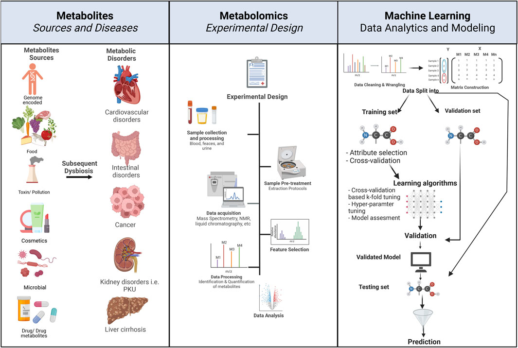
FIGURE 1. Principles of metabolomics experimental design and associated ML workflow. The left panel describes the various sources of metabolites. Metabolite exposure can be through endogenous and exogenous means, e.g., human-encoded, microbiome-encoded, food, drugs, and toxins. Metabolic dysbiosis can be associated with metabolic disorders, e.g., cancer, cardiovascular disease, intestinal disorders, and diabetes. The center panel describes the typical flow and design of a metabolomic experiment, starting with the 1) study design where disease and control groups are determined, 2) followed by sample selection, e.g., urine, stool, blood, and serum, 3) collected samples undergo pre-treatment and processing according to experimental design, 4) data acquisition, e.g., through mass spectrometry or NMR, 5) feature selection involves the identification of desired metabolite features that will undergo subsequent, 6) data processing through the quantification of metabolites, and finally, 7) data analysis depends on the study design. The right panel describes the concepts of ML workflow and prediction, starting with 1) data wrangling and cleaning, 2) matrix construction, where data from each metabolite is placed in a matrix in reference to the conditions, i.e., disease (marked in red), control (marked in blue), 3) data are then divided into testing, validation and training datasets, 4) ML algorithm is applied, and 5) cross-validation, and testing of the predictive power of the algorithm on a test dataset. Created with BioRender.com.

Metabolomics studies can be subclassified into three major approaches: targeted analysis (Shulaev 2006; Griffiths and Wang 2009; Mookherjee et al., 2020), metabolite profiling, i.e., untargeted analysis (Fiehn 2002; Halket et al., 2005), and metabolic fingerprinting, which is also known as exometabolomics and focuses on extracellular metabolites while utilizing analytical profiling approaches (Allen et al., 2003; Mapelli, Olsson, and Nielsen 2008; Silva and Northen 2015; Thomas et al., 2021). Targeted approaches are limited to a set of predetermined metabolites of interest for identifying and quantifying these specific metabolites. Untargeted approaches are conducted to identify a comprehensive metabolic profile in a specimen. The choice of metabolomics workflow and the associated downstream steps depends on the choice of experimental approach (Newgard 2017). Typically, untargeted metabolomics experiments generate substantial volumes of complex data requiring specialized computational processing and interpretation methods. Data interpretation software should ideally be capable of background noise elimination, peak identification and alignment, and peak normalization. While commercial and public domain software packages attempt to perform some of these tasks, there is no universal software for data extraction and analysis software. In metabolomics, hundreds of metabolites are detected and routinely analyzed. The complexity and magnitude of data produced from metabolomic studies necessitate the use of computational methods to analyze the data and elicit potential trends.

Artificial Intelligence (AI), both as a concept and research field, has gained attention across the twenty-first century. With its various applications in understanding the structures or trends in vast amounts of data collected or generated from modern high-throughput experiments, AI and machine learning (ML) offer countless possibilities. ML is used to develop models that can tackle large-scale data and, through learning, can solve complex problems. ML algorithms are fundamentally based on the ability to build mathematical models from a group of sample data (Dhall, Kaur, and Juneja 2020). Typically, a dataset used for developing a machine learning model is divided into a training subset, for example, comprised ∼70% of the available data and used in the ML algorithm to build a model and make predictions, and a testing subset, for example, ∼30% of the data used to provide an unbiased evaluation of the final model from the training step. Often, an intermediate validation step is added to assist in determining the most accurate model and obtaining optimal model hyper-parameters. In this instance, the data can be divided through a 60-20-20 split, where 20% of the data can act as an additional validation set. The initial learning process requires extensive data to allow the ML algorithm more opportunities to learn and improve the model. The ability of the algorithm to learn is formally through a mathematical function that maps specific inputs to certain outputs. The training dataset is used to guide the algorithms to make predictions without being explicitly programmed. This is achieved through a series of operations, where learning is made on the basis of weights and biases that will eventually make predictions in a finite number of steps (Cohen 2021). Having experienced the training dataset where the algorithm was able to learn and build a general model, the next step is testing the model’s performance on an independent dataset that contains previously unseen data and producing sufficiently accurate predictions. Predictions are based on the algorithm’s ability to assign each input to the chosen statistical representation defined by the user. The better the algorithm can learn from the input data provided, the more accurate the algorithm can produce predictions (Antonakoudis et al., 2020; Deepthi et al., 2020).

Constructing an ML model requires a series of steps: 1) Defining the training dataset: it involves identifying the type of data to be used as the training dataset; the input data would change depending on the problem that needs to be addressed. 2) Gathering the training dataset: a representation of the real-world use requires a set of inputs that will address the problem under investigation. 3) Input feature representation: The learned function’s accuracy strongly depends on how the input object is represented. Input objects are transformed into feature vectors, which have several descriptive features. The number of features must be sufficient to contain enough information to predict the output accurately and not too large to affect the dimensionality. 4) Determining the type of algorithm to be used: this is the algorithm that will be used to fit the data during the testing/training phase into a model. The choice of the algorithm depends on several factors, including the question the analysis is trying to answer, the data, and the ML category used, i.e., supervised learning, unsupervised learning, reinforcement learning, and semi-supervised learning (it is expanded upon later). 5) Training the algorithm: running the algorithm on the gathered training dataset; this step might require additional user input depending on the choice of the algorithm. Cross-validation can be used to adjust hyper-parameters (variables that determine how the algorithm is trained, e.g., learning rate, number of branches, clusters, and epochs) and optimize performance on a subset of the training set. 6) Validation: the training phase is often followed by a validation step to fine-tune the hyper-parameters of the classifiers. This validation step is independent of the cross-validation performed on the training set and uses a separate validation dataset. Validation is typically necessary to compare the performance of the different candidate classifiers: it is used to obtain performance parameters, including accuracy, sensitivity, and specificity of the models, and to estimate the models’ prediction error or bias. The model with the best performance on the validation set is then chosen to move forward to the testing phase. 7) Testing and evaluation: after hyper-parameter adjustments and learning, the accuracy of the learned function is assessed through the performance of the algorithm on an entirely new testing dataset, independent of the training and validation dataset (Figure 1: Principles of Metabolomics experimental design and associated ML workflow.).

Model performance assessment is an important step in properly evaluating the validity of a model’s predictions and deciding which model is best for a given problem. Model assessment methods are varied, depend on the characteristics of the problem, and can include a process known as hyper-parameter tuning, where they can be used to control the learning process of the model. The most commonly used assessment methods for classification problems are accuracy (Gajda and Chlebus 2022), cross-entropy (Boubezoul, Paris, and Ouladsine 2008; Gajda and Chlebus 2022), area under the curve (AUC) (Airola et al., 2011; Yala et al., 2019; Gajda and Chlebus 2022), while for regression analysis, mean squared error (Bellet, Habrard, and Sebban 2013), mean absolute error (Airola et al., 2011; Bellet, Habrard, and Sebban 2013) and root mean squared error (Nguyen et al., 2019) are more commonly employed. However, other performance metrics are available, including variance and $R^2$ coefficient, to name a few. Determining model specificity (the ability of a model to identify true negatives correctly) and sensitivity (the ability of a model to correctly identify true positives) (Trevethan 2017) are additional methods that can inform researchers and apply some context to the data under investigation (Parikh et al., 2008; Trevethan 2017).

With every newly discovered metabolite, the field of metabolomics has grown, allowing for a comprehensive assessment of biological specimens and their associated compounds. This improved understanding of the human body at the molecular and biochemical levels is crucial in aiding disease diagnosis and therapeutic development (Gowda et al., 2008). Over the years, the significant contribution of AI and associated applications in various biomedical fields has grown, demonstrating the application of ML in disease prediction and diagnosis of multiple diseases, including cardiovascular disorders, cancer, and rare genetic diseases.

In 2019, an editorial published in Nature titled “Why the metabolism field risks missing out on the AI revolution” expressed concern with the lack of momentum in AI-assisted applications in the field of metabolic research as opposed to other areas, such as genetics, for example. The curation of high-quality datasets, as well as the collective efforts of various institutions and funding bodies over the past few years, has increased the number of AI-assisted metabolomics studies. The number of metabolomic publications with AI and ML-based methods has been consistently on the rise, with very few publications (∼1/year) in the early 2000s, steadily rising to reach ∼150 publications in 2021, and the number of ML-assisted publications in 2022 promising to surpass this. The most used ML methods in metabolomic studies in the past years are RF, SVM, logistic regression, and, more recently, DL (Figure 2).

FIGURE 2

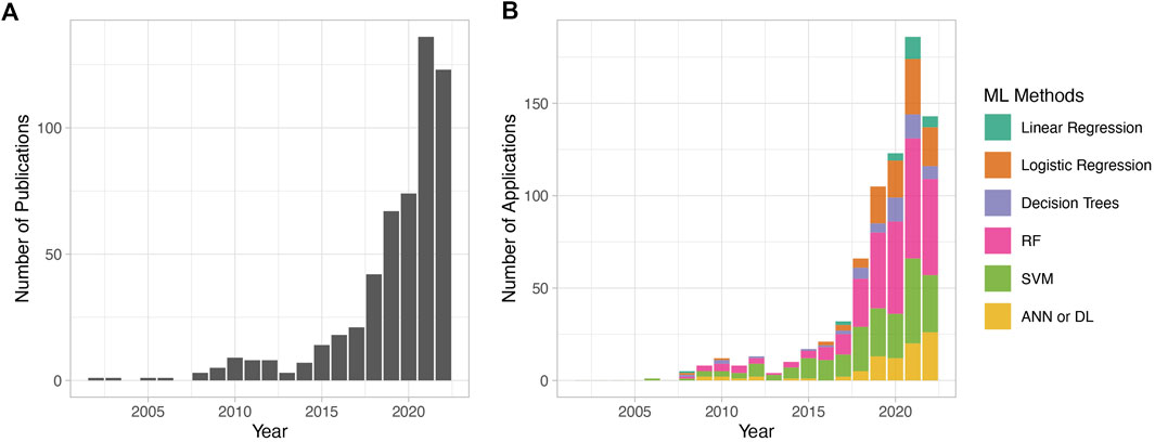
FIGURE 2. Metabolomic publications using machine learning in data analytics over the past 2 decades. PubMed was searched using the keywords “metabolomics” and “machine learning” from 2002 to 2022. Results were manually filtered to remove review articles and irrelevant publications. The counted publications include studies that use any of the mentioned ML algorithms in the context of metabolomic analysis, including classification problems, biomarker discovery, peak identification, metabolomic data analysis tools, and others. Only ML algorithms employed for disease model building are considered. (A) The total number of publications per year. (B) The number of publications using ML methods per year. The y-axis in (A) and (B) are different because in (B), it indicates only the ML methods discussed in this review. The total number of publications across panels (A) and (B) varies because publications often utilize multiple ML algorithms.

The integration of metabolomics with analytical ML techniques can be used to answer questions that other omics approaches cannot answer alone (Gowda et al., 2008; Graham et al., 2018; Turi et al., 2018; Jendoubi 2021). Here, we discuss major ML approaches for analyzing metabolic profiles, focusing on biomarker discovery and disease diagnosis.

Types of machine learning algorithms

ML algorithms can be used to analyze ever-increasing amounts of generated and accumulated data. ML algorithms are traditionally divided into supervised, unsupervised, semi-supervised, and reinforcement learning (Figure 3). For the purposes of this review, we focus on ML algorithms used in metabolomic studies, mainly supervised and unsupervised algorithms. The algorithms highlighted in the following sections do not exclusively belong to any of the mentioned ML categories; rather, the same algorithms can be used for multiple learning categories (e.g., k-Nearest Neighbor can be used in supervised and unsupervised learning).

FIGURE 3

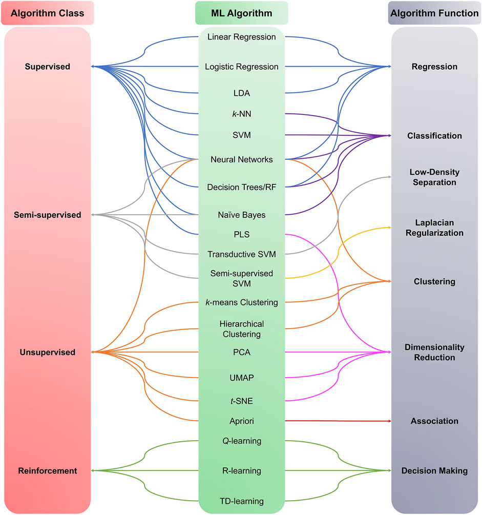
FIGURE 3. Machine learning algorithms categories. ML algorithms are divided into four main classes: Supervised, Unsupervised, Semi-supervised, and Reinforcement learning. The category choice depends on the type and nature of the data under investigation, i.e., labeled or unlabelled data.

Machine learning categories

Supervised learning

Supervised learning involves inferring a function from a labeled dataset input and a specific expected result (output), i.e., an input-output pair. With data containing continuous values, linear regression analysis is commonly used for objectives such as forecasting, prediction, and process optimization (Biswas, Saran, and Wilson 2021). Logistic regression is used with the classification into two categories. Classification for more than two categories can be performed using Support Vector Machines (SVM), decision trees, Random Forest (RF), and other methods (refer to Figure 3).

Unsupervised learning

In unsupervised machine learning, the algorithm learns patterns from unlabeled data. The algorithm takes a dataset with only inputs and attempts to find a structure in the data by grouping or clustering the data points (Dhall, Kaur, and Juneja 2020). Unlike supervised learning, where the algorithm learns from data that has been labeled, classified, or categorized, unsupervised algorithms identify trends or commonalities in the data and respond based on the presence or absence of these commonalities in the data. This analysis can have various goals, from identifying hidden data trends to reducing redundancy, i.e., dimensionality reduction using Uniform Manifold Approximation and Projection (UMAP) (McInnes, Healy, and Melville 2018) and t-distributed stochastic neighbor embedding (t-SNE) (Van Maaten and Hinton 2008), or grouping together similar data (Dhall, Kaur, and Juneja 2020), i.e., clustering. Examples of unsupervised algorithms include k-means clustering, hierarchical clustering, anomaly detection, neural networks (NN), principal component analysis (PCA), independent component analysis (ICA), and apriori algorithms.

Semi-supervised learning

Semi-supervised learning falls between unsupervised and supervised learning. It combines a small amount of labeled data with a large amount of unlabeled data during the training process and uses context to identify data patterns (Dhall, Kaur, and Juneja 2020). For example, this method can be used for classification problems that require a supervised learning algorithm to achieve the end goal; however, it would not require extensive labeling. It is faster than supervised learning because it involves a mixture of labeled and unlabeled data. Examples include generative models, low-density separation, Laplacian regularization, and heuristic approaches. This approach is not commonly used in the field of metabolomics, with few published applications (Libbrecht and Stafford Noble 2015; Migdadi et al., 2021; Abram and Douglas, 2022; Iqbal et al., 2022).

Reinforcement learning

This method was adopted to direct unsupervised ML by rewarding desired behavior and punishing undesired ones. Positive feedback strengthens the model’s ability to connect target inputs and outputs (Dhall, Kaur, and Juneja 2020). Examples include Monte Carlo, Q-learning, State–action–reward–state–action (SARSA), Q-learning Lambda, SARSA-Lambda, and Deep Q-Learning (DQN), to name a few. Reinforcement learning is often converged around fields such as game theory, operations research, and swarm intelligence, as they are highly dependent on using robotics.

On the functional level, different ML algorithms are mainly geared toward solving regression, clustering, or classification problems. A representation of different ML algorithms with functional categorization is depicted in Figure 4, and brief descriptions of the most commonly used ML algorithms are indicated in Table 1. Supervised ML algorithms are by far the most commonly used in the field of metabolomics. For this review, six algorithms centering around supervised learning are highlighted in the following section, and the application of these algorithms to metabolomic data will be expanded upon.

FIGURE 4

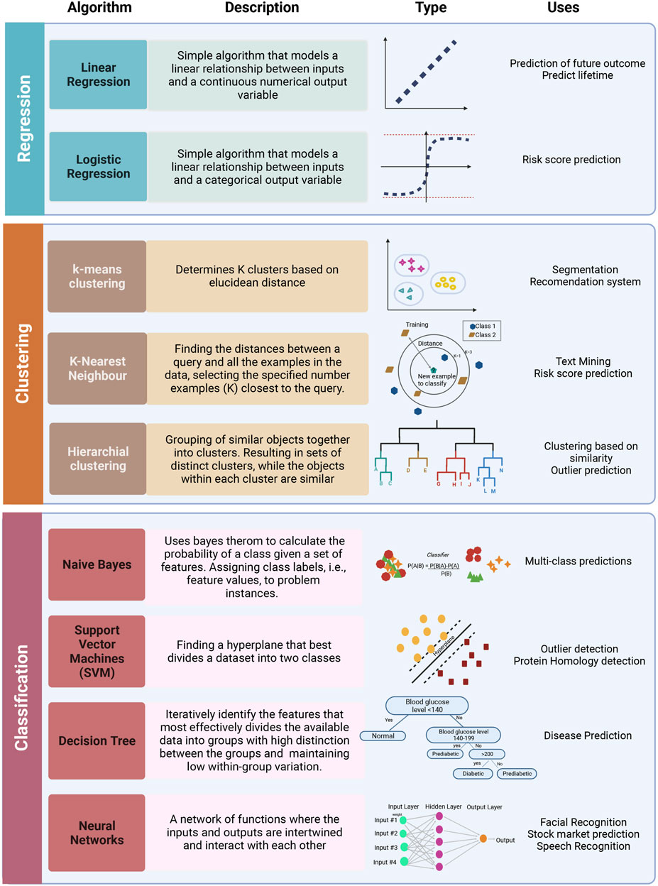
FIGURE 4. Representation of most commonly used ML algorithms with functional categorization accompanied by graphical representations of each algorithm and some potential applications. The most frequently used algorithms can be grouped into regression (linear and logistic), clustering (k-means, k-NN, hierarchical clustering, NN), and classification (Naive Bayes, SVM, Decision trees). Created with BioRender.com.

TABLE 1

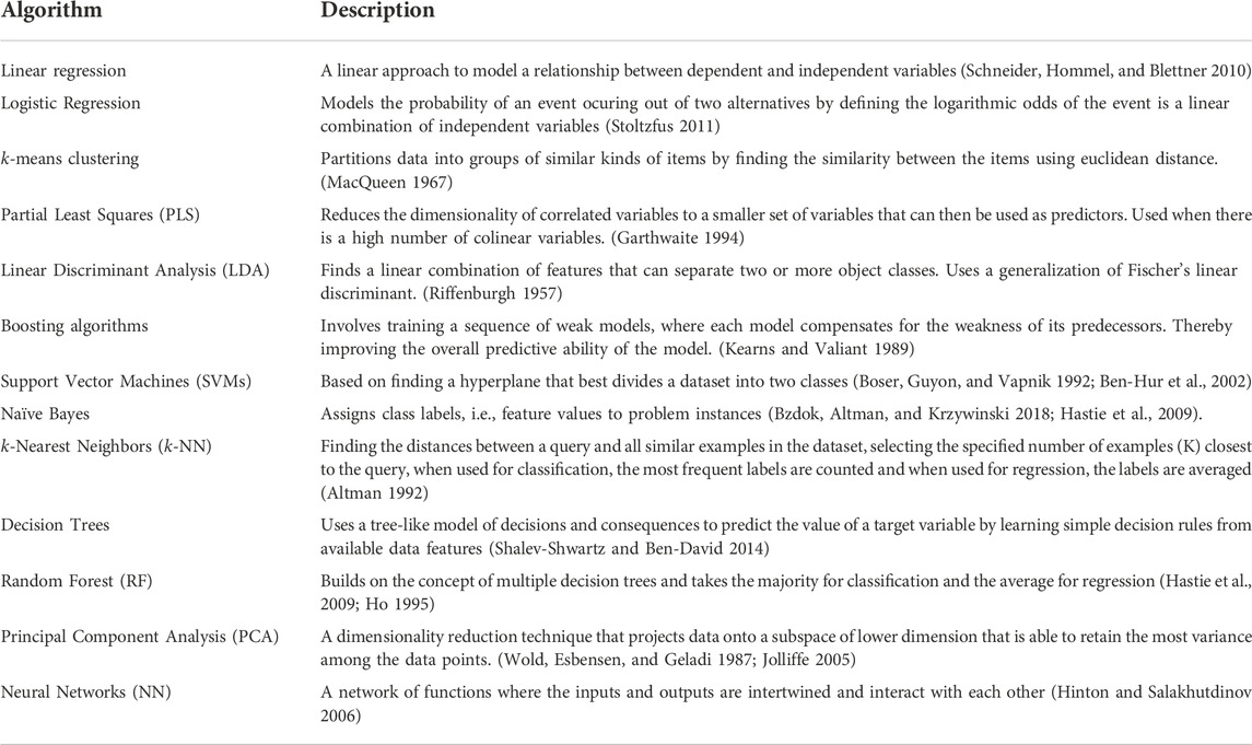
TABLE 1. Key applied machine learning algorithms.

Machine learning algorithms

Regression analysis

Regression analysis is a group of statistical procedures used to estimate the relationship between a dependent variable (outcome or response) and one or more independent variables (predictors, covariates, or features). This method of statistical analysis progressed from the least-squares method to the regression. It can be used in a variety of fields. In order to interpret the output in real-world relationships, a number of assumptions are made, such as that the sample is representative of the entire population and that no errors occurred when measuring the independent variables (Vetter and Schober 2018). Regression analysis is used for two distinct purposes: inferring causal relations between the variables under investigation and prediction (Baumgartner, Böhm, and Baumgartner 2005).

Linear regression

Linear regression models the relationship between dependent and independent variables by fitting a straight line (linear equation) to the observed data (Schneider, Hommel, and Blettner 2010). Predictions based on linear regression are simple: data trend is observed, then a prediction is made on the basis of that trend (Casson and Farmer 2014; Vetter and Schober 2018). While not all data follow a linear trend, linear regression is often the first attempt used to understand data and for predictive analyses.

Logistic regression

A statistical model used to predict a binary outcome (one scenario out of two possible alternatives) based on a set of independent variables (those that influence the outcome) using a logarithmic odds scale (Stoltzfus 2011). Typically, logistic regression analysis is used for classification purposes and when dealing with binary outcomes i.e., two categories.

Decision trees

A statistical decision support tool that uses a tree-like model of decisions and possible consequences. Each tree is similar in structure to that of a flowchart. Each node represents a test, e.g., taking a vitamin, each subsequent branch represents the outcome of the test, i.e., “yes” or “no” for taking the vitamin, and each leaf node represents a class label (Shalev-Shwartz and Ben-David 2014; Kamiński, Jakubczyk, and Szufel 2018). Decision trees consist of three types of nodes: decision, chance, and end nodes (Kamiński, Jakubczyk, and Szufel 2018). Decision trees are constructed to iteratively identify the feature that most effectively divides the available data into groups with a high distinction between the groups in terms of outcome while maintaining a low within-group variation.

Random forest (RF)

A statistical classification method composed of an assembly of many decision trees constructed during the training phase. Generally outperforming decision trees as they correct the observed overfitting. New objects are classified based on the attributes of the data. Each tree is classified and gives a vote for the chosen attribute. When used for classification, the classification with the most votes is chosen, and when used for regression purposes, the average votes are used (Hastie et al., 2009; Dhall, Kaur, and Juneja 2020). RF models are among the most frequently used algorithms for prediction or classification purposes, with various omics applications from understanding the human gut microbiome, differentiating between healthy and disease metabolome, investigating the pregnancy metabolome, cancer diagnosis to the more recent COVID-19 diagnosis and classification of COVID-19 severity. Key studies using these ML algorithms for metabolomic understanding will be highlighted later.

Support vector machines (SVM)

Proposed in 1992 by Boser, Guyon, and Vapnik, SVMs (Boser, Guyon, and Vapnik 1992) has been popular classification tools in many fields, including bioinformatics and biological data analysis in general (Saeys, Inza, and Larrañaga 2007). SVMs split training observations into two classes by constructing a hyperplane, a decision boundary that separates the data points into two classes. The distance between the hyperplane and the nearest data points of each class is called the margin, and the points onto which this margin hits are called the “support vectors”. The SVM is constructed so that the margin on either side of the hyperplane is maximized (Figure 5) (Vapnik 2006). In many cases, the data points cannot be fully segregated. Here, the SVM will try finding a “soft margin” that allows the misclassification of a few points while minimizing the cost of the training points that are on the wrong side of the classification boundary (Cortes and Vapnik 1995).

FIGURE 5

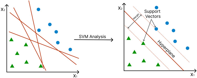
FIGURE 5. Support Vector Machines (SVM) construct a hyperplane to separate data into two classes. Axes represent different features. Green triangles and blue circles represent different conditions (e.g., disease vs. control). The margin (red dotted line) is the distance between the hyperplane and the support vectors (the nearest data point of each class).

In the case of data that are not linearly separable, the data points are mapped into a higher dimensional feature space in which they become linearly separable (Cortes and Vapnik 1995) (Figure 6). This is known as the “kernel trick” and gives SVMs major advantage over other statistical multivariate methods, such as PCA, Partial Least Squares (PLS), and Orthogonal Projections to Latent Structures (OPLS), which cannot be applied to nonlinear cases. A variety of different kernel functions can be employed to transform the data, including the linear kernel, polynomial kernel, sigmoid kernel, and Gaussian radial basis function (RBF) kernel (Powell 1987), (Broomhead and Lowe 1988). A major drawback of SVM is that it is natively restricted to binary classification problems, i.e., it can only discriminate between two classes. However, it does not scale well with large datasets because of its computational complexity.

FIGURE 6

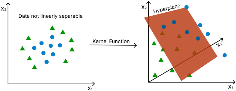
FIGURE 6. The “kernel trick” - non-linearly separable data points are mapped into a higher dimensional feature space in which they become linearly separable. Axes represent different features. Green triangles and blue circles represent different conditions (e.g., disease vs. control). The hyperplane, in this case, becomes a two-dimensional plane.

It is often beneficial to perform feature selection before training multivariate algorithms, such as SVMs, by only selecting subsets of features, in the case of metabolites, on which supervised learning is employed (Guyon 2003). Reducing the number of variables used for model building can simplify the interpretability of the data analysis results and prevent overfitting, which is often caused by non-informative input features (Liu and Motoda 2012). Feature selection methods have been reviewed elsewhere (Miao and Niu 2016). Popular feature selection methods used with SVM models in metabolomics studies include recursive feature elimination (RFE) (Guan et al., 2009; R. Shen et al., 2018), L1 norm SVM (Zhou et al., 2010) (Guan et al., 2009) (Zhou et al., 2010) and variable importance in projection (VIP) ((Zhang et al., 2018), (Cheng et al., 2019) (Z. Chen et al., 2021)).

Deep learning (DL)

Deep learning (LeCun, Bengio, and Hinton 2015) has risen to prominence as the most popular type of machine learning algorithm recently. It uses artificial neural networks (ANN) to construct complex relationships relating input variables to the outcome, advancing classifier performance beyond typical machine learning techniques, particularly in circumstances involving large-scale datasets with high dimensionality. The potential of deep learning is endless; however, it is an intensive process that requires considerable computational power, and its results are often difficult to interpret. In the case of metabolomics studies, it is difficult to evaluate from the model, which features affect classification the most. Deep learning’s recent success has been fueled by an increase in computing power—particularly the introduction of graphics processing units, or GPUs —, as well as the availability of large-scale data sets to use for training the models.

Although there are applications of unsupervised deep learning, including autoencoders (Rumelhart, Hinton, and Williams 1985; Hinton and Salakhutdinov, 2006; Hinton and Salakhutdinov 2006) and generative adversarial networks (Goodfellow et al., 2014 (Goodfellow et al., 2014)), in this review, we focus on supervised deep learning.

An artificial NN is composed of units, termed neurons, that combine multiple inputs and produce a single output. The network approximates the functions that link inputs (e.g., gene expression levels, metabolite concentrations) to desired outputs (e.g., disease risk). Neurons are organized into several layers, with an input layer, an output layer, and intermediate layers, called “hidden layers” (LeCun, Bengio, and Hinton 2015). The variables from the input layer are multiplied by specific values called weights and fed into the neurons of the first hidden layer. Each neuron takes the input, and applies a nonlinear activation function to it, such as sigmoid (Narayan 1997) or rectified linear unit (ReLU) (Glorot et al., 2011), and modifies the outcome by adding a bias to it. The output is then passed on to the next hidden layer. Finally, the outputs of the hidden layers are linearly combined in the output layer and often passed through a classifier function, e.g., a Softmax function, to produce an output value. During supervised NN training, the tunable parameters of the network, i.e., the weights and biases, are optimized so that the distance between the network’s computed outcome and the experimentally determined outcome is minimized (Figure 7).

FIGURE 7

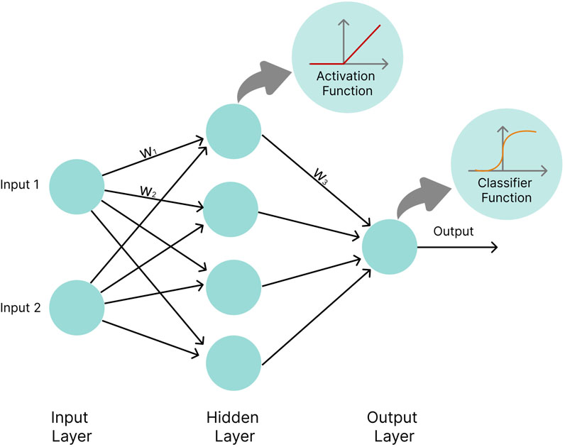
FIGURE 7. Basic neural network architecture. Circles represent neurons. w₁, w_2, and w₃ represent weights by which values calculated inside neurons are multiplied before being passed on to the next layer. In the hidden layer neurons, values are passed into an activation function (e.g., the ReLU function), while the output layer neuron applies a classifier function (e.g., the Softmax function) to input values.

Weights and biases are usually randomly initialized in an artificial neural network and then gradually optimized with the aid of a backpropagation algorithm. A cost function (e.g., the sum of squared errors, cross-entropy) computes the difference between the network’s output and the desired output. The derivative of the cost function with respect to the weight can be used to evaluate how a slight change in a particular weight affects performance. The parameters of the network are adjusted in a direction that minimizes the cost. This process is termed gradient descent because it travels down the slope of the cost function in steps until, optimally, it reaches its global minimum (Figure 8). However, cost functions are often complicated in reality, with many local minima and saddle points to which gradient descent could converge. Since the slope in these regions is also zero, it is almost impossible to escape them. Stochastic gradient descent (Bottou 2010) offers a more efficient approach, in which only a subset (minibatch) of the training data is selected at random and used for cost minimization. Using different mini-batches for each calculation provides enough stochasticity to avoid getting stuck in local minima and saddle points, in addition to drastically reducing computation time and cost.

FIGURE 8

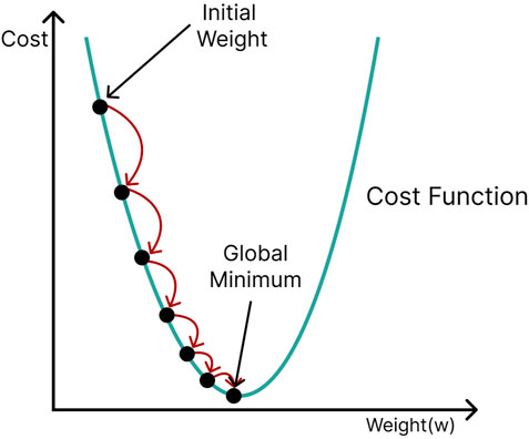
FIGURE 8. Gradient descent; initial network parameters (weights and biases) are adjusted in a direction that travels down the slope of the cost function (green curve) until the minimum is reached.

An artificial NN is considered ‘deep’ when it contains more than one hidden layer. It has been shown that a single hidden layer can approximate any function that maps input patterns to output patterns, given that sufficient neurons are employed (Cybenko 1989), (Hornik, Stinchcombe, and White 1989). However, using more hidden layers improves generalization and leads to more accurate modeling (LeCun, Bengio, and Hinton 2015). Some commonly used types of artificial NN include feed-forward NN, recurrent neural networks, convolutional neural networks (CNN), and deep Boltzmann machines. For an excellent review of NN types, refer to Min et al., 2016 (Min, Lee, and Yoon 2016); for potential applications, refer to (Mendez, Broadhurst, and Reinke 2019; Pomyen et al., 2020).

DL has only recently been used in the analysis of omics data, and the application of DL in metabolomics, in specific, is still emerging and comparatively low compared to other omics. Metabolomic studies that use DL algorithms are, therefore, much fewer than those that utuseilize other ML algorithms.

Use of ML approaches in metabolomic studies

Recently, ML techniques have been used for the analysis of metabolomics data from numerous diseases. For the purposes of this review, we are focusing on key studies that used the aforementioned ML approaches in metabolomic investigations, categorized according to the conditions being studied. For examples of metabolomic studies using ML approaches, refer to Table 2 and Supplementary Table S1.

TABLE 2

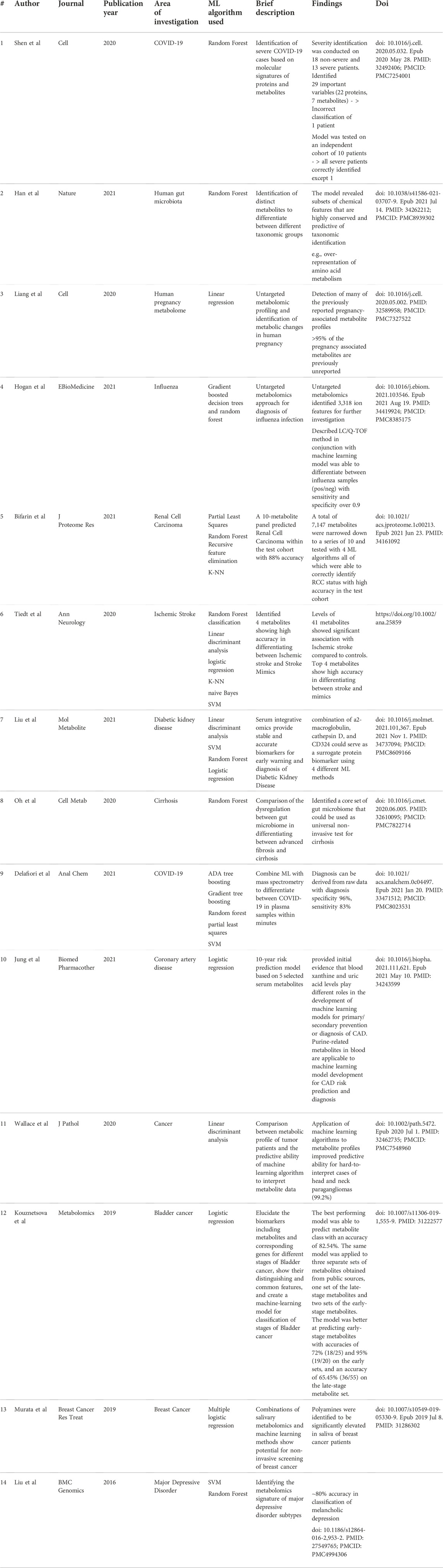
TABLE 2. Examples of metabolomics studies utilizing ML algorithms.

Cancer

Ovarian cancer

In one of the earliest studies, Yu et al. developed an SVM classification model that achieved an average sensitivity of 97.38% and an average specificity of 93.30% for distinguishing cancer from healthy tissue, using a dataset provided by the National Cancer Institute containing serum metabolomic data from ovarian cancer and normal tissue (Yu et al., 2005).

The research group of Guan et al. also extensively studied ovarian cancer metabolites. In 2009, they constructed classifiers using linear and non-linear SVM to diagnose ovarian cancer from serum metabolites with over 90% accuracy, significantly better than a random classifier (Guan et al., 2009).

The same research team published in 2010 (Zhou et al., 2010) how they evaluated a customized fSVM algorithm (SVM for functional data classification (Rossi and Villa 2006)) coupled with ANOVA feature selection for detecting of ovarian cancer using serum metabolites. One of the tested models achieved 100% accuracy in split validation and 98.9% in leave-one-out cross-validation.

In a third study published in 2015 (Gaul et al., 2015), the authors were able to generate a further SVM model capable of identifying early-stage ovarian cancer with 100% accuracy, this time using a panel of sixteen serum metabolites selected by RFE. Eleven of the sixteen metabolites were identified, including phosphatidylinositol, as well as the lysophospholipids lysophosphatidylethanolamine and lysophosphatidylinositol.

Metabolomic analysis has also been found to predict ovarian cancer recurrence. An SVM prediction model was employed by Zhang et al. with ten significant plasma biomarkers, yielding area under the curve (AUC) values reaching 0.964 (Zhang et al., 2018). The results showed a clear clinical advantage over the most commonly used clinical biomarker, CA125, which by contrast, produced an AUC value of only 0.6126.

Breast cancer

An interesting metabolomics study on breast cancer by Henneges et al. focused on modified nucleosides (degradation products of cellular RNA metabolism) and ribosylated metabolites in urine samples (Henneges et al., 2009). From a set of 35 pruned metabolites, 44 pairwise combinations of metabolite features were employed for SVM-based analysis. The sensitivity and specificity of this model were 83.5% and 90.6%, respectively. S-adenosylhomocysteine (SAH) was the most commonly recurring compound in the metabolite pairs, underlining its importance for RNA methylation in cancer pathogenesis.

In another study conducted on breast cancer samples, Alakwaa et al. demonstrated that DL could reliably predict estrogen receptor status (Alakwaa, Chaudhary, and Garmire 2018). The authors used feed-forward networks with a sigmoid activation function and a softmax classifier on a dataset containing 162 metabolites. The predictions were compared to traditional ML methods like RF, SVM, prediction analysis for microarrays (PAMs), generalized boosted models, recursive partitioning and regression trees (RPART), and linear discriminant analysis, with DL models displaying the highest accuracy (AUC 0.93). This DL method also identified eight unique metabolic pathways that seem to promote breast cancer. The study’s findings suggest that DL may be used to deduce the topology of affected biochemical pathways from a network analysis of a metabolomics data set.

The predictive abilities of five potential urinary biomarkers for breast cancer were evaluated by Kim et al. (Kim et al., 2010). Multivariate methods (linear and Gaussian SVM algorithms, decision trees, and RF) were shown to outperform univariate methods by about 6.6–12.7%. It is noteworthy, however, that the linear SVM model scored the lowest in specificity.

Endometrial cancer

Cheng et al. (Cheng et al., 2019) applied 4 ML algorithms- SVM, Partial Least Square-Discriminant Analysis (PLS-DA), RF, and LR-to identify metabolomic biomarkers in cervicovaginal fluid for endometrial cancer detection. The SVM and RF techniques displayed the greatest accuracy of 78% (75% sensitivity and 80% specificity) in the testing dataset.

Hepatocellular carcinoma

Xue et al. (Xue et al., 2008) applied stepwise discriminant analysis (SDA) and SVM algorithms to identify a set of 13 serum metabolites to distinguish between patients with hepatocellular carcinoma and healthy controls with 75% accuracy. The metabolites included carbohydrates, amino acids, fatty acids, cholesterol, and low molecular weight organic acids.

Lung cancer

A more recent study used SVMs with untargeted lipidomics to identify features most important for early-stage lung cancer detection (Wang et al., 2022). Lung plasma lipidomic profiling was carried out on 311 participants using mass spectrometry. Using SVM feature selection, nine lipids were chosen for developing a liquid chromatography-mass spectrometry-based targeted assay. The authors validated the ability of these nine lipids to detect early-stage cancer across multiple independent cohorts, including a hospital-based lung cancer screening cohort of 1,036 participants and a prospective clinical cohort containing 109 participants, in which the assay reached more than 90% sensitivity and 92% specificity. The selected lipids were also shown to be differentially expressed in early-stage lung cancer tissues in situ. This assay, which the authors named “Lung Cancer Artificial Intelligence Detector,” shows promise for the early detection of lung cancer and large-scale screening of high-risk populations for cancer prevention.

Squamous cell carcinoma

In their 2019 study, Hsu et al. uncovered potential metabolic biomarkers for oral cavity squamous cell carcinoma (Hsu et al., 2019). They constructed a three-marker panel consisting of putrescine, glycyl-leucine, and phenylalanine, using an SVM model that can discriminate cancerous from adjacent non-cancerous tissues with high sensitivity and specificity based on receiver operating characteristic (ROC) analysis.

RF and SVM also demonstrated favorable results in the identification of esophageal squamous cell carcinoma tissue based on differential metabolites (Z. Chen et al., 2021). Among the three models evaluated, RF had the highest predictive performance (100%), but required more computational time (8.99 s), compared to PLS and SVM models, which showed similar predictive performance (95%) and similar computational time (1.27 s and 1.11 s). It is of note, however, that the three models prioritized different features.

Non-Hodgkin’s lymphoma

Bueno Duarte et al., 2020, identified a panel of 18 urine metabolites that can differentiate diffuse large B-cell lymphoma patients from healthy individuals with 99.8% accuracy using an SVM model (Duarte et al., 2020).

Renal cell carcinoma

In another cancer study, Bifarin et al. (Bifarin et al., 2021), identified candidate urine metabolic panels for renal cell carcinoma (RCC) as a noninvasive diagnostic assay. Information from patients and controls was gathered and divided into the model and test cohorts. Multiple ML algorithms were used to test the predictive ability. These include RF, KNN, linear kernel SVMs, and RBF kernel SVMs. A total of 7,147 metabolomic features were identified from the NMR and MS platforms. These were then merged and filtered to only those that showed a greater than 1-fold change between the RCC and control samples, and highly positively correlated features were removed. This hybrid model resulted in a selection of 10 metabolites for a panel. RCC status was tested across the used ML models, and all of them were able to predict RCC status accurately.

Osteosarcoma

An RF classifier demonstrated superiority over an SVM model, with an accuracy of 85% versus 81% for the classification of osteosarcoma and benign tumor patients using both X-ray image features and serum metabolomic data (R. Shen et al., 2018).

Non-cancer conditions

Coronavirus disease (COVID-19)

With the onset of the COVID-19 pandemic, research groups across the globe conducted numerous investigations trying to understand if there was any biological reasoning behind disease heterogeneity, in terms of disease severity, presentation, and even mortality rate. For example, Chen et al. (B. Shen et al., 2020) combined proteomic and metabolomic profiles of 31 COVID-19 patients (18 non-sever, 13 severe) to create an ML molecular classifier, which was eventually able to identify potential blood biomarkers for severe COVID-19. The devised RF model identified 29 variables of priority (22 proteins, seven metabolites); this model had a 0.957 AUC in the training set. Subsequent testing of the model against an independent cohort of 10 patients revealed accurate identification of severe COVID-19 patients for all but one of the cohort. The incorrectly identified patients had potential confounding factors, i.e., age, long period of administration of non-traditional medicine, and several comorbidities. The generated classifier was again tested against a model with 29 randomly selected molecules. The randomly generated model exhibited low accuracy when compared with the classifier.

Type 2 diabetes (T2D)

Shomorony et al. (Shomorony et al., 2020) identified a set of cardiometabolic biomarkers beyond the standard clinical biomarkers that can be used to stratify individuals into disease types and stages. Data features from 1,385 diverse modalities (microbiome, genetics, metabolome, advanced imaging) were collected from 1,253 self-assessed healthy individuals. A linear regression ML algorithm was used to identify whether there were any associated covariates. This was then validated through correlation analysis to identify any significant associations between features. Network analysis was performed to determine whether the identified modalities had biomarker signatures that corresponded to underlying biological systems. Finally, using the identified features, cluster analysis was performed to stratify participants into subsets consistent with their respective health status. The findings were validated in an independent cohort of 1,083 females. The authors highlighted several novel biomarkers in diabetes signature and gut microbiome health, i.e., 1-stearoyl-2 dihomo-linoleoyl-GPC and cinnamoyl glycine, respectively.

Nonalcoholic fatty liver disease (NAFLD)

universal gut-microbiome signatures can be used to predict various diseases. This is true for Oh et al. (Oh et al., 2020) who used stool microbiome from 163 nonalcoholic fatty liver (NAFLD) disease patients and applied an RF ML algorithm with a differential abundance analysis to identify microbial and metabolomic signatures to detect cirrhosis and the authors were able to test the generated model and its ability to differentiate between cirrhosis and fibrosis. The model was able to correctly distinguish between the various stages of fibrosis with high accuracy AUC 0.85. The incorporation of further information into the model, i.e., serum AST levels, showed marked improvement in model performance with AUC 0.94.

Perakakis et al. trained models for the non-invasive diagnosis of non-alcoholic steatohepatitis (NASH) and NAFLD (Perakakis et al., 2019) from serum samples. SVM models including 29 lipids or combining lipids with glycans and/or hormones were shown to classify the conditions with 90% accuracy, and a 10-lipid-model could detect liver fibrosis with 98% accuracy.

Acute myocardial ischemia (AMI)

A multilayer perceptron (MLP) neural network-based model achieved superior results in detecting acute myocardial ischemia (AMI) from serum metabolites in a rat model compared to several other classification algorithms, including SVM, RF, Gradient tree boosting (GTB), and LR (Cao et al., 2022). The model achieved accuracy of 96.67% in the rat model and 88.23% in predicting AMI type II in human autopsy cases of sudden cardiac death.

Chronic kidney disease (CKD)

In an attempt to classify chronic kidney disease patients from serum metabolites, Guo et al. (Guo et al., 2019) constructed two NN; a two-layered fully connected multi-layer NN with MLP with 128 neurons in the hidden layer, and a three-layered CNN with 16 and 32 neurons in the two hidden layers, respectively. The MLP achieved accuracy of 90.4%, while the CNN reached accuracy of 90.6%. Both NNs, as well as an SVM model, were outperformed by an RF classifier with 100% accuracy. A possible reason is the rigorous feature reduction steps performed prior to model application; DL methods specialized in the analysis of high-dimensional data and in this study, from thousands of measured metabolites, only five were retained for the final models.

Celiac disease

In one of the earliest and highly cited studies, metabolic signatures of celiac disease, detected by NMR, were used to construct an SVM model able to differentiate celiac disease patients from healthy controls with 83.4% accuracy using serum metabolites and 69.3% using urine metabolites. After a 12-month gluten-free diet, the same model correctly classified all but one of the patients as healthy (Bertini et al., 2009).

Multiple Sclerosis (MS)

Waddington et al. used ML models including SVM, RF, k-NN, decision tree, and least absolute shrinkage and selection operator (LASSO) logistic regression to predict the tendency of multiple sclerosis patients treated with beta interferons to develop anti-drug antibodies (Waddington et al., 2020). Among the five classification models tested for predicting future immunogenicity from serum metabolomics data, SVMs were one of the most successful at differentiating between cases with and without drug resistance.

Major depressive disorder

Metabolomic signatures associated with certain conditions may still persist after disease remission, as shown in a study by Hung et al., 2021. Eight plasma metabolites were identified as significantly differentially-expressed in patients with major depressive disorder (MDD) with full remission compared with healthy controls. These were then used to construct an SVM model capable of differentiating patients with MDD with full remission from healthy controls with predictive accuracy of nearly 85% (Hung et al., 2021).

Schizophrenia

Chen et al. uncovered metabolic biomarkers that can differentiate between schizophrenia patients with violence and those without violence (X. Chen et al., 2020). RF and SVM analyses unveiled ten and five plasma metabolites, respectively. The common metabolites formed a biomarker panel, including the ratio of l-asparagine to l-aspartic acid, vanillylmandelic acid, and glutaric acid, yielding an AUC of 0.808.

Autism spectrum disorders

In a study conducted by Chen et al., urine organic acids were detected in children with autism spectrum disorder (ASD) and combined with three algorithms, PLS-DA, SVM, and eXtreme Gradient Boosting (XGBoost), for the diagnosis of autism (Hung et al., 2021; Q. Chen et al., 2019). The work proved that autism spectrum disorders present with characteristic metabolic biomarkers that can be investigated for diagnosis of the condition as well as for future research on the pathogenesis of autism and possible interventions.

Gestational age

Another application of ML in metabolomics is the investigation of the human pregnancy metabolome conducted by Liang et al. (Liang et al.,. 2020), where the authors were able to identify a series of compounds (460) and associated metabolic pathways (34) that were significantly changed during pregnancy. The authors were able to construct a linear regression model that correlates certain plasma metabolites with time in gestational age; this model is in high accordance with the ultrasound. An additional two to three metabolites were able to identify the time of labor, e.g., prediction of 2, 4, 6, or 8 weeks to the time of delivery.

Methodological studies

The right choice of ML algorithm is a crucial factor for the success of a metabolomics study. Analysis results usually depend more on the data (type, quantity, quality) than the applied algorithm. Complex, multivariate approaches may be suitable for large, multidimensional datasets; however, in the case of simple, linearly separable data, conventional statistical approaches often outperform ML. Therefore, a large number of metabolomic studies make an effort to compare the predictive ability of different ML algorithms to each other, as well as to more traditional statistical methods.

One of the comprehensive comparative studies is the work by Mendez et al. (Mendez, Reinke, and Broadhurst 2019), in which the authors compared 8 ML algorithms, partial least squares regression (PLS), principal component regression (PCR), principal component logistic regression (PCLR), RF, linear kernel SVM, non-linear SVM with RBF, linear and non-linear ANN, for the binary classification of ten clinical metabolomic datasets. As for the ANNs, the linear network was composed of two layers, with a small number of linear neurons in the hidden layer and a single sigmoidal neuron in the output layer. For the non-linear NN, the activation function of the hidden layer neurons was changed to a sigmoidal function. Both networks were implemented using stochastic gradient descent with a binary cross-entropy loss function. The authors expected non-linear machine ML algorithms, especially the DL models, to outperform linear alternatives. Nevertheless, SVM and ANN only slightly surpassed PLS across all datasets, while RF performed poorly. In conclusion, no single DL or ML algorithm could be identified as superior.

In another 2019 study, Vu et al. evaluated the performance of five classification algorithms (PLS, OPLS, Principal component-Linear Discriminant Analysis (PC-LDA), RF, and SVM) using simulated and experimental 1D ¹H NMR spectral data sets (Vu et al., 2019). Datasets with clear group separation were classified equally well by all five models. However, when the data contained subtle differences between classes, OPLS produced the best results, as it was able to identify the useful discriminant features with good classification accuracy. It is noteworthy that although RF and PC-LDA classified the data more accurately than the other models, they achieved so using the wrong discriminant features.

The superiority of SVM and RF classifiers was demonstrated in an evaluation of seven classification techniques using both simulated and real metabolomics datasets (Trainor, DeFilippis, and Rai 2017). In the simulated datasets, the classifiers performed as follows (from least to greatest error): SVM, RF, Naïve Bayes, sparse PLS, ANN, PLS, and k-NN, while SVM and RF consistently outperformed the rest over the real datasets.

Expanding on the gut microbiome, Han et al. (Han et al., 2021) used RF models to identify sets of metabolites that are able to provide taxonomic distinction and classify the origin of microbial supernatants while also providing insights into highly conserved chemical features that are predictive of taxonomic identity. Han et al. were able to construct a chemical standard library-informed metabolomics pipeline that is both customizable and expandable. This method was used to construct an atlas of metabolic activity that can enable functional studies of the gut microbial communities and was validated using RF ML algorithms.

Concluding remarks

In this work, we provided a review of popular ML techniques as well as key studies that have applied them for the stratification of metabolites from various conditions.

RF and SVM have been among the most widely used algorithms in metabolomic studies. Although DL is a comparatively new player in the field, it is undoubtedly paving its way to metabolomics - and generally to the other omics and integrative multi-omics studies - as evident by the growing number of reports that use NNs in metabolomic analyses.

Cancer is by far the most studied condition, with ML algorithms having been applied to the supervised classification of cancer versus control sample sets from metabolic data obtained from various cancer types, including ovarian, breast, endometrial, lung and liver cancer, renal carcinoma, squamous cell carcinomas, osteosarcoma, and lymphomas.

Choosing the appropriate ML algorithm is crucial to the success of a metabolomics study. It is essential for researchers to be informed of the benefits of each ML approach and to choose one that best suits their needs to obtain reliable and interpretable outcomes. However, after reviewing a number of studies that compared different ML methods, no specific conclusion can be drawn regarding the choice of the algorithm. ML methods that produce good results in some investigations might perform poorly in others. The dimensionality, quality, and characteristics of input data and appropriate feature selection techniques play a significant role in the performance and behavior of the ML methods and their outcomes.

In addition, the choice of hyper-parameters and how they are tuned can influence the results remarkably. Accordingly, a detailed methodology for selecting the most suitable ML algorithm is a topic that needs further investigation. However, we can offer some insight into the pros and cons of each of the popular algorithms discussed in this review, as well as some suggested recommendations regarding their applications within the metabolomics field (Table 3) (Kell 2005; Kourou et al., 2015; Libbrecht and Stafford Noble, 2015; Soofi and Awan 2017; Malakar et al., 2018; Shinde and Shah 2018; Liebal et al., 2020).

TABLE 3

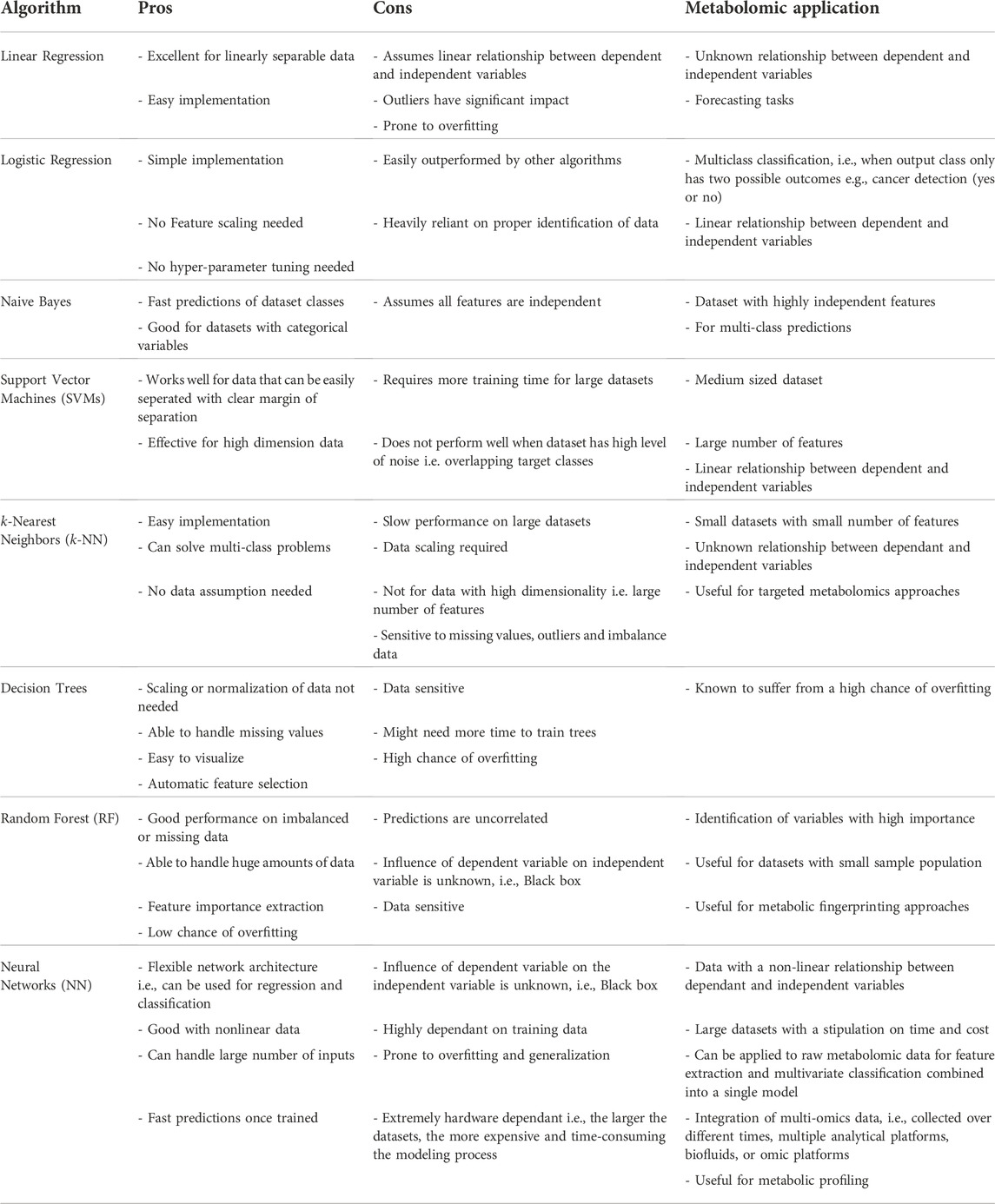
TABLE 3. Pros and cons of ML algorithms and applicability within the field of metabolomics.

Significantly altered metabolites generated by metabolomic experiments and unveiled by machine learning approaches can serve as a starting point for a number of investigations. Biomarker discovery is a definite main target. Nevertheless, their actual predictive ability needs to be further experimentally validated. Further investigations like enrichment studies and pathway analysis can provide new insights into the roles the identified metabolites play in the pathophysiology of various conditions. Additionally, the feasibility of targeting specific metabolites for disease treatment can be explored.

It is noteworthy that most of the reviewed work was published within the last 5 years, which aligns with the obvious rise in popularity ML has gained in recent years, enabled by an increase in computation power, efficiency and accessibility of ML tools, familiarity with the field and abundance of data. As more and large metabolomic data sets become available, it is expected that ML techniques, especially DL, will play a bigger role in building informative and predictive models that can be used to provide high-definition, personalized clinical diagnosis, and treatment.

Author contributions

AM planned and supervised the project. AG and MT wrote the manuscript draft and created the visualizations. AM, AG, and MT reviewed and edited the final manuscript.

Funding

AG was supported by the Mohamed Bin Abdulkarim Allehedan Ph.D. fellowship. MT was partially supported by the American University in Cairo Laboratory Fellowship. AM was partially supported by the American University in Cairo Centennial Grant.

Conflict of interest

The authors declare that the research was conducted in the absence of any commercial or financial relationships that could be construed as a potential conflict of interest.

Publisher’s note

All claims expressed in this article are solely those of the authors and do not necessarily represent those of their affiliated organizations, or those of the publisher, the editors and the reviewers. Any product that may be evaluated in this article, or claim that may be made by its manufacturer, is not guaranteed or endorsed by the publisher.

Supplementary material

The Supplementary Material for this article can be found online at: https://www.frontiersin.org/articles/10.3389/fgene.2022.1017340/full#supplementary-material

References

Abram, K. J., and McCloskey, D. (2022). A comprehensive evaluation of metabolomics data preprocessing methods for deep learning. Metabolites 12 (3), 202. doi:10.3390/metabo12030202

PubMed Abstract | CrossRef Full Text | Google Scholar

Aderemi, A. V., Ayeleso, A. O., Oyedapo, O. O., and Mukwevho, E. (2021). Metabolomics: A scoping review of its role as a tool for disease biomarker discovery in selected non-communicable diseases. Metabolites 11 (7), 418. doi:10.3390/metabo11070418

PubMed Abstract | CrossRef Full Text | Google Scholar

Ahola-Olli, A. V., Mustelin, L., Kalimeri, M., Kettunen, J., Jokelainen, J., Auvinen, J., et al. (2019). Circulating metabolites and the risk of type 2 diabetes: A prospective study of 11, 896 young adults from four Finnish cohorts. Diabetologia 62 (12), 2298–2309. doi:10.1007/s00125-019-05001-w

PubMed Abstract | CrossRef Full Text | Google Scholar

Airola, A., Pahikkala, T., Waegeman, W., De Baets, B., and Salakoski, T. (2011). An experimental comparison of cross-validation techniques for estimating the area under the ROC curve. Comput. Statistics Data Analysis 55 (4), 1828–1844. doi:10.1016/j.csda.2010.11.018

CrossRef Full Text | Google Scholar

Alakwaa, F. M., Chaudhary, K., and Garmire, L. X. (2018). Deep learning accurately predicts estrogen receptor status in breast cancer metabolomics data. J. Proteome Res. 17 (1), 337–347. doi:10.1021/acs.jproteome.7b00595

PubMed Abstract | CrossRef Full Text | Google Scholar

Allen, J., Davey, H. M., Broadhurst, D., Heald, J. K., Rowland, J. J., Oliver, S. G., et al. (2003). High-throughput classification of yeast mutants for functional Genomics using metabolic footprinting. Nat. Biotechnol. 21 (6), 692–696. doi:10.1038/nbt823

PubMed Abstract | CrossRef Full Text | Google Scholar

Altman, N. S. (1992). An introduction to kernel and nearest-neighbor nonparametric regression. Am. Statistician 46 (3), 175–185. doi:10.2307/2685209

CrossRef Full Text | Google Scholar

Antonakoudis, A., Barbosa, R., Kotidis, P., and Kontoravdi, C. (2020). The era of big data: Genome-scale modelling meets machine learning. Comput. Struct. Biotechnol. J. 18, 3287–3300. doi:10.1016/j.csbj.2020.10.011

PubMed Abstract | CrossRef Full Text | Google Scholar

Baumgartner, C., Böhm, C., and Baumgartner, D. (2005). Modelling of classification rules on metabolic patterns including machine learning and expert knowledge. J. Biomed. Inf. 38 (2), 89–98. doi:10.1016/j.jbi.2004.08.009

PubMed Abstract | CrossRef Full Text | Google Scholar

Bellet, A., Habrard, A., and Sebban, M. (2013). “A survey on metric learning for feature vectors and structured data.” arXiv [cs.LG]. arXiv. Available at: http://arxiv.org/abs/1306.6709.

Google Scholar

Ben-Hur, A., Horn, D., Siegelmann, H. T., and Vapnik, V. (2002). Support vector clustering. J. Mach. Learn. Res. JMLR 2, 125–137.

Google Scholar

Bertini, I., Calabrò, A., De Carli, V., Luchinat, C., Nepi, S., Porfirio, B., et al. (2009). The metabonomic signature of celiac disease. J. Proteome Res. 8 (1), 170–177. doi:10.1021/pr800548z

PubMed Abstract | CrossRef Full Text | Google Scholar

Bifarin, O. O., Gaul, D. A., Sah, S., Arnold, R. S., Ogan, K., Master, V. A., et al. (2021). Machine learning-enabled renal cell carcinoma status prediction using multiplatform urine-based metabolomics. J. Proteome Res. 20 (7), 3629–3641. doi:10.1021/acs.jproteome.1c00213

PubMed Abstract | CrossRef Full Text | Google Scholar

Biswas, A., Saran, I., and Perry Wilson, F. (2021). Introduction to supervised machine learning. Kidney360 2 (5), 878–880. doi:10.34067/KID.0000182021

PubMed Abstract | CrossRef Full Text | Google Scholar

Boser, B. E., Guyon, I. M., and Vapnik, V. N. (1992). “A training algorithm for optimal margin classifiers,” in Proceedings of the Fifth Annual Workshop on Computational Learning Theory - COLT. doi:10.1145/130385.13040192

CrossRef Full Text | Google Scholar

Bottou, L. (2010). “Large-scale machine learning with stochastic gradient descent,” in Proceedings of the COMPSTAT’2010. Physica-Verlag HD. Editors Y. Lechevallier, and G. Saporta. doi:10.1007/978-3-7908-2604-3_16

CrossRef Full Text | Google Scholar

Boubezoul, A., Paris, S., and Ouladsine, M. (2008). Application of the cross entropy method to the GLVQ algorithm. Pattern Recognit. 41 (10), 3173–3178. doi:10.1016/j.patcog.2008.03.016

CrossRef Full Text | Google Scholar

Broomhead, D., and Lowe, D. (1988). Multivariable functional interpolation and adaptive networks. Complex Syst. 2, 321–355.

Google Scholar

Bzdok, D., Altman, N., and Martin, K. (2018). Statistics versus machine learning. Nat. Methods 15 (4), 233–234. doi:10.1038/nmeth.4642

PubMed Abstract | CrossRef Full Text | Google Scholar

Cao, J., Li, J., Gu, Z., Niu, J-J., An, G-S., Jin, Q-Q., et al. (2022). Combined metabolomics and machine learning algorithms to explore metabolic biomarkers for diagnosis of acute myocardial ischemia. Int. J. Leg. Med. doi:10.1007/s00414-022-02816-y

CrossRef Full Text | Google Scholar

Casson, R. J., and Farmer, L. D. M. (2014). Understanding and checking the assumptions of linear regression: A primer for medical researchers. Clin. Exp. Ophthalmol. 42 (6), 590–596. doi:10.1111/ceo.12358

PubMed Abstract | CrossRef Full Text | Google Scholar

Cavus, E., Karakas, M., Ojeda, F. M., Kontto, J., Veronesi, G., Ferrario, M. M., et al. (2019). Association of circulating metabolites with risk of coronary heart disease in a European population: Results from the biomarkers for cardiovascular risk assessment in europe (BiomarCaRE) consortium. JAMA Cardiol. 4 (12), 1270–1279. doi:10.1001/jamacardio.2019.4130

PubMed Abstract | CrossRef Full Text | Google Scholar

Chen, Q., Qiao, Y., Xu, X-J., You, X., and Tao, Y. (2019). Urine organic acids as potential biomarkers for autism-spectrum disorder in Chinese children. Front. Cell. Neurosci. 13, 150. doi:10.3389/fncel.2019.00150

PubMed Abstract | CrossRef Full Text | Google Scholar

Chen, X., Xu, J., Tang, J., Dai, X., Huang, H., Cao, R., et al. (2020). Dysregulation of amino acids and lipids metabolism in schizophrenia with violence. BMC Psychiatry 20 (1), 97. doi:10.1186/s12888-020-02499-y

PubMed Abstract | CrossRef Full Text | Google Scholar

Chen, Z., Gao, Y., Huang, X., Yao, Y., Chen, K., Su, Z., et al. (2021). Tissue-based metabolomics reveals metabolic biomarkers and potential therapeutic targets for esophageal squamous cell carcinoma. J. Pharm. Biomed. Anal. 197, 113937. doi:10.1016/j.jpba.2021.113937

PubMed Abstract | CrossRef Full Text | Google Scholar

Cheng, S-C., Chen, K., Chiu, C-Y., Lu, K-Y., Lu, H-Y., Chiang, M-H., et al. (2019). Metabolomic biomarkers in cervicovaginal fluid for detecting endometrial cancer through nuclear magnetic resonance spectroscopy. Metabolomics 15 (11), 146. doi:10.1007/s11306-019-1609-z

PubMed Abstract | CrossRef Full Text | Google Scholar

Cohen, S. (2021). “Chapter 1 - the evolution of machine learning: Past, present, and future,” in Artificial intelligence and deep learning in pathology. 1–12. Editor S. Cohen (Elsevier).

Google Scholar

Cortes, C., and Vapnik, V. (1995). Support-vector networks. Mach. Learn. 20 (3), 273–297. doi:10.1007/bf00994018

CrossRef Full Text | Google Scholar

Cybenko, G. (1989). Approximation by superpositions of a sigmoidal function. Math. Control Signal. Syst. 2 (4), 303–314. doi:10.1007/bf02551274

CrossRef Full Text | Google Scholar

Deepthi, Y., Pavan Kalyan, K., Vyas, M., Radhika, K., Babu, D. K., and Krishna Rao, N. V. (2020). “Disease prediction based on symptoms using machine learning,” in Energy systems, drives and automations (Singapore: Springer), 561–569.

CrossRef Full Text | Google Scholar

Dettmer, K., Aronov, P. A., and Hammock, B. D. (2007). Mass spectrometry-based metabolomics. Mass Spectrom. Rev. 26 (1), 51–78. doi:10.1002/mas.20108

PubMed Abstract | CrossRef Full Text | Google Scholar

Dhall, D., Kaur, R., and Juneja, M. (2020). “Machine learning: A review of the algorithms and its applications,” in Proceedings of ICRIC 2019 (Springer International Publishing).47–63

PubMed Abstract | CrossRef Full Text | Google Scholar

Duarte, G. H. B., Fernandes, A. A. D. P., Silva, A. A. R., Zamora-Obando, H. R., Amaral, A. G., Mesquita, A. D. S., et al. (2020). Gas chromatography-mass spectrometry untargeted profiling of non-hodgkin’s lymphoma urinary metabolite markers. Anal. Bioanal. Chem. 412 (27), 7469–7480. doi:10.1007/s00216-020-02881-5

PubMed Abstract | CrossRef Full Text | Google Scholar

Fiehn, O. (2002). Metabolomics-the link between genotypes and phenotypes. Plant Mol. Biol. 48 (1-2), 155–171. doi:10.1023/a:1013713905833

PubMed Abstract | CrossRef Full Text | Google Scholar

Friedrich, N. (2012). Metabolomics in diabetes research. J. Endocrinol. 215 (1), 29–42. doi:10.1530/JOE-12-0120

PubMed Abstract | CrossRef Full Text | Google Scholar

Gajda, S., and Chlebus, M. (2022). A probability-based models ranking approach: An alternative method of machine-learning model performance assessment. Sensors 22 (17), 6361. doi:10.3390/s22176361

PubMed Abstract | CrossRef Full Text | Google Scholar

Garthwaite, P. H. (1994). An interpretation of partial least squares. J. Am. Stat. Assoc. 89 (425), 122–127. doi:10.1080/01621459.1994.10476452

CrossRef Full Text | Google Scholar

Gates, S. C., and Sweeley, C. C. (1978). Quantitative metabolic profiling based on gas chromatography. Clin. Chem. 24 (10), 1663–1673. doi:10.1093/clinchem/24.10.1663

PubMed Abstract | CrossRef Full Text | Google Scholar

Gaul, D. A., Mezencev, R., Long, T. Q., Jones, C. M., Benigno, B. B., Gray, A., et al. (2015). Highly-accurate metabolomic detection of early-stage ovarian cancer. Sci. Rep. 5 (1), 16351–16357. doi:10.1038/srep16351

PubMed Abstract | CrossRef Full Text | Google Scholar

Glorot, X., Antoine, B., and Bengio, Y. (2011). “Deep sparse rectifier neural networks,” in JMLR Workshop and Conference Proceedings. Available at: https://proceedings.mlr.press/v15/glorot11a.html.

Google Scholar

Goodfellow, I., Pouget-Abadie, J., Mirza, M., Xu, B., Warde-Farley, D., Ozair, S., et al. (2014). Generative adversarial nets. Adv. Neural Inf. Process. Syst. 27. Available at: https://proceedings.neurips.cc/paper/5423-generative-adversarial-nets. doi:10.1145/3422622

CrossRef Full Text | Google Scholar

Gowd, G. A. N., Zhang, S., Gu, H., Vincent, A., Shanaiah, N., and Raftery, D. (2008). Metabolomics-based methods for early disease diagnostics. Expert Rev. Mol. diagn. 8 (5), 617–633. doi:10.1586/14737159.8.5.617

PubMed Abstract | CrossRef Full Text | Google Scholar

Graham, E., Lee, J., Price, M., Tarailo-Graovac, M., Matthews, A., Engelke, U., et al. (2018). Integration of Genomics and metabolomics for prioritization of rare disease variants: A 2018 literature review. J. Inherit. Metab. Dis. 41 (3), 435–445. doi:10.1007/s10545-018-0139-6

PubMed Abstract | CrossRef Full Text | Google Scholar

Griffiths, W. J., and Wang., Y. (2009). Mass spectrometry: From proteomics to metabolomics and lipidomics. Chem. Soc. Rev. 38 (7), 1882–1896. doi:10.1039/b618553n

PubMed Abstract | CrossRef Full Text | Google Scholar

Guan, W., Zhou, M., Hampton, C. Y., Benigno, B. B., Deette Walker, L., Gray, A., et al. (2009). Ovarian cancer detection from metabolomic liquid chromatography/mass spectrometry data by support vector machines. BMC Bioinforma. 10 (1), 259–315. doi:10.1186/1471-2105-10-259

PubMed Abstract | CrossRef Full Text | Google Scholar

Guasch-Ferré, M., Hruby, A., Toledo, E., Clish, C. B., Martínez-González, M. A., Salas-Salvadó, J., et al. (2016). Metabolomics in prediabetes and diabetes: A systematic review and meta-analysis. Diabetes Care 39 (5), 833–846. doi:10.2337/dc15-2251

PubMed Abstract | CrossRef Full Text | Google Scholar

Guijas, C., Rafael Montenegro-Burke, J., Domingo-Almenara, X., Palermo, A., Warth, B., Hermann, G., et al. (2018). Metlin: A technology platform for identifying knowns and unknowns. Anal. Chem. 90 (5), 3156–3164. doi:10.1021/acs.analchem.7b04424

PubMed Abstract | CrossRef Full Text | Google Scholar

Guo, Y., Hui, Y., Chen, D., and Zhao, Y-Y. (2019). Machine learning distilled metabolite biomarkers for early stage renal injury. Metabolomics 16 (1), 4. doi:10.1007/s11306-019-1624-0

PubMed Abstract | CrossRef Full Text | Google Scholar

Guyon, I. (2003). An introduction to variable and feature selection. J. Mach. Learn. Res. Available at: http://citeseer.ist.psu.edu/viewdoc/summary?

Google Scholar

Halket, J. M., Waterman, D., Przyborowska, A. M., Patel, R. K. P., Fraser, P. D., and Bramley, P. M. (2005). Chemical derivatization and mass spectral libraries in metabolic profiling by GC/MS and LC/MS/MS. J. Exp. Bot. 56 (410), 219–243. doi:10.1093/jxb/eri069

PubMed Abstract | CrossRef Full Text | Google Scholar

Han, S., Van Treuren, W., Fischer, C. R., Merrill, B. D., DeFelice, B. C., Sanchez, J. M., et al. (2021). A metabolomics pipeline for the mechanistic interrogation of the gut microbiome. Nature 595 (7867), 415–420. doi:10.1038/s41586-021-03707-9

PubMed Abstract | CrossRef Full Text | Google Scholar

Hasin, Y., Marcus, S., and Lusis, A. (2017). Multi-omics approaches to disease. Genome Biol. 18 (1), 83. doi:10.1186/s13059-017-1215-1

PubMed Abstract | CrossRef Full Text | Google Scholar

Hastie, T., Tibshirani, R., and Friedman, J. (2009). “The Elements of statistical learning” in Springer Series in Statistics. doi:10.1007/978-0-387-84858-7

CrossRef Full Text | Google Scholar

Henneges, C., Bullinger, D., Fux, R., Friese, N., Seeger, H., Neubauer, H., et al. (2009). Prediction of breast cancer by profiling of urinary RNA metabolites using support vector machine-based feature selection. BMC Cancer 9, 104. doi:10.1186/1471-2407-9-104

PubMed Abstract | CrossRef Full Text | Google Scholar

Hinton, G. E., and Salakhutdinov, R. R. (2006). Reducing the dimensionality of data with neural networks. Science 313 (5786), 504–507. doi:10.1126/science.1127647

PubMed Abstract | CrossRef Full Text | Google Scholar

Ho, T. K. (1995). Random decision Forests. Proc. 3rd Int. Conf. Document Analysis Recognit. 11, 278–282.

Google Scholar

Hornik, K., Stinchcombe, M., and White, H. (1989). Multilayer feedforward networks are universal approximators. Neural Netw. 2 (5), 359–366. doi:10.1016/0893-6080(89)90020-8

CrossRef Full Text | Google Scholar

Hou, X-W., Wang, Y., and Pan, C-W. (2021). Metabolomics in diabetic retinopathy: A systematic review. Invest. Ophthalmol. Vis. Sci. 62 (10), 4. doi:10.1167/iovs.62.10.4

PubMed Abstract | CrossRef Full Text | Google Scholar

Hsu, C-W., Chen, Y-T., Hsieh, Y-J., Chang, K-P., Hsueh, P-C., Chen, T-W., et al. (2019). Integrated analyses utilizing metabolomics and transcriptomics reveal perturbation of the polyamine pathway in oral cavity squamous cell carcinoma. Anal. Chim. Acta 1050, 113–122. doi:10.1016/j.aca.2018.10.070

PubMed Abstract | CrossRef Full Text | Google Scholar

Hung, I., Lin, G., Chiang, M-H., and Chiu, C-Y. (2021). Metabolomics-based discrimination of patients with remitted depression from healthy controls using 1H-NMR spectroscopy. Sci. Rep. 11 (1), 15608. doi:10.1038/s41598-021-95221-1

PubMed Abstract | CrossRef Full Text | Google Scholar

Iida, M., Harada, S., and Takebayashi, T. (2019). Application of metabolomics to epidemiological studies of atherosclerosis and cardiovascular disease. J. Atheroscler. Thromb. 26 (9), 747–757. doi:10.5551/jat.RV17036

PubMed Abstract | CrossRef Full Text | Google Scholar

Iqbal, T., Elahi, A., Wijns, W., and Shahzad, A. (2022). Exploring unsupervised machine learning classification methods for physiological stress detection. Front. Med. Technol. 4, 782756. doi:10.3389/fmedt.2022.782756

PubMed Abstract | CrossRef Full Text | Google Scholar

Jendoubi, T. (2021). Approaches to integrating metabolomics and multi-omics data: A primer. Metabolites 11 (3), 184. doi:10.3390/metabo11030184

PubMed Abstract | CrossRef Full Text | Google Scholar

Jolliffe, I. (2005). “Principal component analysis,” in Encyclopedia of statistics in behavioral science (Chichester, UK: John Wiley & Sons). doi:10.1002/0470013192.bsa501

CrossRef Full Text | Google Scholar

Kamiński, B., Jakubczyk, M., and Szufel, P. (2018). A framework for sensitivity analysis of decision trees. Cent. Eur. J. Oper. Res. 26 (1), 135–159. doi:10.1007/s10100-017-0479-6

PubMed Abstract | CrossRef Full Text | Google Scholar

Kearns, M., and Valiant, L. G. (1989). “Crytographic limitations on learning boolean formulae and finite automata,” in Proceedings of the Twenty-First Annual ACM Symposium on Theory of Computing (New York, NY, USA: Association for Computing Machinery). STOC ’89.433–44

PubMed Abstract | CrossRef Full Text | Google Scholar

Kell, D. B. (2005). Metabolomics, machine learning and modelling: Towards an understanding of the language of cells. Biochem. Soc. Trans. 33 (3), 520–524. doi:10.1042/BST0330520

PubMed Abstract | CrossRef Full Text | Google Scholar

Kim, Y., Koo, I., Jung, B. H., Chung, B. C., and Lee, D. (2010). Multivariate classification of urine metabolome profiles for breast cancer diagnosis. BMC Bioinforma. 11, S4. doi:10.1186/1471-2105-11-S2-S4

PubMed Abstract | CrossRef Full Text | Google Scholar

Kourou, K., Exarchos, T. P., Exarchos, K. P., Karamouzis, M. V., and Fotiadis, D. I. (2015). Machine learning applications in cancer prognosis and prediction. Comput. Struct. Biotechnol. J. 13, 8–17. doi:10.1016/j.csbj.2014.11.005

PubMed Abstract | CrossRef Full Text | Google Scholar

LeCun, Y., Bengio, Y., and Hinton, G. (2015). Deep learning. Nature 521 (7553), 436–444. doi:10.1038/nature14539

PubMed Abstract | CrossRef Full Text | Google Scholar

Liang, L., Rasmussen, M-L. H., Piening, B., Shen, X., Chen, S., Röst, H., et al. (2020). Metabolic dynamics and prediction of gestational age and time to delivery in pregnant women. Cell 181 (7), 1680–1692. e15. doi:10.1016/j.cell.2020.05.002

PubMed Abstract | CrossRef Full Text | Google Scholar

Libbrecht, M. W., and Stafford Noble, W. (2015). Machine learning applications in genetics and Genomics. Nat. Rev. Genet. 16 (6), 321–332. doi:10.1038/nrg3920

PubMed Abstract | CrossRef Full Text | Google Scholar

Liebal, U. W., Phan, A. N. T., Sudhakar, M., Raman, K., and Blank, L. M. (2020). Machine learning applications for mass spectrometry-based metabolomics. Metabolites 10 (6), E243. doi:10.3390/metabo10060243

PubMed Abstract | CrossRef Full Text | Google Scholar

Liu, H., and Motoda, H. (2012), Feature extraction, construction and selection: A data mining perspective. in The springer international series in engineering and computer science (New York, NY: Springer), 453.

Google Scholar

Maaten, L. V. D., and Hinton, G. (2008). Visualizing data using T-SNE. J. Mach. Learn. Res. JMLR. Available at: https://www.jmlr.org/papers/volume9/vandermaaten08a/vandermaaten08a.pdf?fbcl.

Google Scholar

MacQueen, J. (1967)., 5.1. Berkeley, CA: University of California Press, 281–298.Some methods for classification and analysis of multivariate observationsProc. Fifth Berkeley Symposium Math. Statistics Probab.

Google Scholar

Malakar, P., Balaprakash, P., Vishwanath, V., Morozov, V., and Kumaran, K. (2018). “Benchmarking machine learning methods for performance modeling of scientific applications,” in 2018 IEEE/ACM Performance Modeling, Benchmarking and Simulation of High Performance Computer Systems, Dallas, TX, USA, 12-12 November 2018 (PMBS).33–44. doi:10.1109/PMBS.2018.8641686

PubMed Abstract | CrossRef Full Text | Google Scholar

Mapelli, V., Olsson, L., and Nielsen, J. (2008). Metabolic footprinting in microbiology: Methods and applications in functional Genomics and biotechnology. Trends Biotechnol. 26 (9), 490–497. doi:10.1016/j.tibtech.2008.05.008

PubMed Abstract | CrossRef Full Text | Google Scholar

McGranaghan, P., Saxena, A., Rubens, M., Radenkovic, J., Bach, D., Schleußner, L., et al. (2020). Predictive value of metabolomic biomarkers for cardiovascular disease risk: A systematic review and meta-analysis. Biomarkers 25 (2), 101–111. doi:10.1080/1354750X.2020.1716073

PubMed Abstract | CrossRef Full Text | Google Scholar

McInnes, Le, Healy, J., and James, M. (2018). “Umap: Uniform Manifold approximation and projection for dimension reduction.” arXiv [stat.ML]. arXivAvailable at: http://arxiv.org/abs/1802.03426.

Google Scholar

Mendez, K. M., Broadhurst, D. I., and Reinke, S. N. (2019). The application of artificial neural networks in metabolomics: A historical perspective. Metabolomics: Official journal of the Metabolomic Society 15 (11), 142. doi:10.1007/s11306-019-1608-0

PubMed Abstract | CrossRef Full Text | Google Scholar

Mendez, K. M., Reinke, S. N., and Broadhurst, D. I. (2019). A comparative evaluation of the generalised predictive ability of eight machine learning algorithms across ten clinical metabolomics data sets for binary classification. Metabolomics 15 (12), 150. doi:10.1007/s11306-019-1612-4

PubMed Abstract | CrossRef Full Text | Google Scholar

Miao, J., and Niu, L. (2016). A survey on feature selection. Procedia Comput. Sci. 91 (1), 919–926. doi:10.1016/j.procs.2016.07.111

CrossRef Full Text | Google Scholar

Migdadi, L., Lambert, J., Ahmad, T., Roland, H., and Wöhler, C. (2021). Automated metabolic assignment: Semi-supervised learning in metabolic analysis employing two dimensional nuclear magnetic resonance (NMR). Comput. Struct. Biotechnol. J. 19 (8), 5047–5058. doi:10.1016/j.csbj.2021.08.048

PubMed Abstract | CrossRef Full Text | Google Scholar

Min, S., Lee, B., and Yoon, S. (2016). Deep learning in bioinformatics. Brief. Bioinform. 18 (5), 851–869. doi:10.1093/bib/bbw068

PubMed Abstract | CrossRef Full Text | Google Scholar

Misra, B. B., Langefeld, C. D., Olivier, M., and Cox, L. A. (2018). Integrated omics: Tools, advances, and future approaches. J. Mol. Endocrinol. 62, R21–R45. doi:10.1530/JME-18-0055

PubMed Abstract | CrossRef Full Text | Google Scholar

Mookherjee, A., Mitra, M., Kutty, N. N., Mitra, A., and Maiti, M. K. (2020). Characterization of endo-metabolome exhibiting antimicrobial and antioxidant activities from endophytic fungus cercospora sp. PM018. South Afr. J. Bot. 134, 264–272. doi:10.1016/j.sajb.2020.01.040

CrossRef Full Text | Google Scholar

Müller, J., Bertsch, T., Volke, J., Schmid, A., Klingbeil, R., Metodiev, Y., et al. (2021). Narrative review of metabolomics in cardiovascular disease. J. Thorac. Dis. 13 (4), 2532–2550. doi:10.21037/jtd-21-22

PubMed Abstract | CrossRef Full Text | Google Scholar

Narayan, S. (1997). The generalized sigmoid activation function: Competitive supervised learning. Inf. Sci. 99 (1), 69–82. doi:10.1016/s0020-0255(96)00200-9

CrossRef Full Text | Google Scholar

Newgard, C. B. (2017). Metabolomics and metabolic diseases: Where do we stand? Cell Metab. 25 (1), 43–56. doi:10.1016/j.cmet.2016.09.018

PubMed Abstract | CrossRef Full Text | Google Scholar

Nguyen, H. V., Asif Naeem, M., Wichitaksorn, N., and Pears, R. (2019). A smart system for short-term price prediction using time series models. Comput. Electr. Eng. 76, 339–352. doi:10.1016/j.compeleceng.2019.04.013

CrossRef Full Text | Google Scholar

Oh, T. G., Kim, S. M., Caussy, C., Fu, T., Guo, J., Bassirian, S., et al. (2020). A universal gut-microbiome-derived signature predicts cirrhosis. Cell Metab. 32 (5), 878–888. doi:10.1016/j.cmet.2020.06.005

PubMed Abstract | CrossRef Full Text | Google Scholar

Parikh, R., Mathai, A., Parikh, S., Chandra Sekhar, G., and Thomas, R. (2008). Understanding and using sensitivity, specificity and predictive values. Indian J. Ophthalmol. 56 (1), 45–50. doi:10.4103/0301-4738.37595

PubMed Abstract | CrossRef Full Text | Google Scholar

Perakakis, N., Polyzos, S. A., Yazdani, A., Sala-Vila, A., Kountouras, J., Anastasilakis, A. D., et al. (2019). Non-invasive diagnosis of non-alcoholic steatohepatitis and fibrosis with the use of omics and supervised learning: A proof of concept study. Metabolism. 101 , 154005. doi:10.1016/j.metabol.2019.154005

PubMed Abstract | CrossRef Full Text | Google Scholar

Pomyen, Y., Wanichthanarak, K., Poungsombat, P., Fahrmann, J., Grapov, D., and Khoomrung, S. (2020). Deep metabolome: Applications of deep learning in metabolomics. Comput. Struct. Biotechnol. J. 18, 2818–2825. doi:10.1016/j.csbj.2020.09.033

PubMed Abstract | CrossRef Full Text | Google Scholar

Powell, M. (1987). “Radial basis functions for multivariable interpolation: A review.” Available at: https://www.semanticscholar.org/paper/c71ca26b183025b9f39f940f5e730f2c9a64e414.

Google Scholar

Raffone, A., Troisi, J., Boccia, D., Travaglino, A., Capuano, G., Insabato, L., et al. (2020). Metabolomics in endometrial cancer diagnosis: A systematic review. Acta Obstet. Gynecol. Scand. 99 (9), 1135–1146. doi:10.1111/aogs.13847

PubMed Abstract | CrossRef Full Text | Google Scholar

Riffenburgh, R. H. (1957). “Linear discriminant analysis.” Available at: https://vtechworks.lib.vt.edu/handle/10919/80187.

Google Scholar

Rossi, F., and Villa, N. (2006). Support vector machine for functional data classification. Neurocomputing 69 (7), 730–742. doi:10.1016/j.neucom.2005.12.010

CrossRef Full Text | Google Scholar

Ruiz-Canela, M., Hruby, A., Clish, C. B., Liang, L., Martínez-González, M. A., and Hu, F. B. (2017). Comprehensive metabolomic profiling and incident cardiovascular disease: A systematic review. J. Am. Heart Assoc. 6 (10), e005705. doi:10.1161/JAHA.117.005705

PubMed Abstract | CrossRef Full Text | Google Scholar

Rumelhart, D. E., Hinton, G. E., and Williams, R. J. (1985). Learning internal representations by error propagation. California Univ San Diego La Jolla Inst for Cognitive Science. Available at: https://apps.dtic.mil/sti/citations/ADA164453.

Google Scholar

Saeys, Y., Inza, I., and Larrañaga, P. (2007). A review of feature selection techniques in bioinformatics. Bioinformatics 23 (19), 2507–2517. doi:10.1093/bioinformatics/btm344

PubMed Abstract | CrossRef Full Text | Google Scholar

Schmidt, D. R., Patel, R., Kirsch, D. G., Lewis, C. A., Heiden, M. G. V., and Locasale, J. W. (2021). Metabolomics in cancer research and emerging applications in clinical oncology. Ca. Cancer J. Clin. 71 (4), 333–358. doi:10.3322/caac.21670

PubMed Abstract | CrossRef Full Text | Google Scholar

Schneider, A., Hommel, G., and Blettner, M. (2010). Linear regression analysis: Part 14 of a series on evaluation of scientific publications. Dtsch. Arztebl. Int. 107 (44), 776–782. doi:10.3238/arztebl.2010.0776

PubMed Abstract | CrossRef Full Text | Google Scholar

Shah, N. J., Sureshkumar, S., and Shewade, D. G. (2015). Metabolomics: A tool ahead for understanding molecular mechanisms of drugs and diseases. Indian J. Clin. biochem. 30 (3), 247–254. doi:10.1007/s12291-014-0455-z

PubMed Abstract | CrossRef Full Text | Google Scholar

Shalev-Shwartz, S., and Ben-David, S. (2014). “Decision trees,” in Understanding machine learning: From theory to algorithms (Cambridge University Press), 212–18.

PubMed Abstract | Google Scholar

Shen, B., Xiao, Y., Sun, Y., Bi, X., Du, J., Zhang, C., et al. (2020). Proteomic and metabolomic characterization of COVID-19 patient sera. Cell 182 (1), 59–72. doi:10.1016/j.cell.2020.05.032

PubMed Abstract | CrossRef Full Text | Google Scholar

Shen, R., Li, Z., Zhang, L., Hua, Y., Mao, M., Li, Z., et al. (2018). “Osteosarcoma patients classification using plain X-rays and metabolomic data,” in Conference Proceedings: Annual International Conference of the IEEE Engineering in Medicine and Biology Society (IEEE Engineering in Medicine and Biology Society), 690–693.

CrossRef Full Text | Google Scholar

Shinde, P. P., and Shah., S. (2018). “A review of machine learning and deep learning applications,” in Fourth International Conference on Computing Communication Control and Automation (ICCUBEA).1–6. doi:10.1109/ICCUBEA.2018.8697857

PubMed Abstract | CrossRef Full Text | Google Scholar

Shomorony, I., Cirulli, E. T., Huang, L., Napier, L. A., Heister, R. R., Hicks, M., et al. (2020). An unsupervised learning approach to identify novel signatures of health and disease from multimodal data. Genome Med. 12 (1), 7. doi:10.1186/s13073-019-0705-z

PubMed Abstract | CrossRef Full Text | Google Scholar

Shulaev, V. (2006). Metabolomics technology and bioinformatics. Brief. Bioinform. 7 (2), 128–139. doi:10.1093/bib/bbl012

PubMed Abstract | CrossRef Full Text | Google Scholar

Silva, L. P., and Northen, T. R. (2015). Exometabolomics and MSI: Deconstructing how cells interact to transform their small molecule environment. Curr. Opin. Biotechnol. 34, 209–216. doi:10.1016/j.copbio.2015.03.015

PubMed Abstract | CrossRef Full Text | Google Scholar

Smith, C. A., Grace O’Maille, E. J. W., Qin, C., Trauger, S. A., Brandon, T. R., Custodio, D. E., et al. (2005). Metlin: A metabolite mass spectral database. Ther. Drug Monit. 27 (6), 747–751. doi:10.1097/01.ftd.0000179845.53213.39

PubMed Abstract | CrossRef Full Text | Google Scholar

Soofi, A. A., and Awan, Arshad (2017). Classification techniques in machine learning: Applications and issues. J. Basic Appl. Sci. 13, 459–465. doi:10.6000/1927-5129.2017.13.76

CrossRef Full Text | Google Scholar

Stoltzfus, J. C. (2011). Logistic regression: A brief primer. Acad. Emerg. Med. 18 (10), 1099–1104. doi:10.1111/j.1553-2712.2011.01185.x

PubMed Abstract | CrossRef Full Text | Google Scholar

Streese, L., Springer, A. M., Deiseroth, A., Carrard, J., Infanger, D., Schmaderer, C., et al. (2021). Metabolic profiling links cardiovascular risk and vascular end organ damage. Atherosclerosis 331, 45–53. doi:10.1016/j.atherosclerosis.2021.07.005

PubMed Abstract | CrossRef Full Text | Google Scholar

Sun, Y., Gao, H-Y., Fan, Z-Y., Yan, H., and Yan, Y-X. (2019). Metabolomics signatures in type 2 diabetes: A systematic review and integrative analysis. J. Clin. Endocrinol. Metab. 105 (4), dgz240–1008. doi:10.1210/clinem/dgz240

PubMed Abstract | CrossRef Full Text | Google Scholar

Thomas, S. C., Payne, D., Tamadonfar, K. O., Seymour, C. O., Jiao, J-Y., Murugapiran, S. K., et al. (2021). Position-specific metabolic probing and metagenomics of microbial communities reveal conserved central carbon metabolic network activities at high temperatures. Front. Microbiol. 12, 1427. doi:10.3389/fmicb.2019.01427

PubMed Abstract | CrossRef Full Text | Google Scholar

Trainor, P. J., DeFilippis, A. P., and Rai, S. N. (2017). Evaluation of classifier performance for multiclass phenotype discrimination in untargeted metabolomics. Metabolites 7 (2), E30. doi:10.3390/metabo7020030

PubMed Abstract | CrossRef Full Text | Google Scholar

Trevethan, R. (2017). Sensitivity, specificity, and predictive values: Foundations, pliabilities, and pitfalls in research and practice. Front. Public Health 5, 307. doi:10.3389/fpubh.2017.00307

PubMed Abstract | CrossRef Full Text | Google Scholar

Turi, K. N., Romick-Rosendale, L., Ryckman, K. K., and Hartert, T. V. (2018). A review of metabolomics approaches and their application in identifying causal pathways of childhood asthma. J. Allergy Clin. Immunol. 141 (4), 1191–1201. doi:10.1016/j.jaci.2017.04.021

PubMed Abstract | CrossRef Full Text | Google Scholar

Vapnik, V. (2006). Estimation of dependences based on empirical data. Inf. Sci. Statistics. doi:10.1007/0-387-34239-7

CrossRef Full Text | Google Scholar

Vetter, T. R., and Schober., P. (2018). Regression: The apple does not fall far from the tree. Anesth. Analg. 127 (1), 277–283. doi:10.1213/ANE.0000000000003424

PubMed Abstract | CrossRef Full Text | Google Scholar

Vu, T., Parker, S., Bhinderwala, F., Xu, Y., and Powers, R. (2019). Evaluation of multivariate classification models for analyzing NMR metabolomics data. J. Proteome Res. 18 (9), 3282–3294. doi:10.1021/acs.jproteome.9b00227

PubMed Abstract | CrossRef Full Text | Google Scholar

Waddington, K. E., Papadaki, A., Coelewij, L., Adriani, M., Nytrova, P., et al. (2020). Artemis Papadaki, Leda Coelewij, Marsilio Adriani, Petra Nytrova, Eva Kubala Havrdova, Anna Fogdell-Hahn, et alUsing Serum Metabolomics to Predict Development of Anti-Drug Antibodies in Multiple Sclerosis Patients Treated With IFNβ. Front. Immunol. 11, 1527. doi:10.3389/fimmu.2020.01527

PubMed Abstract | CrossRef Full Text | Google Scholar

Wang, G., Qiu, M., Xing, X., Zhou, J., Yao, H., Li, M., et al. (2022). Lung cancer scRNA-seq and lipidomics reveal aberrant lipid metabolism for early-stage diagnosis. Sci. Transl. Med. 14 (630), eabk2756. doi:10.1126/scitranslmed.abk2756

PubMed Abstract | CrossRef Full Text | Google Scholar

Want, E. J., Anders, N., Morita, H., and Gary, S. (2007). From exogenous to endogenous: The inevitable imprint of mass spectrometry in metabolomics. J. Proteome Res. 6 (2), 459–468. doi:10.1021/pr060505+

PubMed Abstract | CrossRef Full Text | Google Scholar

Wishart, D. S., Tzur, D., Craig, K., and Eisner, R. (2007). An chi Guo, nelson young, dean cheng, etHMDB: The human metabolome database. Nucleic Acids Res. 35, D521–D526. doi:10.1093/nar/gkl923

PubMed Abstract | CrossRef Full Text | Google Scholar

Wishart, D. S., Knox, C., Guo, A. C., Eisner, R., Young, N., Gautam, B., et al. (2009). Hmdb: A knowledgebase for the human metabolome. Nucleic Acids Res. 37, D603–D610. doi:10.1093/nar/gkn810

PubMed Abstract | CrossRef Full Text | Google Scholar

Wishart, D. S. (2005). Metabolomics: The Principles and potential applications to transplantation. Am. J. Transpl. 5 (12), 2814–2820. doi:10.1111/j.1600-6143.2005.01119.x

PubMed Abstract | CrossRef Full Text | Google Scholar

Wold, S., Kim, E., and Paul, G. (1987). Principal component analysis. Chemom. Intelligent Laboratory Syst. 2 (1), 37–52. doi:10.1016/0169-7439(87)80084-9

CrossRef Full Text | Google Scholar

Xue, R., Lin, Z., Deng, C., Dong, L., Liu, T., Wang, J., et al. (2008). A serum metabolomic investigation on hepatocellular carcinoma patients by chemical derivatization followed by gas chromatography/mass spectrometry. Rapid Commun. Mass Spectrom. 22 (19), 3061–3068. doi:10.1002/rcm.3708

PubMed Abstract | CrossRef Full Text | Google Scholar

Yala, A., Lehman, C., Schuster, T., Portnoi, T., and Barzilay, R. (2019). A deep learning mammography-based model for improved breast cancer risk prediction. Radiology 292 (1), 60–66. doi:10.1148/radiol.2019182716

PubMed Abstract | CrossRef Full Text | Google Scholar

Yang, L., Wang, Y., Cai, H., Wang, S., Shen, Y., and Ke, C. (2020). Application of metabolomics in the diagnosis of breast cancer: A systematic review. J. Cancer 11 (9), 2540–2551. doi:10.7150/jca.37604

PubMed Abstract | CrossRef Full Text | Google Scholar

Yu, J. S., Ongarello, S., Fiedler, R., Chen, X. W., Toffolo, G., Cobelli, C., et al. (2005). Ovarian cancer identification based on dimensionality reduction for high-throughput mass spectrometry data. Bioinformatics 21 (10), 2200–2209. doi:10.1093/bioinformatics/bti370

PubMed Abstract | CrossRef Full Text | Google Scholar

Zhang, F., Zhang, Y., Ke, C., Li, A., Wang, W., Yang, K., et al. (2018). Predicting ovarian cancer recurrence by plasma metabolic profiles before and after surgery. Metabolomics 14 (5), 65. doi:10.1007/s11306-018-1354-8

PubMed Abstract | CrossRef Full Text | Google Scholar

Zhou, M., Guan, W., Walker, L. D., Mezencev, R., Benigno, B. B., Gray, A., et al. (2010)., 19. Cancer Epidemiology, Biomarkers & Prevention: A Publication of the American Association for Cancer Research, 2262–2271.Rapid mass spectrometric metabolic profiling of blood sera detects ovarian cancer with high accuracyCosponsored by Am. Soc. Prev. Oncol.9

CrossRef Full Text | Google Scholar

Glossary

ML Machine Learning

AI Artificial Intelligence

DM Diabetes mellitus

CVD Cardiovascular Disease

NMR Nuclear Magnetic Resonance

MS Mass Spectrometry

AUC Area Under the Curve

SVM Support Vector Machine

k-NN K-Nearest Neighbor

NN Neural Networks

RF Random Forests

UMAP Uniform Manifold Approximation and Projection

t-SNE t- stochastic neighbor embedding

PCA Principle Component Analysis

ICA Independent Component Analysis

PLS Partial Least Squares

OPLS Orthogonal Projections to Latent Structures

RBF Radial Basis Function

DL Deep Learning

ANN Artificial Neural Network

CNN Convolutional Neural Networks

PAM Prediction Analysis for Microarrays

RPART Recursive Partitioning And Regression Trees

PLS-DA Partial Least Square-Discriminant Analysis

SDA Stepwise discriminant Analysis

MLP Multilayer perceptron

GTB Gradient tree boosting

CKD Chronic Kidney Disease

MDD Major Depressive Disorders

XGBoost eXtreme Gradient Boosting

PC-LDA Principle component-Linear Discriminant Analysis

LASSO Least Absolute Shrinkage and Selection Operator

PCR Principal component regression

PCLR Principal component logistic regression