A SWIN-based vision transformer for high-fidelity and high-speed imaging experiments at light sources

Introduction: High-speed x-ray imaging experiments at synchrotron radiation facilities enable the acquisition of spatiotemporal measurements, reaching millions of frames per second. These high data acquisition rates are often prone to noisy measurements, or in the case of slower (but less noisy) rates, the loss of scientifically significant phenomena.

Methods: We develop a Shifted Window (SWIN)-based vision transformer to reconstruct high-resolution x-ray image sequences with high fidelity and at a high frame rate and evaluate the underlying algorithmic framework on a high-performance computing (HPC) system. We characterize model parameters that could affect the training scalability, quality of the reconstruction, and running time during the model inference stage, such as the batch size, number of input frames to the model, their composition in terms of low and high-resolution frames, and the model size and architecture.

Results: With 3 subsequent low resolution (LR) frames and another 2 high resolution (HR) frames differing in the spatial and temporal resolutions by factors of 4 and 20, respectively, the proposed algorithm achieved an average peak signal-to-noise ratio of 37.40 dB and 35.60 dB.

Discussion: Further, the model was trained on the Argonne Leadership Computing Facility's Polaris HPC system using 40 Nvidia A100 GPUs, speeding up the end-to-end training time by about ~10× compared to the training with beamline-local computing resources.

1 Introduction

High-speed (HS) imaging experiments at synchrotron radiation facilities are capable of capturing millions of frames per second (fps) with exceptional spatial resolutions that can provide unique and critical scientific insights into rapidly changing phenomena within imaged samples, such as areas like additive manufacturing, combustion, material fracture, fluid dynamics, and electric discharges (Miyauchi et al., 2014; Manin et al., 2018; Zhao et al., 2017; Parab et al., 2018). With ongoing development of detector technologies, the recorded x-ray images will achieve improvement in either a better spatial resolution or a higher fps, but usually not in both within a single experiment. For example, in the field of additive manufacturing, the process of pore formation typically manifests itself at the scale of 10+ meters per second (m/s) (Zhao et al., 2019). With a frame rate of 50 KHz, such a process could be severely under-sampled. However, by operating the Shimadzu HPV-X2 detector, which has just 400 by 250 pixels, at a frame rate of 1 MHz and with a comparable field of view (FOV), there is an increasing risk of losing important spatial details.

Specific to the HS imaging user program, one fundamental user need is to simultaneously characterize processes and phenomena with the highest acquisition frequency, largest FOV, and highest spatial resolution. However, modern sensor technologies are generally subject to a trade-off between the spatial and temporal resolutions, termed the “spatio-temporal contradiction” in the field of remote-sensing (Gao et al., 2006). In the past, there has been only a limited number of attempts to integrate multiple HS cameras to monitor the same process (Luo et al., 2012; Ramos et al., 2014; Escauriza et al., 2020) in the routine workflow of HS imaging experiments. More recently, due to the advancement of deep learning, several unified neural network architectures have been developed for the task of video restoration (Wang et al., 2019; Liu et al., 2022). In areas such as communication networks and remote sensing, these foundational works have been further extended to fuse multi-stream input imaging data to aggregate desired imaging parameters from distinct configurations (Hong et al., 2020; Lu et al., 2023; Chen et al., 2024; Xiao et al., 2024). In the field of HS imaging, we have previously developed a data fusion pipeline (Tang et al., 2025) to improve the quality and efficiency of visualization. With input image sequences of four times lower spatial resolution and 20 times lower frame rate, respectively, an average peak signal-to-noise ratio (PSNR) of more than 35 dB has been demonstrated on representative X-ray videos for HS imaging.

In our previous study (Tang et al., 2025), the model training has not been optimized to fit into the normal operations of a synchrotron radiation facility, such as the Advanced Photon Source (APS) at the Argonne National Laboratory (ANL), where the training requires large-scale compute resources to deliver accurate results due to the variety and volume of scientific data generated by HS experiments (Liu et al., 2019; Benmore et al., 2022). Efficient use of compute resources, such as supercomputers at Argonne Leadership Computing Facility (ALCF), at scale not only allows for timely fine-tuning of ML models to accommodate new experiments, but also provide an infrastructure to rapidly develop better models with a more comprehensive, systematic, and streamlined investigation (Benmore et al., 2022).

In this paper, we present a study to develop and test a transformer-based DL model, termed the “SWIN-XVR”, to fuse two image sequences of the same target physical process that are temporally and spatially under-sampled, respectively, and reconstruct the same image sequence with high spatial resolution, high frame rate, and high fidelity. In the selection of the optimal model hyperparameters, we leveraged the Polaris system at the ALCF to perform hyperparameter tuning and the full-fledge model training. The trained model was transferred to the local server and tested on x-ray image sequences to verify the model performance. The presented deep learning-based algorithmic framework can be reproduced in the routine operations of the synchrotron radiation facility, such as the APS to improve the overall service utility in the user communities.

2 Related work

The transformer is a neural network architecture initially used to relate input and output sequences, with a main application domain of natural language processing (Vaswani, 2017). Since its great success in modeling texts and speeches, it has also been applied to image classification with minor modification, termed the “vision transformer” (ViT) and achieved significant improvement over existing benchmarks (Dosovitskiy, 2020). Conventionally, the complexity of a ViT scales quadratically with image size in 2-D, making their applications in dense vision tasks challenging (Liu Z. et al., 2021). By distributing the self-attention mechanism of a standard ViT to spatially local and shifting patch groups, Liu Z. et al. (2021) designed a highly efficient transformer architecture, termed “SWIN transformer” to reproduce the high performance of ViT in more general computer vision tasks.

The use of vision transformers for video frame fusion is a relatively new application. Zeng et al. (2020) repurposed a ViT to search for coherent local features at multi-scales, across both spatial and temporal dimensions among a series of neighboring frames and a temporally distant frame, termed the “reference frame”. The resulting model was named “spatial-temporal transformer network” (STTN) and applied to remove occlusions in videos. Liu R. et al. (2021) extended the STTN architecture by the use of “soft composition” and “soft split”, allowing efficient feature fusion between patches across the spatio-temporal dimensions.

More recently, ViT has also been directly applied to several types of downstream tasks of image restoration. For example, Liang et al. (2021) integrated the SWIN ViT components into a residual block design and achieved competitive performance in several image restoration tasks, including super resolution, de-noising, and compression artifact reduction. Zhou et al. (2023) introduced a permuted self-attention design to trade off window size and channel size for more efficient SWIN transformer implementations. In the same spirit, Zhang et al. (2022) introduced the efficient long-range attention block (ELAB) in place of the original transformer block in the SWIN IR model architecture to effectively enlarge the perceptive field at no to minimal cost in the model complexity. In a slightly different context of image denoising, Zamir et al. (2022) utilized depth-wise convolutions to enrich tokens with the local image context and further reduced the complexity of the self-attention module by applying it across the channels instead of the spatial dimensions. Chen et al. (2023) then combined both the window- and channel-based self-attention modules into the dual aggregation transformer block and enhanced the coupling of local and global features through the use of an adaptive interaction module (AIM) to improve the performance of image super resolution. Despite the various motivations behind modeling the super resolution task, the general model architecture resembles that introduced in SWIN IR.

3 Methodology

3.1 Problem statement

The problem we seek to solve is that of fusing two x-ray image sequences, one from an HS camera and another one from a UHS camera, both operated at the same time to monitor the same process with a shared FOV during an HS imaging experiment. Since the HS camera has a significantly higher spatial resolution than the UHS camera, we will refer to the image sequence generated by the HS camera as the “HR image sequence” and that generated by the UHS camera as the “LR image sequence”, respectively. To this end, the objective is to reconstruct with a DL-based algorithm a new image sequence to monitor the same process within which each frame will have the same pixel size as that of the HR images and will correspond in time to each LR image. Correspondingly, we will refer to the image sequence generated and formed by the transformer-based DL model as the “reconstructed HR image sequence”, which effectively consolidates the capabilities of both cameras for each HS imaging experiment at the light source, such as the 32-ID beamline at APS.

In the light of the problem formulation given above, the proposed DL-based algorithm takes N_L consecutive LR images and 2 HR images as its input. Similar to Wang et al. (2019), we denote the LR image $I_t^L$ in the middle of the input LR images as the “reference LR image” and other LR images as the “neighboring images”. The input HR images are chosen as the two nearest HR images before and after the reference LR image. The algorithm thus aims to reconstruct the HR image ${\mathcal{O}}_t^H$ corresponding (in time) to the reference LR image. At the training time, the ground-truth is the HR image $I_t^H$ at the same time of the reference LR image. At the inference time, two neighboring input HR images $I_t^H$ and $I_{t+\delta }^H$ are fixed at a time, where δ is the ratio of the (temporal) sampling periods for the HR to that of the LR image sequences. A moving sequence of the input LR images, with the reference LR image $I_{\tau }^L$ stepping through the time interval τ∈(t, t+δ) is used along with the two input HR images to reconstruct all HR images ${\mathcal{O}}_{\tau }^H$ in between these two input HR images.

We further make the following assumptions on the HR and LR image sequences.

Assumption 1: The HR image sequence sufficiently resolves the smallest spatial details of interest to the HS imaging experiment.

Assumption 2: The LR image sequence sufficiently samples the temporal dynamics of interest to the HS imaging experiment.

In order to evaluate the model performance at the test time, we use the same virtual experiment workflow as described in Tang et al. (2025), to be also briefly reviewed here. As shown in Figure 1A, the overall goal is to synthesize two x-ray image sequences- one representing the HR image sequence and the other representing the LR image sequence- from one single image sequence that has been well sampled in both time and space, to be referred to as the “reference HR image sequence”. To synthesize the LR image sequence, each image from the reference HR image sequence is binned (Peters et al., 2015) with a window, whereas to synthesize the HR image sequence, images from the reference HR image sequence are skipped at a specific rate. Intensity re-normalization is then applied to both the spatially and temporally down-sampled image sequences by clipping pixel values at the 0.35^th and 99.65^th percentiles according to their histograms, respectively, and the corresponding minimum and maximum pixel values across frames are in turn used to scale the pixel values of each individual frame following the min-max normalization rule. For the LR image sequences, Poisson noise is simulated following (Wu et al., 2020) by varying the blank scan factor in a dedicated image degradation model. The synthesized LR and HR image sequences are input to the proposed SWIN-XVR model to output the reconstructed HR image sequence. The model architecture will be given next.

Figure 1

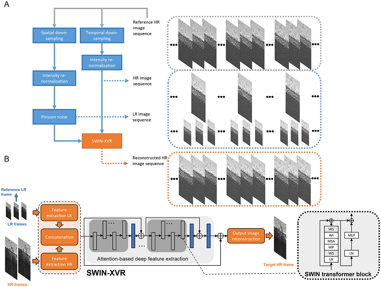
Figure 1. Illustration of (A) the spatio-temporal fusion numerical experiment workflow and (B) the architecture of the proposed model to reconstruct HR image sequences based on the SWIN vision transformer. The model inputs are consecutive LR and HR images that can be acquired from the corresponding UHS and HS cameras. The model output is configured as a single HR image at the time when the reference LR image is acquired.

3.2 Model architecture and training

As shown in Figure 1B, our model consists of three distinct modules, namely, the input feature extraction module, the attention-based deep feature enhancement module, and the output image reconstruction module, respectively. The input feature extraction module transforms the multi-resolution input images into shallow features. It consists of one branch to extract features from the input LR images and another one to extract features from the input HR images. The convolution outputs are directly used as the tokens (i.e., the tokenization patch size is 1 × 1) in the subsequent SWIN transformer module for deep feature enhancement. Instead of the convolutional spatio-temporal feature fusion module from Wang et al. (2019) and Tang et al. (2025), we extend the framework of image restoration using the Shifted Window (SWIN) transformer (Liang et al., 2021) to model the correlation among tokens from local spatio-temporal windows (Liu et al., 2022). Compared with the feature fusion model in Wang et al. (2019) and Tang et al. (2025), SWIN transformers provide additional scalability to the problem size. The attention-based deep feature enhancement module models and utilizes local correspondences among deep feature maps (Zeng et al., 2020) to enhance the feature maps of the target frame. More specifically, it consists of two hierarchies to propagate features across different time points and spatial scales.

At the bottom level of this hierarchy is the multi-head self-attention (MSA) layer and feed-forward network (FFN), to be referred to as a “SWIN transformer block” in the remainder of this paper. The MSA aims to jointly attend to multiple feature subspaces and aggregate features within each spatio-temporal window, i.e., within each local spatial window and from all feature maps. The two-layer FFN is cascaded with the MSA for feature fine adjustment. Prior to each MSA and FFN, layer normalization is performed to regularize the features generated throughout the deep network. Within each MSA layer and each feature subspace, a learnable relative position bias (RPB) is added to the self-attention maps computed from all local spatio-temporal windows to better model the spatial relationships among features (Hu et al., 2019). Next, several SWIN transformer blocks are stacked and grouped into multiple stages to allow the feature enhancement module to scale up according to the complexity of the task. Following each MSA and FFN, stochastic depth (Huang et al., 2016) is applied to randomly drop out samples within each training batch for better regularization and training performances. Window shift is applied alternately to the SWIN transformer blocks to expand the effective receptive field. Residual connection is further added between subsequent transformer stages to enhance feature propagation across different SWIN transformer stages. The output image reconstruction module then selects the target feature map from the collection of enhanced deep feature maps and upscales the spatial dimensions by a factor of 4 with the pixel shuffle up-sampling layers (Lim et al., 2017).

Training data consist of 1,358 videos recorded with a Photron FastCam SA-Z camera (Photron Inc., Japan) and a Shimadzu HPV-X2 camera (Shimadzu corporation, Japan) with frame rates 1–140 KHz and 1–5 MHz, respectively, covering a wide range of advanced manufacturing processes, during multiple high-speed synchrotron x-ray imaging experiments performed at the 32-ID beamline of the APS. Videos recorded with the Photron camera contain 101–8,901 frames and videos recorded with the Shimadzu camera contain 128 frames. For each video recorded with the Shimadzu camera, the first frame was not included for model training.

Low-resolution images were created by binning the high-resolution images with a 4 × 4 window (Peters et al., 2015). Four videos each containing 500 frames with 400 × 1,024 pixels per frame, were randomly sampled from all the videos and held out as validation data and the remaining were used as the training data. For the training data, random crops of 96 × 96 and 24 × 24 pixels were made on the corresponding HR and LR images to cover a spatially consistent region in each frame. Details of the data augmentation can be found in our previous work (Tang et al., 2025). The model was then trained to minimize the L1 loss, defined as:

$\begin{array}{ll}l(x,y)=\frac{1}{N}{\displaystyle \sum _{n=1}^N}|x_n-y_n|,& (1)\end{array}$

where x_n, y_n are the model output and ground-truth corresponding to the n-th sample in a batch (with a total of N samples), for a fixed number of iterations with the Adam optimizer and an initial learning rate of 0.0002. The learning rate was updated following the cosine annealing scheduler, with a small number of iterations in the beginning of training used for warmup (i.e., the initial learning rate was additionally scaled by the fractional iteration number in this warmup window). The drop rate in the stochastic depth was scaled uniformly to a maximum of 0.2.

Model training was performed using the PyTorch framework on the Polaris HPC system at the ALCF. Data parallelization was implemented by initiating multiple processes across 4 Nvidia A-100 SXM4 GPUs (40GB memory each) on a single computing node and also across multiple nodes. During training, one distinct GPU was selected for a process and all processes were synchronized at the end of each training iteration using the distributed data parallelization (DDP) library of PyTorch. The Nvidia collective communications library (NCCL) and the message passing interface (MPI) were used to communicate all GPU devices across multiple nodes. Model inference was performed on 4 Nvidia A100 SXM4 GPUs (40 GB memory each). For each video in the testing data, the reconstruction of the entire HR image sequence was equally distributed to 4 processes, with each process utilizing one GPU.

4 Experimental evaluation

Training experiments aim to characterize the model performance as a function of the computing environment and the model hyperparameters. More specifically, in this study, we investigated the model performance in terms of (1) its scaling capability when the number of GPUs in the data-parallelized training increases, and (2) the fidelity of the target HR image reconstruction when its spatio-temporal window size, the amount of training data, and the model size and architecture varied. The model scaling effect was benchmarked on the wall time of the model training algorithm running on a fixed number of training images distributed to a varying number of GPUs increasing from 4 to 256 by powers of 2. In addition, the scaling efficiency (Sarma et al., 2024) was also used to quantify the ability of the training job to utilize increased GPU resources, as defined below:

$\begin{array}{ll}e(r,g)=\frac{s(r,g)}{s^{*}(r,g)}\times 100\%,& (2)\end{array}$

where

$\begin{array}{ll}s(r,g)=\frac{{\bar{t}}_e(r)}{{\bar{t}}_e^{*}(g)},& (3)\end{array}$

${\bar{t}}_e(r)$ is the reference standard of training time with r GPUs, ${\bar{t}}_e^{*}(g)$ is the actual training time with g GPUs, and s^*(r, g) is the ideal speed up when the number of GPUs increases from r to g. The reconstruction fidelity was measured as the PSNR between the reconstructed HR image and the corresponding ground truth averaged from 4 independent x-ray image sequences (500 LR/HR frame pairs, with the model input consisting of a chunk of LR images of the prescribed frame number and another two HR images from the same times of the LR images immediately before and after the target image) after the model had been trained for a fixed number of iterations and convergence was confirmed. Formally, the average PSNR is defined as:

$\begin{array}{ll}{\overline{PSNR}}_{val}=\frac{1}{4}{\Sigma }_{j=1}^4{\overline{PSNR}}_j,& (4)\end{array}$

where

$\begin{array}{ll}{\overline{PSNR}}_j=\frac{1}{500}{\Sigma }_{i=1}^{500}{\overline{PSNR}}_{ij},& (5)\end{array}$

and ${\overline{PSNR}}_{ij}$ is the PSNR of the ith image from the jth video. The baseline model consisted of 24 SWIN transformer blocks grouped into 4 stages (each with 2, 2, 18, and 2 blocks, respectively), used 3 input LR images and 2 input HR images with the transformer blocks operating, via 3 concurrent attention heads, at spatial windows of size 8 × 8 and with tokens of 192 channels. For the spatio-temporal window, the number of LR frames was varied among 3, 5, 7, and 9 (in addition to another 2 HR frames), and the spatial window size was varied among 1 × 1, 2 × 2, 4 × 4, and 8 × 8. The initial training data set was randomly under-sampled to 0.07%, 0.1%, 0.5%, 1%, 10%, 40%, 70%, and 100% (i.e., no under-sampling) of its original size to train the model. To explore the influence of the model size on its performance, the following conditions were explored on top of the baseline setting.

1. The number of attention heads was reduced to 1,

2. The number of token channels was increased to 384,

3. The number of token channels was increased to 384, and the number of attention heads was increased to 6, and

4. The number of SWIN transformer blocks was increased to 48.

Model testing aims to evaluate the utility of the selected model on real-world applications. To achieve this, the optimal model hyperparameters were determined based on the validation results, and the selected model was trained for more iterations. Two independent x-ray videos for applications of additive manufacturing (Ren et al., 2023) and friction stir welding (Agiwal et al., 2022) were used to test the performance of the proposed image reconstruction algorithm. These two datasets have been previously uploaded to the tomobank repository (De Carlo et al., 2018) where meta data such as the sampling rate, number of frames, and number of pixels were made available¹. By applying a re-simulation technique similar to Tang et al. (2025), also briefly reviewed in Figure 1A, the original HR image frame separation was varied among 2, 10, 20, and 450, and the blank scan factor b₀ in the input LR images was varied to result in PSNRs of approximately 20 dB to 60 dB (in increments of 10 dB) plus infinity (corresponding to no Poisson noise simulated). The LR image frame separation was fixed at 1. These conditions were used to cover general settings of a high-speed imaging experiment and demonstrate method viability. The same performance metrics as in Tang et al. (2025), i.e., PSNR, average absolute difference (AAD), and structural similarity (SSIM), along with the corresponding wall time to reconstruct each single HR image were used to quantify the fidelity and efficiency of the HR image reconstruction.

5 Results

In this section, we report the performance of the proposed SWIN-XVR model at training time and at inference time to reconstruct HR x-ray videos. By leveraging the Polaris HPC system as the platform to train deep learning models, we first present a strong scalability analysis to characterize the wall time of a fixed training job when it is run by an increasing number of GPUs and with other appropriate hardware configurations. We then extend the training jobs to study a number of model parameters that are relevant to the runtime performance and scientific impact of the proposed algorithm when the model is trained and deployed on a typical operating environment in the high-speed imaging community. With the validated model parameters and training configurations, we scale up the model training, apply the trained model to the two testing datasets, and compare the resulting HR x-ray video reconstruction accuracy with that of another four independent algorithms, namely, the bicubic interpolation, Bayesian fusion (Xue et al., 2017), EDVR (Wang et al., 2019) and EDVR-STF (Tang et al., 2025), the latter two based on convolution-based deep neural network architecture.

Figure 2 illustrates the influence of the training batch size on two types of the GPU times, namely, the idle time and the non-idle time, and the GPU utilization. Overall, the idle time decreases consistently as the batch size increases from 1 to 5 and plateaus for larger batch sizes (e.g., 5, 10, and 20). For the non-idle time, it shows an increasing trend when the batch size increases. As a result, the GPU utilization increases with the batch size and exceeds 90% with more than 5 samples in a batch. In the remainder of the scalability analysis, the batch size will be fixed at 10.

Figure 2

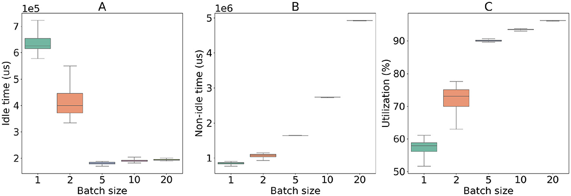
Figure 2. Illustration of the GPU time composition as the idle time (A), non-idle time (B), and the GPU utilization (C) each as a function of the underlying training sample batch size. At each specific batch size, the distributed training experiment was performed with 40 GPU devices for a fixed period of 10 consecutive iterations. The GPU time performance was profiled using the Pytorch profiler package and analyzed using the holistic trace analysis (HTA) package.

Figure 3 illustrates the scalability of the model training to the number of GPUs allocated. To demonstrate the strong scaling efficiency, the total number of images was fixed at 1,206,240 (upsampled from the original dataset with data augmentation). In Figures 3A, B, it is clear that with the specific size of training data, the job converges at iteration 30,000 with 4 GPUs utilized. According to Figure 3C, overall, the wall time decreases with an increasing number of GPUs. As the total training data were equally divided to be used by each GPU device, an increase in the number of GPUs effectively reduced the initial problem size, leading to shorter wall times. The computation results also indicate that, as the number of GPUs increases, the wall time eventually converges to a positive value (hence the deflection of the actual wall times from the fitting line toward the positive side), which may be attributed to the communication among GPUs during the distributed training. Figure 3D confirms that when up to 32 GPUs are utilized for the training job, good scalability (above 90%) is observed. Utilizing more than 32 GPUs for the training job starts to reduce the scaling efficiency.

Figure 3

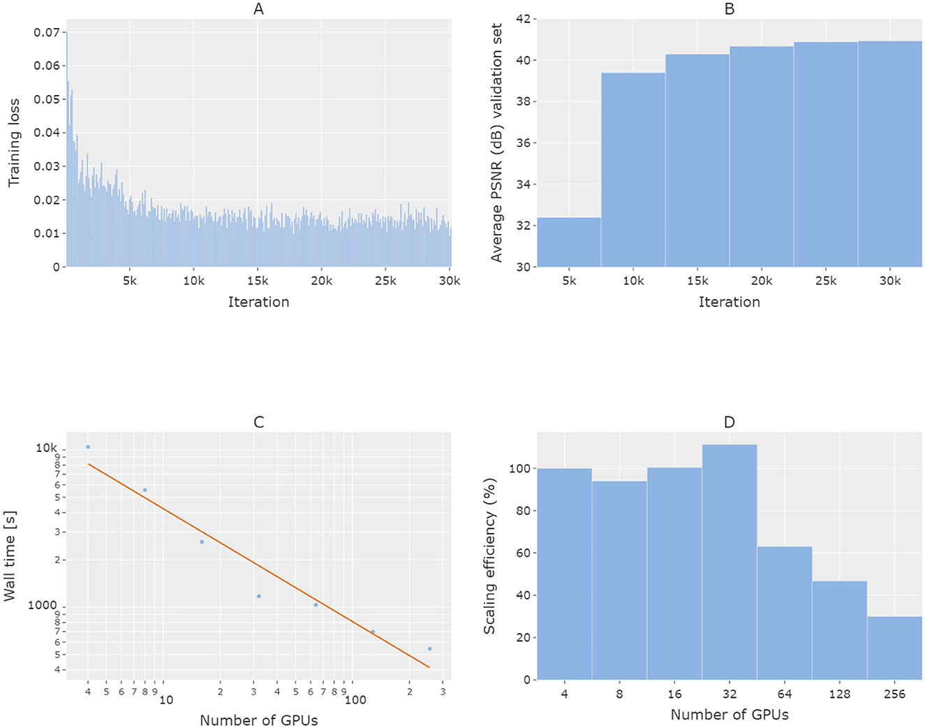
Figure 3. Illustration of the distributed training strong scalability analysis. (A) Training loss and (B) validation accuracy over the number of training iterations at baseline with 4 GPUs. (C, D) Wall time and scaling efficiency of the end-to-end training jobs over the number of GPUs utilized in each job. Validation in (B) was performed once after every 5,000 training iterations. Both the x- and y- axes in (C) are in the log space (base-10) and the x-axis in (D) is in the log space (base-2). The solid curve in (C) indicates a linear fit in the log-log space (base-10) of the type log₁₀(y) = b + alog₁₀(x), where a = −0.72 and b = 4.34.

Figure 4 further shows the distributions of different kernel times when the training jobs were executed with varying numbers of GPUs. More specifically, the communication kernels denote those intended for the NCCL-enabled algorithms such as the AllReduce algorithms with various topologies and the broadcast algorithm, in addition to the copy operations between the host and device memories. Whereas the computation and memory kernels denote those used for tensor operations, and initialization/copy operations within the device memory, respectively. For a given number of GPUs allocated to the distributed training, the computation, communication, and memory kernel times were averaged across all the GPU devices and organized in a pie chart to showcase their relative contributions to the total kernel time. According to the results, the percentage of the computation kernel time generally decreases with the number of GPUs, with the opposite trend visible in the percentage of the communication kernel time. The percentage of the memory kernel time remains approximately constant.

Figure 4

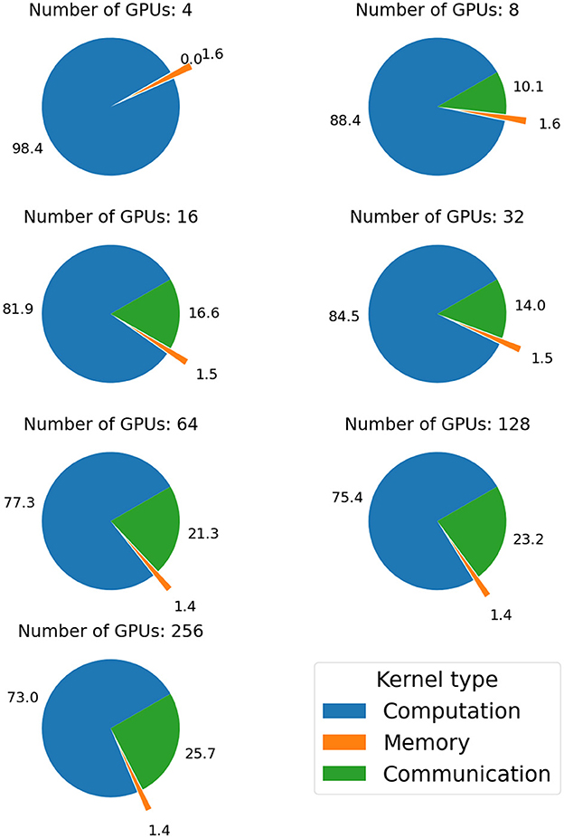
Figure 4. Illustration of the GPU's kernel time due to computation, communication, and memory operations and their changes with the number of GPUs utilized in the distributed training. A fixed number of 3 iterations were concentrated on to profile and analyze the kernel times.

Figure 5 shows the accuracy of the model for various training configurations on the validation dataset. Given each configuration, the model was trained for 30,000 iterations (warmup applied to the first 500 iterations) with the highest PSNR reported. In Figure 5A, the effect of different number of input LR frames on the reconstructed HR image PSNR is investigated. According to the results, no clear trend is observed, which is also consistent with the two testing datasets (Supplementary Figures S1A, S2A). In Supplementary Figures S3, S4, the number of input LR frames are further analyzed using the testing data with the input LR images subjected to various degrees of Poisson noise, and both when the input HR frames are close (i.e., with a frame separation of 2) and are temporally distant (i.e., with a frame separation of 20). When the HR frames are close, no significant improvement is observed in increasing the number of input LR frames at each given input LR image PSNR. When the HR frames are distant, increasing the number of input LR frames shows a slight improvement in all 3 performance metrics, consistently with the two cases and across all input LR image PNSR levels. Figure 5B shows the same PSNR metrics with varying window sizes configured for the SWIN transformer blocks (results on the two testing datasets are presented in Supplementary Figures S1B, S2B). Compared with the baseline setting of an 8 × 8 attention window, the choice of smaller window sizes appears more plausible. In Figure 5C, the training data are reduced to different fractions of its original size to train the baseline model. As can be seen from the results, there is an overall monotonic increasing pattern in the resulting PSNR when the training dataset grows in size. In addition, the PSNR increase becomes less pronounced when the model is trained on the subset of the training data of larger than 0.5%–1% of its original size. When the same models are applied to the testing data, similar trends can be observed from both datasets (Supplementary Figures S1C, S2C). In comparison, the welding dataset shows a relatively lower sensitivity to the training data size. Last, Figure 5D compares the model performances when incremental changes in its size and architecture are introduced. More specifically, compared to the baseline model, a decrease in the number of attention heads to 1 in the transformer block results in a slight decrease in the PSNR, doubling the model depth results in a slight increase in the PSNR, and doubling the hidden size (token channel number) significantly improves the PSNR, consistently with the validation data and testing data (Supplementary Figures S1D, S2D). Compared to the configuration with doubling the hidden size, further doubling the number of attention heads (to 6) leads to inconsistent changes in the PSNR across the validation and testing datasets.

Figure 5

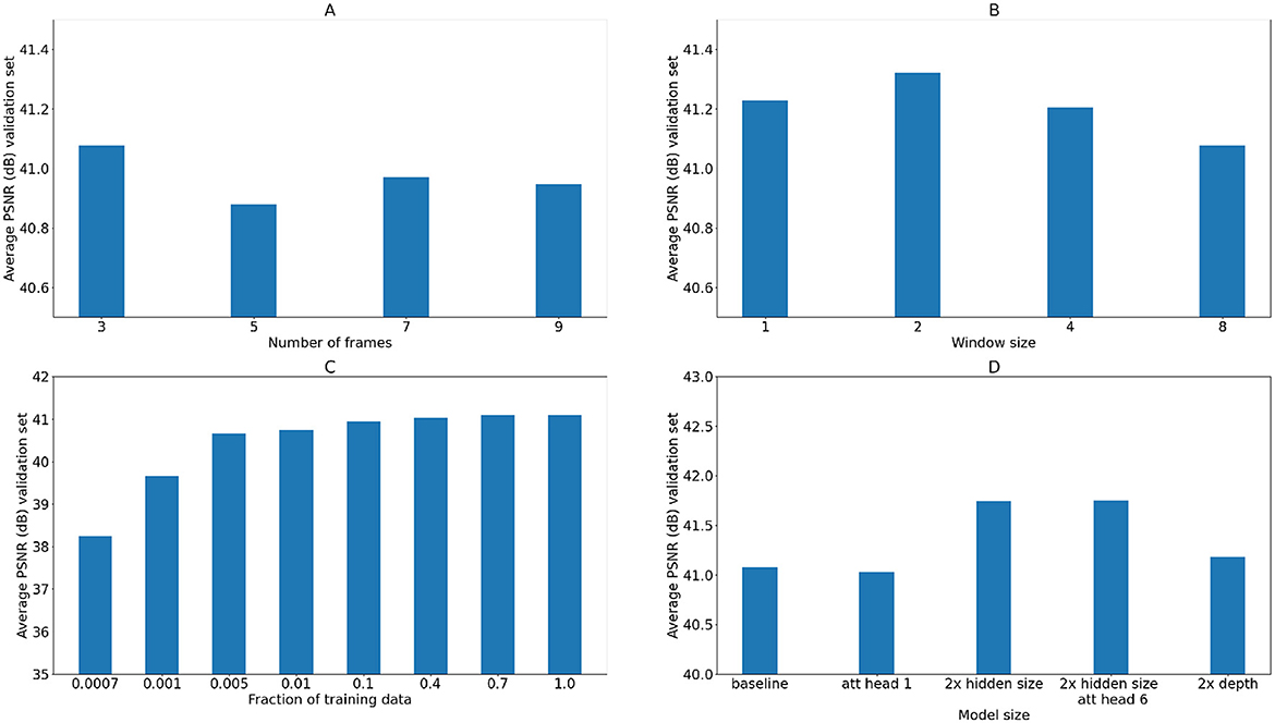
Figure 5. Average PSNR (dB) on the validation dataset as a function of the number of input LR frames (A), the attention head spatial window size (B), the number of videos used for training relative to the total number of training videos (C), and the model size and architecture parameters (D).

When each model as compared in Figure 5 is applied to the two testing datasets, the corresponding wall time averaged over each reconstructed HR image sequence is reported in Figure 6. In particular, the wall time shows an increasing trend along with both the increasing number of frames (Figure 6A) and increasing window size (Figure 6B), consistently with both datasets. Increasing the number of attention heads slightly increases the wall time also. Last, the wall time shows a significant increase with either double the hidden channels or double the model depth, by a factor of 2.15 and 1.93 in case 1 and 2.18 and 1.94 in case 2. Based on the results from Figures 5, 6, the number of input LR frames of the model was determined to be 3, with a window size 4 × 4, hidden size of the token embedding 384, and 6 attention heads in each transformer block to balance the accuracy and inference speed.

Figure 6

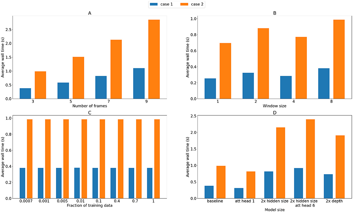
Figure 6. Inference wall time of the testing dataset as a function of the number of input LR frames (A), the attention head spatial window size (B), the number of videos used for training relative to the total number of training videos (C), and the model size and architecture parameters (D).

With the validated model hyperparameters, the model was trained for 75,000 iterations (warmup applied to the first 2,000 iterations). Figure 7 compares selected reconstructed HR images (column C) with the corresponding LR (column A) and HR (column B) images qualitatively for both the additive manufacturing (row 1) and friction stir welding (row 2) applications. Fine-scale spatial details in both cases are demonstrated to be restored with great clarity. Figure 8 compares the PSNR, AAD, and SSIM of bicubic interpolation, Bayesian fusion, EDVR, EDVR-STF, and SWIN-XVR on the 2 testing datasets with varying LR image PSNRs due to Poisson noise. Overall, all 3 metrics improve with higher PSNR in the input LR images, consistent with the two testing datasets. When the 5 algorithms are compared, performance of SWIN-XVR is close to and significantly better than that of EDVR-STF on cases 1 and 2, respectively. With lower PSNR in the input LR images, the performance in terms of PSNR and AAD of SWIN-XVR drops slightly faster than EDVR-STF (while drops in SSIM remain similar). With reduced noise in the LR images (i.e., LR image PSNR 50 dB or above), the Bayesian fusion starts to demonstrate higher accuracy (i.e., the maximum PSNR and SSIM, and the minimum AAD) than other methods in the reconstructed HR images for case 1, in the absence of the underlying scene motion. However, in general, its performance in the presence of complex motion dynamics drops significantly. The deep learning-based algorithms consistently outperforms the bicubic interpolation. Figure 9 compares the same with varying down-sampling factors to temporally down-sample the HR image sequence and with the original frame separation of the LR image sequence. SWIN-XVR and EDVR-STF both show an overall performance drop in terms of the 3 performance metrics with larger separations in the input HR images (bicubic interpolation and EDVR are not affected as they do not rely on any HR images). Similar to the trend in Figure 8, the performance of SWIN-XVR is close to and mostly no better than EDVR-STF on case 1, whereas it significantly outperforms the latter on case 2. SWIN-XVR again shows additional performance drops with increasing HR frame separations compared with its EDVR-STF counterpart, most prominently when only the first and last HR frames in the entire image sequence is used to reconstruct the intermediate frames. In such a situation, the median PSNR of SWIN-XVR is lower and the median AAD of SWIN-XVR is larger than those of EDVR for case 2. Bayesian fusion is not evaluated because the testing condition violates its configuration. The deep learning-based algorithms perform generally better than the bicubic interpolation, with the exception of on case 2 when the HR frames are temporally down-sampled by a factor of 450. In such a situation, the median AAD of SWIN-XVR is smaller than that of the bicubic interpolation, but the peak AAD is larger than that of bicubic interpolation. Details in the configurations of the selected baseline methods can be found in Tang et al. (2025).

Figure 7

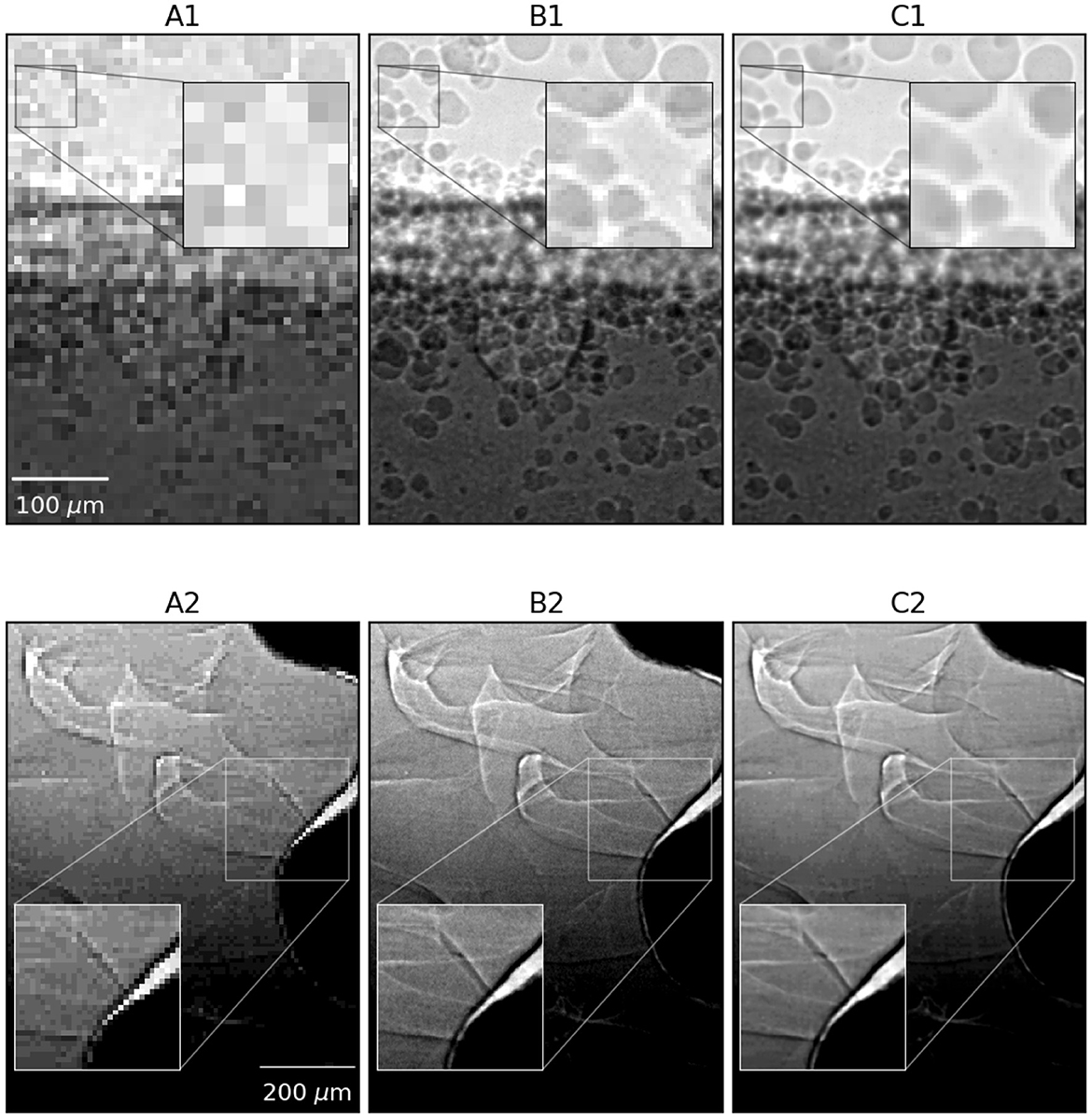
Figure 7. Selected LR images of 4 times larger pixel size (column A), HR images of 20 times larger frame separation (column B), reconstructed HR images (column C) for applications of additive manufacturing (row 1) and friction stir welding (row 2), respectively.

Figure 8

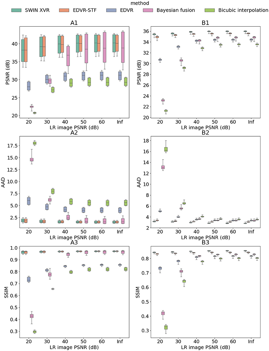
Figure 8. Reconstructed HR frame PSNR (dB) (row 1), AAD (row 2), and SSIM (row 3) each as a function of the LR image PSNR that was used to generate the Poisson noise in the input LR frames, based on bicubic interpolation, Bayesian fusion, EDVR, EDVR-STF, and SWIN-XVR. Results were evaluated on case 1 (column A) and case 2 (column B) and presented as box plots. Under each testing condition, the same samples as used for SWIN-XVR were used to test all other 4 algorithms.

Figure 9

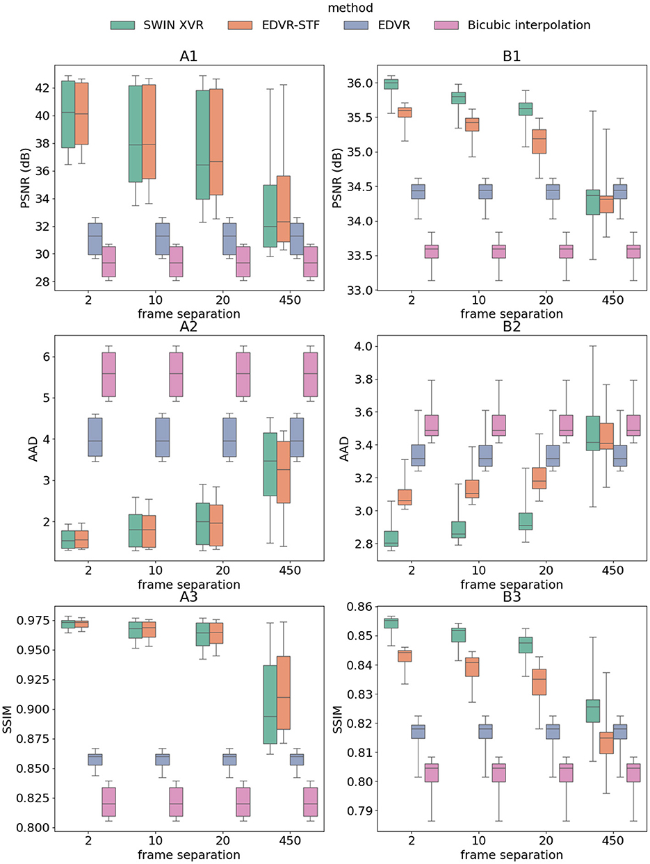
Figure 9. Reconstructed HR frame PSNR (dB) (row 1), AAD (row 2), and SSIM (row 3) each as a function of the HR frame sequence down-sampling factor, based on bicubic interpolation, EDVR, EDVR-STF, and SWIN-XVR. Results were evaluated on case 1 (column A) and case 2 (column B) and presented as box plots. LR separation was 1 across all plots. Under each testing condition, the same samples as used for SWIN-XVR were used to test all other 3 algorithms. No Poisson noise was generated for the testing data.

6 Discussion

In this paper, we present a full computation pipeline for a vision transformer (ViT)-based deep learning model, termed the “SWIN-XVR” to reconstruct high resolution and high frame rate x-ray videos with high fidelity that can be utilized by the synchrotron radiation facilities. For one thing, compared to the CNN which has been well studied for various computer vision applications, the use of ViT in similar applications is still nascent. For the specific problem of spatio-temporal video fusion, no existing ViT-based models can be directly applied. As a result, a comprehensive analysis of the hyperparameters of the SWIN-XVR model can provide useful information on the optimal model configuration and its implications to an actual x-ray imaging experiment to establish it as a new benchmark solution. For another, training of the SWIN-XVR model using the HPC resources can effectively emulate the realistic workflow of new model development, which can be reproduced in prospective development efforts. Powered by the distributed computing capability of the Polaris HPC system at the ALCF, model training and hyperparameter tuning can be performed with an efficiency several orders higher than a single-GPU system to allow rapid development of deep learning algorithms. This computation pipeline is intended to be reproducible during the routine operations of a UHS imaging beamline, such as the 32-ID at the APS.

The deployment of a dual camera-based optical assembly and the image reconstruction software at the beamline can significantly increase the scientific value of the HS experiments. In addition, because the UHS and HS cameras are configured to operate in parallel, the user experience will also be improved by avoiding frequent switching of cameras, which could take a prohibitive amount of time during the experiments. Currently, the total average experiment duration (set-up, acquisition, and sample change) is in the range of ~10 min to 1 h, and the use of the proposed image acquisition/reconstruction framework will thus double the data throughput within the same time budget. With techniques such as domain adaptation (Ganin et al., 2016), the proposed method could be further generalized to image sequences generated by other detectors or other modalities, such as computerized tomography (CT) (Wu et al., 2020; Liu et al., 2020) and magnetic resonance imaging (MRI) (Georgescu et al., 2023) to perform similar tasks at other beamlines and, in general, in other application domains. The algorithm is implemented in Python and publicly available at https://github.com/xray-imaging/XFusion. Currently, the algorithm takes about 115 seconds to finish the reconstruction of 500 HR images of dimension 400 × 1,024 with 4 Nvidia A-100 SXM4 GPUs. In the future, imaging data accumulated at the beamline could be transferred to the HPC systems to train highly performant deep learning models at scale employing a foundational training approach (Ma et al., 2024). These foundation models can generalize to unseen novel imaging data with exceptional generalizability, and can be deployed back to the local application servers at the beamlines and fine-tuned to perform specific tasks, support the ongoing user services with improved accuracy, automation, and robustness, and offer extended scientific value.

During the execution of training jobs of deep learning models, the GPU utilization and the wall time are two critical indices to characterize the computation performance. To characterize the GPU utilization, the compute usage, i.e., the percentage of time a GPU spends running a kernel (as compared to staying idle) was considered in this study and monitored when the underlying batch size of the training samples was increased. More specifically, with the aid of the HTA software package, we monitored the starting time and the time duration associated with each GPU kernel when it was active during a fixed time period of 10 training iterations. We then computed the non-idle time as the total time duration when at least one GPU kernel was active and the idle time as the complement to the non-idle time in the monitoring period. The GPU utilization was then derived as the percentage of the non-idle time in the same period. According to the results, there was a positive correlation between the batch size and the GPU utilization, confirming the role of larger batches in improving parallelism of model training. We then fixed the batch size at 10 (corresponding to a GPU utilization of more than 93%) to train the baseline SWIN-XVR model with the same amount of data for repeated times, differing in the number of GPUs each time to characterize the strong scaling effect. The results on the scaling efficiency reveals a trend in the wall time with the number of GPUs that roughly follows an inverse proportional curve (a line in the log-log space) especially when the number of GPUs utilized is below 32. This in turn indicates a good scaling performance of the Polaris system within the number of GPUs of choice, i.e., the wall time is commensurate to the time to effectively update the model weights for up to 32 GPUs. Whereas utilizing more GPUs (32 to 256) starts to show decrease in the scaling efficiency given our specific training configuration. Due to the relatively small problem size, we did not further investigate the scaling effect with more GPUs. Repeating the same GPU configurations as in the scalability analysis for extra training experiments each with a fixed time period of 3 training iterations, we also compared the participation of different types of GPU kernels. The increasing duration of the communication kernels reflects the increasing overhead of the training jobs. As a result, the training time will face a lower bound as the number of GPUs continues to increase. In addition, upscaling the training jobs in practice also needs to consider model accuracy along with the increasing number of GPUs. With the specific job size to study training scaliability, we observed good convergence when 4 GPUs were used. More training data/iterations may be required to keep up with the target model accuracy when a larger number of GPUs is utilized.

When the model hyperparameters were validated, we studied the effect of the number of input LR frames, the size of the spatial window for the local attention operations, the fraction of the total training data, and variations in the model architecture and size. From a computation point of view, a smaller number of input LR frames leads to faster HR image reconstructions during the high-speed imaging experiments. According to the results, the choice of 3 input LR frames not only results in a shorter inference time, but also maintains a comparable accuracy in the reconstructions among various configurations. In terms of the window size, in the light of Liu Z. et al. (2021), it is positively correlated with the computational complexity, hence the reconstruction time. As the results suggest, the choice of a size of 4 × 4 provides a plausible trade-off between the computation complexity and reconstruction errors. As for the fraction of the training data, it is meant to provide recommendations for prospective efforts on the training dataset construction. Since the nature of a high-speed imaging experiment is invariably diversity-starved, i.e., under each type of experiments, the same imaging parameters could be repeated for multiple times, a small amount of training videos of distinct types would suffice to yield an accurate model for the spatio-temporal fusion task. From the results, we observed the performance growth to gradually slow down when the dataset was more than 0.5%–1% of its original size. This would imply that the desired training dataset only requires a very marginal amount of additional acquisitions during each new experiment. Last, among different model architectures and sizes, the model with 2 times of the hidden dimension results in a significant improvement (up to 0.8 dB for case 1) in the reconstruction error at the necessary cost on the inference time that scales up proportionally. While doubling the number of attention heads to 6 adds only a moderate computation cost (12.10% for case 1 and 11.30% for case 2) for extra flexibility in modeling more complex spatio-temporal dynamics in the data. With 2 times of the model depth, the inference time increases by a similar factor, but with only a slight improvement (up to 0.12 dB for case 1) in the reconstruction accuracy. As a result, we doubled the model hidden size and used 6 attention heads for the final model architecture.

Two testing conditions were created to evaluate the model as applied to a real high-speed imaging experiment to monitor different physical phenomena in operando. Among them, the variation in the input LR image PSNR was used to emulate changes in the shutter speed of a UHS camera, and the HR image sequence was assumed to be in a noise-free condition. On the other hand, the variation in the HR image sequence down-sampling rate was used to cover scenarios where the temporal dynamics of the physical phenomena was under-sampled to different extents, which can happen in practice as the underlying dynamics often manifest at distinct time scales. These testing conditions have been used in our previous paper to evaluate the convolution-based model (Tang et al., 2025). Overall, the SWIN-XVR model demonstrated a comparable performance to the EDVR-STF with an improved generalization capability, except for extreme conditions in the HR frame separation. In Supplementary Figures S3, S4, when the number of the input LR frames was increased, we observed a slight improvement in the reconstruction quality under different noise conditions in the input LR images only when there was a large separation (e.g., 20 frames) in the input HR images. When the HR frames are distant, their correlations with the time of the target frame decrease, and the importance of the LR frames in the reconstruction could in turn increase. In such a situation, a larger number of LR frames may help aggregate more information about the underlying physical process at the target time point and reduce the uncertainty due to noise, particularly in spatial regions with relatively insignificant motion. However, as the number of LR frames continues to increase, the complexity in the spatio-temporal distribution of coherent features also increases, which could confound the denoising effect in the accuracy metrics. In the future, more dedicated studies will be performed to verify this effect, with authentic image sequences from the HS and UHS cameras.

7 Conclusions and outlook

In this paper, we present the use of the HPC system for the training and validation of a SWIN-based vision transformer (ViT), called the “SWIN-XVR” to fuse spatial and temporal sub-samples of image sequences acquired from a high-speed x-ray imaging experiment. We utilized the Polaris HPC system located at the ALCF and the PyTorch DDP framework to scale up the model training to multiple GPUs and multiple computing nodes and for a wide range of hyper-parameters of interest. Such an algorithmic framework allowed rapid experimentation with candidate deep learning-based models to establish new benchmarks. The validated model was applied to two testing datasets from typical high-speed imaging experiments and demonstrated high accuracy compared to past methods. In the future, this presented work can be instrumental to the construction of an efficient processing pipeline at the synchrotron radiation facility, such as the APS to optimize the planning of the lifecycle of the massive imaging data generated during its routine operations.

Data availability statement

The data analyzed in this study is subject to the following licenses/restrictions: this product includes software/data produced by UChicago Argonne, LLC under Contract No. DE-AC02-06CH11357 with the Department of Energy. It is provided for use subject to the disclaimer below. Redistribution and use with or without modification are permitted. Please include this notice and credit Argonne National Laboratory if you use or distribute it further. Disclaimer the software/data is supplied “as is” without warranty of any kind. Neither the United States Government, nor the United States Department of Energy, nor UChicago Argonne, LLC, nor any of their employees, makes any warranty, express or implied, or assumes any legal liability or responsibility for the accuracy, completeness, or usefulness of any information, data, apparatus, product, or process disclosed, or represents that its use would not infringe privately owned rights. Requests to access these datasets should be directed to https://tomobank.readthedocs.io/en/latest/source/data/docs.data.radio.html#xradfusion.

Author contributions

ST: Conceptualization, Data curation, Formal analysis, Investigation, Methodology, Software, Validation, Visualization, Writing – original draft, Writing – review & editing. TB: Conceptualization, Funding acquisition, Resources, Writing – original draft, Writing – review & editing. KF: Conceptualization, Funding acquisition, Resources, Writing – original draft, Writing – review & editing. SC: Conceptualization, Funding acquisition, Project administration, Resources, Writing – original draft, Writing – review & editing.

Funding

The author(s) declare that financial support was received for the research and/or publication of this article. This research used resources of the Advanced Photon Source, a U.S. Department of Energy (DOE) Office of Science user facility and is based on work supported by Laboratory Directed Research and Development (LDRD) funding from Argonne National Laboratory, provided by the Director, Office of Science, of the U.S. DOE under Contract No. DE-AC02-06CH11357. This research used resources of the Argonne Leadership Computing Facility, a U.S. Department of Energy (DOE) Office of Science user facility at Argonne National Laboratory and is based on research supported by the U.S. DOE Office of Science, Advanced Scientific Computing Research Program, under Contract No. DE-AC02-06CH11357.

Acknowledgments

The authors acknowledge Dr. Tao Sun (Northwestern University), Dr. Frank E. Pfefferkorn (University of Wisconsin-Madison), Dr. Yunhui Chen (RMIT University), and Dr. Atieh Moridi (Cornell University) for allowing the use of the x-ray datasets for model training and testing.

Conflict of interest

The authors declare that the research was conducted in the absence of any commercial or financial relationships that could be construed as a potential conflict of interest.

The author(s) declared that they were an editorial board member of Frontiers, at the time of submission. This had no impact on the peer review process and the final decision.

Generative AI statement

The author(s) declare that no Gen AI was used in the creation of this manuscript.

Publisher's note

All claims expressed in this article are solely those of the authors and do not necessarily represent those of their affiliated organizations, or those of the publisher, the editors and the reviewers. Any product that may be evaluated in this article, or claim that may be made by its manufacturer, is not guaranteed or endorsed by the publisher.

Supplementary material

The Supplementary Material for this article can be found online at: https://www.frontiersin.org/articles/10.3389/fhpcp.2025.1537080/full#supplementary-material

Footnotes

1. ^https://tomobank.readthedocs.io/en/latest/source/data/docs.data.radio.html#xradfusion

References

Agiwal, H., Ansari, M. A., Franke, D., Faue, P., Clark, S. J., Fezzaa, K., et al. (2022). Material flow visualization during friction stir welding using high-speed x-ray imaging. Manufact. Lett. 34, 62–66. doi: 10.1016/j.mfglet.2022.08.016

Crossref Full Text | Google Scholar

Benmore, C., Bicer, T., Chan, M. K., Di, Z., Gürsoy, D., Hwang, I., et al. (2022). Advancing AI/ML at the advanced photon source. Synchrotron Radiat. News 35, 28–35. doi: 10.1080/08940886.2022.2112500

Crossref Full Text | Google Scholar

Chen, L., Ye, M., Ji, L., Li, S., and Guo, H. (2024). Multi-reference-based cross-scale feature fusion for compressed video super resolution. IEEE Trans. Broadcast. 99, 1–44. doi: 10.1109/TBC.2024.3407517

Crossref Full Text | Google Scholar

Chen, Z., Zhang, Y., Gu, J., Kong, L., Yang, X., and Yu, F. (2023). “Dual aggregation transformer for image super-resolution,” in Proceedings of the IEEE/CVF International Conference on Computer Vision, 12312–12321. doi: 10.1109/ICCV51070.2023.01131

PubMed Abstract | Crossref Full Text | Google Scholar

De Carlo, F., Gürsoy, D., Ching, D. J., Batenburg, K. J., Ludwig, W., Mancini, L., et al. (2018). Tomobank: a tomographic data repository for computational x-ray science. Measur. Sci. Technol. 29:034004. doi: 10.1088/1361-6501/aa9c19

Crossref Full Text | Google Scholar

Dosovitskiy, A. (2020). An image is worth 16x16 words: transformers for image recognition at scale. arXiv preprint arXiv:2010.11929.

Google Scholar

Escauriza, E., Duarte, J., Chapman, D., Rutherford, M., Farbaniec, L., Jonsson, J., et al. (2020). Collapse dynamics of spherical cavities in a solid under shock loading. Sci. Rep. 10:8455. doi: 10.1038/s41598-020-64669-y

PubMed Abstract | Crossref Full Text | Google Scholar

Ganin, Y., Ustinova, E., Ajakan, H., Germain, P., Larochelle, H., Laviolette, F., et al. (2016). Domain-adversarial training of neural networks. J. Mach. Learn. Res. 17, 1–35.

Google Scholar

Gao, F., Masek, J., Schwaller, M., and Hall, F. (2006). On the blending of the landsat and modis surface reflectance: predicting daily landsat surface reflectance. IEEE Trans. Geosci. Rem. Sens. 44, 2207–2218. doi: 10.1109/TGRS.2006.872081

Crossref Full Text | Google Scholar

Georgescu, M.-I., Ionescu, R. T., Miron, A.-I., Savencu, O., Ristea, N.-C., Verga, N., et al. (2023). “Multimodal multi-head convolutional attention with various kernel sizes for medical image super-resolution,” in Proceedings of the IEEE/CVF Winter Conference on Applications of Computer Vision, 2195–2205. doi: 10.1109/WACV56688.2023.00223

Crossref Full Text | Google Scholar

Hong, D., Yao, J., Wu, X., Chanussot, J., and Zhu, X. (2020). “Spatial-spectral manifold embedding of hyperspectral data,” in The International Archives of the Photogrammetry, Remote Sensing and Spatial Information Sciences, XLIII-B3-2020, 423–428. doi: 10.5194/isprs-archives-XLIII-B3-2020-423-2020

Crossref Full Text | Google Scholar

Hu, H., Zhang, Z., Xie, Z., and Lin, S. (2019). “Local relation networks for image recognition,” in Proceedings of the IEEE/CVF International Conference on Computer Vision, 3464–3473. doi: 10.1109/ICCV.2019.00356

Crossref Full Text | Google Scholar

Huang, G., Sun, Y., Liu, Z., Sedra, D., and Weinberger, K. Q. (2016). “Deep networks with stochastic depth,” in Computer Vision-ECCV 2016: 14th European Conference, Amsterdam, The Netherlands, October 11–14, 2016, Proceedings, Part IV 14 (Springer), 646–661. doi: 10.1007/978-3-319-46493-0_39

Crossref Full Text | Google Scholar

Liang, J., Cao, J., Sun, G., Zhang, K., Van Gool, L., and Timofte, R. (2021). “SwinIR: image restoration using swin transformer,” in Proceedings of the IEEE/CVF International Conference on Computer Vision, 1833–1844. doi: 10.1109/ICCVW54120.2021.00210

Crossref Full Text | Google Scholar

Lim, B., Son, S., Kim, H., Nah, S., and Mu Lee, K. (2017). “Enhanced deep residual networks for single image super-resolution,” in Proceedings of the IEEE Conference on Computer Vision and Pattern Recognition Workshops, 136–144. doi: 10.1109/CVPRW.2017.151

Crossref Full Text | Google Scholar

Liu, R., Deng, H., Huang, Y., Shi, X., Lu, L., Sun, W., et al. (2021). “Fuseformer: fusing fine-grained information in transformers for video inpainting,” in Proceedings of the IEEE/CVF International Conference on Computer Vision, 14040–14049. doi: 10.1109/ICCV48922.2021.01378

Crossref Full Text | Google Scholar

Liu, Z., Bicer, T., Kettimuthu, R., and Foster, I. (2019). “Deep learning accelerated light source experiments,” in 2019 IEEE/ACM Third Workshop on Deep Learning on Supercomputers (DLS) (IEEE), 20–28. doi: 10.1109/DLS49591.2019.00008

Crossref Full Text | Google Scholar

Liu, Z., Bicer, T., Kettimuthu, R., Gursoy, D., De Carlo, F., and Foster, I. (2020). Tomogan: low-dose synchrotron x-ray tomography with generative adversarial networks: discussion. JOSA A 37, 422–434. doi: 10.1364/JOSAA.375595

PubMed Abstract | Crossref Full Text | Google Scholar

Liu, Z., Lin, Y., Cao, Y., Hu, H., Wei, Y., Zhang, Z., et al. (2021). “Swin transformer: hierarchical vision transformer using shifted windows,” in Proceedings of the IEEE/CVF International Conference on Computer Vision, 10012–10022. doi: 10.1109/ICCV48922.2021.00986

Crossref Full Text | Google Scholar

Liu, Z., Ning, J., Cao, Y., Wei, Y., Zhang, Z., Lin, S., et al. (2022). “Video swin transformer,” in Proceedings of the IEEE/CVF Conference on Computer Vision and Pattern Recognition, 3202–3211. doi: 10.1109/CVPR52688.2022.00320

Crossref Full Text | Google Scholar

Lu, M., Chen, T., Dai, Z., Wang, D., Ding, D., and Ma, Z. (2023). Decoder-side cross resolution synthesis for video compression enhancement. IEEE Trans. Multim. 25, 2097–2110. doi: 10.1109/TMM.2022.3142414

Crossref Full Text | Google Scholar

Luo, S., Jensen, B., Hooks, D., Fezzaa, K., Ramos, K., Yeager, J., et al. (2012). Gas gun shock experiments with single-pulse x-ray phase contrast imaging and diffraction at the advanced photon source. Rev. Sci. Instr. 83:073903. doi: 10.1063/1.4733704

PubMed Abstract | Crossref Full Text | Google Scholar

Ma, C., Tan, W., He, R., and Yan, B. (2024). Pretraining a foundation model for generalizable fluorescence microscopy-based image restoration. Nat. Methods 21, 1558–1567. doi: 10.1038/s41592-024-02244-3

PubMed Abstract | Crossref Full Text | Google Scholar

Manin, J., Skeen, S. A., and Pickett, L. M. (2018). Performance comparison of state-of-the-art high-speed video cameras for scientific applications. Opt. Eng. 57, 124105–124105. doi: 10.1117/1.OE.57.12.124105

Crossref Full Text | Google Scholar

Miyauchi, K., Takeda, T., Hanzawa, K., Tochigi, Y., Sakai, S., Kuroda, R., et al. (2014). “Pixel structure with 10 nsec fully charge transfer time for the 20m frame per second burst cmos image sensor,” in Image Sensors and Imaging Systems 2014 (SPIE), 15–26. doi: 10.1117/12.2042373

Crossref Full Text | Google Scholar

Parab, N. D., Zhao, C., Cunningham, R., Escano, L. I., Fezzaa, K., Everhart, W., et al. (2018). Ultrafast x-ray imaging of laser-metal additive manufacturing processes. J. Synchrotron Radiat. 25, 1467–1477. doi: 10.1107/S1600577518009554

PubMed Abstract | Crossref Full Text | Google Scholar

Peters, C. J., Danehy, P. M., Bathel, B. F., Jiang, N., Calvert, N., and Miles, R. B. (2015). “Precision of fleet velocimetry using high-speed cmos camera systems,” in 31st AIAA Aerodynamic Measurement Technology and Ground Testing Conference, 2565. doi: 10.2514/6.2015-2565

Crossref Full Text | Google Scholar

Ramos, K., Jensen, B., Iverson, A., Yeager, J., Carlson, C., Montgomery, D., et al. (2014). In situ investigation of the dynamic response of energetic materials using impulse at the advanced photon source. J. Phys. 500:142028. doi: 10.1088/1742-6596/500/14/142028

Crossref Full Text | Google Scholar

Ren, Z., Gao, L., Clark, S. J., Fezzaa, K., Shevchenko, P., Choi, A., et al. (2023). Machine learning-aided real-time detection of keyhole pore generation in laser powder bed fusion. Science 379, 89–94. doi: 10.1126/science.add4667

PubMed Abstract | Crossref Full Text | Google Scholar

Sarma, R., Inanc, E., Aach, M., and Lintermann, A. (2024). Parallel and scalable AI in HPC systems for CFD applications and beyond. Front. High Perform. Comput. 2:1444337. doi: 10.3389/fhpcp.2024.1444337

Crossref Full Text | Google Scholar

Tang, S., Bicer, T., Sun, T., Fezzaa, K., and Clark, S. J. (2025). Deep learning-based spatio-temporal fusion for high-fidelity ultra-high-speed x-ray radiography. Synchrotron Radiat. 32, 432–444. doi: 10.1107/S1600577525000323

PubMed Abstract | Crossref Full Text | Google Scholar

Vaswani, A. (2017). “Attention is all you need,” in Advances in Neural Information Processing Systems.

Google Scholar

Wang, X., Chan, K. C., Yu, K., Dong, C., and Change Loy, C. (2019). “EDVR: video restoration with enhanced deformable convolutional networks,” in Proceedings of the IEEE/CVF Conference on Computer Vision and Pattern Recognition Workshops. doi: 10.1109/CVPRW.2019.00247

Crossref Full Text | Google Scholar

Wu, Z., Bicer, T., Liu, Z., De Andrade, V., Zhu, Y., and Foster, I. T. (2020). “Deep learning-based low-dose tomography reconstruction with hybrid-dose measurements,” in 2020 IEEE/ACM Workshop on Machine Learning in High Performance Computing Environments (MLHPC) and Workshop on Artificial Intelligence and Machine Learning for Scientific Applications (AI4S) (IEEE), 88–95. doi: 10.1109/MLHPCAI4S51975.2020.00017

Crossref Full Text | Google Scholar

Xiao, Y., Yuan, Q., Jiang, K., He, J., Lin, C.-W., and Zhang, L. (2024). TTST: a top-k token selective transformer for remote sensing image super-resolution. IEEE Trans. Image Proc. 33, 738–752. doi: 10.1109/TIP.2023.3349004

PubMed Abstract | Crossref Full Text | Google Scholar

Xue, J., Leung, Y., and Fung, T. (2017). A Bayesian data fusion approach to spatio-temporal fusion of remotely sensed images. Remote Sens. 9:1310. doi: 10.3390/rs9121310

Crossref Full Text | Google Scholar

Zamir, S. W., Arora, A., Khan, S., Hayat, M., Khan, F. S., and Yang, M.-H. (2022). “Restormer: efficient transformer for high-resolution image restoration,” in Proceedings of the IEEE/CVF Conference on Computer Vision and Pattern Recognition, 5728–5739. doi: 10.1109/CVPR52688.2022.00564

Crossref Full Text | Google Scholar

Zeng, Y., Fu, J., and Chao, H. (2020). “Learning joint spatial-temporal transformations for video inpainting,” in Computer Vision-ECCV 2020: 16th European Conference, Glasgow, UK, August 23–28, 2020, Proceedings, Part XVI 16 (Springer), 528–543. doi: 10.1007/978-3-030-58517-4_31

Crossref Full Text | Google Scholar

Zhang, X., Zeng, H., Guo, S., and Zhang, L. (2022). “Efficient long-range attention network for image super-resolution,” in European Conference on Computer Vision (Springer), 649–667. doi: 10.1007/978-3-031-19790-1_39

Crossref Full Text | Google Scholar

Zhao, C., Fezzaa, K., Cunningham, R. W., Wen, H., De Carlo, F., Chen, L., et al. (2017). Real-time monitoring of laser powder bed fusion process using high-speed x-ray imaging and diffraction. Sci. Rep. 7:3602. doi: 10.1038/s41598-017-03761-2

PubMed Abstract | Crossref Full Text | Google Scholar

Zhao, C., Guo, Q., Li, X., Parab, N., Fezzaa, K., Tan, W., et al. (2019). Bulk-explosion-induced metal spattering during laser processing. Phys. Rev. X 9:021052. doi: 10.1103/PhysRevX.9.021052

Crossref Full Text | Google Scholar

Zhou, Y., Li, Z., Guo, C.-L., Bai, S., Cheng, M.-M., and Hou, Q. (2023). “Srformer: permuted self-attention for single image super-resolution,” in Proceedings of the IEEE/CVF International Conference on Computer Vision, 12780–12791. doi: 10.1109/ICCV51070.2023.01174

Crossref Full Text | Google Scholar