Biases in biodiversity: wide-ranging species are discovered first in the deep sea

Introduction

A major goal of marine biodiversity research is to document the richness of life in the world's oceans. To this end, several recent meta-analyses have attempted to calculate the total number of marine species that exist (Mora et al., 2011; Appeltans et al., 2012; Pimm et al., 2014). One of the most important and controversial aspects of such studies is estimating the number of species left to be discovered because it has implications on how scientific resources should be allocated (Costello et al., 2013a,b; Mora et al., 2013). Estimates are generally based in some way on trends in our current records of biodiversity, e.g., the rate at which species have been previously described (Bebber et al., 2007; Costello et al., 2012). Despite increasing sophistication in the methods used to arrive at these estimates, there is a lack of convergence in the values (Mora et al., 2013). One thing that these studies do agree on is that the deep sea, the deep pelagic realm in particular, is one of the largest sources of uncertainty in these calculations because less than 1% of this enormous habitat has been sampled (Webb et al., 2010; Mora et al., 2011; Appeltans et al., 2012; Costello et al., 2012).

Deep-sea biology is a relatively young discipline, which began in earnest only ~140 years ago. In 1844 Edward Forbes famously contended that the deep sea was completely barren of life below ~550 m, in spite of anecdotal evidence to the contrary. Over the following decades the Norwegian zoologist Michael Sars and his son G. O. Sars dredged up abundant life from ~365 to 550 m around Norway, in stark contrast to Forbes' paltry results from the Aegean Sea. By 1872 G. O. Sars had published their findings (Sars, 1873), and enough evidence of deep-sea life had accumulated to warrant a full survey of the deep oceans. In that same year the Challenger Expedition was launched (led by the naturalist Charles Wyville Thompson), which circumnavigated the globe sampling the deep ocean. The Challenger Expedition unquestionably established the presence of life in the deep-sea down to 5500 m and sparked the “heroic era” of deep-sea exploration by wide-ranging national expeditions (Gage and Tyler, 1992).

Early investigations of deep-sea fauna were largely descriptive and it was not until the mid twentieth century that a quantitative approach allowed comparisons with biodiversity studies undertaken in shallow environments. New sampling techniques that captured smaller macrofauna revealed that deep-sea species diversity actually rivaled, and in some cases exceeded, that of shallow habitats (Hessler and Sanders, 1967). The first attempt at scaling up these quantitative studies to provide a global estimate of deep-sea arrived at a extraordinary figure of 10,000,000 species in the deep sea (Grassle and Maciolek, 1992), although this was later revised down to 5,000,000 (Poore and Wilson, 1993) and even 500,000 (May, 1992). This exchange sparked a debate about the methods used to extrapolate from known to unknown biodiversity and of the particular contribution of deep-sea species to global diversity (Gray, 1994; Lambshead and Boucher, 2003); a debate that continues to this day (Rex and Etter, 2010).

One particular difficulty in assessing the total number of species left to be discovered is that our current catalogs of known species are likely to be biased, non-random samples of total biodiversity. Analyses of particular taxa or functional groups have shown that wide-ranging or conspicuous species are discovered earlier than small species or those with narrow ranges (Gaston et al., 1995; Allsopp, 2003; Collen et al., 2004; Stork et al., 2008). The extent to which this bias is a phenomenon in the marine realm has so far only been tested for zooplankton and coastal fish species in the tropical eastern Pacific (Gibbons et al., 2005; Zapata and Robertson, 2007). In both cases rates of species description showed similar trends to those found in terrestrial environments. This study aims to investigate potential biases in our record of deep-sea species and the implications for current thinking on deep-sea biodiversity. Since deep-sea exploration has been global from its outset, the deep-sea provides an ideal system to test the relationships between geographical range size and species discovery.

Materials and Methods

Data used in this study (Data Sheet) consist of records obtained from the Ocean Biogeographic Information System (OBIS) (OBIS, 2015) and World Register of Marine Species (WoRMS) (WoRMS Editorial Board, 2015).

Deep-sea species were defined as those with a minimum depth of occurrence of 300 m or deeper in OBIS, i.e., only species found deeper than 300 m were selected for analysis. Although there are various bathymetric definitions of what constitutes the deep sea, 300 m was chosen for two reasons. Firstly, this is the upper limit identified in recent reviews of deep-sea biogeography and zonation (Carney, 2005; Watling et al., 2012) and, secondly, it approximately coincides with the depth (200 fathoms) at which early investigations of deep-sea fauna began. For similar historical reasons only species described from 1872 onwards were included (see introduction). For ease of analysis the eight most abundant taxa were selected as representative of the deep-sea macro- and mega-fauna assemblages: Arthropoda, Cnidaria, Echinodermata, Mollusca, Polycheata, Porifera, and Vertebrata (Gage and Tyler, 1992).

Species of each taxon were cross matched to the WoRMS taxonomic database using unique record numbers, “Aphia IDs,” allowing supplementary taxonomic information to be collected. Dates of description were obtained from the taxonomic authority field in WoRMS. Synonymous species were identified as those with the same “accepted Aphia ID” when matched on the WoRMS database and their OBIS records were merged.

Range size was calculated for species with two or more records in the database. Throughout this study species ranges are defined as the maximum extent of occurrence (EOO) across the Earth's surface, which takes no consideration of occupancy within the range (Gaston and Fuller, 2009). This is in contrast to the Area of Occupancy (AOO), which aims to specifically estimate the area occupied by each species, taking into account patchiness within a range. Since many deep-sea species are undersampled geographically and appear to be patchily distributed (McClain and Hardy, 2010), it is more practical and reliable to analyse EOO in this instance. The maximum and minimum longitude and latitude values for each species were converted to area of extent by inputting the coordinates into a geographic information system (Quantum GIS) and reprojecting them using a global equidistant cylindrical projection (EPSG: 3786). The four coordinate sets for each species were then converted into convex hulls and their area calculated. This area value is not the absolute range size because no account has been taken for parts of the range that cannot be occupied. Hence, the range size values used in this study can only provide a relative proxy of actual species range size.

Species range sizes and the total number of records (as of 2014) was both strongly non-normally distributed, which could not be corrected by transformation (discussed further below). Therefore, non-parametric statistical analyses were employed, which are also more appropriate given the relative nature of the range size data. Correlations between range size, date of description and number of records were analyzed using Spearman's and Kendall's correlation coefficients. The former is a more familiar metric allowing comparison with previous analyses, but the latter is suitable for partial correlation analysis so is included for comparison with the partial correlation coefficients. Lines of best fit were calculated using the ordinary least squares method (Legendre and Legendre, 1998). In addition to correlation analysis, data were pooled by decade for trend analysis using the Jonckheere-Terpstra test (Jonckheere, 1954) for directional difference between a priori ordered group means.

Results

There was a near-continuous decline in the mean range size of the species described since 1872 (Figure 1A; note log transformation), which show significant decade on decade decrease (P < 0.001; J–T = 26.96). When all taxa are pooled, species' geographic ranges show a significant but weak negative correlation (ρ = 0.31) with the year described (Table 1). This correlation is strongest for the echinoderms, arthropods, and fish, but particularly weak for the polychaetes. This trend corresponds to a progressive decrease in the proportion of species in the largest range-size category (Figure 1B). Conversely there is a sequential increase in the proportion of small-ranged (<1000 km²) species (gray bars in Figure 1B).

FIGURE 1

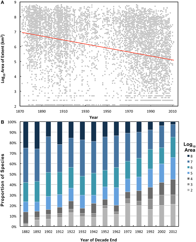
Figure 1. Geographic ranges (area of extent) of deep-sea species described each year. Only species with two or more records are shown. (A) Log-transformed range size for each species in the dataset (gray circles) with line of best fit (red line). (B) Proportion of species in each range-size category for each decade. Range size categories are indicated in the key.

TABLE 1

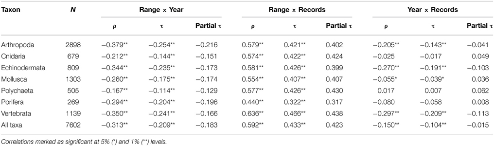
Table 1. Correlations (Spearman's ρ and Kendall's τ) and partial correlations (Partial τ) between range size, year described and number of records, for species of each taxon.

There was also a positive correlation (ρ = 0.59) between range size and number of records for species of all taxa (Table 1). This relationship was consistently stronger than that for range size and year described across all taxa (Table 1). Furthermore, when the number of records is controlled for by partial correlation analysis the correlation between range size and year of description is weakened, changing from τ = 0.21 to τ = 0.18 (Table 1). However, when taxa with fewer than six records are removed from the analysis (i.e., bottom 3 rows of Table 2), year of description becomes the strongest correlate of range size, greater than number of records.

TABLE 2

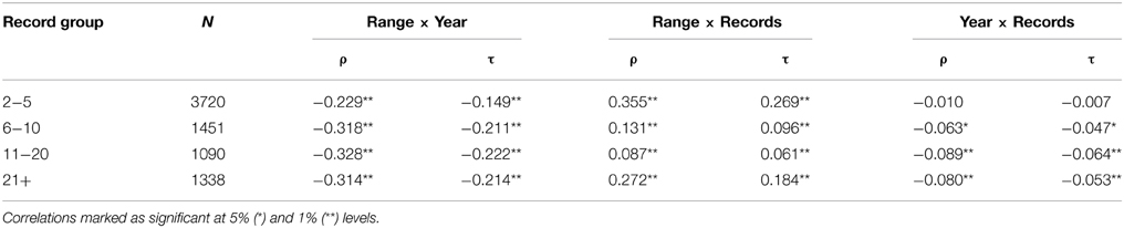
Table 2. Correlations (Spearman's ρ and Kendall's τ) between extent of occurrence, year described and number of records, for species grouped according to the number of records each has in the database.

There is a significant decline in average number of records per species described in each decade over the study period (Figure 2A; P < 0.001, J–T = –13.59). The correlation between the year described and the number of records was weak when all taxa are pooled, and not significant at the individual taxon level for the Cnidaria, Polychaeta, and Porifera (Table 1). Over the study period there is a decade on decade decrease in the proportion of species in the high records group, i.e., those with over 21 records (Figure 2B). There is a corresponding increase in the proportion of singleton species (those with only one record) in the first four decades after 1873 (R² = 0.91); however, the proportion of singletons remains relatively constant from 1912 onwards (R² = 0.05).

FIGURE 2

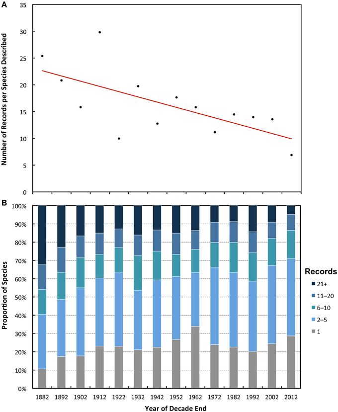
Figure 2. Decadal trends in the number of records in the database, including species with only one record. (A) Number of records in the database for species described in each decade, with line of best fit (red line). (B) Proportion of species categorized according to the number of records each species has. Record categories follow the key. Singletons are in gray.

There was no trend in the latitudinal distribution of species range midpoints over the study time period for species centered in the northern hemisphere, but for those in the southern hemisphere there was a small (range = 19°) decrease in latitude from the equator (Figure S1). Species with ranges spanning less than 20° of latitude were most abundant ~25° north and south of the equator (Figure 3).

FIGURE 3

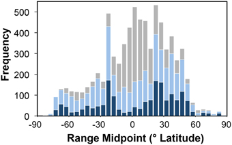
Figure 3. Latitudinal trends in species range sizes. Frequency of species latitudinal range midpoints occurring in each 5° latitudinal band. The number of small ranged species (latitudinal ranges < 20°) is shown as blue bars (light blue for species with < 6 records, dark blue for species with ≥6 records); gray bars show larger ranged species.

Discussion

Deep-sea species are generally thought to have broader distributional ranges than those of terrestrial and shallow-water species (McClain and Hardy, 2010), a view that is supported by the data presented here. Only 28% of species in the dataset have an EOO smaller than 10⁵ km², while a 39% have an EOO larger than 10⁷ km². Yet, we must question to what degree this preponderance of wide ranging species is actually generated by historical bias in species discovery. Species with narrow geographical ranges may be very difficult to sample in the deep sea, “leading to overestimation of the contribution of broadly distributed species to deep-sea biodiversity” (McClain and Hardy, 2010).

Our results are in general agreement with previous studies showing a negative correlation between species range size and the date of description (Gaston et al., 1995; Gibbons et al., 2005). However, the apparent conclusion that wide-ranging species are therefore more likely to be described first actually begs the question. The direction of causality between the variables cannot be assumed a priori and two scenarios could plausibly explain the correlation:

1. Wide-ranging species are described earlier because they tend to be encountered earlier,

or

2. Species that are described earlier simply accrue more records over time, giving them larger ranges.

The two mechanisms are not necessarily mutually exclusive, but understanding which has been most influential in shaping our current biodiversity records has implications for how we understand what is left to be discovered. Under scenario 1 it is expected that the average species range size will continue to decrease because species yet to be discovered have smaller ranges than those already discovered. In contrast, scenario 2 predicts that the observed decline in average range size is an artifact and given time records of species described in recent decades will accrue and the average range size will be elevated in line with those of previous decades.

The first causal relationship seems to be implicitly assumed in many previous studies, but Costello and Wilson (2011) argue that “the apparently narrower geographic and depth ranges for recently described species may be a consequence of when they were described rather than the reason for their later discovery.” This is a justifiable interjection and it may be especially true when EOO is used a definition of range size, as in this study. The relationship between range size and number of records is certainly the strongest in the overall correlation analysis (Table 1), although this is to be expected. The more records there are for a species the wider its geographic range, but is there a temporal component to this relationship?

If species range size was predominantly determined by the accumulation of records over time (scenario 2) it would be expected that there would be a strong negative correlation between the year of description and the number of records accumulated; the longer that a species has been known, the more likely it is to have been recorded. This does not seem to be the case, since the correlation between year described and number of records for individual species is the weakest of the three and is not even significant in several taxa (Table 1). Additionally, if accumulation of records was primarily driving the relationship there should be a steady decrease in the proportion of singleton species remaining in the older decades as they accumulate records over time, mirroring the trend for range size (gray bars in Figure 1B). However, the proportion of singletons has remained fairly static for the decades following 1912, indicating that there is a persistent proportion of rare species (Figure 2B).

There do not appear to be any latitudinal trends in the collection of new species over time, which might have biased the results (Figure S1). It has been hypothesized that species living at high latitudes will have wider geographic ranges because the greater seasonal changes in environment will mean that they are capable of exploiting a wider range of habitats. Previous attempts to detect this so-called “Rapoport's Rule” have tended to use the “Stevens method” or the “midpoint method” for plotting range size against latitude, but both are flawed and inherently biased toward producing opposite results (reviewed by Connolly, 2009). These problems largely come about because of geographical constraints on the placement of species range midpoints; the widest ranging species will necessarily have their midpoints nearer the equator. An alternative method is to identify the latitudes where small ranged species are most common, as presented in Figure 3. In contrast to the predictions of Rapoport's rule, the equatorial region has few narrow ranged species, while there are marked peaks at ~25° either side (both in absolute counts and as a proportion of species). Whether looking at species with only 2–5 records or >6 records the same trend holds (Figure 3), indicating that this is not just the result of poorly documented species.

Taken together, these results suggest that the primary reason for the decline in average species range size is that older species discovery has been biased toward species with large geographic ranges. The implication is that an increasing proportion of species that remain to be discovered will have smaller ranges and will therefore be more difficult to find. This difficulty may also be exasperated by their probable rarity. Previous studies have shown that wide ranging species also tend to be the most abundant (Glover et al., 2001, 2002), which might explain why there is an apparent effect of record accumulation over time (Figure 2A). If the wide ranging, more abundant species are discovered first then it is those species that will also be found more often because they are more abundant, not because they are old. Since relative abundance data are not available for each record in the database, it is difficult to explicitly evaluate this variable here. Even some rare species may be widely distributed in the deep-sea (Rex and Etter, 2010).

Another approach to estimating the effect of the historical bias in species discovery is to compare the species range size frequency distribution (RSFD) observed here with a theoretical null distribution. The two null distributions most commonly suggested are the log-normal and more recently the logit-normal distribution (Gaston, 1998; Williamson and Gaston, 1999, 2005). The RSFDs of deep-sea species in our dataset are strongly right skewed (Figure 4A), even when species with less than 6 records are removed (Figure 4B). Neither log nor logit-transformations of the data are able to normalize theses distributions, resulting in a left skew (Figures 4C–F). This departure from normality has previously been interpreted as a lack of wide- or narrow-ranged species relative to expectation (Gaston et al., 2005). There is a some excursion from normality in the smaller range size classes resulting from undersampled species (compare distributions when species with < 6 records are excluded in Figures 4D,F). However, the bulk of the departure is in the largest range size classes, which seems to bear out the conclusion above; namely that wide-ranged are overrepresented in our current catalog of diversity.

FIGURE 4

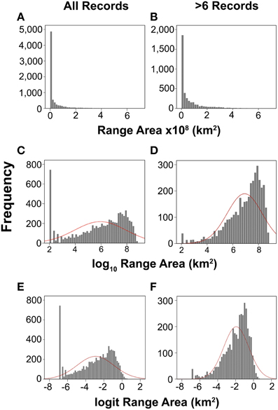
Figure 4. Range size frequency diagrams for all species (A,C,E) and only species with 6 or more records (B,D,F). Dashed red lines show normal distribution with parameters derived from the data.

The traditional view that deep-sea taxa tend to have wider ranges than those in shallow habitats is used to support lower estimates of global marine species richness (e.g., Costello et al., 2012). The inference is that total deep-sea species richness is less than that of shallow habitats because its species are more widely distributed. Rex and Etter (2010) come to a similar conclusion after reviewing relevant studies. Since shallow water species richness is relatively well-known, then it is possible to constrain the contribution of deep-sea species to global species richness. This type of comparative reasoning relies on correctly gauging macroecological relationships, but the question of whether total deep-sea species richness is greater or less than that of shallow waters has not been rigorously tested (McClain and Schlacher, 2015). In reviewing available data, Gray (2002) concluded that species density is similar in coastal and deep sediments at large scales, with deep-sea being more species rich at local scales. If the proportion of narrow-ranged species is underestimated (as suggested here), then conservative estimates of species richness should be revised upwards (e.g., Poore and Bruce, 2012).

Any analysis of the range-size distribution of deep-sea taxa is complicated by the problem of cryptic species, i.e., morphologically identical species that are genetically distinct. Initial studies have found an unexpectedly high degree of cryptic species in the deep sea. For example polychaete and nematode morphotypes show geographic distributions of 1000–3000 km in the abyssal Pacific, but genetic analysis suggests that there is little gene flow across these vast ranges (Smith et al., 2008). Cryptic species are so common among the deep-sea peracarid crustaceans (one of the most speciose deep-sea taxa) that a recent analysis found few (if any) truly wide-ranging species in this taxon (Brandt et al., 2012). The preponderance of cryptic species suggests that we are currently overestimating the proportion of wide-ranging deep-sea species and underestimating the total species richness of the deep sea. Furthermore, many of the extremely wide-ranged species described from earlier decades (Figure 1B) may in fact be cryprtic species complexes, inflating the change in mean species range size over the study period (Figure 1A).

Conclusions

There has been a historical bias in the documentation of deep-sea biodiversity toward apparently wide-ranging species. Our current records seem to represent the “low-hanging fruit” in terms of species discovery in the deep sea and the bulk of undiscovered species are likely to have relatively narrow geographical distributions. This is not surprising; deep-sea biology is a fairly young discipline. Only a decade ago a typical survey of the abyssal plains and basins (54% of Earth's surface) would typically find that 90% of the infaunal species collected were new to science (Ebbe et al., 2010). This staggering figure has changed little for groups like nematodes, isopods, and copepods (Seifried, 2004; Ebbe et al., 2010), some of the most abundant components of deep-sea benthic diversity. Such high rates of discovery suggest that current catalogs are far from complete and therefore estimates of total species richness are necessarily uncertain (Bebber et al., 2007).

While the dataset used here only crudely approximates actual species ranges in the form of possible EOO, it is the best available on such a global scale. It should therefore be viewed as a baseline against which we can further test hypotheses in deep-sea biogeography. The construction of a specific deep-sea species database is currently underway (Glover et al., 2015) and will greatly help with tackling the question of deep-sea species richness. Ultimately, high-quality taxon-specific geographic data will be required to elucidate fine scale patterns of species range sizes (e.g., Brandt et al., 2012). Until such data become available we caution against over-confidence in our current catalogs of deep-sea biodiversity. Far from being a “known unknown,” we argue (with McClain and Schlacher, 2015) that total deep-sea species richness cannot be currently estimated with confidence.

Conflict of Interest Statement

The authors declare that the research was conducted in the absence of any commercial or financial relationships that could be construed as a potential conflict of interest.

Acknowledgments

The impetus and for this paper came from a conversation on Twitter between NDH and Tom Webb (University of Sheffield). Mike Flavell (OBIS Data Manager) and Wim Decock (WoRMS data management team) provided assistance in accessing data. The authors are greatly indebted to the numerous contributors and curators of these databases. We are grateful to both reviewers, whose thoughtful comments improved the clarity of the manuscript. NDH was supported by a postdoctoral fellowship from the Plymouth University Marine Institute.

Supplementary Material

The Supplementary Material for this article can be found online at: https://www.frontiersin.org/article/10.3389/fmars.2015.00061

Figure S1. Species latitudinal range midpoints plotted against year described, for the northern and southern hemispheres. Red lines show line of best fit for data in each hemisphere.

References

Allsopp, P. G. (2003). Probability of describing an Australian scarab beetle: influence of body size and distribution. J. Biogeogr. 24, 717–724. doi: 10.1046/j.1365-2699.1997.00154.x

CrossRef Full Text | Google Scholar

Appeltans, W., Ahyong, S. T., Anderson, G., Angel, M. V., Artois, T., Bailly, N., et al. (2012). The magnitude of global marine species diversity. Curr. Biol. 22, 2189–2202. doi: 10.1016/j.cub.2012.09.036

PubMed Abstract | CrossRef Full Text | Google Scholar

Bebber, D. P., Marriott, F. H. C., Gaston, K. J., Harris, S. A., and Scotland, R. W. (2007). Predicting unknown species numbers using discovery curves. Proc. Biol. Sci. 274, 1651–1658. doi: 10.1126/science.149.3686.880

PubMed Abstract | CrossRef Full Text | Google Scholar

Brandt, A., Błażewicz-Paszkowycz, M., Bamber, R., Mühlenhardt-Siegel, U., Malyutina, M., Kaiser, S., et al. (2012). Are there widespread peracarid species in the deep sea (Crustacea: Malacostraca)? Pol. Polar Res. 33, 139–162. doi: 10.2478/v10183-012-0012-5

CrossRef Full Text | Google Scholar

Carney, R. S. (2005). Zonation of deep biota on continental margins. Oceanog. Mar. Biol. 43, 211–278. doi: 10.1201/9781420037449.ch6

PubMed Abstract | CrossRef Full Text | Google Scholar

Collen, B., Purvis, A., and Gittleman, J. L. (2004). Biological correlates of description date in carnivores and primates. Glob. Ecol. Biogeog. 13, 459–467. doi: 10.1111/j.1466-822X.2004.00121.x

CrossRef Full Text | Google Scholar

Connolly, S. R. (2009). “Macroecological theory and the analysis of species richness gradients,” in Marine Macroecology, eds J. D. Witman and K. Roy (London: University of Chicago Press), 279–309.

Google Scholar

Costello, M. J., May, R. M., and Stork, N. E. (2013a). Can we name earth's species before they go extinct? Science 339, 413–416. doi: 10.1126/science.1230318

PubMed Abstract | CrossRef Full Text | Google Scholar

Costello, M. J., May, R. M., and Stork, N. E. (2013b). Response to comments on “can we name earth's species before they go extinct?” Science 341, 237. doi: 10.1126/science.1237381

PubMed Abstract | CrossRef Full Text | Google Scholar

Costello, M. J., Wilson, S., and Houlding, B. (2012). Predicting total global species richness using rates of species description and estimates of taxonomic effort. Syst. Biol. 61, 871–883. doi: 10.1093/sysbio/syr080

PubMed Abstract | CrossRef Full Text | Google Scholar

Costello, M. J., and Wilson, S. P. (2011). Predicting the number of known and unknown species in European seas using rates of description. Glob. Ecol. Biogeog. 20, 319–330. doi: 10.1111/j.1466-8238.2010.00603.x

CrossRef Full Text | Google Scholar

Ebbe, B., Billett, D. S. M., Brandt, A., Glover, A. G., Keller, S., Malyutina, M., et al. (2010). “Diversity of abyssal marine life,” in Life in the World's Oceans, ed A. McIntyre (Chichester, UK: Wiley-Blackwell), 139–160.

Google Scholar

Gage, J., and Tyler, P. A. (1992). Deep-Sea Biology. Cambridge, UK: Cambridge University Press.

Google Scholar

Gaston, K. J. (1998). Species-range size distributions: products of speciation, extinction and transformation. Philos. Trans. R. Soc. Lond. B Biol. Sci. 353, 219–230. doi: 10.1098/rstb.1998.0204

CrossRef Full Text | Google Scholar

Gaston, K. J., Blackburn, T. M., and Loder, N. (1995). Which species are described first? the case of North American butterflies. Biodivers. Conserv. 4, 119–127. doi: 10.1007/BF00137780

CrossRef Full Text | Google Scholar

Gaston, K. J., Davies, R. G., Gascoigne, C. E., and Williamson, M. (2005). The structure of global species-range size distributions: raptors & owls. Glob. Ecol. Biogeog. 14, 67–76. doi: 10.1111/j.1466-822X.2004.00123.x

CrossRef Full Text | Google Scholar

Gaston, K. J., and Fuller, R. A. (2009). The sizes of species' geographic ranges. J. Appl. Ecol. 46, 1–9. doi: 10.1111/j.1365-2664.2008.01596.x

CrossRef Full Text | Google Scholar

Gibbons, M. J., Richardson, A. J. V., Angel, M., Buecher, E., Esnal, G., Boettger-Schnack, R., et al. (2005). What determines the likelihood of species discovery in marine holozooplankton: is size, range or depth important? Oikos 109, 567–576. doi: 10.1111/j.0030-1299.2005.13754.x

CrossRef Full Text | Google Scholar

Glover, A. G., Higgs, N. D., and Horton, T. (2015). World Register of Deep-sea Species. Available online at: http://www.marinespecies.org/deepsea

Glover, A. G., Paterson, G., Bett, B. J., Gage, J. D., Sibuet, M., Sheader, M., et al. (2001). Patterns in polychaete abundance and diversity from the Madeira Abyssal Plain, northeast Atlantic. Deep Sea Res. Part I Oceanogr. Res. Pap. 48, 217–236. doi: 10.1016/S0967-0637(00)00053-4

CrossRef Full Text | Google Scholar

Glover, A. G., Smith, C. R., Paterson, G., Wilson, G., Hawkins, L., and Sheader, M. (2002). Polychaete species diversity in the central Pacific abyss: local and regional patterns, and relationships with productivity. Mar. Ecol. Prog. Ser. 240, 157–170. doi: 10.3354/meps240157

CrossRef Full Text | Google Scholar

Grassle, J. F., and Maciolek, N. J. (1992). Deep-sea species richness: regional and local diversity estimates from quantitative bottom samples. Am. Nat. 139, 313–341. doi: 10.1086/285329

CrossRef Full Text | Google Scholar

Gray, J. S. (1994). Is deep-sea species diversity really so high: species diversity of the Norwegian continental shelf. Mar. Ecol. Prog. Ser. 112, 205–209. doi: 10.3354/meps112205

CrossRef Full Text

Gray, J. S. (2002). Species richness of marine soft sediments. Mar. Ecol. Prog. Ser. 244, 285–297. doi: 10.3354/meps244285

CrossRef Full Text | Google Scholar

Hessler, R. R., and Sanders, H. L. (1967). Faunal diversity in the deep sea. Deep Sea Res. Oceanogr. Abstr. 14, 65–78. doi: 10.1016/0011-7471(67)90029-0

CrossRef Full Text | Google Scholar

Jonckheere, A. R. (1954). A distribution-free k-sample test against ordered alternatives. Biometrika 41, 133–145. doi: 10.1093/biomet/41.1-2.133

CrossRef Full Text | Google Scholar

Lambshead, P. J. D., and Boucher, G. (2003). Marine nematode deep−sea biodiversity–hyperdiverse or hype? J. Biogeogr. 30, 475–485. doi: 10.1046/j.1365-2699.2003.00843.x

CrossRef Full Text | Google Scholar

Legendre, P., and Legendre, L. (1998). Numerical Ecology. New York, NY: Elsevier.

Google Scholar

May, R. (1992). Bottoms up for the oceans. Nature 357, 278–279. doi: 10.1038/357278a0

CrossRef Full Text | Google Scholar

McClain, C. R., and Hardy, S. M. (2010). The dynamics of biogeographic ranges in the deep sea. Proc. R. Soc. B 277, 3533–3546. doi: 10.1098/rspb.2010.1057

PubMed Abstract | CrossRef Full Text | Google Scholar

McClain, C. R., and Schlacher, T. A. (2015). On some hypotheses of diversity of animal life at great depths on the sea floor. Mar. Ecol. doi: 10.1111/maec.12288. [Epub ahead of print].

CrossRef Full Text | Google Scholar

Mora, C., Rollo, A., and Tittensor, D. P. (2013). Comment on “Can we name Earth's species before they go extinct?.” Science 341, 237. doi: 10.1126/science.1237254

PubMed Abstract | CrossRef Full Text | Google Scholar

Mora, C., Tittensor, D. P., Adl, S., Simpson, A. G. B., and Worm, B. (2011). How many species are there on Earth and in the ocean? PLoS Biol. 9:e1001127. doi: 10.1371/journal.pbio.1001127

PubMed Abstract | CrossRef Full Text | Google Scholar

OBIS. (2015). Intergovernmental Oceanographic Commission of UNESCO. Available online at: http://www.iobis.org

Pimm, S. L., Jenkins, C. N., Abell, R., Brooks, T. M., Gittleman, J. L., Joppa, L. N., et al. (2014). The biodiversity of species and their rates of extinction, distribution, and protection. Science 344:1246752. doi: 10.1126/science.1246752

PubMed Abstract | CrossRef Full Text | Google Scholar

Poore, G. C. B., and Bruce, N. L. (2012). Global diversity of marine isopods (except asellota and crustacean symbionts). PloS One 7:e43529. doi: 10.1371/journal.pone.0043529

PubMed Abstract | CrossRef Full Text | Google Scholar

Poore, G. C. B., and Wilson, G. D. F. (1993). Marine species richness. Nature 361, 597–598. doi: 10.1038/361597a0

CrossRef Full Text | Google Scholar

Rex, M. A., and Etter, R. J. (2010). Deep-sea Biodiversity. Cambridge, MA: Harvard University Press.

Google Scholar

Sars, G. O. (1873). On Some Remarkable Forms of Animal Life from the Great Deeps Off the Norwegian Coast. Christiania: Brøgger & Christie.

Google Scholar

Seifried, S. (2004). The importance of a phylogenetic system for the study of deep-sea harpacticoid diversity. Zool. Stud. 43, 435–445.

Google Scholar

Smith, C. R., Paterson, G., Lambshead, P. J. D., Glover, A. G., Rogers, A. D., Gooday, A. J., et al. (2008). Biodiversity, Species Ranges, and Gene Flow in the Abyssal Pacific Nodule Province. International Seabed Authority Technical Study, No. 3. Jamaica.

Stork, N. E., Grimbacher, P. S., Storey, R., Oberprieler, R. G., Reid, C., and Adam Slipinski, S. A. (2008). What determines whether a species of insect is described? Evidence from a study of tropical forest beetles. Insect Conserv. Divers. 1, 114–119. doi: 10.1111/j.1752-4598.2008.00016.x

CrossRef Full Text | Google Scholar

Watling, L., Guinotte, J., Clark, M. R., and Smith, C. R. (2012). A proposed biogeography of the deep ocean floor. Prog. Oceanogr. 111, 99–112. doi: 10.1016/j.pocean.2012.11.003

CrossRef Full Text | Google Scholar

Webb, T. J., Berghe, E. V., and O'Dor, R. (2010). Biodiversity's big wet secret: the global distribution of marine biological records reveals chronic under-exploration of the deep pelagic ocean. PLoS ONE 5:e10223. doi: 10.1371/journal.pone.0010223

PubMed Abstract | CrossRef Full Text | Google Scholar

Williamson, M., and Gaston, K. J. (1999). A simple transformation for sets of range sizes. Ecography 22, 674–680. doi: 10.1111/j.1600-0587.1999.tb00516.x

CrossRef Full Text | Google Scholar

Williamson, M., and Gaston, K. J. (2005). The lognormal distribution is not an appropriate null hypothesis for the species-abundance distribution. J. Anim. Ecol. 74, 409–422. doi: 10.1111/j.1365-2656.2005.00936.x

CrossRef Full Text | Google Scholar

WoRMS Editorial Board (2015). World Register of Marine Species. Available online at: http://www.marinespecies.org (Accessed September 19, 2014).

Zapata, F. A., and Robertson, D. R. (2007). How many species of shore fishes are there in the Tropical Eastern Pacific? J. Biogeogr. 34, 38–51. doi: 10.1111/j.1365-2699.2006.01586.x

CrossRef Full Text | Google Scholar