Optical Signatures of Dissolved Organic Matter Transformation in the Global Ocean

Introduction

Dissolved organic matter (DOM) represents one of the largest pools of carbon in the global biosphere (Hansell, 2013; Hansell and Carlson, 2015). It is well understood that DOM in the ocean gradually remineralizes over time, but it is unclear what governs the rates of remineralization, particularly in the deep ocean (Arístegui et al., 2002; Carlson and Hansell, 2015). The structural transformations that occur during remineralization are not well understood, however the characterization of the composition of organic matter with an eye toward determining how to detect and quantify the more labile and refractory components of DOM is critical for understanding the physico-chemical properties and residence time of the DOM pool. Optical properties of DOM, including UV-visible absorption spectra and fluorescence spectra, provide one means of characterizing the composition of DOM without subjecting the samples to concentration processes that can be selective (Green et al., 2014).

Our previous work has quantified the distribution of chromophoric DOM (CDOM) in the global ocean using UV-Visible absorption spectroscopy (Nelson and Siegel, 2013). We have postulated new production of CDOM in the surface (Nelson et al., 1998) and deep ocean (Nelson et al., 2010). Diagenesis-related changes in absorption properties of CDOM have also been documented (Nelson et al., 2007), and the relationship between CDOM and DOC in the global ocean suggests that CDOM absorption in the deep ocean represents a refractory component of the DOM (Nelson et al., 2010). In the present study, the optical properties of DOM are characterized in order to further our understanding of the different sub-pools of DOM and how they are transformed by remineralization or photodegradation (Jaffe et al., 2008; Carlson and Hansell, 2015). The present analysis is focused on distributions and processes in the open ocean, away from the input of terrestrial material on the annual scale, as this represents the majority of the global surface and deep ocean.

Distribution of CDOM (as quantified as the UV absorption coefficient of filtered seawater in the solar waveband) is characterized by surface minima, particularly in the stratified subtropics, due to solar bleaching (Nelson et al., 1998, 2010; Swan et al., 2012). At the base of the mixed layer in situ production can overcome bleaching, resulting in a local maximum in the CDOM profile (Nelson et al., 1998, 2010). Below the euphotic zone there can be a local minimum in the intermediate or subtropical mode waters followed by an increase in the CDOM absorption coefficient in the main thermocline (Nelson et al., 2007, 2010). Local surface maxima can occur in regions of high primary productivity (Nelson et al., 2007). Regional differences in the surface distribution of CDOM reflect upwelling zones, major river inputs, and much greater CDOM absorption coefficients in the mid to high latitudes in the northern hemisphere (Siegel et al., 2002). In the main thermocline and below, CDOM is strongly correlated with apparent oxygen utilization (AOU), except in the Atlantic, where CDOM abundance varies little over the range of AOU present, and CDOM is much more abundant at low AOU than in the Pacific or Indian Ocean basins (Nelson and Siegel, 2013). The pattern in the Atlantic is linked to more rapid overturning circulation and input of preformed CDOM via the Arctic (Nelson et al., 2010; Jørgensen et al., 2011).

CDOM in the ocean changes its optical properties over time. Previous work has observed increases in DOC-specific absorption coefficient and the exponential slope parameter in “older” water masses, as assessed by CFC-12 ventilation age (Nelson et al., 2007) and AOU (Nelson et al., 2010). The distribution patterns of CDOM light absorption reflect balances between the production of CDOM and its degradation by solar bleaching, modulated by overturning circulation and the presence of preformed CDOM (Nelson et al., 2010; Nelson and Siegel, 2013). This interpretation implies that there are two autochthonous sources of CDOM, one located in the surface productive layer (Nelson et al., 2004), and one located primarily in the main thermocline (Nelson et al., 2010). The CDOM produced by these two local sources may have significantly different composition, which is not readily revealed by absorption properties alone. Studies of “new” CDOM production in the laboratory have identified DOM with discrete peaks in UV absorbance (Steinberg et al., 2004) that do not resemble the canonical CDOM absorption spectra that resemble terrestrial humic material absorption spectra (Del Vecchio and Blough, 2004), suggesting the existence of processes that “humify” freshly produced DOM. Microbial cultures have been found to produce labile UV absorbing or fluorescing CDOM (Rochelle-Newall and Fisher, 2002; Nelson et al., 2004; Nieto-Cid et al., 2006), and long-lived, visible fluorescing material (Jørgensen et al., 2014), further suggesting a microbial link to transformation of DOM in situ.

In the present study, we are taking a multiparameter approach toward optical characterization by using absorption and fluorescence properties to examine patterns of variability related to transformations of organic matter in the open ocean. Fluorescence of CDOM has also been used to assess the distribution of chromophoric compounds in the ocean (Chen and Bada, 1992; Determann et al., 1996; Yamashita and Tanoue, 2009; Andrew et al., 2013). While fluorescent substances are a subset of the chromophores in DOM (Stedmon and Nelson, 2015), fluorescence spectroscopy, in particular excitation-emission matrix spectroscopy (EEM; Coble, 2007) can be used to characterize aspects of the chemical composition of CDOM over and above the light absorption spectra.

Fluorescence analysis identifies essentially two major categories of dissolved organic material in the ocean: materials that have fluorescence emission maxima in the UVA that are similar to aromatic amino acids (T, N, and B regions, Table 1, Yamashita and Tanoue, 2003), and humic-like materials that have fluorescent emission maxima in the visible (A, C, and M regions, (Table 1, Stedmon and Nelson, 2015). According to this paradigm, depth distribution of fluorescence parameters reflects freshly produced material near the surface, and humic material at depth that represents aged terrestrial or marine-origin material (Jørgensen et al., 2011; Catalá et al., 2015). Experimental results have highlighted the UV absorption characteristics of freshly produced CDOM of microbial or other heterotroph origin as well (e.g., Steinberg et al., 2004; Suksomjit et al., 2009). Strong links between UV absorption or fluorescence properties, and remineralization-related variables such as AOU suggest a link between microbial degradation of DOM in the thermocline and deep ocean, and production of chromophoric DOM (Murphy et al., 2008; Yamashita and Tanoue, 2008; Nelson et al., 2010; Jørgensen et al., 2011; Catalá et al., 2015; Lonborg et al., 2015).

TABLE 1

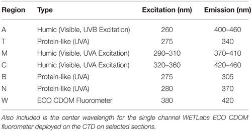
Table 1. Central locations for the canonical fluorescence regions modified from Coble (2007) by Stedmon and Nelson (2015).

In the present study we build upon previous work on CDOM absorption properties in the open ocean along the Repeat Hydrography sections (Nelson et al., 2007, 2010; Swan et al., 2009) by adding fluorescence characterization to the parameters measured, using approaches analogous to those used by Jørgensen et al. (2011) and Catalá et al. (2015). Fluorescence EEM spectroscopy provides another dimension to CDOM analysis by identifying one or more fluorophores that may absorb light in a single waveband. In particular we are attempting to identify the nature and location in the water column of processes that produce long-lived chromophores in the ocean. Our sampling area excludes the continental shelves and areas directly influenced by terrestrial input, which we believe gives us the best chance at identifying autochthonous processes.

Methods and Materials

Hydrographic Data and Sampling

We collected samples on six sections of the U.S. CO₂/CLIVAR Repeat Hydrography Project (Feely et al., 2005) between 2008 and 2013, spanning the Indian, Pacific, Southern and Atlantic Oceans (Figure 1). Our typical sampling frequency for CDOM was once daily (ca. 1° of latitude on meridional sections), with samples collected throughout the whole water column (Nelson et al., 2010). The hydrographic parameters sampled by other researchers included CTD temperature, salinity, dissolved oxygen, primary nutrients (NO₃, PO₄, and SiO₄), inorganic carbon concentrations (nominally pCO₂ and DIC), CFC species (CFC-11, CFC-12, and CFC-13), and dissolved organic carbon (DOC) concentrations (Feely et al., 2004). WOCE standard protocols were used for all hydrographic measurements. Details of the measurement protocols, cruise narratives and data sets are available at the Repeat Hydrography Program website (http://cchdo.ucsd.edu/). Computations of neutral density and AOU were performed using Ocean Data View (Schlitzer, 2008).

FIGURE 1

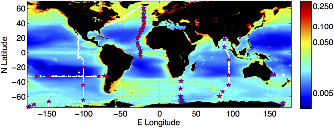
Figure 1. Distribution of the climatology of surface water colored dissolved and detrital material (CDM) from ocean color observation, and locations of the field observations used in the present study. CDM is quantified as the sum of the absorption coefficient (m⁻¹) of CDOM and the absorption coefficient of non-phytoplankton (detrital) particles (m⁻¹) at 443 nm. The surface CDM field was derived from the SeaWiFS mission mean of the Garver-Siegel-Maritorena algorithm CDM product (Maritorena et al., 2002; Siegel et al., 2002). Field observations were collected on meridional transects A16N (Iceland to Brazil, 2013), P18 (Baja California to the ice edge, 2007/2008), I8S/I9N (Southern and Indian Oceans near 90°E, Feb–Apr 2007, I6 (Cape Town to the ice edge, 2009), and zonal transects S4P (Ross Sea to Bellingshausen Sea, 2011), and P6 (Brisbane—Valparaiso, 2009/2010). White dots indicate all locations at which hydrographic data were collected; red stars indicate locations at which EEMs were measured from water samples.

Sample Preparation and Storage

Water samples were prepared for spectrophotometric analysis according to established methods (Nelson et al., 1998, 2004). Samples were drawn from Niskin bottles into acid-washed and ultrapure water-rinsed amber glass vials with Teflon liner caps. The samples were then filtered using 0.2 μm Nuclepore polycarbonate membrane filters that had been rinsed with ultrapure water to remove any possible absorbing contaminants. Samples for EEM analysis were shipped on ice to UCSB and kept sealed, refrigerated at 4°C, and in the dark until processing (Nelson et al., 2007). Time until processing ranged from several months to 2 years. Stability of CDOM samples has been assessed by long term storage (results for absorption properties reported in Swan et al., 2009). Some samples proved to have contamination issues related to storage and were discarded (see below).

CDOM Absorption Spectroscopy

CDOM absorption was quantified as the absorption coefficient at 325 nm of the dissolved materials as determined using a WPI UltraPath liquid waveguide spectrophotometer (Miller et al., 2002) following previously developed methods (Nelson et al., 2007; Swan et al., 2009). Absorption spectra of the filtered seawater samples equilibrated to room temperature were recorded against MilliQ water (Millipore) in the 1.984 m liquid waveguide spectrophotometer. Absorption spectra were corrected for refractive index differences between samples and ultrapure water using an empirical method based on salinity (Nelson et al., 2007). The absorption coefficient at 325 nm (calculated as absorbance divided by path length, multiplied by 2.303 to convert to natural log units) operationally represents CDOM abundance. Duplicate samples collected from the same Niskin on the I8S/I9N sections showed root mean square differences of <4% at 325 nm.

CDOM absorption spectra typically exhibit logarithmic-scale decline with wavelength (Figures 2B,D,F). Spectral slope parameter (S_snlf, units of nm⁻¹), the parameter of an exponential equation that best fits the CDOM spectrum over a discrete wavelength interval, was computed for each spectrum over two wavelength ranges in the ultraviolet (Helms et al., 2008) using a least-squares non-linear curve fit method (Stedmon and Markager, 2001).

FIGURE 2

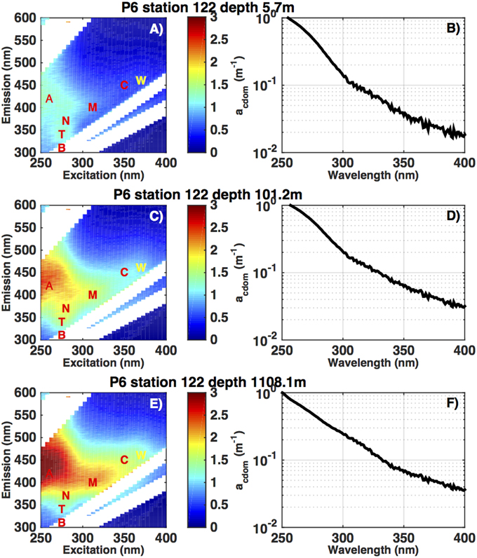
Figure 2. Excitation-Emission Matrix (EEM) fluorescence spectra (ppb QSE) and absorption spectra (m⁻¹) from a depth profile in the subtropical South Pacific (32S, 149W), on the CLIVAR P6 section in December 2009. The letters in panels (A,C,E) refer to the excitation-emission coordinates of defined fluorescence regions. A, M, and C are defined by their position as humic-like fluorescence and T and B are amino acid-like fluorescence signatures (Coble 1996). The CTD ECO fluorometer measures fluorescence in a small defined band, near the C region, indicated by the W. The colorbar refers to increasing fluorescence (ppb QSE) from blue to red. Panels (B,D,F) show the corresponding CDOM absorbance spectra at 325 nm, from 250 to 400 nm.

Fluorescence Spectral Analysis

On selected samples (profile locations shown as stars in Figure 1) we performed EEM fluorescence analysis (Coble, 1996; Nelson and Coble, 2010). This measurement is a compilation of fluorescence emission spectra run sequentially with a range of excitation wavelengths, resulting in a two dimensional dataset for each sample (Figures 2A,C,E).

Filtered seawater samples for EEM analysis were allowed to equilibrate to room temperature and subsequently analyzed in a Horiba Jobin-Yvon Fluoromax-4 fluorescence spectrophotometer in 1 cm quartz cells. Excitation and emission slit widths were set to 5 nm. Emission scans were recorded in ratio mode (fluorescence/reference intensity) from 300 to 600 nm, every 2 nm, with sequential excitation every 5 nm between 250 and 400 nm. Analysis of a single sample takes approximately 22 min. Before and after-measurements (not shown) indicated the samples warmed up less than 0.1°C during analysis, so no further temperature control was attempted. Ultrapure water blanks were run each session and were subtracted from the sample EEMs during data processing. The EEMs were corrected for detector response (both emission and reference detectors) using spectral correction factors provided by the manufacturer.

Each EEM was normalized to the equivalent fluorescence of a known concentration of quinine sulfate dissolved in sulfuric acid. Before each batch of EEM samples were run each day, the fluorescence emission spectrum (300–500 nm, excitation 348 nm) of a ~4–5 ppb quinine sulfate standard solution was measured. Subsequent EEM samples were normalized to the quinine sulfate fluorescence at the quinine sulfate excitation/emission maximum (348/450 nm) and the concentration of the standard, resulting in an EEM with units of ppb quinine sulfate equivalent (ppb QSE) that can be compared to other measurements.

In Figures 2A,C,E we provide an example of fluorescence EEMs from one profile in the subtropical South Pacific (32S, 149W). Highlighted on this graph in red letters are the nominal positions of the fluorescence regions typically highlighted in discussions of EEM data (cf. Coble, 1996). Regions A and C are thought to be most closely related to terrestrial humic materials, region M is thought to represent a combination of terrestrial and marine humic material (Murphy et al., 2008), and the T and B regions are clearly attributable to the fluorescence of aromatic amino acids (Yamashita and Tanoue, 2003; Jørgensen et al., 2011). The white areas on the EEM plots are areas where the fluorescence of the sample is overwhelmed by Raman or Rayleigh scattering (Zepp et al., 2004). With the instrument and bandwidth settings used in the present study we could not resolve the B region due to Raman scattering, so we do not treat this area separately. We found the T and N regions highly correlated so we only present results from the T region in comparison plots. Figure 2 clearly shows the decline in fluorescence intensity from the deep ocean to the surface that is typical of subtropical CDOM fluorescence or absorption profiles (Nelson et al., 2010), and the relative importance of the T region can be seen to be higher at 100 m and near the surface than at depth.

We analyzed a total of 730 samples using EEM spectroscopy, representing 69 discrete stations, on the six CLIVAR cruises occupied as part of this study. EEM spectra were subjected to additional quality control mainly involving inspecting the collected data for artifacts that usually resulted from bubbles on the cuvette windows. Other samples exhibited fluorescence in the T-B region (Figure 2) that exceeded reasonable values based on other samples in the profile. These samples were judged to be contaminated and were discarded. Samples failing these tests were excluded from EOF analysis (see below) and from fluorescent region intensity analysis if the part of the EEM affected by bubbles was in the region. This resulted in a data set of over 500 samples for each comparison (see Results).

WETLabs CDOM Fluorometer

On the I8S/I9N, P6, and A16N sections we deployed a WETLabs ECO CDOM fluorometer (6000 m rated) on the main CTD rosette. This instrument is a single channel fluorometer with excitation at 380 ± 10 nm and emission detection at 420 ± 20 nm, closest to the C region of the EEM (Table 1). Data were recorded in volts. Sensitivity of the instrument varied with gain settings and calibration drift. To facilitate comparison with the EEM data, we devised a linear transfer function for each cruise (over which gain and calibration were assumed to be constant) to transfer the quinine-sulfate scaled EEM data (ppb QSE) from the W region (Figure 2) to the ECO fluorometer data. The fluorescence of EEM samples averaged over the excitation/emission region of the ECO fluorometer were regressed against the fluorometer voltage at the depth of the sample, averaged over 2 m depth. The resulting slope average was applied to the fluorometer data on a cruise-by-cruise basis to result in calibrated (ppb QSE) fluorescence data that can be compared between cruises and with EEM data. For the purpose of discussion, these single channel data will be referred to as “F_cdom.”

Analysis of EEM Data by Empirical Orthogonal Functions

We used the technique of empirical orthogonal function (EOF) analysis (e.g., Preisendorfer and Mobley, 1988) to examine the variability of fluorescence EEM data. EOF analysis is a purely empirical process that decomposes the variance of a dataset into a discrete number of constant eigenvectors (basis functions or “modes”) that have the same dimensions as a single example of the data, and variable expansion coefficients or “amplitudes” which are one-dimensional. An individual data “point” (i.e., an EEM) can be reconstructed as the sum of the products of the modes, their corresponding amplitudes, and an eigenvalue for each mode that represents the total variance in the data set accounted for by the mode. The fractional contribution to the total variance of the dataset represented by each mode can be computed, and is generally used to discriminate between significant and insignificant modes of variability. We implemented the EOF analysis in Matlab by reshaping the three-dimensional matrix of multiple EEMs to a two dimensional field, and computing the largest eigenvalues and eigenvectors of the covariance matrix using the built-in Matlab function eigs(). Contribution of each eigenvector to the total variance was calculated as the eigenvalues divided by the sum of the eigenvalues. In the present study we only consider modes of variability that account for more than 1% of the total variance of the dataset, which corresponded to the first three eigenvectors computed.

Results

Distribution of CDOM and Fluorescence Properties

The samples collected for this study came from a latitude range spanning 60N–60S (Figure 1), and depth ranges from the surface to over 5000 m at the ocean floor. We here present data from all of the major ocean basins away from the continental shelves excepting the North Pacific and the Arctic Oceans. Despite the range of locations and ecosystems sampled there were some factors common to most profiles that are highlighted first.

An example of CDOM and F_cdom profiles is given in Figure 3. This profile is from the same station from which the Figure 2 example EEMs and absorption spectra were taken. In this picture, discrete bottle sample CDOM absorption at 325 nm (black dots) are compared to the vertical profile of temperature (red line) and F_cdom (blue line). In the main thermocline (~500–1500 m at this station) and below, visible light fluorescence measured by the CDOM fluorometer (F_cdom) is well correlated with CDOM UV absorption a_g(325 nm). Between 500 and 250 m F_cdom remains roughly constant, then decreases monotonically toward the surface. The CDOM UV absorption profile instead shows two maxima in the depth range between 500 m and the surface: a broad shallow maximum centered near 350 m and a sharper maximum near 75 m. The surface mixed layer has the lowest CDOM absorption and fluorescence due to solar bleaching.

FIGURE 3

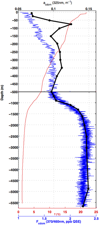
Figure 3. Profiles of temperature (°C, red line), CDOM absorption coefficient at 325 nm (black dots), and F_cdom from the ECO fluorometer (ppb QSE, blue line) from a depth profile in the subtropical South Pacific (32S, 149W), on the CLIVAR P6 section in December 2009. Note the scale change at 500 m.

This pattern with a local subsurface CDOM maximum that does not correlate with F_cdom present was common to most open ocean areas covered in this study. Figure 4 shows a scatter plot of F_cdom vs. a_g(325 nm) from samples collected on the I8S/I9N section in the Indian Ocean, covering the ice edge to the Bay of Bengal (Figure 1). Color codes show the depth range of the samples. Samples collected in and below the main thermocline (blue dots) exhibit a strong linear relationship between F_cdom and a_g(325 nm) (R² = 0.86), but this pattern breaks down shallower in the water column with a very weak relationship in the top 200 m where the a_g(325 nm) profile has the subsurface maximum peak highlighted in Figure 3. Similar scatter plots for other ocean basins (not shown) reveal similar patterns, with the closest relationship between a_g(325 nm) and F_cdom found in the main thermocline.

FIGURE 4

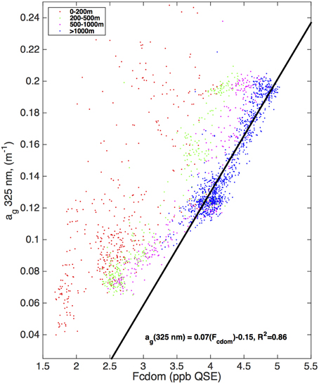
Figure 4. Scatter plot of CDOM absorption coefficient at 325 nm vs. F_cdom from the ECO fluorometer (ppb QSE) matching CDOM samples collected on the CLIVAR I8S/I9N section in the Indian Ocean Feb–Apr 2007. Samples are color coded by depth range (see legend). Regression line and correlation coefficient are shown for the samples collected at or below 1000 m depth along the transect line.

Nelson et al. (1998, 2010) have interpreted the absorption profile features as representing a balance between surface bleaching and water column production of UV-absorbing CDOM in the euphotic zone, with ventilation processes (e.g., subtropical or subantarctic mode water formation) affecting the profile between the euphotic zone and the main thermocline. The contrast seen with the fluorescence profile shows that for at least the subset of fluorescent CDOM that absorbs and fluoresces at the longest wavelengths, the production processes that affect UV-absorbing CDOM are absent or only weakly present.

Distribution of fluorescence EEM features (as represented by the A, T, M, and C regions of the EEM) also exhibited consistent patterns from basin to basin. Figure 5 shows vertical profiles of the fluorescence intensity for each region, divided up into different ocean regions based on latitude: North Atlantic (>40N), subtropical/tropical (40N–40S), Southern Ocean (40–55S), and Antarctic (south of 55S). In all regions the humic region A exhibited the highest fluorescence intensity. The humic A, M, and C regions were highly correlated to each other (R² > 0.92) and exhibited similar profiles, increasing from the surface into the main thermocline and remaining roughly constant into the abyssal. In all profiles the humic region C had higher fluorescence intensity than the humic region M.

FIGURE 5

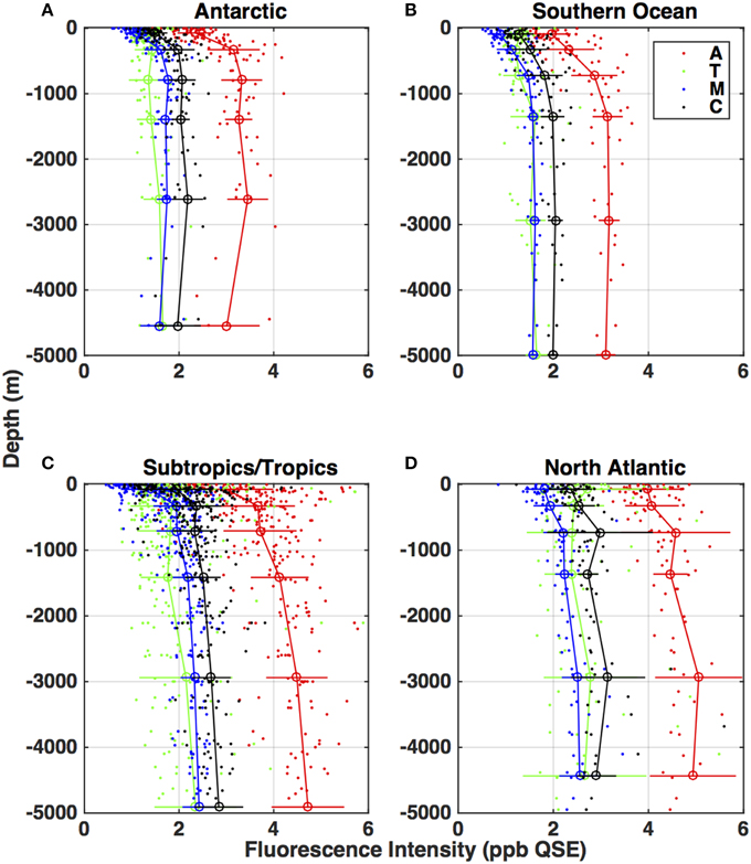
Figure 5. Depth distributions of CDOM fluorescence (ppb QSE) in the characteristic EEM regions (as denoted in Figure 2), for four latitude-bounded regions of the global ocean: (A) North Atlantic (>40 N), (B) subtropical/tropical regions of all oceans (40N–40S), (C) Southern Ocean (40S–55S), (D) Antarctic (below 55S). Red symbols: region A. Green symbols: region T. Black symbols: region C. Blue symbols: region M. Small dots are the individual measurements, connected circles with error bars are means and standard deviations for depth ranges 0–200, 200–500, 500–1000, 1000–2000, 2000–4000, and greater than 4000 m. The depth given for each mean value is the mean depth of the samples in the bin, so this varies slightly from panel to panel.

FIGURE 6

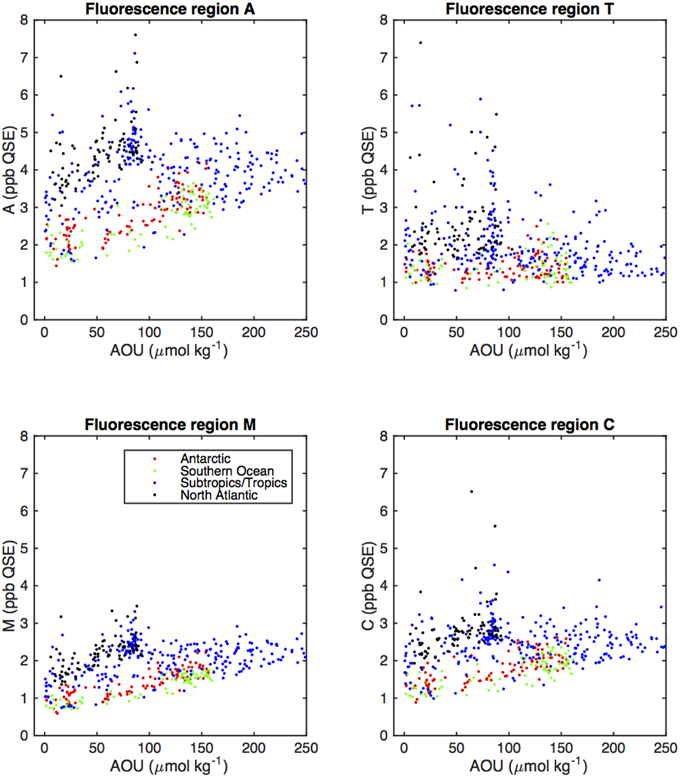
Figure 6. Scatter plots of fluorescent region intensities (Figure 2) vs. AOU (colors representing the different oceanic areas as defined in Figure 5).

The T fluorescence profiles exhibited more variability, but on average in each basin T region fluorescence intensity was higher in or near the euphotic zone (to 500 m), declined with depth into the intermediate waters (to 1000 m), and increased again in the main thermocline. T values were weakly correlated to the humic fluorescence regions (A, M, and C; R² < 0.43) because of the relatively large scatter in the T profiles and the differences between T and the humics in the top 500 m.

The North Atlantic samples (Figure 5A) exhibited on average the highest fluorescence in all regions, while the Southern Ocean (Figure 5C) and Antarctic (Figure 5D) samples had the lowest. The subtropical/tropical (Figure 5B) and North Atlantic humic fluorescence (A, M, and C) profiles were similar in magnitude below the thermocline but the North Atlantic sample fluorescence was higher at the surface.

The distribution of fluorescent components we report here is consistent with results of prior studies using fluorescence intensity (Chen and Bada, 1992; Determann et al., 1996; Yamashita and Tanoue, 2009), and in components derived from PARAFAC analysis of EEM components (Jørgensen et al., 2011; Catalá et al., 2015). The average increase in T values in the deep ocean we observed below the thermocline was not seen by Jørgensen et al. (2011) but is consistent with the long residence times of B-related components (adjacent to the T region) elucidated by Catalá et al. (2015).

We compared fluorescence intensities of the humic regions (A, M, and C) with AOU, which is for a given sample the difference between in situ oxygen concentration and the theoretical atmospheric equilibrated concentration of oxygen at in situ temperature, salinity, and pressure. Positive values of AOU in the ocean represent consumption of oxygen by the microbial community, and are closely linked to remineralization (Feely et al., 2004). Selected CDOM and FDOM components in the main thermocline have been seen as linearly related to AOU with high correlation (UV absorption, Nelson et al., 2010; and visible fluorescence components, Yamashita and Tanoue, 2008; Jørgensen et al., 2011), with the notable exception of the North Atlantic, where UV absorption or visible fluorescence components were much higher at low AOU (Nelson et al., 2010; Jørgensen et al., 2011). In the present study, correlation between fluorescence intensities in the canonical fluorescence regions and AOU varied between region and geographical area (Table 2).

TABLE 2

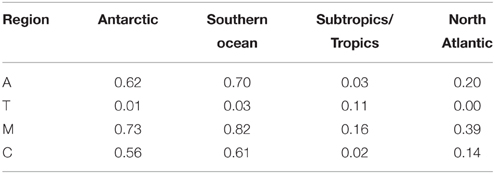
Table 2. Correlation coefficients (R²) for AOU (μmol kg⁻¹) vs. fluorescence region heights (ppb QSE) for the main fluorescence regions, divided into ocean basins (as in Figure 5).

UVA fluorescence in the T region was uncorrelated to AOU in all geographical regions.

Correlation between the visible (humic) fluorescence emission regions A and C and AOU was high in the Antarctic and Southern Ocean, but low in the North Atlantic and subtropics. Correlation between AOU and region M fluorescence was also higher in the North Atlantic. Low correlation between UVA fluorescence and AOU is consistent with previous results, and reflects the fact that higher values of T are generally found near the surface (Figure 5) and that UV absorption and the humic fluorescence regions increase as well as AOU in the main thermocline. The higher correlation we observed between M fluorescence and AOU in the North Atlantic is an exception to the general high correlation between A, C, and M fluorescence that we observed, and suggests differing dynamics between the components that give rise to A/C fluorescence and those that result in increases in M region fluorescence. The strongest correlations between fluorescent intensity and AOU in all basins were for the M region. This further suggests a link between remineralization and the formation of humic materials. Lack of correlation between T region fluorescence and AOU is most likely due to the more biolabile material represented by T fluorescence being remineralized in surface waters that are near to equilibrium with the atmosphere and thus have low and not consistently varying AOU.

We also compared fluorescence intensities in the different regions to the anthropogenic ventilation tracer CFC-12 (not shown). Correlations between the fluorescence intensity in the A, M, and C regions and CFC-12 were negative, indicating increasing humic material with increasing time since ventilation. As with AOU, fluorescence intensities in the T region were not correlated to CFC-12.

Analysis of Fluorescence Spectra Variability

We chose to use EOF analysis rather than the analogous and more commonly used parallel factors analysis (PARAFAC, Stedmon et al., 2003) to analyze the variance in fluorescence EEM data. Both EOF and PARAFAC methods decompose variability in three dimensional data sets (multiple EEMs) into two dimensional patterns and corresponding scalars that represent the contribution of each pattern to each sample. These analysis techniques allow for elucidation of variability patterns that are not immediately obvious from the fluorescence intensity data, such as assessment of the contributing factors to the M region, which includes both autochthonous and allochthonous components (Murphy et al., 2008), and for correlations between spectral regions that are not immediately apparent from inspecting the data.

The PARAFAC approach has been used successfully to discriminate between terrestrial and autochthonous CDOM fractions (Murphy et al., 2008), and to quantify characteristic components of EEM fluorescence that can be related to environmental variables, such as salinity, AOU, or amino acid concentration (Jørgensen et al., 2011). Typical PARAFAC implementations have modes which are exclusively positive values, so they better reflect components making up the EEM and their distribution. In the present study we are interested in the possibility of identifying transformations between components of the fluorescent material, so the ability of the EOF approach to have positive and negative regions in the modes is important.

For this data set, we identified three modes that each contributed more than 1% of the total variance (Figure 7), which we have designated EOF 1 (84.48%), EOF 2 (12.87%), and EOF 3 (1.57%). We have highlighted the nominal location of the main fluorescent regions (A, T, C, M) and the WETLabs fluorometer range (W). Distribution of the amplitudes for each mode is shown in Figure 8 as depth profiles (regions and depth averaging bins as in Figure 5).

FIGURE 7

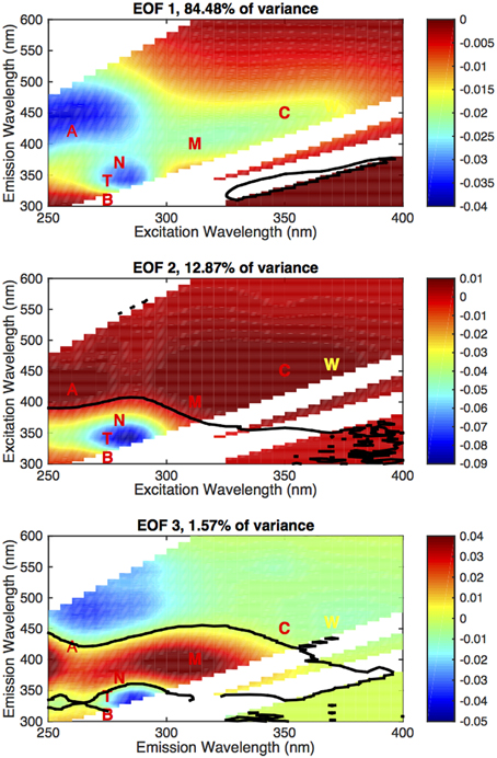
Figure 7. EOF basis functions (non-dimensional) computed from the EOF data, first three modes (annotated with nominal region locations and the F_cdom wavelength pair). The solid black line denotes where the EOF mode is zero. As in Figure 2, the white areas are masks where Rayleigh and Raman scattering obscure the sample fluorescence and are disregarded. The zero contour is interpolated when passing through this area and should not be considered significant.

FIGURE 8

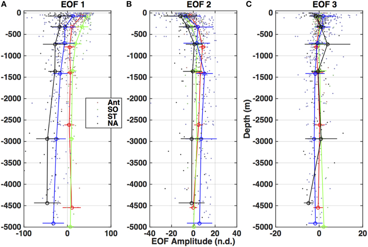
Figure 8. Depth profiles of the amplitudes for each of the three EOF modes (Figure 7) divided by basin (as in Figure 5). (A) Amplitude of EOF 1. (B) Amplitude of EOF 2. (C) Amplitude of EOF 3.

The first and dominant mode, EOF 1, exhibits all the features of the EEM (A, T/N, C, and M regions are identifiable, as in Figure 2C) and is below zero in the entire mode (Figure 7A), indicating a below-the-average contribution to the EEM when the corresponding amplitude is positive. The amplitude for this mode also covered the largest range of values and on average displayed two distinct profile patterns. In the subtropics and tropics and in the North Atlantic (Figure 8A), the amplitudes were strongly negative in the deep ocean (indicating a strong contribution of the inverse of this mode to the EEM), and increased steadily to the surface, where the average was slightly negative in the North Atlantic and slightly positive in the tropics and subtropics. In the Southern Ocean and the Antarctic, the Mode 1 amplitude was positive in the deep ocean and increased by a factor of ~8 from the main thermocline to the surface. This pattern reflects the differences in overall fluorescence intensity, or abundance of fluorescent material, in the global ocean.

The secondary modes, EOF 2 and EOF 3, both exhibited strong negative and positive areas (Figures 7B,C). EOF 2 (12.9% of the variance) features a strong negative peak in the UVA fluorescence region near the T and N locations, with positive peaks in the A and C regions (Figure 7B). The profiles of the amplitude of EOF 2 (Figure 8) increased in each ocean basin from below zero to zero or positive values near the top of the main thermocline (750–1000 m), then declined to near zero with increasing depth in the deep ocean. Increasing amplitudes of EOF 2 indicate a decreasing contribution of UVA fluorescence and an increase in the contribution of the humic fluorescence regions with depth from the euphotic zone to the mesopelagic.

EOF 3 (1.6% of the variance) has a distribution with a strong negative in UVA fluorescence and a strong positive near the M region (Figure 7C). The average profile of the EOF 3 amplitude showed slightly positive values near the euphotic zone (Figures 8A,C,D) or upper mesopelagic (Figure 8B), but was very close to zero in the deep ocean. This distribution suggests removal of UVA fluorescence balanced by increases in M fluorescence occurring in the euphotic zone and the upper mesopelagic.

EEM variability patterns in the first two EOF modes also exhibited correlation to indices of remineralization. Figure 9 shows scatter plots of AOU (μmol kg⁻¹) vs. EOF amplitude, color-coded by ocean basin. The first EOF mode (Figure 9A) shows a slight negative linear correlation with AOU, with the North Atlantic standing out as having a higher contribution from EOF 1 than the trend. The second EOF mode shows a strong correlation to AOU (Figure 9B) and the third EOF shows no correlation with AOU (Figure 9C), because on average positive values of EOF 3 occur only near the surface where AOU values are near zero (Figure 8). Similar results were obtained for correlations between EOF amplitudes and other indices of remineralization such as total CO₂ and inorganic nutrients (not shown). As with fluorescence intensities (Table 2), correlation of the EOF amplitudes with AOU varied by basin (Table 3). Correlations between AOU and EOF 1 and 2 amplitudes, were lowest in the North Atlantic and highest in the Antarctic and Southern Ocean areas. Similar lack of correlation was observed for EOF 1 in the subtropics and tropics (Table 3).

FIGURE 9

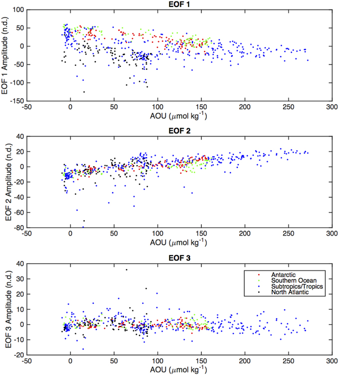
Figure 9. Scatter plots of EOF amplitudes (corresponding to EOF modes shown in Figure 7) vs. AOU (colors representing the different oceanic areas as in Figures 5, 6).

TABLE 3

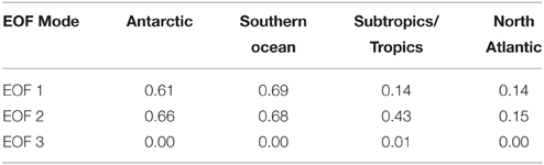
Table 3. Correlation coefficients (R²) between AOU and the amplitudes of the first three EOF modes, with regions defined as in Table 2.

The amplitude of EOFs 1 and 2 were also correlated to CFC-12 concentration (Table 4). Water of increasing ventilation age as assessed by CFC-12 concentration has been linked to increased CDOM UV absorption and decreased spectral slope in the North Atlantic interior (Nelson et al., 2007). The amplitude of EOF 1 showed a positive linear relationship with CFC-12 concentration in all basins. The amplitude of EOF 2 showed a negative linear relationship with CFC-12 that was significant in all basins except for the North Atlantic. This result qualitatively indicates that water of increasing ventilation age has an increased relative contribution of humic material and a decreased contribution of the humification process described by EOF 2. The lack of correlation between EOF 2 and CFC-12 in the North Atlantic is driven by a number of outliers of very low EOF 2 amplitude (not shown) at intermediate CFC-12 concentrations.

TABLE 4

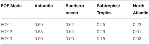
Table 4. Correlation coefficients (R²) between CFC-12 concentration and the amplitudes of the first three EOF modes, with regions defined as in Table 2.

Discussion

Characterization of Chromophoric DOM

Our results highlight the divergence between assessments of chromophoric DOM using absorption and fluorescence techniques. Comparative profiles of UV absorption and visible fluorescence (Figure 3) indicate that UV absorption represents a combination of UV absorbing and fluorescent material that originates in or near the euphotic zone (Nelson et al., 1998, 2010; Jørgensen et al., 2011; Yamashita et al., 2015), but also reflects the abundance of humic material in the main thermocline and deep ocean (Figure 4). This result further implies a diversity of chromophores in the DOM profile that can be further characterized using fluorescence EEM analysis. It is important to note that single-channel CDOM fluorometers only respond to a portion of potential fluorescent material in the ocean, and the data should be interpreted accordingly (e.g., Yamashita et al., 2015). In the case of the WETLabs ECO CDOM fluorometer, the fluorescence channel chosen responds to visible fluorescence near the C region, meaning it can be used to assess some forms of humic material but not the UVA fluorescing material found in freshly produced chromophoric DOM. Comparison of single channel visible fluorescence data with absorption data or EEM data can furnish insight into the location of remineralization processes that can increase CDOM abundance in the environment.

We attempted to use the absorption spectrum slope ratio parameter (Helms et al., 2008) to relate properties of the CDOM absorption spectrum to fluorescence properties and environmental variables. Slope ratio values in all ocean basins (not shown) ranged from 0.25 to 4 (n.d.) and exhibited a clear average depth profile with the highest values at the surface, and a deep ocean average of about 1.5, with considerable scatter. No relationships were found between the slope ratio and fluorescence region heights, nor were there correlations with the three main EOF amplitudes. We find that the slope ratio relates to increasing solar bleaching (high values) and increasing contribution of humic material (gradient to low values), as was postulated by Helms et al. (2008), but it does not directly relate to the presence or dynamics of fluorescent components.

Our results are largely consistent with the interpretation of fluorescent EEMs as reflecting a limited number of independent components (Stedmon and Nelson, 2015). In our results, the UVA fluorescing regions (T, B, and N) and the visible fluorescing regions (A, C, and M) were highly correlated to each other and only weakly correlated between groups. Nevertheless, we found some differences in the distribution of fluorescent components that suggest some diversity in processes controlling fluorescent materials, as we discuss below.

Origin and Dynamics of Humic Material in the Global Ocean

We interpret the patterns of fluorescence variability revealed by the EOF analysis as revealing transformation processes common to the whole ocean. The dominant mode of variability (EOF 1, Figure 7A) contains elements of all the fluorescence features of the EEM (cf. Figure 2) and we interpret the amplitude of EOF 1 as an overall index of fluorescent material abundance, as controlled by terrestrial material abundance or autochthonous production (increasing negative amplitude), and removal via bleaching (increasing positive amplitude). The profiles of EOF 1 amplitude differ significantly between the North Atlantic and subtropics (Figures 8A,B) and the Southern Ocean and Antarctic (Figures 8C,D). All profiles reflect the increasing contribution of EOF 1 with depth, but the North Atlantic and (sub)tropical profiles start at a higher level. The similarity between North Atlantic and subtropical/tropical profiles further suggests that the higher contribution of terrestrial material to the DOM found in the North Atlantic (Jørgensen et al., 2011; Catalá et al., 2015) is transported rapidly into the lower latitudes via meridional overturning circulation (Nelson et al., 2007).

EOF modes 2 and 3 appear to reveal removal of fresh DOM and production of humic material, as reflected in depth profiles (EOF 2 and 3, Figure 8) and correlation with AOU (EOF 2, Figure 9). In both cases these processes appear to be located in the upper ocean, in or near the euphotic zone (EOF 3) and above and within the main thermocline (EOF 2). This result is consistent with our observations of the single-channel visible fluorescence profiles vs. UV absorption profiles (Figure 3), which diverge above the main thermocline. The amplitude of EOF 2 is correlated to AOU and CFC-12, suggesting a connection to remineralization processes that occur over a significant length of time. The amplitude of EOF 3 is not correlated to AOU, but this is probably because this process appears to occur in the ventilated surface waters where AOU remains near zero.

The amount of variability contained in these remineralization-linked modes is small (<15%), implying that the primary source of gradients in fluorescent DOM in the global ocean is not autochthonous input of new fluorophores. Instead the distribution of fluorescence appears to be related to the removal of allochthonous fluorescent DOM by solar bleaching at the surface. This interpretation explains the higher CDOM/FDOM to AOU relationships observed in the North Atlantic (Nelson et al., 2010; Jørgensen et al., 2011) as being driven by high terrestrial preformed chromophoric DOM entering from the Arctic via the surface and North Atlantic Deep Water formation (Hernes and Benner, 1996; Granskog et al., 2012), and being removed at the surface via upwelling processes and solar bleaching (Nelson et al., 2010). In this interpretation the strong link between UV absorption, certain fluorescent components, and AOU (Nelson et al., 2010; Jørgensen et al., 2011) is partially coincidental. Increase of AOU is related to microbial consumption of POC and semi-labile DOC in the main thermocline, but the gradient in CDOM and FDOM in the main thermocline is essentially driven by removal in the upper ocean and supply of autochthonous CDOM from the thermohaline circulation.

These results are nevertheless consistent with the results of Catalá et al. (2015), who computed long (>350 years) lifetimes for fluorescent components in the deep ocean, which is longer than the oceanic turnover time. The difference between the ocean turnover time and the lifetimes of the fluorescent components is explained by the slow addition of new fluorescent material that we identify here. Our results indicate that these processes occur near the ocean surface and the main thermocline.

The processes that result in the patterns revealed by EOF 2 and 3 can include transformation of DOM, or removal of fresh DOM and production of humic DOM from colorless DOM and/or particles, as is implied by the microbial carbon pump hypothesis (Jiao et al., 2011). The general pattern of DOC distribution in the ocean (Hansell, 2002; Hansell and Carlson, 2015) suggests that the labile/semi-labile DOM is being remineralized, and it's possible some of this is transformed into humic material (Ogawa et al., 2001; Murphy et al., 2008). It is likely that remineralization of particles results in humic material formation, with perhaps “fresh” DOM as an intermediate step. Zooplankton excretia contain DOM that has distinct absorption spectra that do not resemble the canonical CDOM absorption spectra (Steinberg et al., 2004). Furthermore, the difference in the two EOF modes implies there is more than one process that converts “fresh” fluorescent DOM into two kinds of long-lived “humic” fluorescent DOM. Interestingly, in contrast to previous similar studies, we found that the average amount of fluorescence in the T region also increases slightly in the thermocline to the deep ocean (Figure 5). The increased T region fluorescence could represent newly produced UVA absorbing or fluorescing CDOM from microbial or heterotrophic processes (Nelson et al., 2004; Steinberg et al., 2004; Stedmon and Markager, 2005; Shimotori et al., 2009; Suksomjit et al., 2009) or material directly released via particle dissociation related to zooplankton grazing (Urban-Rich et al., 1996). This process could also be one source of UVA fluorescence in surface waters. The minimum in the T fluorescence profile can be explained by the processes described by EOFs 2 and 3 removing materials related to the T fluorescence and replacing them with humic materials.

As stated above, the results from the EOF analysis imply the presence of processes that convert fresh, UVA absorbing/fluorescing DOM into long-lived humic-like CDOM. These processes result in the apparent transfer of fluorescence from the T, B, and N region (where aromatic amino acids fluoresce) to the humic A and C regions (EOF 2) or the humic M region (EOF 3). One candidate for the sort of reaction that could underlie this process is a peptide-catalyzed aldol condensation reaction (Dziedzic et al., 2006) which is thought to give rise to visible-light absorbing oligomers that resemble humic material in marine aerosols (Nozière et al., 2007). There is also a photochemical condensation mechanism that can give rise to compounds with fulvic and humic acid-like absorption and fluorescence (Bianco et al., 2014; Gonsior et al., 2014), and the production of a visible light absorbing substance in the presence of nitrate was observed by Swan et al. (2012) in photochemical bleaching experiments. These processes are essentially abiotic, which is not consistent with the idea that the humification process is directly linked to remineralization. However, it is also likely, given the connections to AOU, that there are microbially mediated processes that perform similar functions that remain to be identified (Jørgensen et al., 2014). Aerosols as a source of new humic material to the global surface ocean should be considered as well, but solar bleaching is likely to give the material a short lifetime.

In summary, we conducted a global scale survey of chromophoric DOM in the ocean away from immediate terrestrial influence that included absorption and fluorescence properties. Our results partitioned chromophoric DOM into freshly created, UVA-absorbing-and-fluorescing material in the surface ocean, and long-lived, humic-like, visible-fluorescing material in the deep ocean. The main variability in humic material in the open ocean interior appears to result from introduction of allochthonous CDOM via the North Atlantic Deep Water, and removal of CDOM via solar bleaching of upwelled material. These results are consistent with previous global scale studies of fluorescent DOM (Jørgensen et al., 2011; Catalá et al., 2015). Furthermore, using EOF analysis of EEM data we identified two variability patterns that appear to reflect conversion of freshly produced material into humic material and localized these processes to the euphotic zone and the upper part of the main thermocline. Our results point to a need to identify the differences between terrestrial and marine humic materials and the reactions that “humify” DOM in the ocean.

Author Contributions

NN is the principal investigator and initiated the project. Both NN and JG contributed to the analysis, data processing, and quality control of the data. Both authors participated in writing the manuscript and interpreting the results.

Conflict of Interest Statement

The authors declare that the research was conducted in the absence of any commercial or financial relationships that could be construed as a potential conflict of interest.

Acknowledgments

This research was supported by grants from NASA (grants NAG5-13277 and NNX14AG24G) and NSF (OCE-0241614 and OCE-0648541) to NN and D. A. Siegel. We would like to acknowledge the ongoing support of the U.S. CO₂/CLIVAR/GO-SHIP Repeat Hydrography Program (Dick Feely, Lynne Talley, Rik Wanninkhof, Rana Fine), and the crews and support staff of the research vessels Revelle, Ronald H. Brown, Melville, and Nathaniel B. Palmer. Aimee Neeley, Stan Hooker, and Joaquin Chaves of NASA GSFC, collected samples for us on the I6S and S4P sections. Chantal Swan, Jamie Creason, Erica Aguilera, and Michelle Higgins conducted spectroscopic analysis in our lab, and our field teams included Dave Menzies, Chantal Swan, Ellie Halewood, Meg Murphy, KG Fairbarn, Erik Stassinos, and Eli Aghassi. Thanks also to Teresa Catalá for helpful discussions on EEM analysis and interpretation, and two anonymous reviewers for comments on the manuscript.

References

Andrew, A., Blough, N. V., Subramaniam, A., and Del Vecchio, R. (2013). Chromophoric dissolved organic matter (CDOM) in the Equatorial Atlantic Ocean: optical properties and their relation to CDOM structure and source. Mar. Chem. 148, 33–43. doi: 10.1016/j.marchem.2012.11.001

CrossRef Full Text | Google Scholar

Arístegui, J., Duarte, C. M., Agustí, S., Doval, M., Álvarez-Salgado, X. A., and Hansell, D. A. (2002). Dissolved organic carbon support of respiration in the dark ocean. Science 298:1967. doi: 10.1126/science.1076746

PubMed Abstract | CrossRef Full Text | Google Scholar

Bianco, A., Minella, M., De Laurentiis, E., Maurino, V., Minero, C., and Vione, D. (2014). Photochemical generation of photoactive compounds with fulvic-like and humic-like fluorescence in aqueous solution. Chemosphere 111, 529–536. doi: 10.1016/j.chemosphere.2014.04.035

PubMed Abstract | CrossRef Full Text | Google Scholar

Carlson, C. A., and Hansell, D. A. (2015). “DOM sources, sinks, reactivity, and budgets,” in Biogeochemistry of Marine Dissolved Organic Matter, 2nd Edn, eds D. A. Hansell and C. A. Carlson (San Diego, CA, Academic Press), 66–127.

Catalá, T. S., Reche, I., Fuentes-Lema, A., Romera-Castillo, C., Nieto-Cid, M., Ortega-Retuerta, E., et al. (2015). Turnover time of fluorescent dissolved organic matter in the dark global ocean. Nat. Commun. 6:5986. doi: 10.1038/ncomms6986

PubMed Abstract | CrossRef Full Text | Google Scholar

Chen, R. F., and Bada, J. L. (1992). The fluorescence of dissolved organic matter in seawater. Mar. Chem. 37, 191–221.

Google Scholar

Coble, P. G. (1996). Characterization of marine and terrestrial DOM in seawater using excitation- emission matrix spectroscopy. Mar. Chem. 51, 325–346.

Google Scholar

Coble, P. G. (2007). Marine optical biogeochemistry: the chemistry of ocean color. Chem. Rev. 107, 402–418. doi: 10.1021/cr050350+

PubMed Abstract | CrossRef Full Text | Google Scholar

Del Vecchio, R., and Blough, N. V. (2004). On the origin of the optical properties of humic substances. Environ. Sci. Technol. 38, 3885–3891. doi: 10.1021/es049912h

PubMed Abstract | CrossRef Full Text | Google Scholar

Determann, S., Reuter, R., and Wilkomm, R. (1996). Fluorescent matter in the eastern Atlantic Ocean.2. Vertical profiles and relation to water masses. Deep Sea Res. I 43, 345–360.

Google Scholar

Dziedzic, P., Zou, W., Háfren, J., and Córdova, A. (2006). The small peptide-catalyzed direct asymmetric aldol reaction in water. Org. Biomol. Chem. 4, 38–40. doi: 10.1039/B515880J

CrossRef Full Text

Feely, R. A., Sabine, C., Schlitzer, R., Bullister, J. L., Mecking, S., and Greeley, D. (2004). Oxygen utilization and organic carbon remineralization in the upper water column of the Pacific Ocean. J. Oceanogr. 60, 45–52. doi: 10.1023/B:JOCE.0000038317.01279.aa

CrossRef Full Text | Google Scholar

Feely, R. A., Talley, L. D., Johnson, G. C., Sabine, C. L., and Wanninkhof, R. (2005). Repeat hydrography cruises reveal chemical changes in the North Atlantic. EOS Trans. Am. Geophys. Union 86, 404–405. doi: 10.1029/2005EO420003

CrossRef Full Text

Gonsior, M., Hertkorn, N., Conte, M. H., Cooper, W. J., Bastviken, D., Druffel, E., et al. (2014). Photochemical production of polyols arising from significant photo-transformation of dissolved organic matter in the oligotrophic surface ocean. Mar. Chem. 163, 10–18. doi: 10.1016/j.marchem.2014.04.002

CrossRef Full Text | Google Scholar

Granskog, M. A., Stedmon, C. A., Dodd, P. A., Amon, R. M. W., Pavlov, A. K., de Steur, L., et al. (2012). Characteristics of colored dissolved organic matter (CDOM) in the Arctic outflow in the Fram Strait: assessing the changes and fate of terrigenous CDOM in the Arctic Ocean. J. Geophys. Res. 117, C12021. doi: 10.1029/2012JC008075

CrossRef Full Text | Google Scholar

Green, N. W., Perdue, E. M., Aiken, G. R., Butler, K. D., Chen, H., Dittmar, T., et al. (2014). An intercomparison of three methods for the large-scale isolation of oceanic dissolved organic matter. Mar. Chem. 161, 14–19. doi: 10.1016/j.marchem.2014.01.012

CrossRef Full Text | Google Scholar

Hansell, D. A. (2002). “DOC in the global ocean carbon cycle,” in Biogeochemistry of Marine Dissolved Organic Matter, eds D. A. Hansell and C. A. Carlson (San Diego, CA: Academic Press), 685–715.

Google Scholar

Hansell, D. A. (2013). Recalcitrant dissolved organic carbon fractions. Annu. Rev. Mar. Sci. 5, 421–445. doi: 10.1146/annurev-marine-120710-100757

PubMed Abstract | CrossRef Full Text | Google Scholar

Hansell, D. A., and Carlson, C. A. (2015). Biogeochemistry of Marine Dissolved Organic Matter, 2nd Edn. San Diego, CA, Academic Press.

Google Scholar

Helms, J. R., Stubbins, A., Ritchie, J. C., Minor, E. C., Kieber, D. J., and Mopper, K. (2008). Absorption spectral slopes and slope ratios as indicators of molecular weight, source, and photobleaching of chromophoric dissolved organic matter. Limnol. Oceanogr. 53, 955–969. doi: 10.4319/lo.2008.53.3.0955

CrossRef Full Text | Google Scholar

Hernes, P. J., and Benner, R. (1996). Terrigenous organic matter sources and reactivity in the North Atlantic Ocean and a comparison to the Arctic and Pacific oceans. Mar. Chem. 100, 66–79.

Google Scholar

Jaffe, R., McKnight, D., Maie, N., Cory, R., McDowell, W. H., and Campbell, J. L. (2008). Spatial and temporal variations in DOM composition in ecosystems: the importance of long-term monitoring of optical properties. J. Geophys. Res. 113:G04032. doi: 10.1029/2008JG000683

CrossRef Full Text | Google Scholar

Jiao, N., Azam, F., and Sanders, S. (eds.). (2011). Microbial Carbon Pump in the Ocean. Washington, DC: AAAS.

Google Scholar

Jørgensen, L., Stedmon, C. A., Granskog, M. A., and Middelboe, M. (2014). Tracing the long-term microbial production of recalcitrant fluorescent dissolved organic matter in seawater. Geophys. Res. Lett. 41, 2481–2488. doi: 10.1002/2014GL059428

CrossRef Full Text | Google Scholar

Jørgensen, L., Stedmon, C. A., Tragh, T., Markager, S., Middleboe, M., and Sondergaard, M. (2011). Global trends in the fluorescence characteristics and distribution of marine dissolved organic matter. Mar. Chem. 126, 139–148. doi: 10.1016/j.marchem.2011.05.002

CrossRef Full Text | Google Scholar

Lonborg, C., Yokokawa, T., Herndl, G. J., and Alvarez-Salgado, X. A. (2015). Production and degradation of fluorescent dissolved organic matter in surface waters of the eastern north Atlantic ocean. Deep Sea Res. I 96, 28–37. doi: 10.1016/j.dsr.2014.11.001

CrossRef Full Text | Google Scholar

Maritorena, S., Siegel, D. A., and Peterson, A. R. (2002). Optimization of a semianalytical ocean color model for global-scale applications. Appl. Optics 41, 2705–2714. doi: 10.1364/AO.41.002705

PubMed Abstract | CrossRef Full Text | Google Scholar

Miller, R. L., Belz, M., Del Castillo, C., and Trzaska, R. (2002). Determining CDOM absorption spectra in diverse coastal environments using a multiple pathlength, liquid core waveguide system. Continental Shelf Res. 22, 1301–1310. doi: 10.1016/S0278-4343(02)00009-2

CrossRef Full Text | Google Scholar

Murphy, K. R., Stedmon, C. A., Waite, T. D., and Ruiz, G. M. (2008). Distinguishing between terrestrial and autochthonous organic matter sources in marine environments using fluorescence spectroscopy. Mar. Chem. 108, 40–58. doi: 10.1016/j.marchem.2007.10.003

CrossRef Full Text | Google Scholar

Nelson, N. B., Carlson, C. A., and Steinberg, D. K. (2004). Production of chromophoric dissolved organic matter by Sargasso Sea microbes. Mar. Chem. 89, 273–287. doi: 10.1016/j.marchem.2004.02.017

CrossRef Full Text | Google Scholar

Nelson, N. B., and Coble, P. G. (2010). “Optical analysis of chromophoric dissolved organic matter,” in Practical Guidelines for the Analysis of Seawater, ed O. Wurl (Boca Raton, FL: CRC), 79–96.

Nelson, N. B., and Siegel, D. A. (2013). The global distribution and dynamics of chromophoric dissolved organic matter. Annu. Rev. Mar. Sci. 5, 447–476. doi: 10.1146/annurev-marine-120710-100751

PubMed Abstract | CrossRef Full Text | Google Scholar

Nelson, N. B., Siegel, D. A., Carlson, C. A., and Swan, C. M. (2010). Tracing global biogeochemical cycles and meridional overturning circulation using chromophoric dissolved organic matter, Geophys. Res. Lett. 37, L03610. doi: 10.1029/2009GL042325

CrossRef Full Text | Google Scholar

Nelson, N. B., Siegel, D. A., Carlson, C. A., Swan, C., Smethie, W. M. Jr., and Khatiwala, S. (2007). Hydrography of chromophoric dissolved organic matter in the North Atlantic. Deep Sea Res. I 54, 710–731. doi: 10.1016/j.dsr.2007.02.006

CrossRef Full Text | Google Scholar

Nelson, N. B., Siegel, D. A., and Michaels, A. F. (1998). Seasonal dynamics of colored dissolved material in the Sargasso Sea. Deep Sea Res. I 45, 931–957.

Google Scholar

Nieto-Cid, M., Aìlvarez-Salgado, X. A., and Peìrez, F. F. (2006). Microbial and photochemical reactivity of fluorescent dissolved organic matter in a coastal upwelling system. Limnol. Oceanogr. 51, 1391–1400. doi: 10.4319/lo.2006.51.3.1391

CrossRef Full Text | Google Scholar

Nozière, B., Dziezdic, P., and Cordova, A. (2007). Formation of secondary light-absorbing “fulvic-like” oligomers: a common process in aqueous and ionic atmospheric particles? Geophys. Res. Lett. 34, L21812, doi: 10.1029/2007gl031300

CrossRef Full Text | Google Scholar

Ogawa, H., Amagai, Y., Koike, I., Kaiser, K., and Benner, R. (2001). Production of refractory DOC by bacteria. Science 292, 917–920. doi: 10.1126/science.1057627

PubMed Abstract | CrossRef Full Text

Preisendorfer, R. W., and Mobley, C. D. (1988). Principal Component Analysis in Meteorology and Oceanography. San Diego, CA: Elsevier.

Google Scholar

Rochelle-Newall, E. J., and Fisher, T. R. (2002). Production of chromophoric dissolved organic matter ?uorescence in marine and estuarine environments: an investigation into the role of phytoplankton. Mar. Chem. 77, 7–21. doi: 10.1016/S0304-4203(01)00072-X

CrossRef Full Text | Google Scholar

Schlitzer, R. (2008). Ocean Data View. Available online at: http://odv.awi.de/

Shimotori, K., Omori, Y., and Hama, T. (2009). Bacterial production of marine humic-like fluorescent dissolved organic matter and its biogeochemical importance. Aquat. Microb. Ecol. 58, 55–66. doi: 10.3354/ame01350

CrossRef Full Text | Google Scholar

Siegel, D. A., Maritorena, S., Nelson, N. B., Hansell, D. A., and Lorenzi-Kayser, M. (2002). Global distribution and dynamics of colored dissolved and detrital organic materials. J. Geophys. Res. 107, 3228. doi: 10.1029/2001jc000965

CrossRef Full Text | Google Scholar

Stedmon, C. A., and Markager, S. (2001). The optics of chromophoric dissolved organic matter (CDOM) in the Greenland Sea: An algorithm for differentiation between marine and terrestrially derived organic matter. Limnol. Oceanogr. 46, 2087–2093. doi: 10.4319/lo.2001.46.8.2087

CrossRef Full Text | Google Scholar

Stedmon, C. A., and Markager, S. (2005). Tracing the production and degradation of autochthonous fractions of dissolved organic matter by fluorescence analysis. Limnol. Oceanogr. 50, 1415–1426. doi: 10.4319/lo.2005.50.5.1415

CrossRef Full Text | Google Scholar

Stedmon, C. A., Markager, S., and Bro, R. (2003). Tracing dissolved organic matter in aquatic environments using a new approach to fluorescence spectroscopy. Mar. Chem. 82, 239–254. doi: 10.1016/S0304-4203(03)00072-0

CrossRef Full Text | Google Scholar

Stedmon, C. A., and Nelson, N. B. (2015). “The optical properties of DOM in the ocean,” in Biogeochemistry of Marine Dissolved Organic Matter, 2nd Edn, eds D. A. Hansell and C. A. Carlson (San Diego, CA, Academic Press), 481–508.

Steinberg, D. K., Nelson, N., Carlson, C. A., and Prusak, A. C. (2004). Production of chromophoric dissolved organic matter (CDOM) in the open ocean by zooplankton and the colonial cyanobacterium Trichodesmium spp. Mar. Ecol. Prog. Ser. 267, 45–56. doi: 10.1016/j.dsr.2012.01.008

CrossRef Full Text | Google Scholar

Suksomjit, M., Nagao, S., Ichimi, K., Yamada, T., and Tada, K. (2009). Variation of dissolved organic matter and fluorescence characteristics before, during and after Phytoplankton Bloom. J. Oceanogr. 65, 835–846. doi: 10.1007/s10872-009-0069-x

CrossRef Full Text | Google Scholar

Swan, C. M., Nelson, N. B., and Siegel, D. A. (2012). The effect of surface irradiance on the absorption spectrum of chromophoric dissolved organic matter in the global ocean. Deep Sea Res. I 63, 52–64. doi: 10.1016/j.dsr.2012.01.008

CrossRef Full Text | Google Scholar

Swan, C. M., Siegel, D. A., Nelson, N. B., Carlson, C. A., and Nasir, E. (2009). Biogeochemical and hydrographic controls on chromophoric dissolved organic matter in the Pacific Ocean. Deep Sea Res. I 56, 2172–2192. doi: 10.1016/j.dsr.2009.09.002

CrossRef Full Text | Google Scholar

Urban-Rich, J., McCarty, J. T., Fernandez, D., and Acuna, J. L. (1996)., Larvaceans and copepods excrete fluorescent dissolved organic matter (FDOM). J. Exp. Mar. Biol. Ecol. 332, 96–105.

Google Scholar

Yamashita, Y., Lu, C.-J., Ogawa, H., Nishioka, J., Obata, H., and Saito, H. (2015). Application of an in situ fluorometer to determine the distribution of fluorescent organic matter in the open ocean. Mar. Chem. 177, 298–305. doi: 10.1016/j.marchem.2015.06.025

CrossRef Full Text | Google Scholar

Yamashita, Y., and Tanoue, E. (2003). Chemical characterization of protein-like fluorophores in DOM in relation to aromatic amino acids. Mar. Chem. 82, 255–271. doi: 10.1016/S0304-4203(03)00073-2

CrossRef Full Text | Google Scholar

Yamashita, Y., and Tanoue, E. (2008). Production of bio-refractory fluorescent dissolved organic matter in the ocean interior. Nat. Geosci. 1, 579–582. doi: 10.1038/ngeo279

CrossRef Full Text | Google Scholar

Yamashita, Y., and Tanoue, E. (2009). Basin scale distribution of chromophoric dissolved organic matter in the Pacific Ocean. Limnol. Oceanogr. 54, 598–609. doi: 10.4319/lo.2009.54.2.0598

CrossRef Full Text | Google Scholar

Zepp, R., Sheldon, W. M., and Moran, M. A. (2004). Dissolved organic fluorophores in southeastern US coastal waters: correction method for eliminating Rayleigh and Raleigh scattering peaks in excitation – emission matrices. Mar. Chem. 89, 15–36. doi: 10.1016/j.marchem.2004.02.006

CrossRef Full Text | Google Scholar