Optical Proxies for Terrestrial Dissolved Organic Matter in Estuaries and Coastal Waters

Introduction

Terrestrial organic carbon (OC) flux from rivers and estuaries into coastal oceans is on the order of 0.2 Pg C yr⁻¹ and constitutes a major part of the oceanic carbon cycle (Raymond and Spencer, 2014). Absorbing and fluorescing properties of chromophoric dissolved organic matter (CDOM) have been used to fingerprint OC sources, and often to track terrestrial DOM fluxes into the ocean (Coble, 2007). These optical properties can be used as proxies for organic matter in such instances to calibrate remote sensing observations from space and in deployed on in situ platforms (Mannino et al., 2008; Fichot and Benner, 2011; Etheridge et al., 2014). In particular, ultraviolet (UV) absorption has been used to quantify DOC and measure its quality (sources) (Ferrari, 2000; Stedmon et al., 2000; Helms et al., 2008; Fichot and Benner, 2011; Asmala et al., 2012).

Studies on terrestrial DOC fluxes from rivers into coastal waters rely on strong correlations between DOC and lignin (e.g., Hernes and Benner, 2003; Spencer et al., 2008; Walker et al., 2009; Fichot and Benner, 2012). In terms of estuarine and coastal ocean biogeochemistry, this work has mainly been restricted to large rivers and to delta front estuaries (Raymond and Spencer, 2014). Both CDOM and lignin have been studied widely in estuaries separately, but rarely together (e.g., Osburn and Stedmon, 2011). This paucity of information complicates an understanding of how estuarine processes modify terrestrial DOC during transport to coastal waters.

In this work, we report on an analysis of CDOM, DOC, and lignin measurements from six estuaries across North America: the Atchafalaya River, the Mackenzie River, the Chesapeake Bay, Charleston Harbor, Puget Sound, and the Neuse River Estuary (Figure 1). These six systems represent a wide variety of estuaries in terms of their formation, morphology, hydrology, and their geographical distributions, as well as their catchment vegetation and land use. The aim of this work is to determine efficacy of using CDOM properties to predict DOC and lignin concentration across these six estuaries. Both CDOM absorption and excitation-emission matrix (EEM) fluorescence, modeled by parallel factor analysis (PARAFAC), were evaluated. Finally, we assessed whether optical-chemical linkages that underlie coupled optics-biogeochemical models can be applied widely across different estuarine types.

FIGURE 1

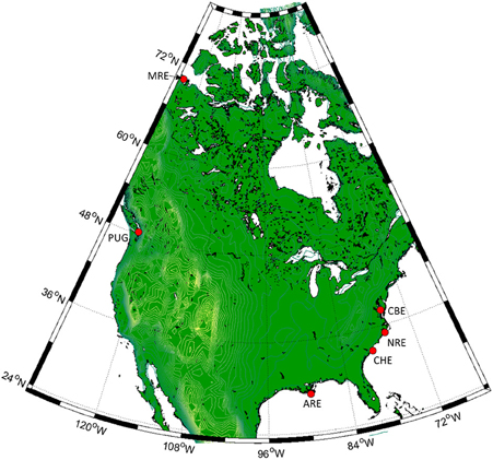
Figure 1. Locations of the six North American estuaries in this study. Clockwise from right: Chesapeake Bay (CBE), Neuse River (NRE), Charleston Harbor (CHE), Atchafalaya River (ARE), Puget Sound (PUG), and Mackenzie River (MRE).

Methods

Study Sites

Six North American estuarine and coastal systems were sampled from 2003 to 2011 (Table 1, Figure 1; station coordinates, Table S1). The Atchafalaya River Estuary (ARE) is a component of the Mississippi-Atchafalaya River System (MARS) a major component of the Gulf of Mexico. This river receives diverted flow from the Mississippi River and thus reflects the Mississippi's drainage. The Chesapeake Bay (CBE) is the largest estuary in the continental United States and the largest system we studied. The CBE has multiple river inputs and is heavily impacted by urban and agricultural land use. Charleston Harbor (CBE) is a coastal plain estuary dominated by three main river inputs (Ashley, Cooper, and Wando). The Mackenzie River (MRE) is one of the largest rivers flowing into the Arctic Ocean and drains boreal forest and Arctic tundra. The Neuse River Estuary (NRE) drains into the largest lagoonal estuary in the United States, the Pamlico Sound. The NRE receives drainage from the lower Piedmont to Coastal Plain and, like CBE, has had chronic problems with eutrophication. Puget Sound in the Pacific Northwest region of the United States contains several deep fjords (e.g., Hood Canal) and several small rivers. In this study, we includes samples from Hood Canal, the Snohomish River, and the Straits of Juan de Fuca, the latter which connect Puget Sound to the Pacific Ocean. Thus, our data set cover estuaries sampled across wide geographic and climatic regions.

TABLE 1

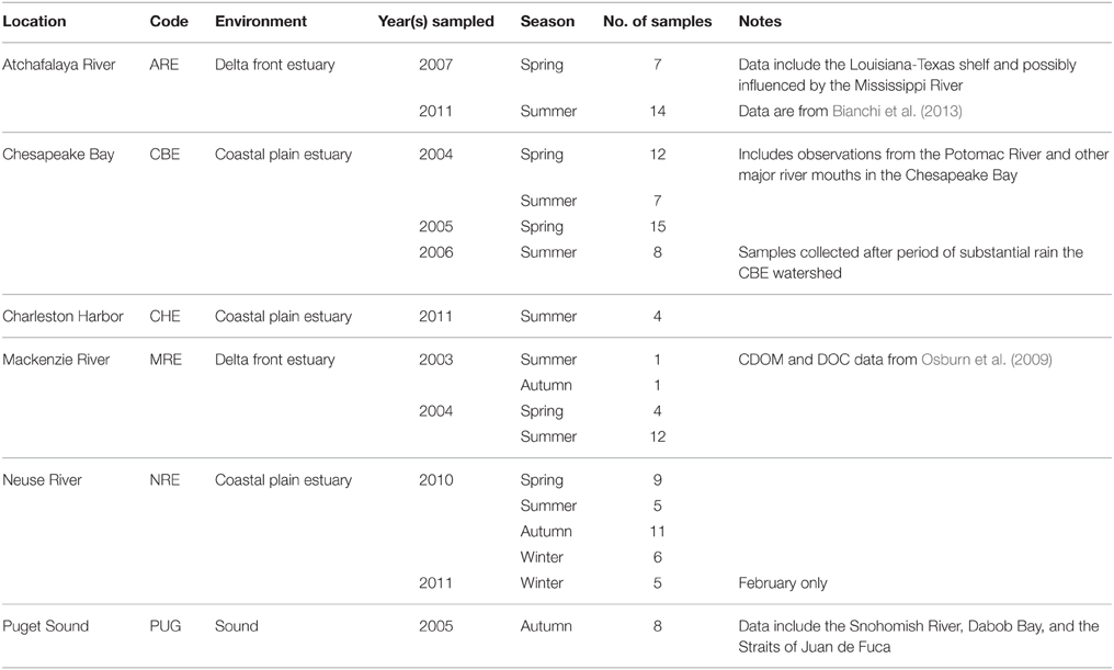
Table 1. Site description information for the estuaries and coastal waters in this study.

There were more observations for the CBE and NRE than the other systems. Most observations came from estuarine environments although several samples came from coastal waters across the continental shelf (with the exception of Puget Sound). These seasonal samplings spanned a salinity range from 0 to 36. Thus, the data set represents a range of river influences from weak (Puget Sound) to strong (Atchafalaya and Neuse River Estuaries) and hence captures most hydrologic conditions encountered in estuaries. Only the NRE had a truly comprehensive seasonal dataset covering spring, summer, autumn, and winter. Most samples were collected from just below the water surface, though some were collected at mid-depths either by pneumatic pumps with Teflon tubing suspended at depth or by Niskin bottles. Salinity was often different for these sub-surface samples compared to their surface water counterparts so these samples were treated separately.

Two events of note for these samplings are important to mention. In July 2006, the Chesapeake Bay was sampled roughly 1 week after a period of intense summer squalls with increased freshwater discharge to the Bay. Discharge of the Bay's main tributary, the Susquehanna River, measured at Conowigo, MD, approached 11,000 m³ s⁻¹ (USGS gauge 01578310) and the Potomac River, measured near Washington, DC, approached 2300 m³ s⁻¹ (USGS gauge 01646502). Mean annual flows for each river (2000-2014) were 1184 and 346 m³ s⁻¹, respectively.

The second event occurred in the Atchafalaya River basin whereby a flooding event in May 2011 required that the Morganza Floodway near Baton Rouge, be opened for the first time in 40 years, to prevent New Orleans from being flooded. More specifically, the floodway was opened on May 14, 2011 when the Mississippi River reached a flow of over 42,000 m³s⁻¹, the highest flow recorded since floods of 1927.

Optical Analyses

Absorbance and fluorescence were measured according to Osburn et al. (2009, 2012). Briefly, samples were filtered shipboard, refrigerated and analyzed within 3 weeks of each field effort. Absorbance (A) was measured on filtered samples, although two different filter sizes were used: 0.2 μm filters prior to 2009 and 0.7 μm filters after 2009. All samples were scanned from 200 to 800 nm against air and periodic MilliQ water blanks were scanned and subtracted from sample spectra. Samples were diluted if the absorbance in a 1-cm cell was greater than 0.4 at 240 nm. Absorbances at wavelength, λ, corrected for MilliQ water blanks were converted to Napierian absorption coefficients (a):

$\begin{array}{cc}a(\lambda )=\frac{A({\lambda }_{sample})-A({\lambda }_{blank})}{L}\times 2.303& (1)\end{array}$

This study focused on absorption at 350 nm (a₃₅₀) to quantify CDOM absorption in comparison with previous work (Uher et al., 2001; Hernes and Benner, 2003; Lønborg et al., 2010; Spencer et al., 2013).

Two different fluorometers were used: a Shimadzu RFPC-5301 (samples before 2009) and a Varian Eclipse (samples after 2009). The time lag between their usages precluded intercalibration of their results, though the similarity in response to analyzing the same standards or to Raman unit scaling has been reported (Cory et al., 2010). However, data treatment for each instrument was the same. Standard corrections for lamp excitation and detector emission were applied, and afterward, corrections for the inner filter effects were applied. Scanning was performed with an excitation ranging from 250 to 450 nm (by 5 nm) and emission ranging from 300 to 600 by at 1 nm resolution. Integration time on the RFPC-5301 instrument was 0.2 s (e.g., Boyd and Osburn, 2004). On the Varian instrument, scanning was performed with an excitation range from 240 to 450 nm in 5 nm increments and an emission range of 300 – 600 nm in 2 nm increments. Integration time on the Varian instrument was 0.125 s (Osburn et al., 2012). Shimadzu fluorescence results were resized in Matlab to match with Varian results over the excitation and emission wavelength ranges. Finally, the results were calibrated first to the water Raman signal of each instrument and then in quinine sulfate units (QSU). All fluorescence data were normalized to the total integrated fluorescence in each EEM prior to PARAFAC (Murphy et al., 2013).

DOC Analysis

Dissolved organic carbon (DOC) and δ¹³C-DOC values were measured using wet chemical oxidation coupled with isotope ratio mass spectrometry (Osburn and St-Jean, 2007). Samples were acidified with 85% H₃PO₄ in the field (if not frozen) and stored in the dark until analysis. Samples were pre-sparged with ultrapure helium to remove inorganic carbon prior to analysis. WCO-IRMS system was calibrated daily with IAEA standards of glutamic acid, sucrose, oxalic acid, and caffeine. Routine analysis of the University of Miami Deep Sea Reference DOC (DSR) for this methodology produced DOC concentrations of 45 ± 3 μM and δ¹³C-DOC values of −20.5±0.4‰ (N = 11 for samples before 2008 and N = 32 for samples after 2008). Error on DOC concentrations by this method were <3% and reproducibility on δ¹³C-DOC values was ±0.4‰.

Dissolved Lignin Analysis

Lignin was extracted from DOM via passage over C₁₈ cartridges that were either assembled in the laboratory or purchased pre-assembled (Mega Bond Elut cartridges) (Louchouarn et al., 2000; Kaiser and Benner, 2011). Samples were eluted from C₁₈ cartridges with methanol, dried and oxidized to release lignin-derived phenols into solution. Microwave oxidation was used for all samples following Goñi and Montgomery (2000), except ARE samples from 2011, which used oven oxidation (Bianchi et al., 2013). Samples were then acidified, recovery standards added, then extracted into ethyl acetate and dried prior to storage at 4°C. Prior to analysis, samples were re-dissolved into pyridine, derivatized with BSTFA+1% TMS, and then measured via gas chromatography-mass spectrometry. Calibration curves of 8 lignin derived phenols (vanillin, acetovanillone, vanillic acid, syringealdehyde, acetosyringone, syringic acid, p-coumaric acid, and ferulic acid) were used to quantify concentrations. Detailed methods for lignin analysis can be found in Osburn and Stedmon (2011), Bianchi et al. (2013), and Dixon (2014).

Statistical Analyses

Parallel factor analysis (PARAFAC) was conducted on EEMs from all estuaries in this study using the DOMFluor toolbox for Matlab (Mathworks, Natick MA) (Stedmon and Bro, 2008). Matlab statistical toolbox (releases spanning 2003 to present) was also used for other statistical tests. R²-values are adjusted values and significance of regression models was tested at α = 0.05. Principle components analysis (PCA) was conducted using the PLS_Toolbox (Eigenvector, Inc., Seattle, WA) for Matlab. Autoscaling was used on variables measured prior to PCA.

Results

Summary Statistics for Each System

CDOM, DOC, lignin, and (when available) δ¹³C-DOC data for each system are summarized as boxplots (Figure 2) and presented in its entirety (Table S1). Note that δ¹³C-DOC values were not available for ARE in summer 2011, and for some CHE and NRE samples. Mean CDOM absorption at 350 nm (a₃₅₀) was highest for NRE (13.03 m⁻¹) and lowest for Puget Sound (0.90 m⁻¹). The CBE and CHE estuaries had a₃₅₀ values between 2 and 3 m⁻¹ and the ARE and MRE estuaries had a₃₅₀ values between 3 and 5 m⁻¹ (Figure 2A). Mean DOC concentration for the NRE was 680 μM whereas for the other estuaries DOC averaged ca. 250 μM (Figure 2B). PUG DOC values were overall the lowest of the data set and averaged 90 μM. The NRE also had the highest lignin concentration among the estuaries studied, with a mean Σ8 of 24.2 μg L⁻¹, while PUG again had the lowest amount of lignin (mean Σ₈ = 0.8 μg L⁻¹) (Figure 2C). The mean Σ₈ concentrations for CBE, CHE, ARE, and MRE ranged from 3.5 to 4.3 μg L⁻¹. Both the CBE and NRE had more observations than other systems, especially CHE and PUG.

FIGURE 2

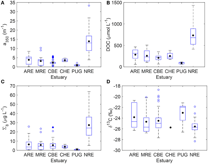
Figure 2. Boxplots summarizing key variables measured for the six estuaries in this study. (A) CDOM absorption at 350 nm (a₃₅₀); (B) DOC concentration; (C) sum of 8 lignin phenols (Σ₈); (D) stable carbon isotope values of DOC (δ¹³C-DOC). The blue solid line is the median and the black circle is the mean; the edges of the boxes denote the 25th and 75th percentiles, while the whiskers denote the 10th and 90th percentiles, and blue circles represent outliers.

Stable carbon isotope values exhibited ranges common to estuarine environments and representing mixtures of terrestrial and planktonic organic matter (Figure 2D). Typically, riverine dissolved organic matter (DOM) values ranges from −26 to −28‰. By contrast, marine phytoplankton δ¹³C values typically range from −22 to −18‰, reflecting different carbon fixation sources than land plants. Median δ¹³C-DOC value was −24.7±2.1‰ which is typical of estuarine DOC (Bauer, 1997; Bianchi, 2007). Median δ¹³C-DOC values for MRE and CBE were −24.7 and −24.5‰, respectively—close to median of the entire data set. Median δ¹³C-DOC values for ARE and PUG were enriched at −23.8‰ and −23.0‰ respectively, suggesting more planktonic inputs. CHE only had one observation of δ¹³C-DOM (−25.8‰). NRE had δ¹³C-DOC values that were slightly depleted relative to the median at −25.4‰. Further, this system exhibited the largest range of δ¹³C-DOC values (−22 to −28‰) with the most frequent value of −26‰.

Trends with Salinity

If coastal mixing between two end members (e.g., river and ocean) is conservative, chemical constituent concentrations plotted against salinity will exhibit a linear relationship. Deviations from conservative linear mixing are then interpreted to indicate biogeochemical cycling, for example, production or consumption of a chemical constituent or optical property. We examined trends in concentration of CDOM, DOC, and lignin against salinity for our entire dataset, considering this simple mixing scenario. For the most part, linear trends with salinity were found, even for multiple river inputs in systems such as CBE (Figure 3). NRE had the lowest salinity range (0–20) but also the largest seasonal variability probably due to the higher resolution of sampling.

FIGURE 3

Figure 3. Trends in (A) a₃₅₀, (B) DOC concentration, and (C) sum of 8 lignin-derived phenols (Σ₈) with salinity. Colors denote the individual points from the six estuaries studied. Neuse River estuary (NRE) samples are plotted on the right axis of each figure.

Relationships Between CDOM Absorbance and Fluorescence

Many studies of CDOM and lignin have used a₃₅₀ to quantify CDOM absorption, so this convention was used for the remainder of the study with the understanding that primary CDOM absorption is caused by conjugated systems such as aromatic rings which have peak absorption near 254 nm (Weishaar et al., 2003; Del Vecchio and Blough, 2004). We chose a₃₅₀ following on the work of Ferrari (2000) and Hernes and Benner (2003)—some of the first reported CDOM-DOC and CDOM-lignin relationships for coastal waters (Baltic Sea and Mississippi River plume, respectively). CDOM concentrations at a₂₅₄ and a₃₅₀ were highly correlated (R² = 0.96; P < 0.0001; N = 130).

The PARAFAC model we fit to our entire dataset produced four validated components, three of which exhibited humic-like fluorescence (C1–C3) and one which was amino acid-like (C4) (Figures 4A–D). Spectra for these components are presented along with results of the split-half validation (Figure S1). These components were matched against the OpenFluor database for similarity with up to 75 PARAFAC models from a range of aquatic ecosystems including boreal lakes, small and large rivers, estuaries, coastal, and open ocean water. Component 1 (C1) had excitation (Ex) maxima of 260 and 345 nm and emission (Em) maximum of 476 nm (Figure 4A). This component closely resembles soil-derived fulvic acids (Senesi, 1990). C2 had Ex/Em maxima of 310/394 nm and this component has been surmised as originating from microbial humic substances (Coble, 1996) (Figure 4B). C3 had Ex/Em of 250/436 nm and resembles humic substances (Figure 4C). C4 had Ex/Em of 275/312 nm which is situated between the fluorescence maxima of tyrosine and tryptophan, both of which are prevalent in natural waters (Wolfbeis, 1985; Figure 4D).

FIGURE 4

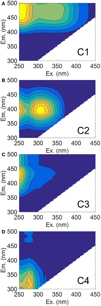
Figure 4. EEM contour plots of the four PARAFAC components matched against the OpenFluor database. (A) C1 (soil fulvic acid); (B) C2 (microbial humic); (C) C3 (terrestrial humic); and (D) C4 (protein-like).

Of interest in this study were matches to our model components of those in river, estuaries, and coastal waters. Criteria for matching components were set at 95% similarity and assessed through Tucker's Congruence Coefficient via the OpenFluor database. Matches of each component with components from models in the database are also provided (Table S2). The maximum fluorescence intensity (FMax) values for C1 were most strongly corrected to a₃₅₀ values over the entire dataset (R² = 0.89; P < 0.001). A stepwise multiple linear regression (MLR) was used to explore the importance of other components in explaining variation of a₃₅₀ (data not shown). C2 was highly correlated to C1, while C3 only improved the model by <1%, which suggested their removal from the regression equation. C4 was not significant (P = 0.126).

Relationships Between DOC and Lignin

DOC and lignin concentrations for the six estuaries showed a positive correlation (DOC = 17.05 ± 1.04 × Σ₈ + 175 ± 18; R² = 0.68; P < 0.001; N = 130) (Figure 5). Although linear, the R²-value of this relationship suggests that roughly 30% of DOC was not explained by lignin concentration. Seasonal variability in these estuaries, observed in plots of DOC or lignin vs. salinity (Figures 3A–C), was evident in relationships between DOC and lignin for four estuaries where there were observations during more than one season (Table 2). Linear regressions for spring samplings in ARE and MRE produced correlation coefficients, R², >0.9. By contrast, CBE and NRE had much weaker correlations: R² = 0.57–0.84 for CBE and R² = 0.61 for NRE. CBE in particular showed seasonal variability represented as three regression lines for each of 2004, 2005, and 2006 were fit to the data and had much higher correlation coefficients than did the fit to all 3 years (R² = 0.35). For NRE, a linear fit to all values produced a correlation coefficient similar to CBE (R² = 0.29). DOC values >900 μM were excluded from NRE and the regression analysis re-ran, producing a much better fit (R² = 0.61; Table 2).

FIGURE 5

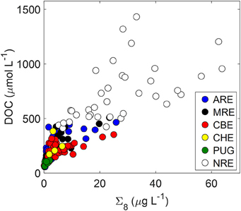
Figure 5. Relationship between DOC and lignin (Σ₈) concentrations for the six estuaries in this study.

TABLE 2

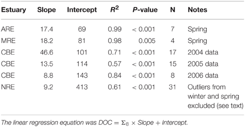
Table 2. Linear regression results between lignin concentration (Σ₈) and DOC concentration for four estuaries in this study.

Discussion

Predicting DOC and Lignin Concentrations in Estuaries and Coastal Waters Using CDOM

The major aim of this study was to determine the extent to which a cross-system optical-biogeochemical model for DOM could be developed for hydrologically-variable estuaries. We anticipated that the variability of estuarine ecosystems would complicate the robustness of one simple model to describe DOC or lignin concentrations across a gradient of estuaries and adjacent coastal waters. Using simple linear regression, we found that CDOM concentration measured at 350 nm explained greater than 70% of the variance both in DOC and dissolved lignin concentrations (Figures 6A,B). The higher correlation coefficient for the CDOM-lignin model than the CDOM-DOC model suggested that CDOM is generally terrestrial in many different estuaries. Results from the Mississippi River plume and boreal estuaries support this suggestion (e.g., Hernes and Benner, 2003; Asmala et al., 2012).

FIGURE 6

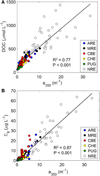
Figure 6. Relationships between CDOM and (A) DOC (DOC = 40 ± 2 × a₃₅₀ + 138 ± 16) and (B) lignin (Σ₈ = 2.03 ± 0.07 × a₃₅₀ + −0.27 ± 0.59), linking the optics and chemistry of DOM. Regression lines are shown along with correlation coefficients for the regression.

In fact, a₃₅₀ serves as an excellent optical proxy for DOC for many estuaries as seen for North American rivers (Spencer et al., 2012). In that study, the authors showed consistent patterns of strong linear trends between a₂₅₄ and DOC and a₃₅₀ and DOC (see their Figure 5). That result was consistent with the linear relationship between a₃₅₀ and DOC found for the estuaries in this study (R² = 0.77; P < 0.001; N = 130). Regression of DOC on a₂₅₄ values produced similar results (R² = 0.76; P < 0.001; N = 130). Thus, it appears that general trends between optics and chemistry can be modeled with some certainty.

CDOM absorption at a₃₅₀ also was an excellent proxy for lignin for the six estuaries we studied (R² = 0.87; Figure 6B). Using a₃₅₀, Hernes and Benner (2003) found higher R²-values (0.98) for the Mississippi River plume, but their model was only for one sampling in May 2000. Fichot and Benner (2012) found positive linear relationships for lignin vs. a₃₅₀ for the Mississippi River Plume in all seasons over 2009-2010 (R²-values ranged from 0.89 to 0.99) and noted a seasonality in the slope coefficients for these relationships.

Intercepts of these types of regressions should be interpreted with some caution (Stedmon and Nelson, 2014). For the CDOM-DOC relationship, the y-intercept value (139 μM DOC) was significantly different from zero (P < 0.001). This would suggest that non-CDOM DOC in these estuaries approximates 140 μM but one must be careful in that these regressions are sensitive to seasonality and hydrology (see below discussion on seasonal and episodic variability). While Fichot and Benner found robust CDOM-DOC and CDOM-lignin models for the Mississippi River plume, variability in regression statistics for CDOM-DOC models in Finnish boreal estuaries led to the suggestion that regional or sub-system models might be necessary (Asmala et The latter study's results were consistent with the findings for the North American estuaries in this study.

Fluorescence Indicated Dominant Influence of Terrestrial Sources of CDOM in Estuaries and Coastal Waters

Although CDOM absorption was a strong predictor for DOC and lignin, PARAFAC of EEM fluorescence provides a powerful means of characterizing DOC sources and prior work has shown good correspondence between fluorescence and lignin (Amon et al., 2003; Walker et al., 2009; Osburn and Stedmon, 2011) but also has identified planktonic fractions (Zhang et al., 2009; Romera-Castillo et al., 2011; Osburn et al., 2012). For example, a fluorescence component similar to our C3 was found to be important for predicting terrestrial DOM flux from the Baltic Sea though (Osburn and Stedmon, 2011). Combining that component with a protein-like component similar to our C4, those authors estimated terrestrial DOC flux from the Baltic Sea using multiple linear regression (MLR). Recently, Osburn et al. (2015) applied the same fluorescence-based approach to modeling DOM dynamics in a small tidal creek system and found very strong relationships between fluorescence and DOM (R² > 0.9). Thus, we were interested in determining how this PARAFAC model, based on six estuaries (but weighted toward the CBE and NRE in terms of the numbers of samples), would perform with respect to identifying markers for terrestrial DOC (as lignin) and for planktonic DOC (as amino-acid like fluorescence, Osburn and Stedmon, 2011).

For this determination, stepwise MLR was run in a forward mode in which only positive coefficients with P < 0.05 were allowed to enter the model. The rationale was that to be predictive, fluorescence signals should have a positive relationships with lignin or with DOC. For lignin, we found that FMax values for C1 predicted about 82% of variability in Σ₈ values (Σ₈ = −1.18+2.048 × FMaxC1; P < 0.001; n = 130). The intercept was not significant. C2 had a negative coefficient and was excluded which is sensible because this component matched with microbial humic substances. C3 was not significant in the model and C4 only increased the variance explained by about 1%. Therefore, C1 served as our terrestrial DOM marker.

C1 matched with 7 models on the OpenFluor database—all suggestive of terrestrial humic substances. This component's longwave emission properties (e.g., >450 nm) likely result from highly conjugated aromatic material and resemble isolated fulvic acids from soils and sediments (Senesi, 1990). C4 shared spectral features with 8 models on the OpenFluor database from estuarine and marine environments and, in each case, this component was attributed to protein-like or amino acid-like fluorescence. However, using partial least squares regression, Hernes et al. (2009) was able to demonstrate that fluorescence centered as Ex/Em wavelengths near our C4 was best predictive of lignin concentration. That result was not surprising given that lignin phenols originate as the fluorescent aromatic amino acid phenylalanine (Goodwin and Mercer, 1972), but does indicate the care that must be taken in calibrating fluorescence signals for prediction of chemical quantities. With this consideration in mind, we next attempted stepwise MLR to use FMax values from the PARAFAC model to predict DOC concentrations in these estuaries.

MLR produced the following model:

$\begin{array}{cc}\begin{array}{l}\text{DOC}=82.05\times \text{FMaxC1}-112.53\times \text{FMaxC2}+\text{11}.\text{99}\times \\ \text{ FMaxC3}+38.88\times \text{FMaxC4}+163.70\end{array}& (2)\end{array}$

FMax values for all components were significant in the model (P < 0.001). C1 explained the most variance. The coefficient for C2 was negative, which meant that as C2 fluorescence increased, DOC concentration decreased. This result suggested consumption of DOC by bacteria, and is consistent with the removal of terrestrial DOC in estuaries by bacteria (Moran et al., 2000; Raymond and Bauer, 2000; McCallister et al., 2004). C3 and C4, while significant, were less important in terms of their explanatory power in the model. Thus, as expected, the strongest linkage between optics and chemistry in the DOM of these six estuaries of this study was due to terrestrial organic matter. Overall, the MLR model demonstrated the importance of terrestrial organic matter as a dominant component of the DOC in these estuaries.

However, none of our four PARAFAC components matched to the Osburn and Stedmon (2011) model components which underscores the uncertainty in using fluorescence and provides a clear example of the considerations needed when using this approach. Universal models of fluorescence as a means to quantify DOC sources are likely unattainable because fluorescence properties are sensitive to biogeochemistry. For example, photodegradation is well known to cause proportionally more loss of fluorescence at longer excitation and emission wavelengths that arise from the conjugation and aromaticity that typify terrestrial CDOM sources (Boyle et al., 2009; Gonsior et al., 2009). Biodegradation, independently and in conjunction with photodegradation, can also cause a variety of spectral changes to fluorescence (Miller and Moran, 1997; Boyd and Osburn, 2004; Stedmon and Markager, 2005). Given the dynamics within and among estuaries, it is not surprising that our fluorescence results performed less well on hydrologically-variable estuaries than did those of Osburn and Stedmon (2011) which focused on one estuarine system. It is thus recommended that PARAFAC be limited to local or perhaps regional modeling of estuarine DOM.

Geographic Variability in CDOM-Lignin Relationships for Estuaries and Coastal Waters

The above discussion suggested ways in which both CDOM absorption and fluorescence could be utilized to link optical and chemical properties of estuaries and coastal waters both in terms of quantification (absorption) and estimates of DOM sources (fluorescence). PCA was then utilized to explore the optical and chemical data of these six estuaries with respect to each other (Figure 7). Ratios of syringyl lignin to vanillyl phenols (S:V) and ratio of cinnamyl to vanillyl phenols (C:V) were included in this analysis to identify plant tissue sources. FMax values for C2 were removed from the analysis because of the high correlation with C1. A 2-component PCA model explained 70% of the variance in these data.

FIGURE 7

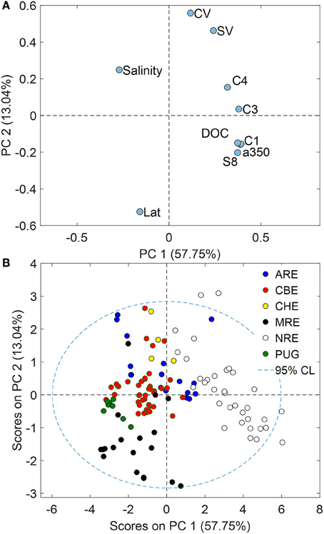
Figure 7. (A) Loadings plot for variables and (B) scores plots for samples resulting from a PCA of the optical and chemical data for the six estuaries studied. PC1 likely represented discharge while PC2 was linked to latitude.

Loadings for optical and chemical variables measured for these six estuaries showed interesting separation that supports the strong connection between CDOM and lignin in them (Figure 7A). Loadings for C1, a₃₅₀, DOC, and Σ₈ all clustered tightly in the lower right quadrant of the plot, closer to the PC1 axis than the PC2 axis and opposite of the loading for salinity. This result supports the concept that control of DOC and CDOM in these six estuaries was due to freshwater sources of terrestrial organic matter in rivers flowing into them. PC1 thus may be strongly tied to river flow; all CDOM, but especially C3, align with this axis.

Loadings for latitude and C:V and S:V ratios align most closely with PC2 and suggested some geographic influence on the DOM quality across these estuaries. Loadings for latitude were strongly negative on PC2 while loadings for S:V and C:V were strongly positive on PC2. This result was sensible because vegetation in lower latitudes typically has much more angiosperms than the gymnosperms that dominate boreal and Arctic environments. Lignin quality across broad geographic gradients typically is reflected in these ratios (Onstad et al., 2000; Amon et al., 2012).

Scores for our samples clearly support the trends with freshwater (PC1) and with latitude (PC2) (Figure 7B). Scores for NRE were most positive on PC1 and NRE was the most freshwater dominated estuary of those in this study, with the highest CDOM, DOC, and lignin concentrations. By contrast, MRE had the most negative scores on PC2, reflecting the dominance of lignin in NRE by conifers which are depleted in cinnamyl phenols and thus C:V ratios were near zero. Similarly, PUG scores were negative on PC2 representing the influence of mainly coniferous vegetation around the PUG and Snohomish River watersheds. However, CBE fell near the mean of the data set likely reflecting large vegetative and land use gradients in its watershed of this temperate estuary.

The PCA suggested PARAFAC provided little distinction between these estuaries, which was consistent with a recent study of Arctic rivers (Walker et al., 2013). However, C4 fluorescence was more closely related to plant tissue type as indicated by loadings FMax values for C4, S:V, and C:V ratios that were positive both on PC1 and PC2. This could indicate that these lower latitude estuaries have more angiosperm and non-woody tissue producing this signal (Hernes et al., 2007). For example, tidal pulsing exported higher molecular weight, more aromatic and CDOM-rich marsh-derived DOC to the Rhode River sub-estuary of CBE (Tzortziou et al., 2008). Therefore, we may expect that more lignin also was exported from the marshes adjacent to the estuaries we studied. Most of our study sites were in temperate climates dominated by Spartina marsh plants—angiosperm grasses which would be enriched both in syringyl (S) and cinnamyl (C) phenols relative to vanillyl (V) phenols. Alternatively, these lower-latitude systems might coincidentally be more productive than the higher latitude systems. For example, one caveat to our results suggesting C4 is correlated to plant tissue type is that an unequal number of observations were made across six different systems and data for these cross-system regressions were dominated by CBE and NRE—both meso- to eutrophic estuaries (Paerl et al., 2006).

Seasonal and Episodic Variability in Optical Proxies for DOM within Specific Estuary Types

Fichot and Benner (2012) have developed remarkably consistent models relating CDOM absorption to lignin phenol concentration in surface waters from a large delta front estuary system, the Mississippi-Atchafalaya River System (MARS), of which ARE is a component. They noted seasonal variability of DOM in freshwater end members of these large river systems, and attributed most of that to seasonal variability in discharge. Asmala et al. (2012) also found substantial variability in CDOM-DOC relationships for boreal estuaries. The MARS was similar to the MRE whereas the boreal estuaries were similar to the coastal plain-type estuaries, NRE and CBE.

The strongest control on CDOM and DOC in the estuaries we studied was river flow, which contributed CDOM-rich terrestrial DOM to these estuaries and their coastal waters. This was evident because of the linear relationship between CDOM and DOC and CDOM and lignin that we found across multiple estuary types (Figures 6A,B). For the CDOM-lignin relationship, the y-intercept value (−0.50 μg L⁻¹) was not significantly different from zero (P = 0.503). This result suggested that the vast majority of CDOM in these estuaries originated from terrestrial sources. CDOM absorption at wavelengths >300 nm is primarily due to conjugated molecules such as lignin (Del Vecchio and Blough, 2004). Therefore, it makes sense that in estuaries and coastal waters where rivers and coastal wetlands contribute DOM, this material will be highly conjugated and chromophoric (Raymond and Spencer, 2014).

Variable hydrologic regimes are well known to influence concentrations and relationships of CDOM, DOC and lignin in rivers and this certainly appears the case in many estuaries (Hernes et al., 2008; Saraceno et al., 2009; Spencer et al., 2010). For example, both CDOM and DOC doubled in concentration during the flushing hydroperiod of the tropical Epulu River (NE Congo) compared to the post-flush period, while Σ₈ values tripled (Spencer et al., 2010). Discharge values for the major rivers flowing into the MRE, ARE, NRE, and CBE are listed in Table S3.

We found corroborating evidence of hydrologic variability in optical-biogeochemical models within estuaries for ARE, MRE, CBE, and NRE that was seasonal and episodic (Figures 8A–H). We do not extend our analysis of relationships beyond linear regression models as Fichot and Benner (2012) have done for DOC-normalized results; rather, we focus on the basic CDOM, DOC, and lignin measurements that can be used in a first order optical algorithm for satellite retrievals of properties related to ocean color (Mannino et al., 2008; Tehrani et al., 2013). These are expressed as either DOC or Σ₈ as a function of a₃₅₀. Further, some concern about collinearity of the Fichot and Benner models has been raised (Asmala et al., 2012). Our subsequent analysis of seasonal trends exclude CHE and PUG for which we have too few observations.

FIGURE 8

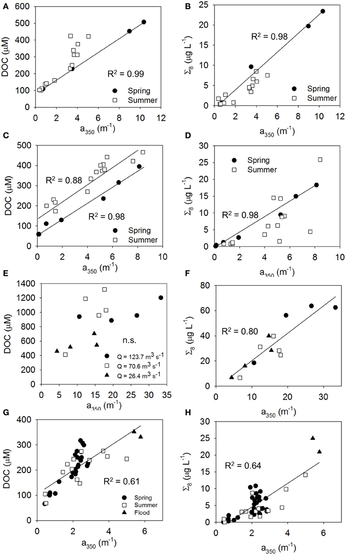
Figure 8. Relationships between CDOM and DOC (left column of panels A, C, E, and G) and lignin (right column of panels B, D, F, and H) linking the optics and chemistry of DOM, influenced by hydrologic variability. (A,B) MRE showing influence of spring freshet, (C,D) ARE showing influence of 2011 Mississippi River flood, (E,F) NRE showing seasonal influence of river discharge, and (G,H) CBE showing the influence of heavy rains in summer 2006. Significant linear regressions are shown while slope and intercept values and regression statistics are in Table 3. For (F–H), the regressions were fit to all of the data.

For MRE, spring and summer distinctions were clear in the relationships between CDOM and DOC or CDOM and lignin that coincided with the spring flush of freshwater from Arctic rivers (Table 3 and Table S3). For example, in MRE, far more CDOM, DOC, and lignin were found in June just after the freshet as opposed to late August when the river had returned to base flow (Figures 8A,B). This pattern is common of Arctic rivers which deliver the majority of DOM during the freshet (Amon et al., 2012). Larger concentrations of Σ₈ during spring indicates that this also is the case for ARE. Spring meltwaters in the upper Midwest US might similarly create a freshwater pulse leading to high discharge of the entire Mississippi-Atchafalaya system as suggested by the results of Fichot and Benner (2012). Therefore, in LDEs the large river flow forcing in these systems could exhibit seasonally predictable patterns.

TABLE 3

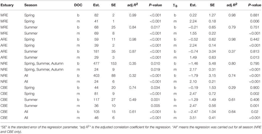
Table 3. Parameter estimates (Est.) for linear regression models (DOC or Σ₈ = m × a₃₅₀ + b).

In contrast to ARE and MRE, which are both large delta front estuaries that extend well into coastal waters, NRE is a smaller, microtidal system with a long residence time between 20 and 120 days (Pinckney et al., 1998). However, like ARE and MRE, NRE is heavily riverine influenced, though this estuary exhibited a 3-fold range in CDOM, DOC, and lignin concentrations at the freshwater end member (Figure 3; Table S1). Variability of the NRE data around the regression line describing the general CDOM-DOC relationship we found for the estuaries in this study was the greatest and suggested some change in either the source or quality of DOM entering the NRE annually (Figure 6A).

The influence of discharge on CDOM, DOC, and lignin patterns across the NRE was further investigated (Figures 9A–C). River discharge (Q) to the NRE at Ft. Barnwell, NC, (USGS Gauging Station 02091814) was averaged for the 7 days prior to the sampling date on which the observations were made (Table S3). It was clear that high river flow contributed more CDOM, DOC, and lignin into the NRE than at lower flow. At lower flows (Q = 26–70 m³ s⁻¹) CDOM decreased downstream but DOC and lignin were rather constant. This pattern changed substantially when Q = 123.7 m³ s⁻¹ at Ft. Barnwell and concentrations of CDOM in the NRE doubled whereas concentrations of DOC and lignin nearly tripled. Thus, it is not surprising that the NRE data, which were collected roughly monthly over a 12-month period, captured the variability in high and low flow regimes. The change in DOM quality was somewhat larger than the load of terrestrial DOM as evidenced by the higher R²-value of the CDOM-lignin relationship as opposed to the CDOM-DOC relationship (Figures 6A,B).

FIGURE 9

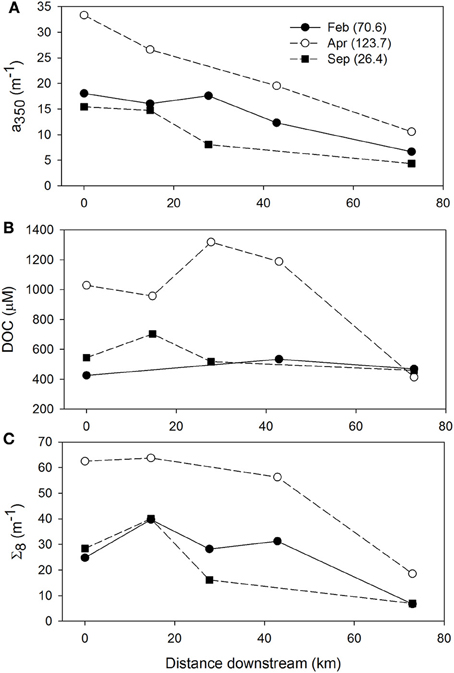
Figure 9. Within system variability of (A) CDOM absorption at a₃₅₀, (B) DOC concentration, and (C) lignin concentration for the meso-eutrophic Neuse River Estuary. Values in parentheses for each month are the mean discharge at Ft. Barnwell, NC (USGS Station 02091814) for the 7 days preceding the date of sampling.

In addition to seasonal variability, we had two examples of episodic loadings of terrestrial DOM into estuaries from high periods of rainfall that also contributed to deviations from general trends found in this study. In summer 2011, a flood in the Mississippi River basin delivered historically higher amounts of DOC to the coastal Gulf of Mexico (Bianchi et al., 2013). This resulted in large amounts of CDOM and lignin, as well (Figures 8C,D). Overall DOC concentrations were higher, illustrating how climatic events can perhaps increase the transfer of terrestrial DOC to coastal waters (Table 3). Other work in the northern Gulf of Mexico has shown that coastal marshes are a significant source of dissolved lignin to the estuaries and very shallow inner shelf regions (Bianchi et al., 2009), but not likely to the broader shelf areas (Fichot et al., 2014). Coastal marsh DOM could be mobilized as well during storm events. Large loads of terrestrial DOM have been shown to be delivered to the NRE by its watershed during tropical storms (Paerl et al., 1998; Osburn et al., 2012).

In June 2006, summer squalls produced heavy rainfall in the mid-Atlantic United States, leading to 6- to 10-fold higher river discharges to the CBE (Table S3). We had two observations each of CDOM, DOC, and lignin in the Potomac River, a sub-estuary of CBE, to provide a contrast of terrestrial DOM inputs between spring and summer (Figures 8G,H). These observations are titled “Flood” Figures 8G,H and demonstrate proportionally higher amounts of CDOM per unit DOC and lignin, respectively. These observations underscore the higher CDOM, DOC, and lignin values observed in the freshwater inputs to CBE (Figures 3A–C).

Finally, episodic variability in CDOM-DOC relationships for some estuaries could be linked to autotrophic sources of DOM within estuaries. NRE and CBE experience periodic, yet chronic, eutrophication caused by excessive nitrogen loading from their watersheds (Paerl et al., 2006; Paerl, 2009). Primary production from algae can add DOC to the estuary but not lignin. Phytoplankton-derived, and microbially-transformed, sources of CDOM have been documented for many estuaries and coastal waters though uncertainty in the magnitude of this source exists (Stedmon and Markager, 2005; Romera-Castillo et al., 2011; Osburn et al., 2012; Stedmon and Nelson, 2014). Spring and autumn blooms in NRE could explain why intercepts of seasonal regression models for DOC vs. a₃₅₀ were often larger than in summer and winter (Table 3; Pinckney et al., 1998). Estuarine systems in which long residence time allows for substantial primary production can add a planktonic component to the overall estuarine CDOM signal (Fellman et al., 2011; Osburn et al., 2012). Evidence of this phenomenon likely explains the NRE results which were the most variable of estuaries studied here. Intertidal production of DOC is probably low in this microtidal estuary, but was observed in the Gironde estuary, which also has internal production of CDOM, further complicating optical-biogeochemical models (Abril et al., 2002; Huguet et al., 2009). Together, for NRE, these effects caused a disruption of classic binary mixing between river and seawater that underlay the robust CDOM-DOC and CDOM-lignin relationships found by Fichot and Benner (2012) for the MARS.

Similar to NRE, the CBE exhibited large seasonal variability in CDOM-DOC and CDOM-lignin relationships. Direct evidence of phytoplankton production of CDOM in the Chesapeake Bay has been less well documented (Rochelle-Newall and Fisher, 2002). CBE also has multiple sub-estuaries flowing into it and rivers of these sub-estuaries have 50–80% more DOC than the Susquehanna River, which is the main tributary to CBE (Raymond and Bauer, 2000). Thus, it was not surprising that seasonal and interannual variability were also important to this estuary. We lacked sufficient observations from the Potomac River and York River estuaries, which comprise large amounts of flow to the lower CBE. A focus on these systems might improve the overall picture with respect to CDOM, DOC, and lignin dynamics in the CBE as well as parse out commonalities among eutrophic estuaries in contrast to LDEs.

Conclusions

This work has narrowed the knowledge gap between CDOM-DOC and CDOM-lignin relationships that have been developed for large rivers and coastal waters by focusing specifically on estuaries, which are notoriously heterogeneous. We found that both DOC and lignin can be quantified with CDOM absorption with roughly 75% certainty across several estuary types. CDOM fluorescence suggested that the dominant source of CDOM in the estuaries and coastal waters we studied was terrestrial inputs. Hydrologic variability in river flow appeared to be the dominant control on the linkage of CDOM and DOC we observed in these estuaries—and showed the major influence of terrestrial DOM. High river flow contributed more CDOM and lignin. Low river flow and longer residence time within the estuary allowed for planktonic contributions to DOM. Much of the variability in DOM quality likely is explained by the history of this material in the soil organic matter pool and any subsequent biogeochemical processing across the terrestrial-marine continuum (Marín-Spiotta et al., 2014).

It was beyond the scope of this study to compute yields of terrestrial (or planktonic) DOC from these estuaries, but the models developed may be scaled to remote sensing platforms in space and in situ observatories (e.g., Mannino et al., 2008; Etheridge et al., 2014; Osburn et al., 2015). Wide variability in the models among these estuaries thus suggested that local or regional models should be developed for prediction of terrestrial DOM fluxes into the coastal ocean using optical properties. A one size fits all approach is not appropriate for estuaries collectively, but possible for classes of estuaries (e.g., large delta front vs. coastal plain) (Asmala et al., 2012). Upscaling to remotely sensed observations are entirely possible yet must require optimization of basic equations based on calibration and validation data sets. Results from such work will continue to spur new questions, hopefully integrating other disciplines, such as meteorology and climatology, and ultimately leading to a greater understanding of organic matter sources and cycling in coastal waters.

Author Contributions

CO conceived of this manuscript, analyzed data, and lead the writing. TB provided data analysis, co-wrote, and assisted in data collection. MM and RC co-wrote and assisted in data collection. TB and HP contributed data and co-wrote.

Funding

The following agencies are thanked for their financial support: Strategic Environmental Research and Development Program, ER-1431 and ER-2124 (MM, CO); North Carolina Department of Environment and Natural Resources, Contracts #4443 and #5371 (HP, CO); and the Lower Neuse Basin Association (HP).

Conflict of Interest Statement

The authors declare that the research was conducted in the absence of any commercial or financial relationships that could be construed as a potential conflict of interest.

Acknowledgments

We thank the following people for technical support during the field and laboratory work done for this study: Tiffanee Donowick, Erin Kelley, Jeff Denzel, Mike Shields, Lauren Handsel, and Jennifer Dixon. Special thanks to Warwick Vincent for logistical support for the Mackenzie River Estuary sampling. We also thank the captains and crews of the following vessels that were used to assemble this data set: RV Cape Henlopen, RV John Sharp, RV Cape Hatteras, RV Barnes, CCGS Nahidik, and RV Pelican. The following agencies are thanked for their financial support: Office of Naval Research (CO, TB, RC), Strategic Environmental Research and Development Program (MM, CO), NASA (CO, TB), and National Science Foundation Ecosystems Studies Program project 1119704 (HP), and the NC Dept. of Environment and Natural Resources-Lower Neuse Basin Association (HP, CO).

Supplementary Material

The Supplementary Material for this article can be found online at: https://www.frontiersin.org/article/10.3389/fmars.2015.00127

References

Abril, G., Nogueira, M., Etcheber, H., Cabeçadas, G., Lemaire, E., and Brogueira, M. J. (2002). Behaviour of organic carbon in nine contrasting European estuaries. Estuar. Coast. Shelf Sci. 54, 241–262. doi: 10.1006/ecss.2001.0844

CrossRef Full Text | Google Scholar

Amon, R. M. W., Budéus, G., and Meon, B. (2003). Dissolved organic carbon distribution and origin in the Nordic Seas: exchanges with the Arctic Ocean and the North Atlantic. J. Geophys. Res. 108, 3221. doi: 10.1029/2002jc001594

CrossRef Full Text | Google Scholar

Amon, R. M. W., Rinehart, A. J., Duan, S., Louchouarn, P., Prokushkin, A., Guggenberger, G., et al. (2012). Dissolved organic matter sources in large Arctic rivers. Geochim. Cosmochim. Acta 94, 217–237. doi: 10.1016/j.gca.2012.07.015

CrossRef Full Text | Google Scholar

Asmala, E., Stedmon, C. A., and Thomas, D. N. (2012). Linking CDOM spectral absorption to dissolved organic carbon concentrations and loadings in boreal estuaries. Estuar. Coast. Shelf Sci. 111, 107–117. doi: 10.1016/j.ecss.2012.06.015

CrossRef Full Text | Google Scholar

Bauer, J. E. (1997). “Carbon isotopic composition of DOM,” in Biogeochemistry of Marine Dissolved Organic Matter, 1st Edn., eds D. A. Hansell and C. A. Carlson (Cambridge: Academic Press), 405–453.

Google Scholar

Bianchi, T. S. (2007). Biogeochemistry of Estuaries. New York, NY: Oxford University Press.

Google Scholar

Bianchi, T. S., DiMarco, S. F., Smith, R. W., and Schreiner, K. M. (2009). A gradient of dissolved organic carbon and lignin from Terrebonne-Timbalier Bay Estuary to the Louisiana Shelf (USA). Mar. Chem. 117, 32–41. doi: 10.1016/j.marchem.2009.07.010

CrossRef Full Text | Google Scholar

Bianchi, T. S., Garcia−Tigreros, F., Yvon−Lewis, S. A., Shields, M., Mills, H. J., Butman, D., et al. (2013). Enhanced transfer of terrestrially derived carbon to the atmosphere in a flooding event. Geophys. Res. Lett. 40, 116–122. doi: 10.1029/2012GL054145

CrossRef Full Text | Google Scholar

Boyd, T. J., and Osburn, C. L. (2004). Changes in CDOM fluorescence from allochthonous and autochthonous sources during tidal mixing and bacterial degradation in two coastal estuaries. Mar. Chem. 89, 189–210. doi: 10.1016/j.marchem.2004.02.012

CrossRef Full Text | Google Scholar

Boyle, E. S., Guerriero, N., Thiallet, A., Del Vecchio, R., and Blough, N. V. (2009). Optical properties of humic substances and CDOM: relation to structure. Environ. Sci. Technol. 43, 2262–2268. doi: 10.1021/es803264g

PubMed Abstract | CrossRef Full Text | Google Scholar

Coble, P. G. (1996). Characterization of marine and terrestrial DOM in seawater using excitation emission matrix spectroscopy. Mar. Chem. 51, 325–346. doi: 10.1016/0304-4203(95)00062-3

CrossRef Full Text | Google Scholar

Coble, P. G. (2007). Marine optical biogeochemistry: the chemistry of ocean color. Chem. Rev. 107, 402–418. doi: 10.1021/cr050350+

PubMed Abstract | CrossRef Full Text | Google Scholar

Cory, R. M., Miller, M. P., McKnight, D. M., Guerard, J. J., and Miller, P. L. (2010). Effect of instrument−specific response on the analysis of fulvic acid fluorescence spectra. Limnol. Oceanogr. Methods 8, 67–78. doi: 10.4319/lom.2010.8.0067

CrossRef Full Text | Google Scholar

Del Vecchio, R., and Blough, N. V. (2004). On the origin of the optical properties of humic substances. Environ. Sci. Technol. 38, 3885–3891. doi: 10.1021/es049912h

PubMed Abstract | CrossRef Full Text | Google Scholar

Dixon, J. L. (2014). Seasonal Changes in Estuarine Dissolved Organic Matter Due to Variations in Discharge, Flushing Times and Wind-driven Mixing Events. Ph.D. thesis, North Carolina State University.

Etheridge, J. R., Birgand, F., Osborne, J. A., Osburn, C. L., Burchell, M. R., and Irving, J. (2014). Using in situ ultraviolet−visual spectroscopy to measure nitrogen, carbon, phosphorus, and suspended solids concentrations at a high frequency in a brackish tidal marsh. Limnol. Oceanogr. Methods 12, 10–22. doi: 10.4319/lom.2014.12.10

CrossRef Full Text | Google Scholar

Fellman, J. B., Petrone, K. C., and Grierson, P. F. (2011). Source, biogeochemical cycling, and fluorescence characteristics of dissolved organic matter in an agro-urban estuary. Limnol. Oceanogr. 56, 243–256. doi: 10.4319/lo.2011.56.1.0243

CrossRef Full Text | Google Scholar

Ferrari, G. M. (2000). The relationship between chromophoric dissolved organic matter and dissolved organic carbon in the European Atlantic coastal area and in the West Mediterranean Sea (Gulf of Lions). Mar. Chem. 70, 339–357. doi: 10.1016/S0304-4203(00)00036-0

CrossRef Full Text | Google Scholar

Fichot, C. G., and Benner, R. (2011). A novel method to estimate DOC concentrations from CDOM absorption coefficients in coastal waters. Geophys. Res. Lett. 38:L03610. doi: 10.1029/2010GL046152

CrossRef Full Text | Google Scholar

Fichot, C. G., and Benner, R. (2012). The spectral slope coefficient of chromophoric dissolved organic matter (S275–295) as a tracer of terrigenous dissolved organic carbon in river−influenced ocean margins. Limnol. Oceanogr. 57, 1453–1466. doi: 10.4319/lo.2012.57.5.1453

CrossRef Full Text | Google Scholar

Fichot, C. G., Lohrenz, S. E., and Benner, R. (2014). Pulsed, cross-shelf export of terrigenous dissolved organic carbon to the Gulf of Mexico. J. Geophys. Res. Oceans 119, 1176–1194. doi: 10.1002/2013jc009424

CrossRef Full Text | Google Scholar

Goñi, M. A., and Montgomery, S. (2000). Alkaline CuO oxidation with a microwave digestion system: lignin analyses of geochemical samples. Anal. Chem. 72, 3116–3121. doi: 10.1021/ac991316w

PubMed Abstract | CrossRef Full Text | Google Scholar

Gonsior, M., Peake, B. M., Cooper, W. T., Podgorski, D., D'Andrilli, J., and Cooper, W. J. (2009). Photochemically induced changes in dissolved organic matter identified by ultrahigh resolution Fourier transform ion cyclotron resonance mass spectrometry. Environ. Sci. Technol. 43, 698–703. doi: 10.1021/es8022804

PubMed Abstract | CrossRef Full Text | Google Scholar

Goodwin, T. W., and Mercer, E. I. (1972). Introduction to Plant Biochemistry. New York, NY: Pergamon Press.

Google Scholar

Helms, J. R., Stubbins, A., Ritchie, J. D., Minor, E. C., Kieber, D. J., and Mopper, K. (2008). Absorption spectral slopes and slope ratios as indicators of molecular weight, source, and photobleaching of chromophoric dissolved organic matter. Limnol. Oceanogr. 53:955. doi: 10.4319/lo.2008.53.3.0955

CrossRef Full Text | Google Scholar

Hernes, P. J., and Benner, R. (2003). Photochemical and microbial degradation of dissolved lignin phenols: implications for the fate of terrigenous dissolved organic matter in marine environments. J. Geophys. Res. 108. doi: 10.1029/2002JC001421

CrossRef Full Text | Google Scholar

Hernes, P. J., Bergamaschi, B. A., Eckard, R. S., and Spencer, R. G. M. (2009). Fluorescence-based proxies for lignin in freshwater dissolved organic matter. J. Geophys. Res. 114, G00F03. doi: 10.1029/2009JG000938

CrossRef Full Text | Google Scholar

Hernes, P. J., Robinson, A. C., and Aufdenkampe, A. K. (2007). Fractionation of lignin during leaching and sorption and implications for organic matter “freshness.” Geophys. Res. Lett. 34, L17401. doi: 10.1029/2007GL031017

CrossRef Full Text | Google Scholar

Hernes, P. J., Spencer, R. G., Dyda, R. Y., Pellerin, B. A., Bachand, P. A., and Bergamaschi, B. A. (2008). The role of hydrologic regimes on dissolved organic carbon composition in an agricultural watershed. Geochim. Cosmochim. Acta 72, 5266–5277. doi: 10.1016/j.gca.2008.07.031

CrossRef Full Text | Google Scholar

Huguet, A., Vacher, L., Relexans, S., Saubusse, S., Froidefond, J. M., and Parlanti, E. (2009). Properties of fluorescent dissolved organic matter in the Gironde Estuary. Org. Geochem. 40, 706–719. doi: 10.1016/j.orggeochem.2009.03.002

CrossRef Full Text | Google Scholar

Kaiser, K., and Benner, R. (2011). Characterization of lignin by gas chromatography and mass spectrometry using a simplified CuO oxidation method. Anal. Chem. 84, 459–464. doi: 10.1021/ac202004r

PubMed Abstract | CrossRef Full Text | Google Scholar

Lønborg, C., Álvarez-Salgado, X. A., Davidson, K., Martínez-García, S., and Teira, E. (2010). Assessing the microbial bioavailability and degradation rate constants of dissolved organic matter by fluorescence spectroscopy in the coastal upwelling system of the Ría de Vigo. Mar. Chem. 119, 121–129. doi: 10.1016/j.marchem.2010.02.001

CrossRef Full Text | Google Scholar

Louchouarn, P., Opsahl, S., and Benner, R. (2000). Isolation and quantification of dissolved lignin from natural waters using solid-phase extraction and GC/MS. Anal. Chem. 72, 2780–2787. doi: 10.1021/ac9912552

PubMed Abstract | CrossRef Full Text | Google Scholar

Mannino, A., Russ, M. E., and Hooker, S. B. (2008). Algorithm development and validation for satellite−derived distributions of DOC and CDOM in the US Middle Atlantic Bight. J. Geophys. Res. Oceans (1978–2012) 113, C07051. doi: 10.1029/2007JC004493

CrossRef Full Text | Google Scholar

Marín-Spiotta, E., Gruley, K. E., Crawford, J., Atkinson, E. E., Miesel, J. R., Greene, S., et al. (2014). Paradigm shifts in soil organic matter research affect interpretations of aquatic carbon cycling: transcending disciplinary and ecosystem boundaries. Biogeochemistry 117, 279–297. doi: 10.1007/s10533-013-9949-7

CrossRef Full Text | Google Scholar

McCallister, S. L., Bauer, J. E., Cherrier, J. E., and Ducklow, H. W. (2004). Assessing sources and ages of organic matter supporting river and estuarine bacterial production: a multiple−isotope (Δ¹⁴C, δ¹³C, and δ¹⁵N) approach. Limnol. Oceanogr. 49, 1687–1702. doi: 10.4319/lo.2004.49.5.1687

CrossRef Full Text | Google Scholar

Miller, W. L., and Moran, M. A. (1997). Interaction of photochemical and microbial processes in the degradation of refractory dissolved organic matter from a coastal marine environment. Limnol. Oceanogr. 42, 1317–1324. doi: 10.4319/lo.1997.42.6.1317

CrossRef Full Text | Google Scholar

Moran, M. A., Sheldon, W. M., and Zepp, R. G. (2000). Carbon loss and optical property changes during long-term photochemical and biological degradation of estuarine dissolved organic matter. Limnol. Oceanogr. 45, 1254–1264. doi: 10.4319/lo.2000.45.6.1254

CrossRef Full Text | Google Scholar

Murphy, K. R., Stedmon, C. A., Graeber, D., and Bro, R. (2013). Fluorescence spectroscopy and multi-way techniques. PARAFAC. Anal. Methods 5, 6557–6566. doi: 10.1039/c3ay41160e

CrossRef Full Text | Google Scholar

Onstad, G. D., Canfield, D. E., Quay, P. D., and Hedges, J. I. (2000). Sources of particulate organic matter in rivers from the continental USA: lignin phenol and stable carbon isotope compositions. Geochim. Cosmochim. Acta 64, 3539–3546. doi: 10.1016/S0016-7037(00)00451-8

CrossRef Full Text | Google Scholar

Osburn, C. L., Handsel, L. T., Mikan, M. P., Paerl, H. W., and Montgomery, M. T. (2012). Fluorescence tracking of dissolved and particulate organic matter quality in a river-dominated estuary. Environ. Sci. Technol. 46, 8628–8636. doi: 10.1021/es3007723

PubMed Abstract | CrossRef Full Text | Google Scholar

Osburn, C. L., Mikan, M. P., Etheridge, J. R., Burchell, M. R., and Birgand, F. (2015). Seasonal variation in the quality of dissolved and particulate organic matter exchanged between a salt marsh and its adjacent estuary. J. Geophys. Res. Biogeosci. 120, 1430–1449. doi: 10.1002/2014jg002897

CrossRef Full Text | Google Scholar

Osburn, C. L., Retamal, L., and Vincent, W. F. (2009). Photoreactivity of chromophoric dissolved organic matter transported by the Mackenzie River to the Beaufort Sea. Mar. Chem. 115, 10–20. doi: 10.1016/j.marchem.2009.05.003

CrossRef Full Text | Google Scholar

Osburn, C. L., and Stedmon, C. A. (2011). Linking the chemical and optical properties of dissolved organic matter in the Baltic–North Sea transition zone to differentiate three allochthonous inputs. Mar. Chem. 126, 281–294. doi: 10.1016/j.marchem.2011.06.007

CrossRef Full Text | Google Scholar

Osburn, C. L., and St-Jean, G. (2007). The use of wet chemical oxidation with high-amplification isotope ratio mass spectrometry (WCO−IRMS) to measure stable isotope values of dissolved organic carbon in seawater. Limnol. Oceanogr. Methods 5, 296–308. doi: 10.4319/lom.2007.5.296

CrossRef Full Text | Google Scholar

Paerl, H. W. (2009). Controlling eutrophication along the freshwater–marine continuum: dual nutrient (N and P) reductions are essential. Estuar. Coast. 32, 593–601. doi: 10.1007/s12237-009-9158-8

CrossRef Full Text | Google Scholar

Paerl, H. W., Pinckney, J. L., Fear, J. M., and Peierls, B. L. (1998). Ecosystem responses to internal and watershed organic matter loading: consequences for hypoxia in the eutrophying Neuse River Estuary, North Carolina, USA. Mar. Ecol. Prog. Ser. 166:17. doi: 10.3354/meps166017

CrossRef Full Text | Google Scholar

Paerl, H. W., Valdes, L. M., Peierls, B. L., Adolf, J. E., and Harding, L. Jr. (2006). Anthropogenic and climatic influences on the eutrophication of large estuarine ecosystems. Limnol. Oceanogr. 51, 448–462. doi: 10.4319/lo.2006.51.1_part_2.0448

CrossRef Full Text | Google Scholar

Pinckney, J. L., Paerl, H. W., Harrington, M. B., and Howe, K. E. (1998). Annual cycles of phytoplankton community-structure and bloom dynamics in the Neuse River Estuary, North Carolina. Mar. Biol. 131, 371-381. doi: 10.1007/s002270050330

CrossRef Full Text | Google Scholar

Raymond, P. A., and Bauer, J. E. (2000). Bacterial consumption of DOC during transport through a temperate estuary. Aquat. Microb. Ecol. 22, 1–12. doi: 10.3354/ame022001

CrossRef Full Text | Google Scholar

Raymond, P. A., and Spencer, R. G. M. (2014). “Riverine DOM,” in Biogeochemistry of Marine Dissolved Organic Matter, 2nd Edn., eds D. A. Hansell and C. A. Carlson (Cambridge, MA: Academic Press), 509–535.

Google Scholar

Rochelle-Newall, E. J., and Fisher, T. R. (2002). Chromophoric dissolved organic matter and dissolved organic carbon in Chesapeake Bay. Mar. Chem. 77, 23–41. doi: 10.1016/S0304-4203(01)00073-1

CrossRef Full Text | Google Scholar

Romera-Castillo, C., Sarmento, H., Alvarez-Salgado, X. A., Gasol, J. M., and Marrasé, C. (2011). Net production and consumption of fluorescent colored dissolved organic matter by natural bacterial assemblages growing on marine phytoplankton exudates. Appl. Environ. Microbiol. 77, 7490–7498. doi: 10.1128/AEM.00200-11

PubMed Abstract | CrossRef Full Text | Google Scholar

Saraceno, J. F., Pellerin, B. A., Downing, B. D., Boss, E., Bachand, P. A. M., and Bergamaschi, B. A. (2009). High-frequency in situ optical measurements during a storm event: assessing relationships between dissolved organic matter, sediment concentrations, and hydrologic processes. J. Geophys. Res. 114:G00F09. doi: 10.1029/2009JG000989

CrossRef Full Text | Google Scholar

Senesi, N. (1990). Molecular and quantitative aspects of the chemistry of fulvic acid and its interactions with metal ions and organic chemicals. 2. The fluorescence spectroscopy approach. Anal. Chim. Acta 232, 77–106. doi: 10.1016/S0003-2670(00)81226-X

CrossRef Full Text | Google Scholar

Spencer, R. G., Aiken, G. R., Dornblaser, M. M., Butler, K. D., Holmes, R. M., Fiske, G., et al. (2013). Chromophoric dissolved organic matter export from US rivers. Geophys. Res. Lett. 40, 1575–1579. doi: 10.1002/grl.50357

CrossRef Full Text | Google Scholar

Spencer, R. G. M., Aiken, G. R., Wickland, K. P., Striegl, R. G., and Hernes, P. J. (2008). Seasonal and spatial variability in dissolved organic matter quantity and composition from the Yukon River basin, Alaska. Glob. Biogeochem. Cycles 22. doi: 10.1029/2008GB003231

CrossRef Full Text | Google Scholar

Spencer, R. G., Butler, K. D., and Aiken, G. R. (2012). Dissolved organic carbon and chromophoric dissolved organic matter properties of rivers in the USA. J. Geophys. Res. Biogeosci. (2005–2012) 117. doi: 10.1029/2011jg001928

CrossRef Full Text | Google Scholar

Spencer, R. G., Hernes, P. J., Ruf, R., Baker, A., Dyda, R. Y., Stubbins, A., et al. (2010). Temporal controls on dissolved organic matter and lignin biogeochemistry in a pristine tropical river, Democratic Republic of Congo. J. Geophys. Res. Biogeosci. (2005–2012) 115, G03013. doi: 10.1029/2009JG001180

CrossRef Full Text | Google Scholar

Stedmon, C. A., and Bro, R. (2008). Characterizing dissolved organic matter fluorescence with parallel factor analysis: a tutorial. Limnol. Oceanogr. Methods 6, 572–579. doi: 10.4319/lom.2008.6.572

CrossRef Full Text | Google Scholar

Stedmon, C. A., and Markager, S. (2005). Tracing the production and degradation of autochthonous fractions of dissolved organic matter by fluorescence analysis. Limnol. Oceanogr. 50, 1415–1426. doi: 10.4319/lo.2005.50.5.1415

CrossRef Full Text | Google Scholar

Stedmon, C. A., Markager, S., and Kaas, H. (2000). Optical properties and signatures of chromophoric dissolved organic matter (CDOM) in Danish coastal waters. Estuar. Coast. Shelf Sci. 51, 267–278. doi: 10.1006/ecss.2000.0645

CrossRef Full Text | Google Scholar

Stedmon, C. A., and Nelson, N. B. (2014). “The optical properties of DOM in the ocean,” in Biogeochemistry of Marine Dissolved Organic Matter, 2nd Edn., eds D. A. Hansell and C. A. Carlson (Cambridge, MA: Academic Press), 509–535.

Tehrani, N. C., D'sa, E. J., Osburn, C. L., Bianchi, T. S., and Schaeffer, B. A. (2013). Chromophoric dissolved organic matter and dissolved organic carbon from sea-viewing wide field-of-view sensor (SeaWiFS), Moderate Resolution Imaging Spectroradiometer (MODIS) and MERIS Sensors: case study for the Northern Gulf of Mexico. Remote Sens. 5, 1439–1464. doi: 10.3390/rs5031439

CrossRef Full Text | Google Scholar

Tzortziou, M., Neale, P. J., Osburn, C. L., Megonigal, J. P., Maie, N., and Jaffé, R. (2008). Tidal marshes as a source of optically and chemically distinctive colored dissolved organic matter in the Chesapeake Bay. Limnol. Oceanogr. 53, 148–159. doi: 10.4319/lo.2008.53.1.0148

CrossRef Full Text | Google Scholar

Uher, G., Hughes, C., Henry, G., and Upstill−Goddard, R. C. (2001). Non−conservative mixing behavior of colored dissolved organic matter in a humic−rich, turbid estuary. Geophys. Res. Lett. 28, 3309–3312. doi: 10.1029/2000GL012509

CrossRef Full Text | Google Scholar

Walker, S. A., Amon, R. M. W., Stedmon, C., Duan, S., and Louchouarn, P. (2009). The use of PARAFAC modeling to trace terrestrial dissolved organic matter and fingerprint water masses in coastal Canadian Arctic surface waters. J. Geophys. Res. 114:G00F06. doi: 10.1029/2009JG000990

CrossRef Full Text | Google Scholar

Walker, S. A., Amon, R. M., and Stedmon, C. A. (2013). Variations in high−latitude riverine fluorescent dissolved organic matter: a comparison of large Arctic rivers. J. Geophys. Res. Biogeosci. 118, 1689–1702. doi: 10.1002/2013JG002320

CrossRef Full Text | Google Scholar

Weishaar, J. L., Aiken, G. R., Bergamaschi, B. A., Fram, M. S., Fujii, R., and Mopper, K. (2003). Evaluation of specific ultraviolet absorbance as an indicator of the chemical composition and reactivity of dissolved organic carbon. Environ. Sci. Technol. 37, 4702–4708. doi: 10.1021/es030360x

PubMed Abstract | CrossRef Full Text | Google Scholar

Wolfbeis, O. S. (1985). “The fluorescence of organic natural products,” in Molecular Luminescence Spectroscopy: Part I: Methods and Applications, ed S. G. Schulman (New York, NY: Wiley), 167–370.

Zhang, Y., van Dijk, M. A., Liu, M., Zhu, G., and Qin, B. (2009). The contribution of phytoplankton degradation to chromophoric dissolved organic matter (CDOM) in eutrophic shallow lakes: field and experimental evidence. Water Res. 43, 4685–4697. doi: 10.1016/j.watres.2009.07.024

PubMed Abstract | CrossRef Full Text | Google Scholar