Present and Future Potential Habitat Distribution of Carcharhinus falciformis and Canthidermis maculata By-Catch Species in the Tropical Tuna Purse-Seine Fishery under Climate Change

Introduction

Anthropogenic pressures such as exploitation, pollution, introduction of non-native species and habitat destruction are currently affecting the marine biodiversity and driving changes in species composition and distribution (Worm et al., 2006; Jones et al., 2013). The marine ecosystem is also being impacted by climate change in some habitats and species (e.g., Hoegh-Guldberg and Bruno, 2010). Thus, global warming may change the oceanographic conditions of the oceans forcing to the pelagic species adapt to them by shifting their distributions (Komoroske and Lewison, 2015). However, the complex interactions between climate change and fishing on the species are difficult to assess (Jones et al., 2013). Commercial fisheries can alter marine ecosystems by removing species with low reproductive rates, altering size spectra and reducing habitat quality (Dayton et al., 1995). The tropical tuna purse seine fishery, one of the most important fisheries of the world in terms of economic and ecological significance, captures by-catch or the “part of the capture formed by non-target species, which are accidentally caught” (Hall and Roman, 2013). The by-catch in the purse seine fishery is normally discarded dead by their low economic value. However, they can be also retained on board as by-product or be landed and sold in local markets (Amandè et al., 2010). In any case, by-catch has negative connotation because it is a wasteful use of resources (if they are not retained or sold) and due to conservation, economic and ethical concerns (Kelleher, 2005).

By-catch is comprised of a large variety of species. In particular, some of these species, such as sharks are vulnerable to fishing due to its large body sizes, slow growth rates and late maturation (“k” strategy species) which make them especially sensitive to overexploitation (Poisson, 2007; Froese and Pauly, 2014).

Even though most of pelagic sharks are caught by longliners or other fishing gears (Gilman, 2011), there is a need to reduce the incidental catches of sharks made by purse seiners. Concretely, the silky shark (Carcharhinus falciformis) represents high % of all sharks (around 85%) caught by the purse seine fishery (Amandè M. et al., 2008; Hall and Roman, 2013) and reduce their mortality is one of the major objectives of the Ecosystem Approach to Fishery Management (EAFM). Silky sharks play an important role as tope predators in the ecosystem, with the capacity to influence community structure and essential to the maintenance and stability of food webs (Duffy et al., 2015).

In contrast, other by-catch fish species, such as rough triggerfish (Canthidermis maculata) are more abundant, have higher reproductive rates (“r” strategy species) and their populations are not overexploited. However, little is known about the biology, ecology, and role of this important species of the ecosystem.

Because the issue of by-catch is a recognized cause of biodiversity loss, improving our knowledge about the changes in both common and vulnerable by-catch species and their habitats is necessary to support conservation plans and to account for the impact of climate change on their populations (Cheung et al., 2012; Nguyen, 2012).

Thus, species distributions models (SDM), also called “habitat” models, are useful tools to determine species habitat, manage threatened species, and identifying special areas of interest for biodiversity (Franklin and Miller, 2009). Such models predict the probability of occurrence of species in an area where no biological information is currently available. Some authors believe that for any successful application of the Ecosystem Approach to Fishery Management (EAFM), impact of climate change in species distribution range should be considered (Nguyen, 2012). Thus, modeling species distribution under different climate change scenarios provide also useful ways to project species distribution changes anticipating consequences of global warming on marine ecosystems (Khanum et al., 2013; Chust et al., 2014; Villarino et al., 2015).

Although SDM have been applied to fisheries research (e.g., Chust et al., 2014), and its use is increasing, it is still scarcely applied in comparison with terrestrial systems (Thuiller et al., 2005; Kumar and Stohlgren, 2009; Muthoni, 2010). In the case of tropical tuna purse seine fisheries, some studies have described the distribution of the megafauna associated to the tuna schools and taken by purse seiners (Peavey, 2010; Sequeira et al., 2012). However, they have not yet been applied to compare the potential habitat of vulnerable and more common by-catch species and the changes of their distribution as consequence of the climate change impact. The use of SMD in by-catch species is an emergent issue of global interest which could provide relevant information about the ecology and distribution of these pelagic species which can contribute to adopt spatially structure management measures. Therefore, the application of these models in by-catch species will help to move toward the correct implementation of the Ecosystem Approach to Fishery Management (EAFM) in the tropical tuna purse seine fisheries.

The main objectives of this work are to: (1) predict the suitable habitat for C. falciformis and C. maculata in the Indian, Atlantic and Eastern Pacific Oceans on the basis of by-catch observations from the tropical tuna purse seine fishery, (2) identify the relative percentage of contribution of each environmental variable considered to describe the species distributions in each Ocean, and (3) evaluate the potential impact of climate change on their species habitats under the A2 scenario (average concentrations of carbon dioxide of 856 ppm by 2100; Muthoni, 2010) by the end of the century. We hypothesize that the potential suitable areas for the two species could vary as climate and ocean conditions change according to the specific oceanographic characteristics of each Ocean.

Material

Study Area

Our study area comprises the Western Indian (20°N/30°S and 30/80°E), Eastern Atlantic (30°N/15°S and 40°W/15°E) and Eastern Pacific Ocean (30°N/20°S and 70/150°W) (see Supplementary Material Figure 1). The three oceans are considered separately in this study because they differ greatly among them with respect to climate, oceanographic characteristics, current dynamics and upwelling systems (Tomczak and Godfrey, 2003).

Data Collection

Occurrences of C. falciformis and C. maculata for the Atlantic and Indian Ocean were obtained from the European Union observer programs in support to its Common Fishery Policy under the EU Data Collection Regulations (EC-DCR) No 1639/2001 and 665/2008. French [Institut de Recherche por le Développement (IRD)] and Spanish scientific institutes [Instituto Español de Oceanografía (IEO) and AZTI] were responsible for collecting by-catch data in the Atlantic and Indian Oceans with a coverage rate of around 10% of the fleet trips from 2003 to 2010/11 (Amandè et al., 2010). By-catch data from the tropical tuna purse seine fisheries in the Eastern Pacific Ocean from 1993 to 2011 was collected by the Inter-American Tropical Tuna Commission (IATTC) observer program, with 100% coverage of the purse seine vessels of carrying capacity greater than 363 metric tons. Those observer programs record all the captures in each set, in numbers when possible and in weights otherwise. The objective of those programs is to estimate the amount of by-catch species in order to increase their knowledge which will allow developing measures to reduce their incidental mortality. Thus, the objective of the observer program is directly related with the collection of information on those species and thus, the occurrence of those species is well-collected (by trained observers using fish/shark guides and photographs).

Up to date, the information available on by-catch species from the observer programs is one of the most important in terms of fishery dependent data. It has allowed publishing diverse studies which provide useful information on the ecology, conservation and habitat distribution of these pelagic species (Gaertner et al., 2002; Minami et al., 2007; Watson, 2007; Amandè J. M. et al., 2008; Amandè M. et al., 2008; Martínez-Rincón et al., 2009; Amandè et al., 2010; Gerrodette et al., 2012; Hall and Roman, 2013; Torres-Irineo et al., 2014; Lezama-Ochoa et al., 2015). This is why we consider it valid to the meet the aforementioned objectives.

The data recorded by observers in this study included information about the position of the set and the by-catch level of C. falciformis and C. maculata.

In this study, both by-catch species were selected to contrast a vulnerable with a common species. These species are frequently caught in tuna purse seine gear (Hall and Roman, 2013). Moreover, they also have scientific interest, economic and social importance and adequate information available for the Indian, Atlantic, and Pacific Oceans. For that reason, we selected both by-catch species based on their ecological importance, but also on the availability of the most complete data to develop the SDM correctly. The silky shark, C. falciformis (Müller and Henle, 1839), is a pelagic species vulnerable to fishing and listed on the IUCN (Commission, 2000) (www.iucn.org) as Near Threatened. Rough triggerfish or spotted oceanic triggerfish, C. maculata (Bloch, 1786), is an epipelagic species which inhabits temperate and tropical waters (46°N–18°S) and usually discarded dead. Despite the fact that the two by-catch species have many ecological differences, they both are tropical species and is expected that their potential range distribution be similar. Although these species usually appear in FAD sets of the fishery, they can be also found in Free School sets.

A total of 1013 occurrences (59 in Free School sets and 954 in FAD sets) were observed in the Indian Ocean, 370 (79 in Free School sets and 291 in FAD sets) in the Atlantic Ocean and 28,866 occurrences (1887 in Free School sets and 26,979 in FAD sets) in the Eastern Pacific Ocean for C. falciformis; whereas 656 (21 in Free School sets and 976 in FAD sets), 997 (12 in Free School sets and 644 in FAD sets) and 29,874 (247 in Free School sets and 29,627 in FAD sets) occurrences were observed for C. maculata in the Indian, Atlantic and Pacific Ocean, respectively. In the Pacific Ocean 1000 subsamples were randomly selected to compare similar number of sets between oceans.

With the aim of obtaining the potential habitat for these two species, the main types of sets (FAD and Free School) were combined for the analyses. We combine information from both fishing modes to show the entire range distribution of the species, as sampling sites of both types of fishing provide useful information to map the occurrence of both species in relation to local environmental conditions. In the case of FAD sets, we justified its inclusion in the study as both by-catch species can appear in the same areas for each fishing mode (Lezama-Ochoa et al., 2015) (see Supplementary Material Figure 7). Therefore, on the scale of the area modeled (with reference to the movement of the FAD) not matter as the tropical area does not show high oceanographic variability (Longhurst and Pauly, 1987). In addition, the by-catch species can be aggregated to a FAD and thus, be attached to the movement of the FAD for a while (Fréon and Dagorn, 2000; Castro et al., 2002; Girard et al., 2004). However, as they are not always associated to the FAD, these species can leave the FAD when environmental conditions are not optimal (López, 2015).

Environmental Variables

Environmental data were extracted from the AquaMaps database (Kaschner et al., 2008) at 0.5° resolution and stored as sets of cell attributes in a Half-degree Cell Authority File (HCAF) along with their associated Land Ocean Interactions in the Coastal Zone (LOICZ) (http://www.loicz.org) and C-squares ID numbers (http://www.marine.csiro.au/csquares). The HCAF contains such environmental attributes for a grid of 164, 520 half-degree cells over oceanic waters. We considered 4 environmental variables as potential predictors of C. falciformis and C. maculata habitat distribution: depth, sea surface temperature (SST), salinity, and primary production (Prim. Prod). These environmental variables were selected by their general relevance for (epi) pelagic species and their relation to the specific oceanographic conditions in each Ocean (Sund et al., 1981; Martínez Rincón, 2012; Arrizabalaga et al., 2015). Depth was selected because it may mark the difference between the coast, the open ocean or other geological features such as seamounts, marine trenches, or ridges. Cell bathymetry was derived from ETOPO 2 min negative bathymetry elevation. Sea surface temperature was selected because it has a strong impact on the spatial distribution of marine fish. Concretely, it is important in areas where some phenomenon such as “El Niño” could alter the normal oceanographic conditions and fishery production (Fiedler, 2002; Hoegh-Guldberg and Bruno, 2010). Salinity is important for the fish's osmoregulation (Lenoir et al., 2011) and primary production determines important fishing habitats in relation with the chlorophyll concentration in equatorial and coastal upwelling areas. Temperature, salinity, and primary production were modeled by their annual mean and projected to the future by the IPSL model. All variables (see Supplementary Material Figure 2) were converted to raster files with the “raster” package” in R (Hijmans and Van Etten, 2012). The environmental variables used and their values and characteristics are summarized and explained in Tables 1, 2.

TABLE 1

Table 1. Environmental data used to generate the species distribution models (Present) and to project the data (Future) from AquaMaps database.

TABLE 2

Table 2. Mean of environmental variables in the three oceans considered in this study.

Methods

Habitat Modeling

MaxEnt (Phillips et al., 2006) is one of the most used species distribution modeling method that estimates the probability of species distribution based on continuous or categorical environmental data layers (Franklin and Miller, 2009). The model implements a sequential-update algorithm to find an optimum relation between environmental variables and species occurrence based on the maximum entropy principle (Elith et al., 2011). The MaxEnt logistic output was used as a suitability index [ranging from not suitable (0) to suitable (1)], which is interpreted as a probability of occurrence, conditional on the environmental variables used to construct the model.

Response curves were generated to analyze the species response to a given environmental gradient. Although MaxEnt can fit complex relationships to environmental variables, we chose to only fit linear and quadratic relationships due to the difficult interpretation of more complex relationships (Louzao et al., 2012). MaxEnt species distribution model was chosen in this work because it is considered one of the best modeling techniques (Anderson et al., 2006) which shows higher predictive accuracy than GLMs, GAMs, BIOCLIM, or GARP distribution models (Franklin and Miller, 2009).

In addition, this type of model is useful to obtain an overall perspective of their habitat with different number of samples and few predictors. Thus, MaxEnt is useful for modeling pelagic species with only-occurrences data and in environments where is difficult to obtain this information because of the complexity of the marine ecosystem and the low variability of its oceanography.

Prior to modeling, strongly “correlated” [correlation (r) >0.6] environmental predictors were identified by estimating all pair-wise Spearman rank correlation coefficients. This step is necessary to find any collinearity between explanatory variables (Louzao et al., 2012). In addition, we evaluated percentage of contribution of the environmental variables to the MaxEnt model based on a jackknife procedure, which provides the explanatory power of each variable when used in isolation.

Suitability maps for C. falciformis and C. maculata were constructed using the MaxEnt algorithm with “dismo” package in R software (Hijmans et al., 2013).

Pseudo-Absence Data Generation

The occurrences for silky shark and rough triggerfish were obtained from the same dataset in each Ocean. All the sampled occurrences were selected in the Indian Ocean and Atlantic Ocean dataset. In contrast, in the Pacific Ocean 1000 subsamples were randomly selected to compare similar number of occurrences between oceans. The total fishing effort is showed for each Ocean in Supplementary Material Figure 3.

The absence of species in a set may be explained by three reasons: (1) the species was not present, (2) the species was present but escaped from the net and it was not captured or recorded, (3) the species was captured but it was not recorded by the observer. The species absence in a specific set could be reconstructed from the general species list but introduces a risk of creating erroneous data. In this work, shark and triggerfish data was considered presence-only, as true absences were unknown. Where absence data are unavailable to use in habitat models, an alternative approach is to generate pseudo-absences that should, ideally, also account for any spatial bias in the sampling effort (Phillips et al., 2009). For that reason, we have generated pseudo-absences for model evaluation purposes. We generated the pseudo-absences following the next method: pseudo-absence points were selected randomly from across the sampled area in each ocean. Furthermore, an equal number of pseudo-absence points as presences points were used for the random selection method (Senay et al., 2013). We generated each set of pseudo-absences excluding the presence points using the randomPoints function from the “dismo” package in R (Supplementary Material Figure 4).

Model Validation

A validation step is necessary to assess the predictive performance of the model using an independent data set. The most common approach used is to split randomly the data into two portions: one set used to fit the model (e.g., 80% of data), called the training data, and the other used to validate the predictions with the presences and pseudo-absences occurrences (e.g., 20% of data), called the testing data (Kumar and Stohlgren, 2009). Cross-validation is a straightforward and useful method for resampling data for training and testing models. In k-fold cross validation the data are divided into a small number (k, usually five or ten) of mutually exclusive subsets (Kohavi, 1995). Model performance is assessed by successively removing each subset, re-estimating the model on the retained data, and predicting the omitted data (Elith and Leathwick, 2009). In this study, a k-fold partitioning method (with k = 5) was used to construct the testing (20%) and training data (80%) from occurrence records. Finally, we ran MaxEnt five times for the k-fold partitioning method. We calculated the mean of the 5 MaxEnt predictions to obtain an average prediction and coefficient of variation of predictions.

Model Evaluation

The accuracy of the model and the five replicate model cross-validations were evaluated using the area under the receiver operating characteristic curve (AUC) (Fielding and Bell, 1997). Given the defined threshold value, a confusion matrix or error matrix (Pearson, 2007), which represents a cross-tabulation of the modeled occurrence (presence/pseudo-absence) against the observations dataset, was also calculated based on the following indexes (Pearson, 2007): sensitivity (proportion of observed occurrences correctly predicted), specificity (proportion of pseudo-absences correctly predicted), accuracy (proportion of the presence and pseudo-absence records correctly assigned), and omission error (proportion of observed occurrences incorrectly predicted). The modeled probability of species presence was converted to either presence or absence using probability thresholds obtained using two criteria: sensitivity is equal to specificity, and maximization of sensitivity plus specificity, following Jiménez-Valverde and Lobo (2007). Thus, the cases above this threshold are assigned to presences, and below to absences.

AUC values and accuracy values from the confusion matrix range in both cases between 0.5 (random sorting) and 1 (perfect discrimination). The comparison between the accuracy of the model with all observations and the accuracy of the cross-validated model permits the detection of model overfitting (Chust et al., 2014).

Projections for the Twenty-First Century

Habitat suitability of C. falciformis and C. maculata was modeled at present (2001–2010/11) and future (2090–2099/2100) conditions under the A2 climate change scenario (Muthoni, 2010). The A2 scenario (concentrations of carbon dioxide of 856 ppm by 2100) (Muthoni, 2010; Rombouts et al., 2012), which was used in this study describes a very heterogeneous world with high population growth, slow economic development primarily regionally oriented and slow technological change.

The same environmental variables used for the present conditions were also obtained from the Aquamaps database for the future climate under the A2 scenario (Kaschner et al., 2008).

Once the habitat models were built on the basis of present environmental data and occurrence observations, they were projected to future climate conditions to assess the habitat distribution response to climate change. Changes on species suitable habitat distribution were assessed by spatial overlap between suitable areas predicted under present and future scenarios. Percentages of gain and loss of suitable habitat from present to future modeled conditions were calculated for the two species. The percentage of suitable habitat which remains suitable in the future is defined as the percent of grid cells suitable for the species both at present and future. From the current suitable habitat, the grid cells predicted to become unsuitable represented the percentage of habitat loss. The percentage of new suitable or gained habitat (habitat unsuitable at the present but suitable at the future) is calculated as the ratio between the number of new grids cells and the habitat size not currently suitable (i.e., grid cells not suitable at the present) (Thuiller et al., 2005).

Results

Habitat Suitability Models

The resulting predicted habitat suitability maps for C. falciformis and C. maculata are depicted in Figures 1, 2.

FIGURE 1

Figure 1. Predicted current conditions (first column), future conditions (second column), and differences between future and present conditions (third column) for habitat suitability areas for Carcharhinus falciformis in the Indian, Atlantic and Eastern Pacific Ocean. The maps (first and second columns) show the probability of occurrence of each species from lowest (blue) to highest value (red).

FIGURE 2

Figure 2. Predicted current conditions (first column), future conditions (second column), and differences between future and present conditions (third column) for habitat suitability areas for Canthidermis maculata in the Indian, Atlantic, and Eastern Pacific Ocean. The maps (first and second columns) show the probability of occurrence of each species from lowest (blue) to highest value (red).

The MaxEnt model predicted current potential suitable habitat for silky shark: (a) along the equatorial band (10°N–10°S/ 50°–90°E) in the Indian Ocean, (b) around Cap Lopez (5°S–10°E) and the north equatorial band (0°–10°N) in the Eastern Atlantic Ocean and c) along both sides of Equator, especially in the northern hemisphere (0–10°N) and near the coast in the Eastern Pacific Ocean.

The most suitable habitats for rough triggerfish were predicted: (a) around the equatorial band (10°N–10°S/50°–90°E) in the Indian Ocean, (b) along the Equator in the northern hemisphere (0–10°N/10–25°W) and to a lesser extent, around Cap Lopez (5°S–10°E) in the Atlantic Ocean, and (c) along the Equator (10°N–10°S/80–110°W) and close to the coast of Central and South America (10°N-10°S/80°-90°W) in the Eastern Pacific Ocean. In general, model predictions showed that both by-catch species were found with higher probability (the lower the CV, the lower the uncertainty) in the Indian and the Pacific Ocean (represented by light blue color in the maps). Rough triggerfish showed better values (lower coefficient of variation along all the study area) in general than silky shark. In contrast, CVs were found for both species in the Atlantic Ocean, but out of their potential habitat distribution. All those areas were consistently identified as important due to the low coefficient of variation in predictions (Supplementary Material Figure 5).

The percent contribution of each environmental variable for both species in each Ocean is shown in Table 3. Results from Jackknife procedure are showed in Supplementary Material Figure 6. Low correlations were found among environment variables (r < 0.6) in each Ocean and in general (Supplementary Material Table 1). Therefore, they all were included in the analysis.

TABLE 3

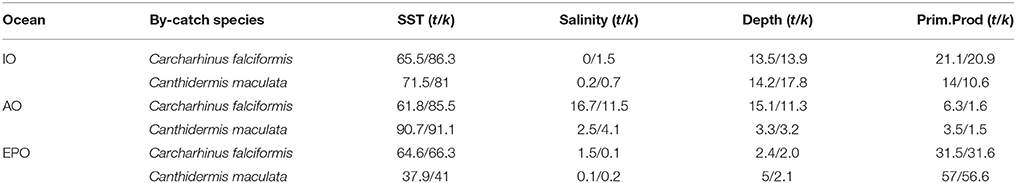
Table 3. Logistitc model output values: percentage of contribution of each environmental variable with all observations (t) and cross-validated (k) for Carcharhinus falciformis and Canthidermis maculata in the Indian (IO), Atlantic (AO), and Eastern Pacific Ocean (EPO).

Sea surface temperature and depth were respectively the most important predictors for silky shark (86.3 and 13.9%) and rough triggerfish (81 and 17.8%) in the habitat models in the Indian Ocean. Sea surface temperature and salinity were the variables that most contributed to the model for silky shark (85.5 and 11.5%) and rough triggerfish (91.1 and 4.1%) in the Eastern Atlantic Ocean. Finally, in the Eastern Pacific Ocean, sea surface temperature was the most important variable for silky shark with 66.3% contribution and primary production for rough triggerfish (56.6%). In general, sea surface temperature was the variable that most contributed to explain the habitat distribution for the two species in each ocean (Table 3).

The relationships between presence probability and environmental variables for each Ocean are illustrated in Figures 3, 4. Silky shark and rough triggerfish presence probability increased with sea surface temperature and decreased linearly with salinity, whereas non-linear relationships were found in some cases for depth and primary production. Concretely, maximum presence probability was found at high temperatures (26–30°) and low salinities (20–30 psu) for both by-catch species in all oceans. Both by-catch species showed preference by deep ocean regions (5000–6000 m) in the Indian Ocean and by intermediate deep regions (3000–4000 m) in the Atlantic and Pacific Ocean (with the exception of silky shark in the Atlantic; its presence probability decreased with depth). Furthermore, probability of presence for both species was found to be higher at low primary production concentrations (50–100 mg·m⁻³) in the Indian Ocean, intermediate concentrations (100–150 mg·m⁻³) in the Atlantic Ocean and at high concentrations (200–300 mg·m⁻³) in the Pacific Ocean.

FIGURE 3

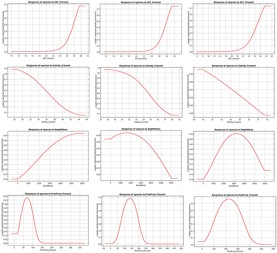
Figure 3. Present response curves (sea surface temperature, salinity, depth, and primary production) for Carcharhinus falciformis in the Indian (first column), Atlantic (second column), and Eastern Pacific Ocean (third column).

FIGURE 4

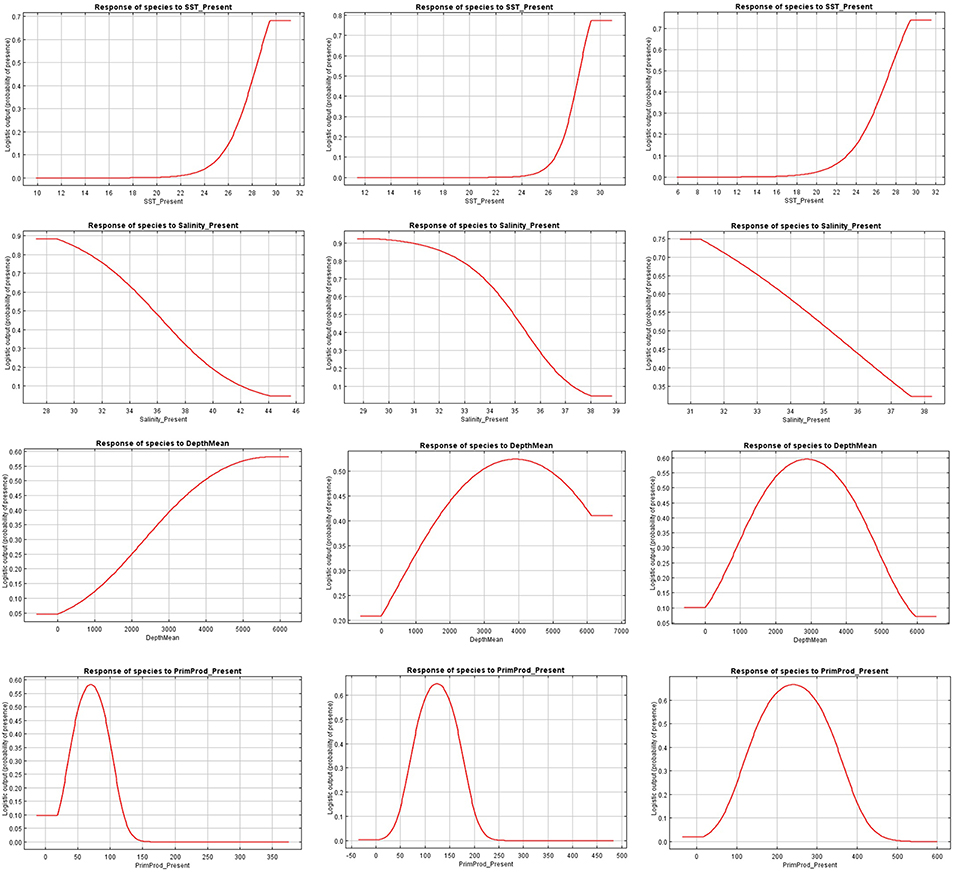
Figure 4. Present response curves (sea surface temperature, salinity, depth, and primary production) for Canthidermis maculata in the Indian (first column), Atlantic (second column), and Eastern Pacific Ocean (third column).

Model Evaluation

AUC values and accuracy indexes for all-observations (t) and cross-validated (k) models are shown in Table 4. MaxEnt models for both species in all oceans showed good agreement between AUC values (0.60–0.80) and accuracy values for cross-validated models (0.50–0.75). The intermediate-high accuracy values for cross-validated models, compared with the models using all observations, indicate that the models were not over-fitted. Sensitivity and specificity values for all observations and cross-validated models showed slightly high values for both species, with the exception of the Indian Ocean (around 0.55), where these values were lower (Table 4). The omission error was low in general (0.05–0.08), indicating that the model performed well. Finally, low-intermediate threshold values were obtained in all cases (around 0.45), showing good proportion of predicted area suitability (Pearson, 2007).

TABLE 4

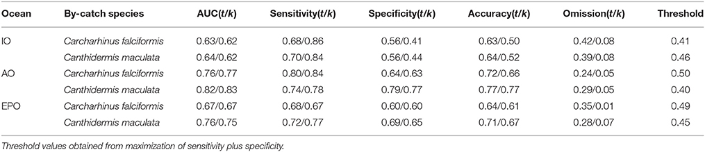
Table 4. Model evaluations with all observations (t) and cross-validated (k) for Carcharhinus falciformis and Canthidermis maculata in the Indian (IO), Atlantic (AO), and Eastern Pacific Ocean (EPO).

In general, distribution models for both by-catch species showed reasonable model performance, although rough triggerfish showed better accuracy values (between 0.60 and 0.80) than silky shark (around 0.60–0.70) in each Ocean. At the same time, the Indian Ocean had the worst performance values (around 0.50–0.60) for both by-catch species in comparison with the Atlantic (0.7/0.8) and Pacific Oceans (0.65/0.75). Finally, to verify that the occurrences randomly taken in the Pacific Ocean were a good representation of the species distribution, the model it was run several times with different sets of 1000 occurrences. In all cases, the results showed high accuracy values.

Projected Habitat Suitability Differences

The projected habitat suitability maps for C. falciformis and C. maculata under A2 future scenario of climate change and differences between future and present conditions (binary maps) for each Ocean are depicted in Figures 1, 2, respectively. The percentages of suitable and loss/gain habitat suitability for silky shark and rough triggerfish in the Indian, Atlantic, and Pacific Oceans are shown in Table 5.

TABLE 5

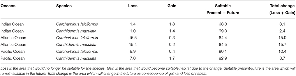
Table 5. Predicted changes in habitat suitability areas (in %) by the year 2100 for the A2 scenario of climate change for both by-catch species.

Under the A2 scenario for 2100, 3.1% of the present habitat for silky shark was predicted to change in the future in the Indian Ocean (Table 5 and Figure 1). The gained areas were mostly located in the south (mostly around 12°S) while the lost areas were located near the Somali coast, the central part of the study area and the south of India. In the Eastern Atlantic Ocean, under climate change impacts, the model predicts that silky shark could gain some habitat north of the equator and in the Cap Lopez area and would loss habitat around the equatorial band between 0 and 10°S (Table 5, Figure 1), with a total change of the present habitat of 15.9%. In the Eastern Pacific Ocean, under the A2 scenario of climate change, 10.4% of the present habitat was predicted to change in the future. Habitat is predicted to be lost near the coastal upwelling area of Peru, and in the equatorial band (10°N and 10°S), while the gains would occur north and south of the Equator (10°N and 10°S) and along the coast of Central America (Nicaragua, Costa Rica, Panamá, Colombia) in an area called “Panama Bight” (Forsbergh, 1969).

On the other hand, because of changes in oceanographic conditions, 2.4% of the present habitat was predicted to change in the future for rough triggerfish in the Indian Ocean. The gained and lost areas were detected in similar areas as for silky sharks. In the Eastern Atlantic Ocean, under the climate change scenario used, 15.7% of the present habitat was predicted to change in the future. The climatic model for 2100 projected a potential gain for rough triggerfish of habitat in the Cap Lopez area and the north of the Equator and loss of habitat in the north (0–10°N/20–40°W) and south (0–10°S/0–10°E) of the Equator. Finally, under the A2 scenario of climate change, 8.7% of the present habitat in the Pacific was predicted to change in the future; with an increase in suitable habitat in the north and south of Equator (around 90–110 and 125–140°W). The model predicted loss of habitat at south of Equator (around 100–110°W) and in the coastal upwelling area of Peru (Table 5, Figure 2).

Discussion

The influence of fishing pressure and climate change on marine ecosystems and more particularly on species distribution has become a general concern (Jones et al., 2013). In this study, we show that species distribution habitats for common and threatened by-catch species can be modeled using MaxEnt species distribution model, even with a limited set of environmental variables. The application of SDM on by-catch species opens a new range of possibilities to study more pelagic species in different areas and fisheries. Potential habitat of species fished in different fisheries could provide important information about species distribution range in the open sea and useful for spatially structured management plans.

We obtained reasonable accurate values using MaxEnt species distribution model, as Peavey (2010) and Sequeira et al. (2012) did. Moderately high AUC and overall prediction accuracy around 0.70 were found for both by-catch species in different oceans. Our distribution models were able to predict habitat suitability for silky shark and rough triggerfish over a more extensive area than that covered only by the observer data (ocurrences). The observer dataset we used contained only silky shark and rough triggerfish presences. We addressed this drawback by randomly generating pseudo-absences (Senay et al., 2013) and running five times the prediction to account for the robustness of the models. However, the correct selection of pseudo-absence data directly affects the accuracy of model prediction. For that reason, the accurate identification of the area (in this case, the sampled area and not areas out of the sampled area) for the creation of pseudo-absences was essential for the correct model performance.

Habitat Suitability Areas

The analysis and modeling of by-catch data collected by observer programs has provided predictions of the pelagic distribution of two wide-ranging species. Thus, the predictive maps produced by our models revealed that the regions close to equatorial and upwelling regions were the most suitable habitats for these species in the Atlantic, Indian, and Pacific Ocean in correspondence to the main fishing grounds. These areas are the most important in the tropical tuna purse seine fisheries (Hall and Roman, 2013) because they are characterized by warm waters, strong surface currents, upwelling systems, and different wind patterns supporting a great variety of organisms and in consequence, high marine biodiversity. Lezama-Ochoa et al. (2015) and Torres-Irineo et al. (2014) showed that higher numbers of species were found close to coastal upwelling areas in the Indian Ocean associated to the monsoon system and with the equatorial counter-current in the Atlantic Ocean. In the Pacific Ocean, the higher numbers of species were found at north of the Equator (10°N) in an area of marked frontal systems and near the coast of Central America (mainly Costa Rica and Panama) [(Lezama-Ochoa et al., 2015, submitted)]. Our results suggest that the distributions of these two species coincide with the areas where the highest biodiversity was found.

It is important to note that the use of this type of data is valid since the information provided by the models reveals interesting findings. Results showed some areas which can be suitable for these species independent of the area of fishing effort. That means these models provide new information (for example, at south (20°S–80°E) and close to the Indian Continent in the Western Indian Ocean, or the coast of Nigeria and Cameroon in the Atlantic Ocean) of areas which can be suitable despite not being fished. In contrast, other areas (for example, north and south (15°N–20°S) in the Atlantic Ocean) which are located inside the fishing effort area are not suitable for these species. It means that both target and non-target species may have different habitat distributions and preferences.

This study was compared with the results from Froese and Pauly (2014) from AquaMaps (Kaschner et al., 2008). Both works showed similar habitat preferences of C. falciformis around coastal and oceanic upwelling waters. However, Froese and Pauly (2014) did not show any climatic projection for the future. In the case of C. maculata, the habitat distribution published by Froese and Pauly (2014) only frames the coastal areas, which results in different distribution ranges and future projections compared with our work. The differences were based on the different sources of information used (museum collections, different databases, literature references) compared to our work which contains a large number of offshore observations since it is based on observer programs covering the wide distribution of the tropical tuna fisheries. In that sense, the presence data of our sampling provides new information about the distribution of the two species. This new information may be a result of the expansion of the FAD fisheries.

The habitat models derived in this study suggest that C. falciformis and C. maculata responded mainly to variation in SST in the three oceans. These by-catch species are often distributed in warm waters and aggregated around floating objects (e.g., logs, Fish Aggregating Devices) in productive areas (Dagorn et al., 2013).

In the Western Indian Ocean, the monsoon system determines the wind and current patterns of the area, with coastal upwelling systems close to Somalia in summer and Mozambique in winter. These systems are associated with changes in the surface temperatures and therefore, affect the habitat and distribution of the by-catch species. In addition, the depth of the ocean basins seems to play an important role in the habitat distribution of both by-catch species. The continental shelf in the Indian Ocean is narrower than in the other oceans and therefore, the distribution of the species in open ocean is close to the coast (Tomczak and Godfrey, 2003).

In the Atlantic Ocean, the SST is also the most important environmental variable followed by low salinity and high primary production concentrations as a consequence of the Benguela upwelling system (Tomczak and Godfrey, 2003).

In the Eastern Pacific Ocean, the SST plays an important role in relation with ENSO conditions in equatorial and coastal upwelling areas of the Pacific. Thus, determines tuna, other teleost species and shark distributions around the “warm pool” area close to the Gulf of Tehuantepec and Central America (Martínez Arroyo et al., 2011). In addition, the primary production is also important in the Eastern Pacific Ocean. The equatorial and Peru eastern boundary currents are associated with highly productive upwelling systems, which form some of the most important fishing areas of the world (Fiedler, 1992). Thus, these environmental variables had important implications on the biogeographic patterns of both species abundance and distribution in each Ocean.

Projected Habitat Suitability

The Intergovernmental Panel on Climate Change (IPCC) estimates ocean warming in the top 100 m between 0.6 and 2.0°C by the end of the twenty-first century (Collins et al., 2013). Species may respond to climate change by shifting their geographical or bathymetric distributions (horizontal or vertical distributions) depending on the extent of the species geographical ranges, dispersal mechanism, life-history strategies, genetic adaptations, and biotic interactions or extinction factors (Thuiller, 2004).

Our results suggest that climate change will affect the distribution of these species depending on the oceanographic conditions of each Ocean. In this study, changes in species distribution as a consequence of climate change were predominant around the equatorial band and in some cases, around upwelling systems [Panama in the Eastern Pacific Ocean, Benguela in the Atlantic Ocean (in a lesser extent)] where fisheries are quite significant. This is not in agreement with the general expectations of migration to deeper waters and poleward shifting of marine fishes in response to sea warming (Walther et al., 2002; Cheung et al., 2013). Moreover, climate change can impact the strength, direction and behavior of the world's main currents and therefore, affecting also in this way the species geographical distributions (Hoegh-Guldberg and Bruno, 2010).

Habitat Loss

The percentage of habitat suitability that could disappear, or persist for each species is a good way to assess the potential impact of climate change at a regional scale (Thuiller, 2004).

If we focus on the habitats in each ocean, the Atlantic Ocean temperatures are projected to increase due to the much larger warming associated with increases of greenhouse gases in this region (Change, 2007); and therefore, a greater and faster loss of habitat in this area is expected. In the case of the Western Indian Ocean, the area around the Somali coastal upwelling system could be unsuitable for the two species as a response to temperature warming, affecting one of the most diverse areas for these by-catch species (Amandè et al., 2011; Lezama-Ochoa et al., 2015).

With regard to the Eastern Pacific Ocean, the A2 climate change scenario projected habitat losses around 8–10% for both by-catch species around the coast of Peru and north and south of the Equator (10°N–10°S). In that sense, some authors suggested a reduction of primary production around these areas as consequence of global warming (Gregg et al., 2003; Hoegh-Guldberg and Bruno, 2010; Blanchard et al., 2012). The results obtained in this work lead us to suggest that these zones could be not suitable for studied by-catch species by 2100 if the primary production is reduced; since these species depend on high nutrient levels and the preys associated to those conditions.

Habitat Gain

Climate change induced some positive effects with gain of habitat for both species in each Ocean. According to Bindoff et al. (2007), the Indian Ocean has been warming in the last years except for an area located at the latitude 12°S along the South Equatorial Current. Therefore, it is believed that this trend will continue in the future. In that sense, our model projects a slight potential colonization for the two by-catch species along this area (12°S) as a consequence of the positive effect of the ocean warming.

C. falciformis and C. maculata could gain new habitat in the Atlantic Ocean near the Angola and Namibia coasts. Global warming could increase the evaporation and, therefore, the rainfall with a consequent increase in the flow of the rivers, providing nutrients to feed plankton in the coastal areas (Justic et al., 1998). Thus, the area located near the mouth of the Congo River could increase its productivity and, hence, the habitat suitability for by-catch species. Other possible explanation for the increase in primary production in the western coast of Africa could be that suggested by Hjort et al. (2012) who showed that an increase in upwelling-favorable winds in the Benguela system could increase primary production. This could benefit the habitat suitability for some species around this area due to an increase of nutrients supplies.

In the Eastern Pacific Ocean, a significant gain of habitat suitability for both by-catch species as a consequence of the increase in primary productivity around Central America is expected by the end of the century. In this region, the temperature increase in the continent as a consequence of global warming will be higher than in the open ocean, which could increase wind intensity favoring upwelling in the coast of Central America where three “wind corridors” play a major role in coastal production (Martínez Arroyo et al., 2011).

In general, there were not significant differences between the percentages of habitat loss and habitat gain for each by-catch species. High percentage of change of habitat was found in the Atlantic Ocean, and a lesser extent, in the Pacific Ocean. In contrast, the Indian Ocean didn't show any relevant change on their distributions. The global warming could impact more the equatorial areas from the Pacific and Atlantic Oceans, which share similar oceanographic features (Tomczak and Godfrey, 2003). The environmental processes in the tropical Indian Ocean, in contrast, seem to play a different role in the diversity (Lezama-Ochoa et al., 2015) and the habitat of the by-catch communities as consequence of the strongest monsoon on Earth. For that reason, the results were expected to be also different. The lack of the permanent equatorial upwelling in the Indian Ocean (as consequence of the steady equatorial easterlies) and the position of the land mass in the north area, seems to influence in the oceanography and environment of this area (Tomczak and Godfrey, 2003).

In an environmental or fisheries management context the question is not necessarily how the climate or ocean abiotic conditions will change, but how the species of the ecosystem might respond to these changes (Payne et al., 2015). We obtained that both by-catch species respond in similar way to the future climate changes. However, with respect to their populations, the silky shark could be largely affected in the Atlantic and the Pacific Ocean if no management measure is taken to reduce its mortality. Silky shark population should be considered more cautiously since this is a vulnerable species less resilient to climate change than small body-size organisms (Lefort et al., 2015). The use of good practices onboard (Gilman, 2011) to increase the post-release survivorship is the best option to reduce their mortality. In addition, understanding its spatio-temporal distribution will help to develop spatially structured mitigation or management measures.”

In contrast, although a similar percentage of habitat loss occurred in triggerfish, their population seems to be stable due to its “r” life-strategy. Even so, it must take into account these species in the future management plans.

Limitation of the Work

Accurately describing and understanding the processes that determine the diversity and distribution of organisms is a fundamental problem in ecology and always inevitably associated with a degree of uncertainty (Payne et al., 2015). This uncertainty is multifaceted and can be decomposed into several elements. Identifying these different factors helps to better address them for obtaining a better model performance. Two of the most important uncertainties in species distribution models (considered as empirical models, see Payne et al., 2015) are structural and scenario uncertainties. Thus, the quality of model outputs can depend on the variables (biological data and environmental data) and the space-time scale considered (Phillips et al., 2009; Payne et al., 2015). There is not best model, and the choice should be driven by the question and the objective of the study.

In this work, the MaxEnt habitat modeling method allowed in an easy way to obtain essential information with few environmental variables about pelagic species. However, the gained experience leads us to discuss several aspects which must be considered and improved applying future habitat models. The selection of the occurrence by-catch data from the fishery not targeting those species can lead to assume that the data quality is not enough. However, we demonstrated that observer data is been used in multiple ecological and habitat studies similar to the one described here. Nevertheless, further increase of the coverage rates (in the case of the Atlantic and Indian Ocean) and the sample size is essential for doing comparisons between years and periods.

The selection of the environmental variables was based in the main oceanographic characteristics of each Ocean, and thus, as showed by the results, the response curves explained correctly the high mobility character of the species and their relationship with the upwelling and surface current systems. However, the selection of other environmental variables related with the ecology of the species (nutrients, oxygen, etc…) could also improve the results. The habitat model performed better at large spatial scales (in the Atlantic and the Pacific Ocean) than at small scales (Indian Ocean). The complex oceanographic processes in the Indian Ocean compared with the Atlantic and Pacific Ocean, which share some oceanographic features, could difficult the selection of specific factors which explain the distribution of the two by-catch species. Thus, a better selection of the environmental data and the application of the other habitat models to compare predictions in this Ocean would be further recommended.

Secondly, the lack of absence data was the most important factor discussed and considered in this study. As we know that the model with presences and absences performs better than the only-presence models, we decided to generated and include the pseudo-absences to evaluate the models. Within the numerous ways of addressing the problem of generate pseudo-absences (Barbet-Massin et al., 2012; Sequeira et al., 2012; Fourcade et al., 2014), here it was solved with the generation of the same number of pseudo-absences (randomly) as presences in places where presences were not observed within the sampled area. However, in future works, it would be worth to compare among different ways to generate pseudo-absences.

The Applicability of Habitat Models on Fisheries Management Plans

By-catch is a significant issue for the fishing industry, scientists and managers, and it needs to be managed and mitigated. Invasions and extinctions of by-catch species in an area can affect not only their species distribution range, but also the marine biodiversity, community structure, size spectra, and ecosystem functions (Sala and Knowlton, 2006). In this context, by-catch monitoring programs with observers onboard can be expensive and sometimes difficult to implement. However, they are an important source of data to identify suitable habitats to be used in conservation biology field (Franklin and Miller, 2009).

Thus, there is still a need to develop SDM for other by-catch species and/or habitats of interest for these species (e.g., upwelling areas, seamounts, coastal areas) to investigate their spatial distributions and to assess the effects that fishing and climate change may have on those populations. Concretely, it would be interesting to apply this habitat model in other tuna target-species to describe their potential habitat distribution and identify any possible overlap with the by-catch species. Thus, the future gain areas by the by-catch species, provided that target species distribution remains the same, could be act as a refuge for by-catch species. Similarly, those losses areas could be considered to be protected in future management plans. Moreover, other habitat suitability distribution approaches (such as ensembles of different algorithms) and other more sophisticated and descriptive environmental predictors, as well as new climate change scenarios may help to improve habitat distribution projections.

Monitoring and understanding changes in by-catch species distributions, in addition to those of the harvested species (tunas), are necessary for a better understanding of the pelagic ecosystem and toward a correct implementation of the EAFM.

Conclusions

Our model predicts that potential habitat distribution areas for C. falciformis and C. maculata in the Atlantic, Indian, and Pacific Oceans are close to equatorial and coastal upwelling areas, and mainly associated with sea surface temperature. These habitat distribution models, based on the information collected by observer programs from the tropical tuna purse seine fisheries in the three oceans, provide a good estimation of the pelagic distribution of these wide-ranging by-catch species. The global ocean warming could impact some of these unstable and vulnerable ecosystems (mainly in the Atlantic and the Pacific Ocean) affecting the distribution of these species in accordance with the particular oceanographic conditions of each Ocean. Under climate change scenarios, the largest change in present habitat suitability was observed in the Atlantic Ocean (around 16% of the present habitat suitability area of C. falciformis and C. maculata) whereas the change was less in the Pacific Ocean (around 10 and 8%) and any significant change was observed in the Indian Ocean (around 3 and 2%).

Author Contributions

NL, HM, GC, EVL, MH and EV designed research; NL, HM, GC and EV performed research; NL analyzed data; and NL, HM, GC, EVL, JR, MH, PC, AD and EV wrote the paper.

Conflict of Interest Statement

The authors declare that the research was conducted in the absence of any commercial or financial relationships that could be construed as a potential conflict of interest.

Acknowledgments

The occurrence data analyzed in this study were collected by AZTI, Institut de Recherche pour le Développement (IRD), Instituto Español de Oceanografía (IEO), and IATTC (Inter American Tropical Tuna Commission) through the EU- funded Data Collection Framework (DCF, Reg (EC) 1543/2000, 1639/2001, and 665/2008) and IATTC observer program. We wish to acknowledge to Nick Vogel (IATTC) for the process and management of the by-catch data and especially to Maite Louzao for her help and advices with the analyses. This study was part of the Ph.D. thesis conducted by the first author (NLO) at AZTI marine institute and funded by Iñaki Goenaga (FCT grant). The authors declare that the research was conducted in the absence of any commercial or financial relationships that could be construed as a potential conflict of interest. This is contribution 759 from AZTI Marine Research Division.

Supplementary Material

The Supplementary Material for this article can be found online at: https://www.frontiersin.org/article/10.3389/fmars.2016.00034

References

Amandè, J. M., Ariz, J., Chassot, E., Chavance, P., Delgado De Molina, A., Gaertner, D., et al. (2008). “By-catch and discards of the European Purse Seine Tuna Fishery in the Indian Ocean: estimation and characteristics for the 2003–2007 period,” in IOTC Proceedings IOTC-2008-WPEB-12 (Bangkok).

Amandè, M. J., Ariz, J., Chassot, E., De Molina, A. D., Gaertner, D., Murua, H., et al. (2010). Bycatch of the European purse seine tuna fishery in the Atlantic Ocean for the 2003–2007 period. Aquat. Living Resour. 23, 353–362. doi: 10.1051/alr/2011003

CrossRef Full Text | Google Scholar

Amandè, M. J., Bez, N., Konan, N., Murua, H., Delgado De Molina, A., Chavance, P., et al. (2011). “Areas with high bycatch of silky sharks (Carcharhinus falciformis) in the Western Indian Ocean purse seine fishery,” in IOTC Proceedings IOTC–2011–WPEB (Lankanfinolhu), 7.

Google Scholar

Amandè, M., Chassot, E., Chavance, P., and Planet, R. (2008). “Silky shark (Carcharhinus falciformis) bycatch in the French tuna purse-seine fishery of the Indian Ocean,” in IOTC Proceedings IOTC-2008-WPEB-16 (Bangkok), 22.

Anderson, R. P., Dudík, M., Ferrier, S., Guisan, A. J., Hijmans, R., Lohmann, L., et al. (2006). Novel methods improve prediction of species' distributions from occurrence data. Ecography 29, 129–151. doi: 10.1111/j.2006.0906-7590.04596.x

CrossRef Full Text | Google Scholar

Arrizabalaga, H., Dufour, F., Kell, L., Merino, G., Ibaibarriaga, L., Chust, G., et al. (2015). Global habitat preferences of commercially valuable tuna. Deep Sea Res. Part II Top. Stud. Oceanogr. 113, 102–112. doi: 10.1016/j.dsr2.2014.07.001

CrossRef Full Text | Google Scholar

Barbet-Massin, M., Jiguet, F., Albert, C. H., and Thuiller, W. (2012). Selecting pseudo-absences for species distribution models: how, where and how many? Methods Ecol. Evol. 3, 327–338. doi: 10.1111/j.2041-210X.2011.00172.x

CrossRef Full Text

Bindoff, N. L., Willebrand, J., Artale, V., Cazenave, A., Gregory, J. M., Gulev, S., et al. (2007). Observations: Oceanic Climate Change and Sea Level. Cambridge, UK: Cambridge University Press.

Google Scholar

Blanchard, J. L., Jennings, S., Holmes, R., Harle, J., Merino, G., Allen, J. I., et al. (2012). Potential consequences of climate change for primary production and fish production in large marine ecosystems. Philos. Trans. R. Soc. B Biol. Sci. 367, 2979–2989. doi: 10.1098/rstb.2012.0231

PubMed Abstract | CrossRef Full Text | Google Scholar

Castro, J. J., Santiago, J. A., and Santana-Ortega, A. T. (2002). A general theory on fish aggregation to floating objects: an alternative to the meeting point hypothesis. Rev. Fish Biol. Fish 11, 255–277. doi: 10.1023/A:1020302414472

CrossRef Full Text | Google Scholar

Change, I. P. O. C. (2007). Climate Change 2007: The Physical Science Basis. Agenda. Vol. 6. Cambridge, UK: Cambridge University Press.

Cheung, W. W., Pinnegar, J., Merino, G., Jones, M. C., and Barange, M. (2012). Review of climate change impacts on marine fisheries in the UK and Ireland. Aquat. Conserv. Mar. Freshw. Ecosyst. 22, 368–388. doi: 10.1002/aqc.2248

CrossRef Full Text | Google Scholar

Cheung, W. W., Watson, R., and Pauly, D. (2013). Signature of ocean warming in global fisheries catch. Nature 497, 365–368. doi: 10.1038/nature12156

PubMed Abstract | CrossRef Full Text | Google Scholar

Chust, G., Castellani, C., Licandro, P., Ibaibarriaga, L., Sagarminaga, Y., and Irigoien, X. (2014). Are Calanus spp. shifting poleward in the North Atlantic? A habitat modelling approach. ICES J. Mar. Sci. 71, 241–253. doi: 10.1093/icesjms/fst147

CrossRef Full Text | Google Scholar

Collins, M., Knutti, R., Arblaster, J., Dufresne, J.-L., Fichefet, T., Friedlingstein, P., et al. (2013). Long-Term Climate Change: Projections, Commitments and Irreversibility. Cambridge, UK; New York, NY: Cambridge University Press.

Google Scholar

Commission, I. S. S. (2000). IUCN Red List of Threatened Species. Gland: The World Conservation Union.

Google Scholar

Dagorn, L., Holland, K. N., Restrepo, V., and Moreno, G. (2013). Is it good or bad to fish with FADs? What are the real impacts of the use of drifting FADs on pelagic marine ecosystems? Fish Fish. 14, 391–415. doi: 10.1111/j.1467-2979.2012.00478.x

PubMed Abstract | CrossRef Full Text | Google Scholar

Dayton, P. K., Thrush, S. F., Agardy, M. T., and Hofman, R. J. (1995). Environmental effects of marine fishing. Aquat. Conserv. Mar. Freshw. Ecosyst. 5, 205–232. doi: 10.1002/aqc.3270050305

CrossRef Full Text | Google Scholar

Duffy, L. M., Olson, R. J., Lennert-Cody, C. E., Galván-Magaña, F., Bocanegra-Castillo, N., and Kuhnert, P. M. (2015). Foraging ecology of silky sharks, Carcharhinus falciformis, captured by the tuna purse-seine fishery in the eastern Pacific Ocean. Mar. Biol. 162, 571–593. doi: 10.1007/s00227-014-2606-4

CrossRef Full Text | Google Scholar

Elith, J., and Leathwick, J. R. (2009). Species Distribution models: ecological explanation and prediction across space and time. Annu. Rev. Ecol. Evol. Syst. 40, 677–697. doi: 10.1146/annurev.ecolsys.110308.120159

CrossRef Full Text | Google Scholar

Elith, J., Phillips, S. J., Hastie, T., Dudík, M., Chee, Y. E., and Yates, C. J. (2011). A statistical explanation of MaxEnt for ecologists. Divers. Distrib. 17, 43–57. doi: 10.1111/j.1472-4642.2010.00725.x

CrossRef Full Text | Google Scholar

Fiedler, P. C. (1992). Seasonal Climatologies and Variability of Eastern Tropical Pacific Surface Waters. NOAA Technical Report NMFS, 109. NOAA/National Marine Fisheries Service.

Fiedler, P. C. (2002). Environmental change in the eastern tropical Pacific Ocean: review of ENSO and decadal variability. Mar. Ecol. Prog. Ser. 244, 265–283. doi: 10.3354/meps244265

CrossRef Full Text | Google Scholar

Fielding, A. H., and Bell, J. F. (1997). A review of methods for the assessment of prediction errors in conservation presence/absence models. Environ. Conserv. 24, 38–49. doi: 10.1017/S0376892997000088

CrossRef Full Text | Google Scholar

Forsbergh, E. (1969). Estudio sobre la climatología, oceanografía y pesquerías del Panamá Bight. Comisión Interamericana del Atún Tropical 14, 49–364.

Fourcade, Y., Engler, J. O., Rödder, D., and Secondi, J. (2014). Mapping species distributions with MAXENT using a Geographically biased sample of presence data: a performance assessment of methods for correcting sampling bias. PLoS ONE 9:e97122. doi: 10.1371/journal.pone.0097122

PubMed Abstract | CrossRef Full Text | Google Scholar

Franklin, J., and Miller, J. A. (2009). Mapping Species Distributions. Spatial Inference and Prediction. Cambridge: Cambridge University Press.

Google Scholar

Fréon, P., and Dagorn, L. (2000). Review of fish associative behaviour: toward a generalisation of the meeting point hypothesis. Rev. Fish Biol. Fish 10, 183–207. doi: 10.1023/A:1016666108540

CrossRef Full Text | Google Scholar

Froese, R., and Pauly, D. (2014). FishBase. 2014. World Wide Web Electronic Publication. Available online at: www.fishbase.org, version 6.

Gaertner, D., Ménard, F., Develter, C., Ariz, J., and Delgado De Molina, A. (2002). Bycatch of billfishes by the European tuna purse seine-fishery in the Atlantic Ocean. Fish. Bull. 100, 683–689. doi: 10.1051/alr/2011003

CrossRef Full Text | Google Scholar

Gerrodette, T., Olson, R., Reilly, S., Watters, G., and Perrin, W. (2012). Ecological metrics of biomass removed by three methods of Purse-Seine fishing for Tunas in the Eastern Tropical Pacific ocean. Conserv. Biol. 26, 248–256. doi: 10.1111/j.1523-1739.2011.01817.x

PubMed Abstract | CrossRef Full Text | Google Scholar

Gilman, E. L. (2011). Bycatch governance and best practice mitigation technology in global tuna fisheries. Mar. Policy 35, 590–609. doi: 10.1016/j.marpol.2011.01.021

CrossRef Full Text | Google Scholar

Girard, C., Benhamou, S., and Dagorn, L. (2004). FAD: fish aggregating device or fish attracting device? A new analysis of yellowfin tuna movements around floating objects. Anim. Behav. 67, 319–326. doi: 10.1016/j.anbehav.2003.07.007

CrossRef Full Text | Google Scholar

Gregg, W. W., Conkright, M. E., Ginoux, P., O'reilly, J. E., and Casey, N. W. (2003). Ocean primary production and climate: global decadal changes. Geophys. Res. Lett. 30:1809. doi: 10.1029/2003GL016889

CrossRef Full Text | Google Scholar

Hall, M., and Roman, M. (2013). Bycatch and Non-Tuna Catch in the Tropical Tuna Purse Seine Fisheries of the World. FAO Fisheries and Aquaculture Technical Paper, 568.

Hijmans, R. J., Phillips, S., Leathwick, J., Elith, J., and Hijmans, M. R. J. (2013). Package ‘dismo’, Circles Vol. 9. R. sofware.

Hijmans, R. J., and Van Etten, J. (2012). raster: Geographic Analysis and Modeling with Raster Data. R package version, Vol. 1, 9–92.

Hjort, A., Sheridan, S., and Davies, S. (2012). Climate Change Implications for Fisheries of the Benguela Current Region: Making the Best of Change? Rome: Food and Agriculture Organization of the United Nations.

Hoegh-Guldberg, O., and Bruno, J. F. (2010). The impact of climate change on the world's marine ecosystems. Science 328, 1523–1528. doi: 10.1126/science.1189930

PubMed Abstract | CrossRef Full Text | Google Scholar

Jiménez-Valverde, A., and Lobo, J. M. (2007). Threshold criteria for conversion of probability of species presence to either–or presence–absence. Acta Oecol. 31, 361–369. doi: 10.1016/j.actao.2007.02.001

CrossRef Full Text | Google Scholar

Jones, M. C., Dye, S. R., Fernandes, J. A., Frölicher, T. L., Pinnegar, J. K., Warren, R., et al. (2013). Predicting the impact of climate change on threatened species in UK waters. PLoS ONE 8:e54216. doi: 10.1371/journal.pone.0054216

PubMed Abstract | CrossRef Full Text | Google Scholar

Justic, D., Rabalais, N., and Turner, R. (1998). Impacts of climate change on net productivity of coastal waters: implications for carbon budgets and hypoxia. Clim. Res. 8, 225–237.

Google Scholar

Kaschner, K., Ready, J., Agbayani, E., Rius, J., Kesner-Reyes, K., Eastwood, P., et al. (2008). AquaMaps: Predicted Range Maps for Aquatic Species. World Wide Web Electronic Publication. Available online at: www.aquamaps.org, Version 8, 2010.

Kelleher, K. (2005). Discards in the World's Marine Fisheries: An Update. Rome: Food & Agriculture Org.

Google Scholar

Khanum, R., Mumtaz, A., and Kumar, S. (2013). Predicting impacts of climate change on medicinal asclepiads of Pakistan using Maxent modeling. Acta Oecol. 49, 23–31. doi: 10.1016/j.actao.2013.02.007

CrossRef Full Text | Google Scholar

Kohavi, R. (1995). A Study of Cross-Validation and Bootstrap for Accuracy Estimation and Model Selection. Montreal, QC: IJCAI.

Google Scholar

Komoroske, L., and Lewison, R. (2015). Addressing fisheries bycatch in a changing world. Front. Mar. Sci 2:83. doi: 10.3389/fmars.2015.00083

CrossRef Full Text | Google Scholar

Kumar, S., and Stohlgren, T. J. (2009). Maxent modeling for predicting suitable habitat for threatened and endangered tree Canacomyrica monticola in New Caledonia. J. Ecol. Nat. Environ. 1, 94–98. doi: 10.5897/JENE

CrossRef Full Text | Google Scholar

Lefort, S., Aumont, O., Bopp, L., Arsouze, T., Gehlen, M., and Maury, O. (2015). Spatial and body-size dependent response of marine pelagic communities to projected global climate change. Glob. Change Biol. 21, 154–164. doi: 10.1111/gcb.12679

PubMed Abstract | CrossRef Full Text | Google Scholar

Lenoir, S., Beaugrand, G., and Lecuyer, A. (2011). Modelled spatial distribution of marine fish and projected modifications in the North Atlantic Ocean. Glob. Change Biol. 17, 115–129. doi: 10.1111/j.1365-2486.2010.02229.x

CrossRef Full Text | Google Scholar

Lezama-Ochoa, N., Murua, H., Chust, G., Ruiz, J., Chavance, P., De Molina, A. D., et al. (2015). Biodiversity in the by-catch communities of the pelagic ecosystem in the Western Indian Ocean. Biodivers. Conserv. 24, 2647–2671. doi: 10.1007/s10531-015-0951-3

CrossRef Full Text | Google Scholar

Longhurst, A. R., and Pauly, D. (1987). Ecology of Tropical Oceans. San Diego, CA: Academic Press.

Google Scholar

López, J. (2015). Behaviour of Tuna and Non-Tuna Species at Fish Aggregating Devices (FADs), Ascertained through Fishers' Echo-Sounder Buoys: Implications for Conservation and Management. Ph.D. thesis. Department of Zoology and Animal Cell Biology, University of the Basque Country.

Louzao, M., Delord, K., García, D., Boué, A., and Weimerskirch, H. (2012). Protecting persistent dynamic oceanographic features: transboundary conservation efforts are needed for the critically endangered balearic shearwater. PLoS ONE 7:e35728. doi: 10.1371/journal.pone.0035728

PubMed Abstract | CrossRef Full Text | Google Scholar

Martínez Arroyo, A., Manzanilla Naim, S., and Zavala Hidalgo, J. (2011). Vulnerability to climate change of marine and coastal fisheries in México. Atmósfera 24, 103–123.

Google Scholar

Martínez Rincón, R. O. (2012). Efecto de la Variabilidad Ambiental en la Distribución de las Capturas Incidentales de pelágicos Mayores en el Océano Pacífico Oriental. Instituto Politécnico Nacional. Centro Interdisciplinario de Ciencias Marinas.

Martínez-Rincón, R. O., Ortega-García, S., and Vaca-Rodriguez, J. G. (2009). Incidental catch of dolphinfish (C < i> oryphaena </i> spp.) reported by the Mexican tuna purse seiners in the eastern Pacific Ocean. Fish. Res. 96, 296–302. doi: 10.1016/j.fishres.2008.12.008

CrossRef Full Text | Google Scholar

Minami, M., Lennert-Cody, C. E., Gao, W., and Roman-Verdesoto, M. (2007). Modeling shark bycatch: the zero-inflated negative binomial regression model with smoothing. Fish. Res. 84, 210–221. doi: 10.1016/j.fishres.2006.10.019

CrossRef Full Text | Google Scholar

Muthoni, F. K. (2010). Modelling the Spatial Distribution of Snake Species under Changing Climate Scenario in Spain. Enschede: University of Twente.

Google Scholar

Nguyen, T. V. (2012). Ecosystem-Based fishery management: a review of concepts and ecological economic models. J. Ecosyst. Manag. 13, 1–14.

Google Scholar

Payne, M. R., Barange, M., Cheung, W. W., Mackenzie, B. R., Batchelder, H. P., Cormon, X., et al. (2015). Uncertainties in projecting climate-change impacts in marine ecosystems. ICES J. Mar. Sci. doi: 10.1093/icesjms/fsv231

PubMed Abstract | CrossRef Full Text | Google Scholar

Pearson, R. G. (2007). Species' Distribution Modeling for Conservation. American Museum of Natural History.

Google Scholar

Peavey, L. (2010). Predicting Pelagic Habitat with Presence-only Data using Maximum Entropy for Olive Ridley Sea Turtles in the Eastern Tropical Pacific. Masters Thesis, Duke University, North Caroline.

Phillips, S. J., Anderson, R. P., and Schapire, R. E. (2006). Maximum entropy modeling of species geographic distributions. Ecol. Modell. 190, 231–259. doi: 10.1016/j.ecolmodel.2005.03.026

CrossRef Full Text | Google Scholar

Phillips, S. J., Dudík, M., Elith, J., Graham, C. H., Lehmann, A., Leathwick, J., et al. (2009). Sample selection bias and presence-only distribution models: implications for background and pseudo-absence data. Ecol. Appl. 19, 181–197. doi: 10.1890/07-2153.1

PubMed Abstract | CrossRef Full Text | Google Scholar

Poisson, F. (2007). “Compilation of information on blue shark (Prionace glauca), silky shark (Carcharhinus falciformis), oceanic whitetip shark (Carcharhinus longimanus), scalloped hammerhead (Sphyrna lewini) and shortfin mako (Isurus oxyrinchus) in the Indian Ocean,” in 3rd Session of the IOTC Working Party on Ecosystems and Bycatch (Victoria).

Rombouts, I., Beaugrand, G., and Dauvin, J.-C. (2012). Potential changes in benthic macrofaunal distributions from the English Channel simulated under climate change scenarios. Estuar. Coast. Shelf Sci. 99, 153–161. doi: 10.1016/j.ecss.2011.12.026

CrossRef Full Text | Google Scholar

Sala, E., and Knowlton, N. (2006). Global marine biodiversity trends. Annu. Rev. Environ. Resour. 31, 93–122. doi: 10.1146/annurev.energy.31.020105.100235

CrossRef Full Text | Google Scholar

Senay, S. D., Worner, S. P., and Ikeda, T. (2013). Novel three-step pseudo-absence selection technique for improved species distribution modelling. PLoS ONE 8:e71218. doi: 10.1371/journal.pone.0071218

PubMed Abstract | CrossRef Full Text | Google Scholar

Sequeira, A., Mellin, C., Rowat, D., Meekan, M. G., and Bradshaw, C. J. (2012). Ocean-scale prediction of whale shark distribution. Divers. Distrib. 18, 504–518. doi: 10.1111/j.1472-4642.2011.00853.x

CrossRef Full Text | Google Scholar

Sund, P. N., Blackburn, M., and Williams, F. (1981). Tunas and their environment in the Pacific Ocean: a review. Oceanogr. Mar. Biol. Ann. Rev 19, 443–512.

Google Scholar

Thuiller, W. (2004). Patterns and uncertainties of species' range shifts under climate change. Glob. Change Biol. 10, 2020–2027. doi: 10.1111/j.1365-2486.2004.00859.x

CrossRef Full Text | Google Scholar

Thuiller, W., Lavorel, S., and Araújo, M. B. (2005). Niche properties and geographical extent as predictors of species sensitivity to climate change. Glob.l Ecol. Biogeogr. 14, 347–357. doi: 10.1111/j.1466-822X.2005.00162.x

CrossRef Full Text | Google Scholar

Tomczak, M., and Godfrey, J. S. (2003). Regional Oceanography: An Introduction. Oxford, UK: Elsevier.

Google Scholar

Torres-Irineo, E., Amandè, M. J., Gaertner, D., De Molina, A. D., Murua, H., Chavance, P., et al. (2014). Bycatch species composition over time by tuna purse-seine fishery in the eastern tropical Atlantic Ocean. Biodivers. Conserv. 23, 1157–1173. doi: 10.1007/s10531-014-0655-0

CrossRef Full Text | Google Scholar

Villarino, E., Chust, G., Licandro, P., Butenschön, M., Ibaibarriaga, L., Kreus, M., et al. (2015). Modelling the future biogeography of North Atlantic zooplankton communities in response to climate change. Mar. Ecol. Prog. Ser. 531, 121–142.

Google Scholar

Walther, G.-R., Post, E., Convey, P., Menzel, A., Parmesan, C., Beebee, T. J., et al. (2002). Ecological responses to recent climate change. Nature 416, 389–395. doi: 10.1038/416389a

PubMed Abstract | CrossRef Full Text | Google Scholar

Watson, J. T. (2007). Trade-offs in the Design of Fishery Closures: Silky Shark by Catch Management in the Eastern Pacific Ocean Tuna Purse Seine Fishery. University of Washington.

Worm, B., Barbier, E. B., Beaumont, N., Duffy, J. E., Folke, C., Halpern, B. S., et al. (2006). Impacts of biodiversity loss on ocean ecosystem services. Science 314, 787–790. doi: 10.1126/science.1132294

PubMed Abstract | CrossRef Full Text | Google Scholar