Spatial Modeling of Calanus finmarchicus and Calanus helgolandicus: Parameter Differences Explain Differences in Biogeography

1. Introduction

Zooplankton communities are now reorganizing throughout the North Atlantic (Beaugrand et al., 2009; Chust et al., 2013). Rising temperatures are causing species to expand at the northern edge of their distribution, while they are retreating at the southern edge (Beaugrand, 2012). As a consequence, communities are changing and many species are being replaced by their southern congenerics (Beaugrand et al., 2002).

Changes in communities dominated by the calanoid copepods Calanus finmarchicus and C. helgolandicus are among the most well-studied (Wilson et al., 2015). C. finmarchicus is an oceanic species that is found from the Gulf of Maine to the North Sea (Melle et al., 2014). In contrast, C. helgolandicus is a shelf species that lives from the North Sea to the Mediterranean Sea (Bonnet et al., 2005). Both species are now moving north, which has caused C. helgolandicus to replace C. finmarchicus as the dominant calanoid copepod in the North Sea (Reid et al., 2003). Future temperature rises will likely cause this to be repeated further north (Villarino et al., 2015). We must therefore understand differences in the impacts of climate change on congeneric zooplankton species, so that we can anticipate changes in communities and their consequences.

A key test of our understanding of the interspecific differences in demography of these species is whether we can simulate their population dynamics in such a way that the relative geographic distributions of both species are a result of the differences in biology. An inability to do this can highlight important knowledge gaps that must be filled to make projections of the impact of climate change on Calanus communities more biologically credible.

In this spirit, we tested the ability of known interspecific differences to explain the geographic distributions of both species by creating a new unified model. We created a stage-structured model which represents each life stage of C. finmarchicus and C. helgolandicus, and that represents body size by dividing each stage into a set of size classes. This work is based on the previous model of C. finmarchicus in the North Atlantic of Speirs et al. (2005, 2006). Continuous Plankton Recorder survey data was used to parameterize the model and simulated annual cycles of abundance and fecundity were compared with empirical time series in a number of North Atlantic locations.

Recently, an increasing number of researchers have taken a trait-based approach to understanding zooplankton communities (Barton et al., 2013; Litchman et al., 2013). Key traits such as body size, development rate and fecundity are identified, and the functional role of species in ecosystems is thus thought to be a function of their positions within trait-space. A trait-based approach has previously been used to model copepod communities in Cape Cod Bay, Massachusetts (Record et al., 2010). We used this approach to understand the biogeography of two species, under the assumption that where species lie in trait-space is the fundamental determinant of relative biogeography.

Our underlying philosophy is that the equations describing the population dynamics of both species should be identical, but with potential differences in parameters. This constraint will arguably result in suboptimal models for each species when viewed separately. However, it enables us to more clearly understand the biological differences that drive the large-scale differences in distribution. Fundamentally, this work is based on the assumption that if knowledge of key interspecific differences is sufficient, then known interspecific differences are all that is needed for a model to reproduce the geographic distributions of both species. The only known difference between the species that could influence population dynamics is the response of ingestion rate, and thus growth, development and fecundity, to temperature (Wilson et al., 2015). We therefore begin with the hypothesis that this difference alone can explain most of the differences in geographic distribution.

2. Model

2.1. Model Background and Framework

We present an extension of the previous work by Speirs et al. (2005, 2006), who modeled the population dynamics of C. finmarchicus over the entire North Atlantic. This extension took two key forms. First, we incorporated recent developments in our understanding of Calanus biology. Second, we modified the model of Speirs et al. (2006) so that it could represent the population dynamics of both C. finmarchicus and C. helgolandicus. Full mathematical details of the model, along with relevant parameters, are given in Appendix 1 (Supplementary Material). Here we will summarize the modeling framework of Speirs et al. and then the extensions to it.

The model of Speirs et al. was discrete in time and space. It covered the entire North Atlantic, ranging from 30 to 80°N and 80°W to 90°E. The population of C. finmarchicus was distributed over a regular grid of cells of size 0.5°longitude by 0.25°latitude. They had two update processes. First, the population of each cell was updated to account for development, reproduction and mortality. After these updates, the population is redistributed between cells to account for physical population transport. A separate physical model was used to create the flow-field and temperature drivers for the relevant biological and physical update. The annual cycle of food in each cell was estimated by deriving phytoplankton carbon fields from satellite sea-color observations. 1997 was used as the target year for simulations because this was the year when the Trans-Atlantic Study of Calanus (TASC) collected a large number of time series of C. finmarchicus abundance in the North Atlantic. The framework of Speirs et al. was as follows. Surface developers are made up of eggs (E), naupliar stages (N1 to N6), and copepodite stages (C1 to C5). Finally, there are diapausers (C5d) and adults (C6).

Calanus development follows the equiproportional rule, that is relative stage duration is independent of temperature (Campbell et al., 2001). Development from egg to adult can therefore be divided into a fixed number of steps, with each having identical time duration under identical environmental conditions (Gurney et al., 2001). In total, there were 57 development steps, which cover the 13 stages of Calanus development.

This framework allows the entire population to be updated simultaneously, and for the entire population to be simulated with high computational efficiency (Speirs et al., 2006). However, modeling the populations of C. finmarchicus and C. helgolandicus required one modification.

We began with the hypothesis that differences in the response of growth and development to temperature are sufficient to explain the geographic distributions of both species. In other words, all equations and parameters would be the same, except for those related to growth and development. This could not be satisfactorily achieved in the original framework. Large-scale patterns of fecundity are not only the result of the effects of environmental conditions, but also of body size. Further, the ability of animals to diapause is strongly influenced by size (Wilson et al., 2016). We therefore incorporated body size into the framework. Large-scale patterns of fecundity and diapause duration could therefore be represented as the combined effects of body size and the environment, and did not require the introduction of interspecific differences. The geographic domain used by Speirs et al. covers all regions of high C. helgolandicus abundance (Bonnet et al., 2005), and was therefore maintained.

2.2. Biological Processes: A New View of Calanus Biology

The following biological processes are represented in our model: development, egg production, diapause and mortality. In each case, we modified the model of Speirs et al. to account for recent developments in the understanding of Calanus biology.

A recent review of the differences between the two species found that the only known relevant difference was the influence of temperature on ingestion, and thus growth, development and fecundity (Wilson et al., 2015). We therefore constrained the model by making a number of assumptions about the differences between the species based on this review. These assumptions were as follows:

• There is a dome-shaped response of ingestion rate to temperature for both species, with ingestion rate higher for C. finmarchicus than C. helgolandicus below a temperature of 13°C.

• An emergent property of this is that there are dome-shaped relationships between growth and egg production rate and temperature, and a U-shaped relationship between development time and temperature for both species.

• Under identical conditions, both species will grow to the same size.

• There are no differences in the ability to accumulate lipids or diapause.

Further, we take the following assumptions and simplifications about the biology and ecology of both species.

• There are no interactions between the two species.

• The species do not hybridize. However, hybridization has been observed among other Calanus species (Parent et al., 2011, 2012; Gabrielsen et al., 2012).

• The relationships between traits and the environment do not vary in time or space.

The key modeled relationships between body size, development time, egg production rate and diapause duration with temperature are shown in Figure 1.

FIGURE 1

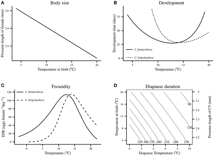
Figure 1. Influence of temperature on Calanus's body size, development and growth in the model. Body size and diapause duration are assumed to be the same in both species. Development time is based on the model of Wilson et al. (2015), and the EPR model is derived from that model's growth equation assuming that female's use carbon for egg production instead of growth. Egg-adult development times assume an animal is of size 280 μg C. (A) Modeled relationship between female body size and temperature at birth for both species. (B) Modeled relationship between egg-adult development time under food-saturated conditions for both species. (C) Modeled relationship between fecundity and temperature for both species. Fecundity relationships assume an animal is of size 280 μg C. (D) Modeled relationship between diapause temperature and prosome length of C5 and diapause temperature for both species. Body size is assumed to be determined by temperature at birth.

There are no apparent interspecific differences in body size, and large-scale geographic patterns of body size are largely driven by temperature (Wilson et al., 2015). We therefore modeled body size under the simplified assumption that it is determined by temperature experienced at birth for all development classes (Figure 1A). This assumption is derived from the fact that egg size is determined by temperature (Campbell et al., 2001) and that the existence of an exo-skeleton likely greatly constrains size over all development classes. The temperature-prosome length relationship of Campbell et al. (2001) was used with a multiplier, which was fitted based on the relationship between predicted and observed female prosome length. Prosome length reduces linearly with increasing temperature. This approach contrasts with Speirs et al., which did not represent size.

Egg-adult development time was assumed to be influenced purely by temperature and food concentration. The relationship between egg-adult development time and temperature under food-saturated conditions is assumed to follow that derived by the model of Wilson et al. (2015). Development time saturates at high food levels, and we use the relationship between food concentration and development time of Campbell et al. (2001). There is a U-shaped response of development time to temperature (Figure 1B), which contrasts with the monotonically decreasing form used by Speirs et al. The computational approach is that of Gurney et al. (2001) and uses dynamic time-step constraints. This is the same approach as in Speirs et al. (2005, 2006) and it is effective in minimizing numerical diffusion (Gurney et al., 2001; Record and Pershing, 2008).

Fecundity was related to temperature, food concentration and body size. We assumed that egg production and growth are equivalent (McLaren and Leonard, 1995). Egg laying females have stopped growing and we therefore assume that carbon previously directed to growth will be used to make eggs. The growth rate equation of Wilson et al. (2015) forms the basis of our egg production rate (EPR) model for both species, with the food saturation component taken from Hirche et al. (1997). EPR therefore has a dome-shaped response to temperature (Figure 1C). Further, EPR has a saturating response to food concentration and we use a conventional allometric relationship between EPR and carbon weight, i.e., EPR ~ carbon weight^0.75. This contrasts with Speirs et al., who represented EPR as a monotonically increasing function of temperature, but using the same food response as we have assumed. We assume that 50% of adults are female.

A recent modeling study, which synthesized empirical findings, showed that maximum potential diapause duration is largely determined by prosome length and overwintering temperature (Wilson et al., 2016). We therefore modeled diapause duration using the maximum potential diapause duration equation from that study (Figure 1D). Diapause duration declines at higher temperature because of increased metabolic rates, and is shorter at smaller prosome lengths because of lower relative lipid levels and higher relative metabolic costs. We assumed that a fraction of the C5 population enters diapause at the end of the C5 stage. This fraction is dependent on growth rate, with it increasing at lower growth rates, so that more animals diapause when development conditions are poor. In the model, animals exit diapause at the end of their potential diapause duration. This differs from Speirs et al., who assumed that diapause exit was triggered by a photoperiod cue.

Mortality is modeled using a stage-dependent background rate, alongside a starvation and density dependent term. Field studies indicate that mortality in both species is stage-dependent (Eiane et al., 2002; Ohman et al., 2004; Hirst et al., 2007). These estimates of stage-dependent mortality include all sources of mortality. However, we need to distinguish between different sources of mortality to properly represent population dynamics. We therefore used a fraction of the stage-specific mortality rates calculated by Eiane et al. (2002) as the background mortality rate, with additional temperature, starvation and density dependent terms. Starvation dependent mortality was modeled in the same way for both species by assuming that it relates to growth rate; with starvation mortality only occurring below a threshold growth rate and increasing as growth rate decreases. Background mortality is temperature dependent, with mortality increasing with temperature and the relationship taking the form mortality ~ (T/8)^z. Density dependent mortality is assumed to be proportional to total biomass. Mortality was represented the same way as in Speirs et al., with the exception of starvation-dependence. Speirs et al. represented this purely as a function of food concentration. However, the differences in ingestion rate between the two species (Møller et al., 2012) show that C. helgolandicus is likely to face much greater starvation levels at temperatures below approximately 11°C. We therefore viewed growth rate as a better indicator of starvation than food concentration.

2.3. Environmental Drivers

Seasonal cycles in food concentration, temperature and oceanic circulation drive the model. The only data with sufficient spatial and temporal coverage of food concentration are satellite estimates of sea surface color. SeaWIFS satellite estimates of chlorophyll were therefore used to derive food fields.

Insufficient observations are available for 1997. We therefore used a climatological 8 day mean of chlorophyll concentration from 1998 to 2000. There is a poor relationship between time series derived from SeaWIFS and field estimates of chlorophyll (Speirs et al., 2005; Clarke et al., 2006). We used the estimates of Clarke et al. (2006), who developed a statistical methodology, where thin plate regression splines modeled local estimates of chlorophyll concentration in relation to SeaWIFS estimates, bathymetry and time of year. Field estimates of chlorophyll concentration in the top 5 m were used, assuming they reflect chlorophyll concentration throughout the vertical distribution of Calanus. However, it is possible that this does not fully capture deep-water chlorophyll concentrations. Phytoplankton abundance was calculated assuming that 1 mg m⁻³ of Chl a is equivalent to 40 mg Cm⁻³ (the approximate median of the values reported by Parsons et al. (1984). Estimates of food extend to regions covered by sea ice, where we masked food levels to zero. This mask was derived from 1997 satellite percentage ice cover from the Defense Meteorological Satellite Program's (DMSP) spatial sensor microwave/imager (SSM/I) (Comiso, 1997). The approach taken to food was the same as in Speirs et al.

Temperature and velocity fields come from the Nucleus for European Modeling of the Ocean (NEMO) Ocean General Circulation Model (OCGM) (version 3.2) (Madec, 2012). The forcings and model implementation are described in Yool et al. (2011). NEMO is resolved at 64 vertical levels, and it resolves the primitive equations on a C-type Arawkawa grid. Ocean surface forcing comes from the DFS4.1 fields produced by the European DRAKKAR collaboration. This differs from Speirs et al., who used the OCCAM model to derive temperatures and flow fields. Computation of the NEMO model was performed using the free Java tool Ichthyop version 3.2 (Lett et al., 2008).

We assumed that surface developers experience the temperatures and velocities which occur at a depth of 20 m. Diapause depth varies in space. We therefore derived a map of diapause from the data reported by Heath et al. (2004). A loess smooth was used to estimate the median diapause depth in regions close to where Heath et al. (2004) reported data. Where the smoothed estimate exceeded bathymetry, we used a depth 10 m shallower than the bathymetry at a location. In other regions we assumed that if bathymetry was greater than 800 m that diapause depth was 800 m. For locations where bathymetry was shallower than 800 m we used the predictions of a general additive model which related median diapause depth with bathymetry using the data of Heath et al. (2004). Transport updates occurred every 7 days. At the start of each time step, 100 seeds were placed at the center of each model cell. Particle trajectories over a 7-day period were then calculated, and transition matrices were calculated to show the proportion of particles which move to each nearby cell. The approach outlined above was in agreement with Speirs et al.

2.4. Data Sources

2.4.1. The Continuous Plankton Recorder Survey

The Continuous Plankton Recorder Survey (CPR) is made up of data collected by devices attached to ships which traverse commercial shipping lanes. It is designed for towing depths of 10 m at the operating speeds of vessels (Batten et al., 2003). Water enters the CPR through a 1.27 cm² opening and is filtered by a 270 μm silk mesh. Abundance estimates are semi-quantitative, with each observation being placed in one of 12 distinct abundance categories (Rae, 1952). CPR provides reliable temporal and spatial measures (Batten et al., 2003; Hélaouët et al., 2016) of abundance. We used CPR data from 1958 to 2002.

2.4.2. Time Series

The EU TASC project collected time series of C. finmarchicus copepodite abundance in 1997 at three locations (Planque and Batten, 2000). Data was collected at Ocean Weather Ship Mike (OWS M) (66°N, 2°E) from 24 February to 17 December 1997 (Heath et al., 2000; Hirche et al., 2001) using a 180 μm mesh opening and closing multinet. Concentrations of copepodite stages (m⁻³) were converted to stage abundances (m⁻²) at 0–100 and 100–1600 m. During autumn and winter the population largely resided in the deep layer. We assume that deep animals were diapausing at that time. Per-capita egg production rates were also recorded at this station (Niehoff et al., 1999).

Data was collected at 2 locations near the Westmann Islands (63°27.25′N, 20°00.00′W, depth 100 m, and 63°22.20′N, 19°54.85′W, depth 200 m) (Gislason and Astthorsson, 2000). This site was visited 29 times, with C. finmarchicus being collected by vertically integrating hauls from 5 m above the seabed to the surface with a 200 μm mesh, 56 cm Bongo net. In addition, data was collected from Murchison (61°30.00′ N, 01°40.00′ E, depth 160 m) on 29 occasions, using a 200 μm mesh with a 30 cm Bongo net from a depth of 150 m to the surface.

We include data from Ocean Weather Ship India (OWS I) (59°N, 19°E), which was collected between 1971 and 1975 (Irigoien, 1999). This time series is used because we lack data for a truly oceanic location in 1997. Sampling occurred at approximately weekly intervals from 1971 to 1975 using oblique hauls of a Longhurst-Hardy plankton recorder (280 μm mesh). Stage-resolved copepod samples were then collected from a depth of 500 m to the surface, with a resolution of 10 m. We used data from the top 100 m.

The US GLOBEC program started in 1995 (Durbin et al., 2000), and includes extensive zooplankton sampling in the Gulf of Maine and Georges Bank. C. finmarchicus densities (m⁻³) were estimated during the first half of the year at varying depths using a 1 m² MOCNESS fitted with 0.15 mm mesh nets. Estimates of density (m⁻²) were calculated for the top 100 m and from 100 m to the sea floor by considering regions where bathymetry exceeded 200 m.

C. helgolandicus abundance data has been collected of Stonehaven, Scotland (56°57.8′ N, 2°6.2′W) since 1997. Sampling uses fine mesh nets, which collect an integrated sample of zooplankton throughout the water column (Bresnan et al., 2015). Integrated abundance data is provided for C5, female and male stages.

Station L4 in the English Channel (50°15′N, 4°13′W) is one of the longest standing zooplankton time series in European waters (Harris, 2010), with monitoring beginning in 1988. Seabed depth is 51 m, while observations typically range between 40 and 45 times each year (Harris, 2010). This time series contains information on the abundance of male, female and total copepodites, and egg production rate (Irigoien et al., 2000).

2.5. Parameter Derivation and Sensitivity Experiments

Our underlying goal was to reproduce the biogeography of both species displayed by the CPR. We therefore carried out an extensive set of simulations to assess how well different parameter sets could reproduce the geographic distributions of both species.

As discussed in Section 2.2, laboratory and field data were used to derive the following traits: development time, growth, fecundity, diapause duration, background mortality and body size. The remaining free, i.e., unknown, parameters related to the equations for diapause entry and starvation and biomass dependent mortality. We initially sought a single parameter set for mortality and diapause entry that would result in credible predictions of geographic distributions for both species. However, a large number of exploratory runs showed that this was not possible. We therefore sought parameter sets that reproduce the geographic distributions of both species while minimizing the differences between the model parameters of both species. A suite of runs showed that this was only achievable by assuming that mortality responded differently to temperature in both species.

Model parameters were derived by simultaneously altering the terms for mortality and diapause entry for both species and recording each parameterization's fit to CPR abundance data. First, CPR data was split into cells of dimension 2°E and 1°N, and we then removed cells without a CPR abundance record for each month of the year. Annual mean abundance was then calculated by averaging the mean abundance of the mean monthly abundance for C5 and adults in each cell.

This resulted in 333 cells for model comparisons. Each CPR abundance record represents approximately 3 m³ of filtered seawater (Richardson et al., 2006). Therefore, CPR data must be divided by 3 to get estimates of abundance per m³. This must then be multiplied by a further conversion factor of 20 (Speirs et al., 2006) to provide estimates of abundance (m⁻²) over the top 100 m of the water column.

Simulations began by seeding a large number of eggs over the entire North Atlantic and in the eastern North Atlantic for C. finmarchicus and C. helgolandicus, respectively. The model was then run to a quasi-stable state and we then calculated the correlation coefficient (r) between predicted annual surface abundance (m⁻²) and CPR abundance (m⁻²).

We report two sensitivity experiments. First, we show the geographic distributions of both species when there are no interspecific differences in free parameters, i.e., only differences in growth, development and fecundity are assumed. In this case we are using the diapause entry and starvation and temperature dependent mortality parameters for C. helgolandicus for both species.

Our initial model of diapause duration used a model of maximum potential diapause duration (Wilson et al., 2016), which possibly results in diapause durations which are unrealistically long. We therefore carried out a sensitivity analysis which relates the ability to reproduce the geographic distributions of both species to the assumptions for diapause duration and temperature dependent mortality. Temperature dependent mortality is proportional to (T/8)^z for temperature T (°C). The parameterization assumed different values of z for each species.

3. Results

3.1. Model Results

Figures 2, 3 compare the model predictions and CPR estimates of bimonthly abundance for C. finmarchicus and C. helgolandicus respectively. Table 1 shows the correlation coefficients between monthly modeled and CPR abundance for both species. The large-scale geographic pattern of C. finmarchicus abundance was successfully reproduced in comparison with CPR. The correlation coefficient between simulated mean annual abundance and CPR abundance over the 2°E by 1°N cells is 0.75. Bimonthly comparisons between C. finmarchicus predictions and the CPR abundance are shown in Figure 2. Importantly, we reproduced the relatively high abundance of C. finmarchicus in the West Atlantic in autumn. In addition, the model predicts a year round surface population in coastal waters in the West Atlantic, in accordance with CPR. However, it perhaps over-predicted abundance in November and December.

FIGURE 2

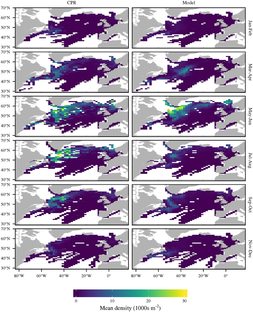
Figure 2. Comparison of bimonthly C. finmarchicus abundance as recorded by CPR and by the model. Density is mean C5 and adult abundance.

FIGURE 3

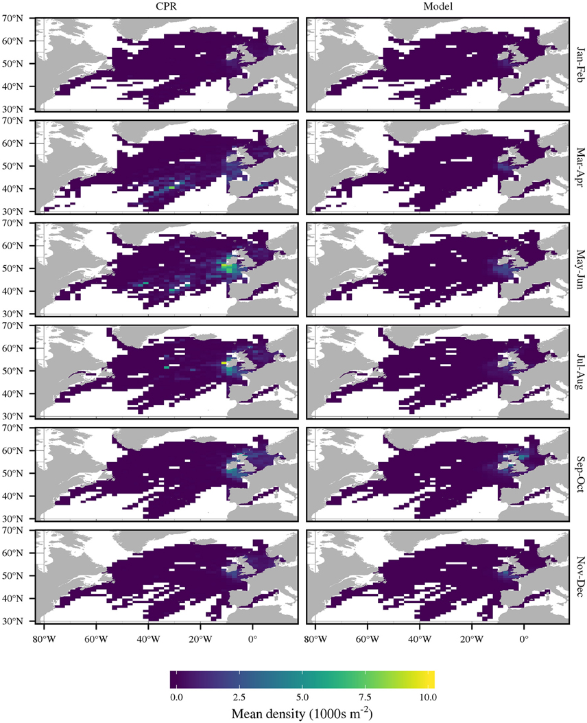
Figure 3. Comparison of bimonthly C. helgolandicus abundance as recorded by CPR and by the model. Density is mean C5 and adult abundance.

TABLE 1

Table 1. The correlation coefficient (r) between modeled monthly abundance and the mean CPR abundance in each cell.

A comparison of bimonthly predictions of C. helgolandicus abundance with the CPR abundance is shown in Figure 3. The correlation coefficient between predicted mean annual abundance and CPR abundance over the 2°E by 1°N cells was 0.76. Importantly, C. helgolandicus was restricted to the continental shelf. The autumn bloom of C. helgolandicus in the North Sea was also reproduced. However, predicted abundance in November and December in the region to the south west of the British Isles appears too high.

Figure 4 shows simulated combined abundance for stage C5 and adult C. finmarchicus compared with those from the time series. Predicted peak abundances are within a factor of 2 of those recorded in the time series, with the exception of the Westmann Islands. OWS I is notable for getting the scale of the first generation very accurate, but we predicted a much larger second generation than is apparent in the time series. We failed to show the apparent sharp increase in C5 and adult at OWS M before day 100. Additionally, the second peak in C5 and adult abundance at OWS M appears to be time shifted by approximately 50 d.

FIGURE 4

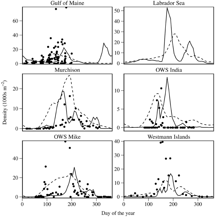
Figure 4. Comparison of modeled C. finmarchicus abundance for combined states C5 and adult with time series data. Solid lines represent model output; dashed lines represent smooths of CPR abundance; points represent time series data. Abundance is depth integrated over the top 100 m of the water column.

We compare predictions for C. helgolandicus with field time series and time series derived from CPR in Figure 5. The timing of the autumn peak of C. helgolandicus abundance at Stonehaven was successfully reproduced. However, we failed to reproduce the small spring bloom. Predicted time and the magnitude of peak abundance was close to that in the L4 time series. However, abundance appeared to be over-predicted during winter.

FIGURE 5

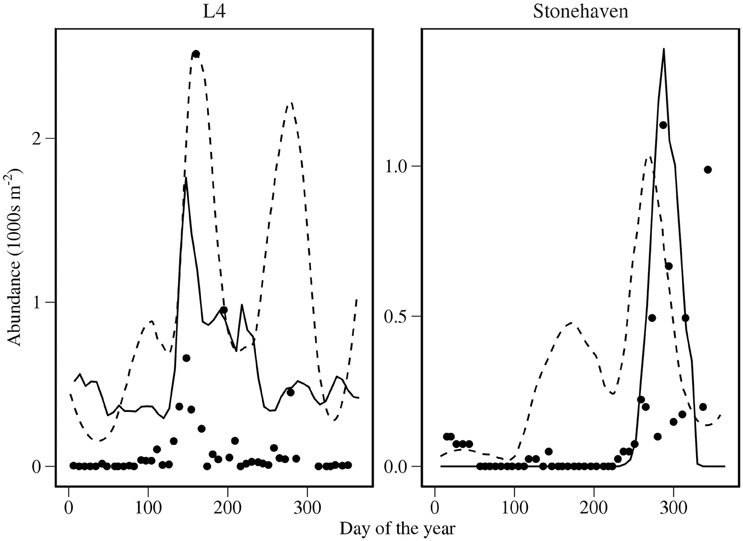
Figure 5. Comparison of modeled abundance of C. helgolandicus for combined states C5 and adult with time series data. Solid lines represent model output; dashed lines represent smooths of CPR abundance; points represent time series data. Abundance is depth integrated over the top 100 m of the water column.

Predicted EPR is compared with field time series at OWS M and L4 for C. finmarchicus and C. helgolandicus respectively in Figure 6. Predicted C. helgolandicus EPR is lower in the first half of the year of the time series, and is slightly time shifted compared with the time series. Predictions depart significantly from the times series in the second half of the year, with EPR being significantly higher than in the time series. The C. finmarchicus EPR time series at OWS M is of short duration. We can therefore only make a limited comparison. However, the predicted EPR is approximately the same as the median EPR in the time series.

FIGURE 6

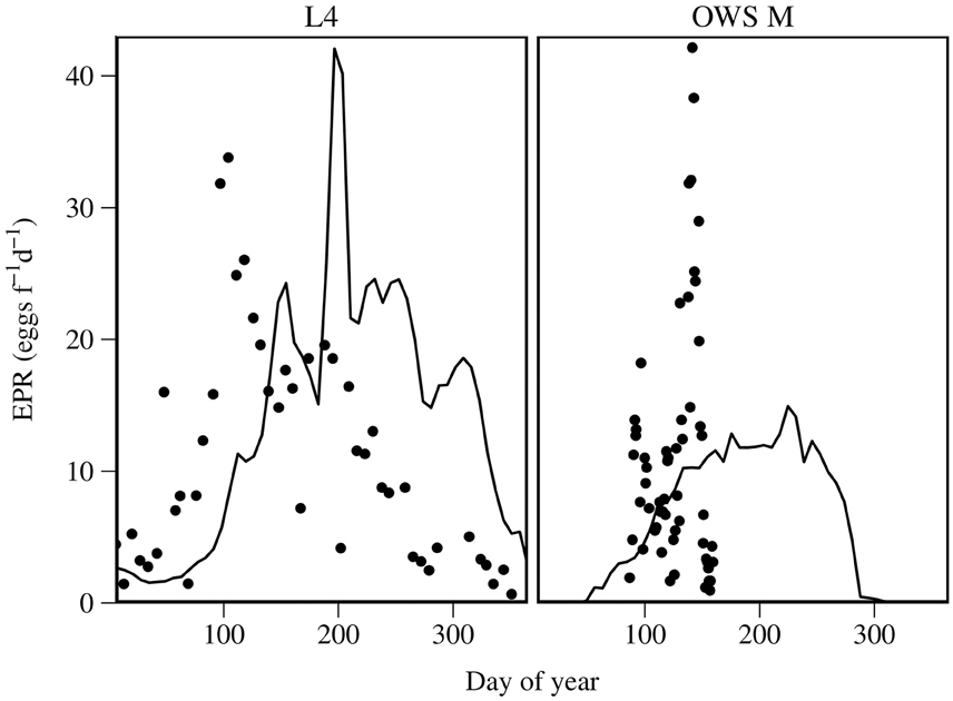
Figure 6. Predicted EPR for C. helgolandicus at L4, English Channel and for C. finmarchicus at OWS M compared with field estimates. Solid lines are modeled EPR; points are field estimates.

3.2. Sensitivity Experiments

In the results shown in Section 3.1, the only differences between the species are the relationship between growth, development and fecundity and temperature, and a parameterized difference in the response of mortality to temperature. Figure 7 shows the predicted geographic distribution of C. finmarchicus when the temperature-dependent mortality parameter for C. helgolandicus was used. The geographic distribution in the west Atlantic is successfully reproduced. However, the geographic distribution in the east Atlantic is too southerly, with a large population predicted to exist in the Celtic Sea.

FIGURE 7

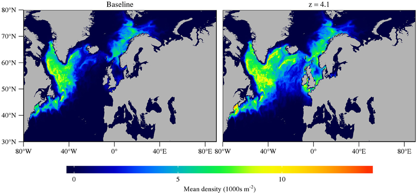
Figure 7. Mean annual abundance of C5 and adult C. finmarchicus under the assumption that temperature scaling of mortality, z = 7 and z = 4.1. A higher value of z means that mortality scales much more steeply with temperature.

Exploratory simulations showed that the C. helgolandicus predictions were sensitive to diapause assumptions. First, the model performed well if C. helgolandicus was assumed to remain at the surface year round and to never diapause. In fact, this simplified model arguably performed better than the original. The key features of the distribution of C. helgolandicus were largely reproduced, with the correlation coefficient (0.78) of model performance compared with CPR actually improving in comparison with our original model.

Further exploratory simulations showed that the state of populations of C. helgolandicus is sensitive to diapause duration. A sensitivity analysis showed that small changes to diapause or mortality assumptions can result in C. helgolandicus becoming an oceanic species. Figure 8 shows the correlation coefficient between predictions and CPR abundance of C. helgolandicus under varying assumptions for diapause duration and the scaling of mortality with temperature. A small reduction in how steeply mortality scales with temperature results in a reduction in model performance, with C. helgolandicus becoming an oceanic species. Likewise, an increase in diapause duration can result in C. helgolandicus becoming an oceanic species. Notably, the high sensitivity to changes in temperature dependent mortality was not evident diapause duration is reduced by 60%, which is potentially a more biologically realistic assumption for diapause duration.

FIGURE 8

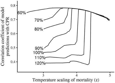
Figure 8. Sensitivity of C. helgolandicus model to diapause duration. Diapause duration was altered by a fixed percentage throughout the model domain, and the temperature scaling of mortality was varied. Abrupt changes in model fit close to the optimum indicates that C. helgolandicus switches from being a shelf to an oceanic species.

4. Discussion

This study can be framed by a single question. What differences between C. finmarchicus and C. helgolandicus explain the relative geographic distributions of these two species? Alternatively, we can ask how much we need to change C. finmarchicus's traits before it effectively becomes C. helgolandicus.

In this setting, the model equations can be viewed as describing a generic Calanus species, while the parameters determine where a species lies in trait space. We showed that the geographic distributions of both species can be reproduced by assuming only two interspecific differences. These were the temperature response of mortality and the temperature influence on ingestion rate, which in turn influences growth, development and fecundity. In other words, we can effectively turn C. finmarchicus into C. helgolandicus by modifying those two traits. This framework has the potential to be applied to a number of Calanus species, and represents a complimentary approach to that taken by others (e.g., Record et al., 2010, 2013; Maps et al., 2012).

A key assumption underlying almost all population models of Calanus is that growth and egg production rate increase monotonically with temperature. This is the second study after Maar et al. (2013) to assume they do not. Instead, we use a dome-shaped relationship between growth and fecundity and temperature. Similar responses have now been established for a number of zooplankton species (White and Roman, 1992; Koski and Kuosa, 1999; Halsband-Lenk et al., 2002; Holste and Peck, 2006; Holste et al., 2009; Rhyne et al., 2009; Pasternak et al., 2013).

The relationships between fecundity and development time and temperature were derived from the experimental ingestion rate data of Møller et al. (2012). A review of the literature shows that we have little knowledge of the key traits of C. finmarchicus such as development, growth and fecundity above 12°C (Table 2). Further, we are not aware of published evidence of the influence of temperature on C. helgolandicus's fecundity. Clarifications of the relationship between growth and temperature are therefore a priority of Calanus research. Importantly, conventional models of development are problematic in the context of climate change, where they may falsely predict ever increasing growth rates as temperatures rise. This is highlighted in the Gulf of Maine, where despite summer surface temperatures now often exceeding 20°C (Mills et al., 2013) there have recently been record high levels of C. finmarchicus abundance (Runge et al., 2014).

TABLE 2

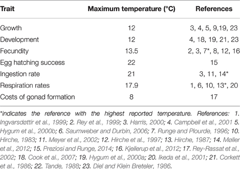
Table 2. Temperature ranges for measurement of key C. finmarchicus traits.

Understanding the relative geographic distributions of both species can arguably be answered by asking why only C. helgolandicus exists in the region south west of the British Isles. On the basis of our models of growth and fecundity, this region is not noticeably favorable to C. helgolandicus. However, the population model's performance is instructive. Simulated abundance of C. helgolandicus is much higher in winter at L4 than in reality, and we significantly over-predicted EPR in the second half of the year compared with the long-term seasonal pattern (Maud et al., 2015). This is potentially related to food quality. Resolving the apparent contradictions in understanding of the influence of food quality on fecundity (Niehoff et al., 1999; Jønasdøttir et al., 2002; Maud et al., 2015) and development time (Diel and Klein Breteler, 1986) may therefore be the key to fully explaining the relative biogeographies of both species.

Measuring mortality in copepods is commonly viewed as an intractable problem (Ohman, 2012), and therefore models of mortality are inherently uncertain and difficult to validate. This problem is highlighted by our formulation of starvation mortality, where it was related to growth rate. The formulation was similar to that used by other modelers (e.g., Tittensor et al., 2003), however it was ad-hoc and impossible to validate. Importantly, the modeled biogeography of C. helgolandicus was dependent on starvation mortality, where it plays a key role in reducing post-diapause populations in oceanic regions to a low enough level to eliminate long-term persistence. However, alternative formulations of mortality could potentially achieve this. Some zooplankton modelers have used U-shaped relationships between mortality and temperature (Rajakaruna et al., 2012), which could act as a limit on the north-western distribution of C. helgolandicus. Further, allee effects (Kiørboe, 2006) and the impact of starvation on long-term fecundity (Niehoff, 2004) could significantly deplete the populations of low-abundance post-diapause C. helgolandicus populations. Including these mortality effects in our model would result in a more complete representation of copepod ecology. However, there is little evidence to quantify the relative magnitude of these sources of mortality. Further advances in understanding copepod mortality (Gentleman et al., 2012; Ohman, 2012) are therefore likely necessary to justify increasingly complex mortality models. However, the influence of mortality should be considered if the model is to be applied, particularly in climate change contexts where changes might be dependent on the specific mortality formulation.

There is a spring bloom of C. helgolandicus in the North Sea (Bresnan et al., 2015), which we did not predict. However, the apparent phenology of C. helgolandicus in the North Sea is difficult to reconcile with the known influence of temperature on its development time (Cook et al., 2007; Bonnet et al., 2009). The first Stonehaven bloom typically occurs before day 130, and temperatures are below 9 °C before then. Evidence indicates that C. helgolandicus either cannot develop from egg to adult (Bonnet et al., 2009) or has a development time greater than 120 d at these temperatures (Møller et al., 2012). Research is therefore needed to reconcile development time studies of C. helgolandicus and phenology in the North Sea. Further, additional model runs (not shown) indicated that most of the modeled autumn bloom in the northern North Sea resulted from animals that are advected into the North Sea from the North. The importance of advection for North Sea C. finmarchicus populations has been previously been studied (Heath et al., 1999), however the role of advection in influencing year to year North Sea C. helgolandicus abundance has not. It may be possible that C. helgolandicus phenology in the North Sea can be explained by the existence of hybrids of C. helgolandicus and C. finmarchicus. This is a speculative hypothesis. However, at the fringes of its northern distribution, C. finmarchicus hybridizes with C. glacialis (Parent et al., 2011; Gabrielsen et al., 2012; Berchenko and Stupnikova, 2014), and we cannot rule out a similar phenomenon for C. finmarchicus and C. helgolandicus.

Finally, our model highlights the importance of lipid dynamics and deep-water temperatures as influences on the distribution of Calanus. Existing statistical models of Calanus biogeography (Helaouët and Beaugrand, 2007; Chust et al., 2013; Hinder et al., 2013) and projections of future distributions (Reygondeau and Beaugrand, 2011; Villarino et al., 2015) have only considered surface conditions. However, the distribution of C. helgolandicus appears to be strongly influenced by deep-water temperatures. Conditions in large parts of the North Atlantic are sufficient to support at least one generation of C. helgolandicus, but high overwintering temperatures result in the inability of a sufficiently large overwintering population to maintain a persistent population. Recent work showed that projected potential diapause duration of C. finmarchicus in the Norwegian Sea under a high emissions scenario was largely unchanged this century, whereas surface temperature increases significantly (Wilson et al., 2016). Development conditions will therefore improve significantly for C. helgolandicus in the Norwegian Sea, whereas diapause conditions would remain largely unchanged. There is therefore potential for C. helgolandicus to become an oceanic species as a result of deep-water warming lagging that at the surface. Similarly, these marginal changes in potential diapause duration may act as a brake on the northward retreat of C. finmarchicus. However, the expected temperature increases across the North Atlantic will reduce lipid levels of animals (Wilson et al., 2016) and the consequences are poorly understood. The future evolution of lipid dynamics may therefore be pivotal in determining the fate of Calanus communities and will have important consequences for the fish, seabirds and marine mammals that depend on the lipids provided by copepods (Beaugrand and Kirby, 2010; Frederiksen et al., 2013).

Author Contributions

RW, MH, and DS contributed to the design of the model. RW implemented and analyzed the model and led the writing of the paper. All authors contributed to the editing and refining of the paper.

Funding

This work received funding from the MASTS pooling initiative (The Marine Alliance for Science and Technology for Scotland) and their support is gratefully acknowledged. MASTS is funded by the Scottish Funding Council (grant reference HR09011) and contributing institutions.

Conflict of Interest Statement

The authors declare that the research was conducted in the absence of any commercial or financial relationships that could be construed as a potential conflict of interest.

Acknowledgments

We thank the Continuous Plankton Recorder Survey for providing access to data, and Neil Banas for fruitful discussions that helped shape the diapause model in the paper. Andrew Yool provided output from the NEMO model. Nicholas Record and a second reviewer provided helpful critical comments which improved the manuscript. Finally, we thank Ian Thurlbeck for invaluable IT support.

Supplementary Material

The Supplementary Material for this article can be found online at: https://www.frontiersin.org/article/10.3389/fmars.2016.00157

References

Barton, A. D., Pershing, A. J., Litchman, E., Record, N. R., Edwards, K. F., Finkel, Z. V., et al. (2013). The biogeography of marine plankton traits. Ecol. Lett. 16, 522–534. doi: 10.1111/ele.12063

PubMed Abstract | CrossRef Full Text | Google Scholar

Batten, S. D., Clark, R., Flinkman, J., Hays, G., John, E., John, A. W. G., et al. (2003). CPR sampling: the technical background, materials and methods, consistency and comparability. Prog. Oceanogr. 58, 193–215. doi: 10.1016/j.pocean.2003.08.004

CrossRef Full Text | Google Scholar

Beaugrand, G. (2012). Unanticipated biological changes and global warming. Mar. Ecol. Prog. Ser. 445, 293–301. doi: 10.3354/meps09493

CrossRef Full Text | Google Scholar

Beaugrand, G., and Kirby, R. R. (2010). Climate, plankton and cod. Global Change Biol. 16, 1268–1280. doi: 10.1111/j.1365-2486.2009.02063.x

CrossRef Full Text | Google Scholar

Beaugrand, G., Luczak, C., and Edwards, M. (2009). Rapid biogeographical plankton shifts in the North Atlantic Ocean. Global Change Biol. 15, 1790–1803. doi: 10.1111/j.1365-2486.2009.01848.x

CrossRef Full Text | Google Scholar

Beaugrand, G., Reid, P. C., Ibañez, F., Lindley, J. A., and Edwards, M. (2002). Reorganization of North Atlantic marine copepod biodiversity and climate. Science 296, 1692–1694. doi: 10.1126/science.1071329

PubMed Abstract | CrossRef Full Text | Google Scholar

Berchenko, I. V., and Stupnikova, A. N. (2014). Morphological peculiarities of Calanus finmarchicus and Calanus glacialis in the areas of the co-existence of their populations. Oceanology 54, 450–457. doi: 10.1134/S0001437014040031

CrossRef Full Text | Google Scholar

Bonnet, D., Harris, R. P., Yebra, L., Guilhaumon, F., Conway, D. V. P., and Hirst, A. G. (2009). Temperature effects on Calanus helgolandicus (Copepoda: Calanoida) development time and egg production. J. Plankton Res. 31, 31–44. doi: 10.1093/plankt/fbn099

CrossRef Full Text | Google Scholar

Bonnet, D., Richardson, A., Harris, R., Hirst, A., Beaugrand, G., Edwards, M., et al. (2005). An overview of Calanus helgolandicus ecology in European waters. Prog. Oceanogr. 65, 1–53. doi: 10.1016/j.pocean.2005.02.002

CrossRef Full Text | Google Scholar

Bresnan, E., Cook, K. B., Hughes, S. L., Hay, S. J., Smith, K., Walsham, P., et al. (2015). Seasonality of the plankton community at an east and west coast monitoring site in Scottish waters. J. Sea Res. 105, 16–29. doi: 10.1016/j.seares.2015.06.009

CrossRef Full Text | Google Scholar

Campbell, R. G., Wagner, M. M., Teegarden, G. J., Boudreau, C. A., and Durbin, E. G. (2001). Growth and development rates of Calanus finmarchicus the copepod reared in the laboratory. Mar. Ecol. Prog. Ser. 221, 161–183. doi: 10.3354/meps221161

CrossRef Full Text

Chust, G., Castellani, C., Licandro, P., Ibaibarriaga, L., Sagarminaga, Y., and Irigoien, X. (2013). Are Calanus spp. shifting poleward in the North Atlantic? A habitat modelling approach. ICES J. Mar. Sci. 71, 241–253. doi: 10.1093/icesjms/fst147

CrossRef Full Text | Google Scholar

Clarke, E. D., Speirs, D. C., Heath, M., Wood, S. N., Gurney, W. S. C., and Holmes, S. J. (2006). Calibrating remotely sensed chlorophyll-a data by using penalized regression splines. J. R. Stat. Soc. Ser. C 55, 331–353. doi: 10.1111/j.1467-9876.2006.00540.x

CrossRef Full Text | Google Scholar

Comiso, J. (1997). Bootstrap Sea Ice Concentrations from Nimbus-7 SMMR and DMSP SSM/I-SSMIS. Boulder, CO: Natinoal Snow and Ice Data Center.

Cook, K. B., Bunker, A., Hay, S., Hirst, A. G., and Speirs, D. C. (2007). Naupliar development times and survival of the copepods Calanus helgolandicus and Calanus finmarchicus in relation to food and temperature. J. Plankton Res. 29, 757–767. doi: 10.1093/plankt/fbm056

CrossRef Full Text | Google Scholar

Corkett, C. J., McLaren, I. A., and Sevigny, J.-M. (1986). The rearing of the marine calanoid copepods Calanus finmarchicus (Gunnerus), C. glacialis Jaschnov and C. hyperboreus Krøyer with comment on the equiproportional rule. Syllogeus 58, 539–546.

Diel, S., and Klein Breteler, W. C. M. (1986). Growth and development of Calanus spp. (Copepoda) during spring phytoplankton succession in the North Sea. Mar. Biol. 92, 85–92. doi: 10.1007/BF00397574

CrossRef Full Text | Google Scholar

Durbin, E. G., Garrahan, P. R., and Casas, M. C. (2000). Abundance and distribution of Calanus finmarchicus on the Georges Bank during 1995 and 1996. ICES J. Mar. Sci. 57, 1664–1685. doi: 10.1006/jmsc.2000.0974

CrossRef Full Text | Google Scholar

Eiane, K., Aksnes, D. L., Ohman, M. D., Wood, S., and Martinussen, M. B. (2002). Stage-specific mortality of Calanus spp. under different predation regimes. Sarsia 47, 636–645. doi: 10.4319/lo.2002.47.3.0636

CrossRef Full Text | Google Scholar

Frederiksen, M., Anker-Nilssen, T., Beaugrand, G., and Wanless, S. (2013). Climate, copepods and seabirds in the boreal Northeast Atlantic - current state and future outlook. Global Change Biol. 19, 364–372. doi: 10.1111/gcb.12072

CrossRef Full Text

Gabrielsen, T. M., Merkel, B., Sreide, J. E., Johansson-Karlsson, E., Bailey, A., Vogedes, D., et al. (2012). Potential misidentifications of two climate indicator species of the marine arctic ecosystem: Calanus glacialis and C. finmarchicus. Polar Biol. 35, 1621–1628. doi: 10.1007/s00300-012-1202-7

CrossRef Full Text | Google Scholar

Gentleman, W. C., Pepin, P., and Doucette, S. (2012). Estimating mortality: clarifying assumptions and sources of uncertainty in vertical methods. J. Mar. Syst. 105–108, 1–19. doi: 10.1016/j.jmarsys.2012.05.006

CrossRef Full Text | Google Scholar

Gislason, A., and Astthorsson, O. S. (2000). Winter distribution, ontogenetic migration, and rates of egg production of Calanus finmarchicus southwest of Iceland. ICES J. Mar. Sci. 57, 1727–1739. doi: 10.1006/jmsc.2000.0951

CrossRef Full Text | Google Scholar

Gurney, W. S. C., Speirs, D. C., Wood, S. N., Clarke, E. D., and Heath, M. R. (2001). Simulating spatially and physiologically structured populations. J. Anim. Ecol. 70, 881–894. doi: 10.1046/j.0021-8790.2001.00549.x

CrossRef Full Text | Google Scholar

Halsband-Lenk, C., Hirche, H.-J., and Carlotti, F. (2002). Temperature impact on reproduction and development of congener copepod populations. J. Exp. Mar. Biol. Ecol. 271, 121–153. doi: 10.1016/S0022-0981(02)00025-4

CrossRef Full Text | Google Scholar

Harris, R. (2000). Feeding, growth, and reproduction in the genus Calanus. ICES J. Mar. Sci. 57, 1708–1726. doi: 10.1006/jmsc.2000.0959

CrossRef Full Text | Google Scholar

Harris, R. (2010). The L4 time-series: the first 20 years. J. Plankton Res. 32, 577–583. doi: 10.1093/plankt/fbq021

CrossRef Full Text | Google Scholar

Heath, M. R., Astthorsson, O. S., Dunn, J., Ellertsen, B., Gaard, E., Gislason, A., et al. (2000). Comparative analysis of Calanus finmarchicus demography at locations around the Northeast Atlantic. ICES J. Mar. Sci. 57, 1562–1580. doi: 10.1006/jmsc.2000.0950

CrossRef Full Text | Google Scholar

Heath, M. R., Backhaus, J. O., Richardson, K., McKenzie, E., Slagstad, D., Beare, D., et al. (1999). Climate fluctuations and the spring invasion of the North Sea by Calanus finmarchicus. Fish. Oceanogr. 8, 163–176. doi: 10.1046/j.1365-2419.1999.00008.x

CrossRef Full Text | Google Scholar

Heath, M. R., Boyle, P., Gislason, A., Gurney, W. S. C., Hay, S. J., Head, E. J. H., et al. (2004). Comparative ecology of over-wintering Calanus finmarchicus in the northern North Atlantic, and implications for life-cycle patterns. ICES J. Mar. Sci. 61, 698–708. doi: 10.1016/j.icesjms.2004.03.013

CrossRef Full Text | Google Scholar

Helaouët, P., and Beaugrand, G. (2007). Macroecology of Calanus finmarchicus and C. helgolandicus in the North Atlantic Ocean and adjacent seas. Mar. Ecol. Prog. Ser. 345, 147–165. doi: 10.3354/meps06775

CrossRef Full Text | Google Scholar

Hélaouët, P., Beaugrand, G., and Reygondeau, G. (2016). Reliability of spatial and temporal patterns of C. finmarchicus inferred from the CPR survey. J. Mar. Syst. 153, 18–24. doi: 10.1016/j.jmarsys.2015.09.001

CrossRef Full Text | Google Scholar

Hinder, S. L., Gravenor, M. B., Edwards, M., Ostle, C., Bodger, O. G., Lee, P. L. M., et al. (2013). Multi-decadal range changes vs. thermal adaptation for north east Atlantic oceanic copepods in the face of climate change. Global Change Biol. 20, 140–146. doi: 10.1111/gcb.12387

PubMed Abstract | CrossRef Full Text | Google Scholar

Hirche, H.-J. (1983). Overwintering of Calanus finmarchicus and Calanus helgolandicus. Mar. Ecol. Prog. Ser. 11, 281–290. doi: 10.3354/meps011281

CrossRef Full Text | Google Scholar

Hirche, H.-J. (1987). Temperature and plankton II. Effect on respiration and swimming activity in copepods from the Greenland Sea. Mar. Biol. 95, 347–356. doi: 10.1007/BF00428240

CrossRef Full Text | Google Scholar

Hirche, H.-J., Brey, T., and Niehoff, B. (2001). A high-frequency time series at Ocean Weather Ship Station M (Norwegian Sea): population dynamics of Calanus finmarchicus. Mar. Ecol. Prog. Ser. 219, 205–219. doi: 10.3354/meps219205

CrossRef Full Text | Google Scholar

Hirche, H.-J., Meyer, U., and Niehoff, B. (1997). Egg production of Calanus finmarchicus: effect of temperature, food and season. Mar. Biol. 127, 609–620. doi: 10.1007/s002270050051

CrossRef Full Text | Google Scholar

Hirst, A. G., Bonnet, D., and Harris, R. P. (2007). Seasonal dynamics and mortality rates of Calanus helgolandicus over two years at a station in the English Channel. Mar. Ecol. Prog. Ser. 340, 189–205. doi: 10.3354/meps340189

CrossRef Full Text | Google Scholar

Holste, L., and Peck, M. A. (2006). The effects of temperature and salinity on egg production and hatching success of Baltic Acartia tonsa (Copepoda: Calanoida): a laboratory investigation. Mar. Biol. 148, 1061–1070. doi: 10.1007/s00227-005-0132-0

CrossRef Full Text | Google Scholar

Holste, L., St. John, M. A., and Peck, M. A. (2009). The effects of temperature and salinity on reproductive success of Temora longicornis in the Baltic Sea: a copepod coping with a tough situation. Mar. Biol. 156, 527–540. doi: 10.1007/s00227-008-1101-1

CrossRef Full Text | Google Scholar

Hygum, B. H., Rey, C., and Hansen, B. W. (2000a). Growth and development rates of Calanus finmarchicus nauplii during a diatom spring bloom. Mar. Biol. 136, 1075–1085. doi: 10.1007/s002270000313

CrossRef Full Text | Google Scholar

Hygum, B. H., Rey, C., Hansen, B. W., and Tande, K. (2000b). Importance of food quantity to structural growth rate and neutral lipid reserves accumulated in Calanus finmarchicus. Mar. Biol. 136, 1057–1073. doi: 10.1007/s002270000292

CrossRef Full Text | Google Scholar

Ikeda, T., Kanno, Y., Ozaki, K., and Shinada, A. (2001). Metabolic rates of epipelagic marine copepods as a function of body mass and temperature. Mar. Biol. 139, 587–596. doi: 10.1007/s002270100608

CrossRef Full Text | Google Scholar

Ingvarsdøttir, A., Houlihan, D. F., Heath, M. R., and Hay, S. J. (1999). Seasonal changes in respiration rates of copepodite stage V Calanus finmarchicus (Gunnerus). Fish. Oceanogr. 8, 73–83. doi: 10.1046/j.1365-2419.1999.00002.x

CrossRef Full Text | Google Scholar

Irigoien, X. (1999). Vertical distribution and population structure of Calanus fimarchicus at station India (59 °N, 19 °W) during the passage of the great salinity anomaly, 1971-1975. Deep Sea Res. I 47, 1–26. doi: 10.1016/S0967-0637(99)00045-X

CrossRef Full Text

Irigoien, X., Head, R. N., Harris, R. P., Cummings, D., and Harbour, D. (2000). Feeding selectivity and egg production of Calanus helgolandicus in the English Channel. Limnol. Oceanogr. 45, 44–54. doi: 10.4319/lo.2000.45.1.0044

CrossRef Full Text | Google Scholar

Jønasdøttir, S. H., Gudfinnsson, H. G., Gislason, A., and Astthorsson, O. S. (2002). Diet composition and quality for Calanus finmarchicus egg production and hatching success off south-west Iceland. Mar. Biol. 140, 1195–1206. doi: 10.1007/s00227-002-0782-0

CrossRef Full Text | Google Scholar

Kiørboe, T. (2006). Sex, sex-ratios, and the dynamics of pelagic copepod populations. Oecologia 148, 40–50. doi: 10.1007/s00442-005-0346-3

PubMed Abstract | CrossRef Full Text | Google Scholar

Kjellerup, S., Dünweber, M., Swalethorp, R., Nielsen, T. G., Møller, E. F., Markager, S., et al. (2012). Effects of a future warmer ocean on the coexisting copepods Calanus finmarchicus and C. glacialis in Disko Bay, western Greenland. Mar. Ecol. Prog. Ser. 447, 87–108. doi: 10.3354/meps09551

CrossRef Full Text | Google Scholar

Koski, M., and Kuosa, H. (1999). The effect of temperature, food concentration and female size on the egg production of the planktonic copepod Acartia bifilosa. J. Plankton Res. 21, 1779–1789. doi: 10.1093/plankt/21.9.1779

CrossRef Full Text | Google Scholar

Lett, C., Verley, P., Mullon, C., Parada, C., Brochier, T., Penven, P., et al. (2008). A Lagrangian tool for modelling ichthyoplankton dynamics. Environ. Model. Softw. 23, 1210–1214. doi: 10.1016/j.envsoft.2008.02.005

CrossRef Full Text | Google Scholar

Litchman, E., Ohman, M. D., and Kiørboe, T. (2013). Trait-based approaches to zooplankton communities. J. Plankton Res. 35, 473–484. doi: 10.1093/plankt/fbt019

CrossRef Full Text | Google Scholar

Maar, M., Møller, E. F., Gürkan, Z., Jønasdøttir, S. H., and Nielsen, T. G. (2013). Sensitivity of Calanus spp. copepods to environmental changes in the North Sea using life-stage structured models. Prog. Oceanogr. 111, 24–37. doi: 10.1016/j.pocean.2012.10.004

CrossRef Full Text | Google Scholar

Madec, G. (2012). “NEMO ocean engine,” in Note du Pole de modélisation, Institut Pierre-Simon Laplace (IPSL) (Paris).

Maps, F., Pershing, A. J., and Record, N. R. (2012). A generalized approach for simulating growth and development in diverse marine copepod species. ICES J. Mar. Sci. 69, 370–379. doi: 10.1093/icesjms/fsr182

CrossRef Full Text | Google Scholar

Maud, J. L., Atkinson, A., Hirst, A. G., Lindeque, P. K., Widdicombe, C. E., Harmer, R. A., et al. (2015). How does Calanus helgolandicus maintain its population in a variable environment? Analysis of a 25-year time series from the English Channel. Prog. Oceanogr. 137, 513–523. doi: 10.1016/j.pocean.2015.04.028

CrossRef Full Text | Google Scholar

McLaren, I. A., and Leonard, A. (1995). Assessing the equivalence of growth and egg production of copepods. ICES J. Mar. Sci. 52, 397–408. doi: 10.1016/1054-3139(95)80055-7

CrossRef Full Text | Google Scholar

Melle, W., Runge, J., Head, E., Plourde, S., Castellani, C., Licandro, P., et al. (2014). The North Atlantic Ocean as habitat for Calanus finmarchicus: environmental factors and life history traits. Prog. Oceanogr. 129, 244–284. doi: 10.1016/j.pocean.2014.04.026

CrossRef Full Text | Google Scholar

Meyer, B., Irigoien, X., Graeve, M., Head, R. N., and Harris, R. P. (2002). Feeding rates and selectivity among nauplii, copepodites and adult females of Calanus finmarchicus and Calanus helgolandicus. Helgoland Mar. Res. 56, 169–176. doi: 10.1007/s10152-002-0105-3

CrossRef Full Text | Google Scholar

Mills, K., Pershing, A., and Brown, C. (2013). Fisheries management in a changing climate: lessons from the 2012 ocean heat wave in the northwest Atlantic. Oceanography 26, 191–195. doi: 10.5670/oceanog.2013.27

CrossRef Full Text | Google Scholar

Møller, E. F., Maar, M., Jónasdóttir, S. H., Gissel Nielsen, T., and Tönnesson, K. (2012). The effect of changes in temperature and food on the development of Calanus finmarchicus and Calanus helgolandicus populations. Limnol. Oceanogr. 57, 211–220. doi: 10.4319/lo.2012.57.1.0211

CrossRef Full Text | Google Scholar

Niehoff, B. (2004). The effect of food limitation on gonad development and egg production of the planktonic copepod Calanus finmarchicus. J. Exp. Mar. Biol. Ecol. 307, 237–259. doi: 10.1016/j.jembe.2004.02.006

CrossRef Full Text | Google Scholar

Niehoff, B., Klenke, U., Hirche, H. J., Irigoien, X., Head, R., and Harris, R. (1999). A high frequency time series at Weathership M, Norwegian Sea, during the 1997 spring bloom: the reproductive biology of Calanus finmarchicus. Mar. Ecol. Prog. Ser. 176, 81–92. doi: 10.3354/meps176081

CrossRef Full Text | Google Scholar

Ohman, M. D. (2012). Estimation of mortality for stage-structured zooplankton populations: what is to be done? J. Mar. Syst. 93, 4–10. doi: 10.1016/j.jmarsys.2011.05.008

CrossRef Full Text | Google Scholar

Ohman, M. D., Eiane, K., Durbin, E. G., Runge, J. A., and Hirche, H. J. (2004). A comparative study of Calanus finmarchicus mortality patterns at five localities in the North Atlantic. ICES J. Mar. Sci. 61, 687–697. doi: 10.1016/j.icesjms.2004.03.016

CrossRef Full Text | Google Scholar

Parent, G. J., Plourde, S., and Turgeon, J. (2011). Overlapping size ranges of Calanus spp. off the Canadian Arctic and Atlantic Coasts: impact on species' abundances. J. Plankt. Res. 33, 1654–1665. doi: 10.1093/plankt/fbr072

CrossRef Full Text | Google Scholar

Parent, G. J., Plourde, S., and Turgeon, J. (2012). Natural hybridization between Calanus finmarchicus and C. glacialis (Copepoda) in the Arctic and Northwest Atlantic. Limnol. Oceanogr. 57, 1057–1066. doi: 10.4319/lo.2012.57.4.1057

CrossRef Full Text | Google Scholar

Parsons, T. R., Takahashi, M., and Hargrave, B. (1984). Biological Oceanographic Processes. Oxford: Pergamon Press.

Google Scholar

Pasternak, A. F., Arashkevich, E. G., Grothe, U., Nikishina, A. B., and Solovyev, K. A. (2013). Different effects of increased water temperature on egg production of Calanus finmarchicus and C. glacialis. Mar. Biol. 53, 547–553. doi: 10.1134/s0001437013040085

CrossRef Full Text | Google Scholar

Planque, B., and Batten, S. D. (2000). Calanus finmarchicus in the North Atlantic: the year of Calanus in the context of interdecadal change. ICES J. Mar. Sci. 57, 1528–1535. doi: 10.1006/jmsc.2000.0970

CrossRef Full Text | Google Scholar

Preziosi, B. M., and Runge, J. A. (2014). The effect of warm temperatures on hatching success of the marine planktonic copepod, Calanus finmarchicus. J. Plankton Res. 36, 1381–1384. doi: 10.1093/plankt/fbu056

CrossRef Full Text | Google Scholar

Rae, K. S. M. (1952). Continuous plankton records: explanation and methods, 1946-1949. Bull. Mar. Ecol. 3, 135–155.

Rajakaruna, H., Strasser, C., and Lewis, M. (2012). Identifying non-invasible habitats for marine copepods using temperature-dependent R 0. Biol. Invas. 14, 633–647. doi: 10.1007/s10530-011-0104-x

CrossRef Full Text | Google Scholar

Record, N. R., and Pershing, A. J. (2008). Modeling zooplankton development using the monotonic upstream scheme for conservation laws. Limnol. Oceanogr. Methods 6, 364–373. doi: 10.4319/lom.2008.6.364

CrossRef Full Text | Google Scholar

Record, N. R., Pershing, A. J., and Maps, F. (2013). Emergent copepod communities in an adaptive trait-structured model. Ecol. Model. 260, 11–24. doi: 10.1016/j.ecolmodel.2013.03.018

CrossRef Full Text | Google Scholar

Record, N. R., Pershing, A. J., Runge, J. A., Mayo, C. A., Monger, B. C., and Chen, C. (2010). Improving ecological forecasts of copepod community dynamics using genetic algorithms. J. Mar. Syst. 82, 96–110. doi: 10.1016/j.jmarsys.2010.04.001

CrossRef Full Text | Google Scholar

Reid, P. C., Edwards, M., Beaugrand, G., Skogen, M., and Stevens, D. (2003). Periodic changes in the zooplankton of the North Sea during the twentieth century linked to oceanic inflow. Fish. Oceanogr. 12, 260–269. doi: 10.1046/j.1365-2419.2003.00252.x

CrossRef Full Text | Google Scholar

Rey, C., Carlotti, F., Tande, K., and Hansen, B. H. (1999). Egg and faecal pellet production of Calanus finmarchicus females from controlled mesocosms and in situ populations: influence of age and feeding history. Mar. Ecol. Prog. Ser. 188, 133–148. doi: 10.3354/meps188133

CrossRef Full Text | Google Scholar

Rey-Rassat, C., Irigoien, X., Harris, R., and Carlotti, F. (2002). Energetic cost of gonad development in Calanus finmarchicus and C. helgolandicus. Mar. Ecol. Prog. Ser. 238, 301–306. doi: 10.3354/meps238301

CrossRef Full Text | Google Scholar

Reygondeau, G., and Beaugrand, G. (2011). Future climate-driven shifts in distribution of Calanus finmarchicus. Global Change Biol. 17, 756–766. doi: 10.1111/j.1365-2486.2010.02310.x

CrossRef Full Text | Google Scholar

Rhyne, A. L., Ohs, C. L., and Stenn, E. (2009). Effects of temperature on reproduction and survival of the calanoid copepod Pseudodiaptomus pelagicus. Aquaculture 292, 53–59. doi: 10.1016/j.aquaculture.2009.03.041

CrossRef Full Text | Google Scholar

Richardson, A. J., Walne, A. W., John, A. W. G., Jonas, T. D., Lindley, J. A., Sims, D. W., et al. (2006). Using Continuous Plankton Recorder data. Prog. Oceanogr. 68, 27–74. doi: 10.1016/j.pocean.2005.09.011

CrossRef Full Text | Google Scholar

Runge, J. A., Ji, R., Thompson, C. R. S., Record, N. R., Chen, C., Vandemark, D. C., et al. (2014). Persistence of Calanus finmarchicus in the western Gulf of Maine during recent extreme warming. J. Plank. Res. 37, 221–232. doi: 10.1093/plankt/fbu098

CrossRef Full Text | Google Scholar

Runge, J. A., and Plourde, S. (1996). Fecundity characteristics of Calanus finmarchicus in coastal waters of eastern Canada. Ophelia 44, 171–187. doi: 10.1080/00785326.1995.10429846

CrossRef Full Text | Google Scholar

Saumweber, W. J., and Durbin, E. G. (2006). Estimating potential diapause duration in Calanus finmarchicus. Deep Sea Res. II 53, 2597–2617. doi: 10.1016/j.dsr2.2006.08.003

CrossRef Full Text | Google Scholar

Speirs, D. C., Gurney, W. S. C., Heath, M. R., Horbelt, W., Wood, S. N., and de Cuevas, B. A. (2006). Ocean-scale modelling of the distribution, abundance, and seasonal dynamics of the copepod Calanus finmarchicus. Mar. Ecol. Prog. Ser. 313, 173–192. doi: 10.3354/meps313173

CrossRef Full Text | Google Scholar

Speirs, D. C., Gurney, W. S. C., Heath, M. R., and Wood, S. N. (2005). Modelling the basin-scale demography of Calanus finmarchicus in the north-east Atlantic. Fish. Oceanogr. 14, 333–358. doi: 10.1111/j.1365-2419.2005.00339.x

CrossRef Full Text | Google Scholar

Tande, K. S. (1988). Aspects of developmental and mortality rates in Calanus finmarchicus related to equiproportional development. Mar. Ecol. Prog. Ser. 44, 51–58. doi: 10.3354/meps044051

CrossRef Full Text | Google Scholar

Tittensor, D. P., Deyoung, B., and Tang, C. L. (2003). Modelling the distribution, sustainability and diapause emergence timing of the copepod Calanus finmarchicus in the Labrador Sea. Fish. Oceanogr. 12, 299–316. doi: 10.1046/j.1365-2419.2003.00266.x

CrossRef Full Text | Google Scholar

Villarino, E., Chust, G., Licandro, P., Butenschön, M., Ibaibarriaga, L., Larrañaga, A., et al. (2015). Modelling the future biogeography of North Atlantic zooplankton communities in response to climate change. Mar. Ecol. Prog. Ser. 531, 121–142. doi: 10.3354/meps11299

CrossRef Full Text | Google Scholar

White, J. R., and Roman, M. R. (1992). Egg production by the calanoid copepod Acartia tonsa in the mesohaline Chesapeake Bay: the importance of food resources and temperature. Mar. Ecol. Prog. Ser. 86, 239–249. doi: 10.3354/meps086239

CrossRef Full Text | Google Scholar

Wilson, R. J., Banas, N. S., Heath, M. R., and Speirs, D. C. (2016). Projected impacts of 21st century climate change on diapause in Calanus finmarchicus. Glob. Chang. Biol. 22, 3332–3340. doi: 10.1111/gcb.13282

PubMed Abstract | CrossRef Full Text | Google Scholar

Wilson, R. J., Speirs, D. C., and Heath, M. R. (2015). On the surprising lack of differences between two congeneric calanoid copepod species, Calanus finmarchicus and C. helgolandicus. Prog. Oceanogr. 134, 413–431. doi: 10.1016/j.pocean.2014.12.008

CrossRef Full Text | Google Scholar

Yool, A., Popova, E. E., and Anderson, T. R. (2011). Medusa-1.0: a new intermediate complexity plankton ecosystem model for the global domain. Geosci. Model Dev. 4, 381–417. doi: 10.5194/gmd-4-381-2011

CrossRef Full Text | Google Scholar