Modeling the Potential Distribution and Richness of Cetaceans in the Azores from Fisheries Observer Program Data

Introduction

The world's oceans face increasing pressure from anthropogenic influences (Halpern et al., 2008). As a result, the rate of change in distribution and population fragmentation of marine organisms has intensified over the last few decades, upsetting the equilibrium of marine ecosystems (Pitois and Fox, 2006; Worm et al., 2006; Beaugrand, 2009; Poloczanska et al., 2013).

Marine mammals (of which cetaceans comprise nearly 70% of the extant species) are especially affected by changes in marine ecosystems and by human threats, with an estimated 74% of species facing high levels of human impact (Davidson et al., 2012; Bester, 2014). Being large-sized top predators with a high metabolic rate, cetaceans play an important role in maintaining the structure and functioning of the marine ecosystems they integrate (Bowen, 1997; Roman et al., 2014; Kiszka et al., 2015).

Cetaceans are expected to experience important changes in distribution due to direct effects of climate change and in response to climactic- and anthropogenic-driven reorganization of their ecosystems (Learmonth et al., 2006; Simmonds and Isaac, 2007; Moore and Huntington, 2008; Bester, 2014). For example, drastic changes in seawater temperature are expected to affect the geographical distribution of species with narrow thermal tolerance, such as some species that occur only in the Arctic or tropical species (Learmonth et al., 2006; Simmonds and Eliott, 2009). In fact, Salvadeo et al. (2010) proposed that a decline in the presence of Pacific white-sided dolphins (Lagenorhynchus obliquidens) in the southwest Gulf of California could be explained by a consistent increase in water temperature in that region over three decades. Similarly, MacLeod et al. (2005) reported a decline of the relative frequencies of strandings and sightings of white-beaked dolphins (Lagenorhynchus albirostris) and a simultaneous relative increase in the strandings and sightings of the common dolphin (Delphinus delphis) in the northwest Scotland shelf and suggested that these changes could be due to distributional shift of the two species, driven by a steady increase in water temperature.

Distribution and abundance shifts of potential cetacean prey have also been recorded in some areas (e.g., Hátún et al., 2009; Chust et al., 2014; Cormon et al., 2014). Changes in the availability, distribution and abundance of prey will probably have a great impact over cetacean populations, especially species that have specialized feeding habits (Simmonds and Eliott, 2009).

Thus, obtaining a detailed understanding about the spatio-temporal distribution and habitat preferences of these highly mobile species is essential to manage potential hazards and forecast population effects from climate change (Guisan et al., 2013; Parsons et al., 2014, 2015).

Cetaceans are an important marine megafauna group in the Azores, with 28 species recorded so far (Silva et al., 2014), and are probably a key component of the Azores marine ecosystems.

Marine ecosystems in the Azores are utilized by several economic sectors, namely commercial and recreational fishing, tourism, cargo, and passenger transportation (Abecasis et al., 2015). Cetaceans are vulnerable to impacts from all these activities (Bester, 2014; Cressey, 2014) through direct injuries and mortality (e.g., ship collisions, by-catch), competition with fisheries, habitat degradation (e.g., chemical pollution, noise, seafloor alteration), and disturbance (e.g., whale watching).

Silva et al. (2014) pooled data from several sources to provide the first coherent characterization of temporal and spatial occurrence of cetaceans in the waters around the Azores archipelago. A combination of stranding records, nautical and land based surveys were used to characterize the seasonal patterns of cetacean occurrence (Silva et al., 2014). Those authors also utilized cetacean encounter rates calculated using data obtained by the fisheries observer program to characterize the spatial distribution of 12 species and 2 genera in relation to bathymetry. Notwithstanding, Silva et al. (2014) did not try to investigate how these patterns are influenced by other biophysical characteristics and productivity of the ecosystem. Additionally, the maps in Silva et al. (2014) have a crude resolution, both spatially and temporally: maps were created by pooling data from all seasons together and the spatial resolution used was 10 arc-min, which corresponds roughly to 18 km at the study area latitude.

Only few other works have tried to investigate the role of environmental factors in driving the occurrence and distribution of cetaceans in the region, for a restricted number of species (e.g., Visser et al., 2011; Prieto et al., 2016). However, that information is essential for identifying preferred and suitable habitats for each species or group of species, to identify cetacean hotspots, and to describe the interplay between cetacean populations and human activities for proper marine management.

Here we present species distribution models (SDMs) for 16 taxa of cetaceans in the Azores. SDMs have been increasingly used in marine spatial planning (MSP), especially in designing marine protected areas and for identifying areas of potential conflict between human activities and marine organisms (Robinson et al., 2011; Guisan et al., 2013).

We utilized a presence-only modeling approach based on the maximum entropy principle (Phillips et al., 2006) to create monthly predictive cetacean distribution maps for Spring and Summer. We then combined these maps to obtain species relative richness maps to help identifying areas and seasons of increased cetacean biodiversity (Calabrese et al., 2014).

Methods

Study Region

Data were collected within the Azores Economic Exclusive Zone (EEZ; Figure 1), an isolated archipelago of nine volcanic islands disposed in three groups (Eastern, Central, and Western) aligned along a NW-SE orientation, and extending over 600 km. The archipelago is crossed by the Mid-Atlantic Ridge (MAR) between the Central and Western groups. The islands are positioned over the Azores plateau rising from the abyssal plain (~4000 m), and defined roughly by the 2000 m depth isobath. As other oceanic islands, the Azores are characterized by steep slopes and narrow or absent island-shelves (Tempera et al., 2012). Additionally to the islands, more than 460 seamounts and seamount-like features are found within the archipelago (Morato et al., 2008a). These characteristics combine to create a wide range of habitat types and are responsible for complex circulation patterns that increase the ability of the archipelago to capture and retain particles and small organisms (Sala et al., 2015). The region is largely dominated by two eastward flows generated from the Gulf Stream: the cold southern branch of the North Atlantic Current that crosses the MAR to the north of the Azores at 45–48°N, and the warm Azores Front/Current system, a quasi-permanent feature located south of the islands at 34–36°N (Figure 1). Average sea surface temperature varies from 15 to 20°C in winter and 20 to 25°C in summer.

FIGURE 1

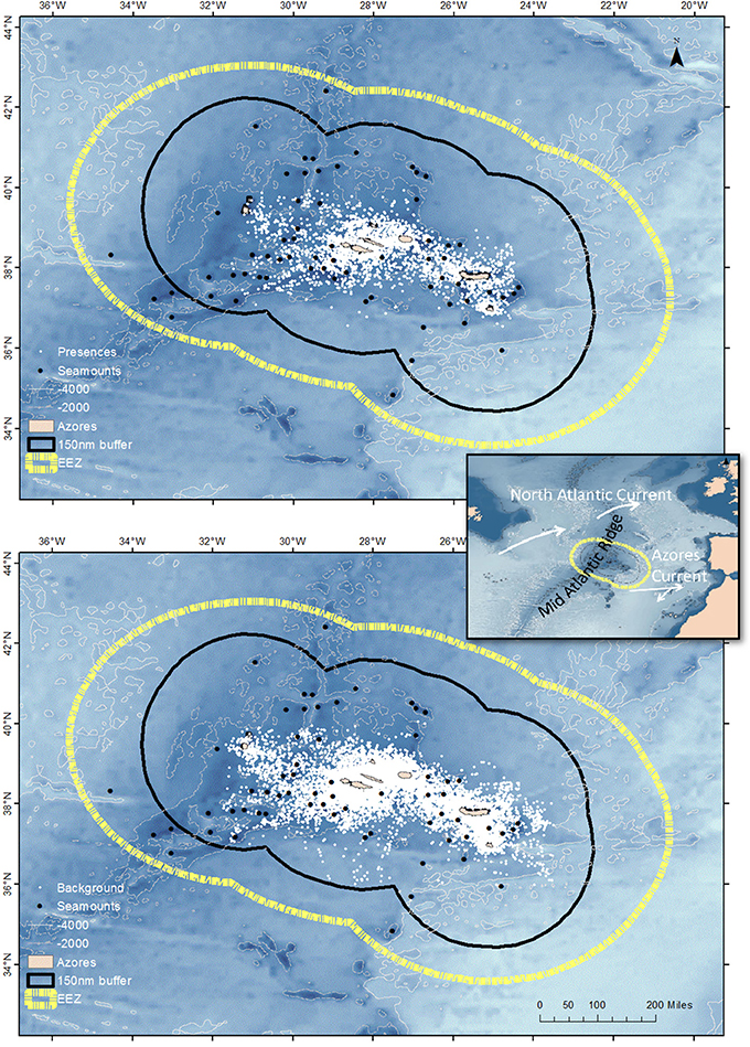
Figure 1. Cetacean sighting positions (top panel) and environmental samples (lower panel) within the study region. The position of the Azores archipelago in the North Atlantic and the main oceanographic structures mentioned in the text are show in the inset. The yellow stippled line represents the limit of the 200 nautical miles economic exclusive zone (EEZ) and the thin black line represents the limit of the 150 nautical miles buffer applied to the predictions from the MaxEnt models. Bathymetry is shown as a scale of blue; the 2000 and 4000 m isolines are also shown. Large seamounts are shown as black dots; smaller seamount-like features are not shown.

Cetacean Occurrence Data

Cetacean occurrences were obtained from the Azores Fisheries Observer Programme (POPA), from May to November, between 2004 and 2009 (Figure 1). POPA places trained observers aboard tuna-fishing vessels to monitor and collect information on the fishery and on the presence and behavior of cetaceans, seabirds and turtles. Cetacean surveying effort is conducted when the vessel is cruising or searching for fish schools. During on-effort periods, vessel position and environmental conditions are recorded every 30 min or whenever vessel course changes >20°. All sightings and vessel positions are georeferenced using global positioning system with datum São Braz (EPSG 2190). Sightings are coded according to reliability of species identification, from 0 (low confidence) to 3 (definitive). In this study we analyzed only sightings recorded during on-effort survey periods conducted in sea states on the Beaufort scale ≤3 and with an identification score of 3. Each sighting was considered as a single occurrence, irrespective of the number of individuals within the group.

To avoid bias from clustered points (Hernandez et al., 2006) we used a Geographic Information System (ArcGIS 10.1; ESRI, Inc.; hereby referred as ArcGIS) to identify multiple occurrences within individual grid cells in the environmental space defined by the predictor variables (see Section Environmental data). When more than one occurrence was found within an individual grid cell, one occurrence was chosen randomly (to avoid temporal bias) and kept in the dataset and all remaining occurrences within that grid cell were removed from the dataset. Since this spatial filtering means that only one occurrence per grid cell was used to fit the models, in practice the number of occurrences used to fit the models and presences (grid cells where a species was detected) is the same, even if the number of sightings reported for the species was higher.

Occurrence data were available for 18 cetacean species or groups of species, but models were created only for 16 taxa (15 species and 1 genus: Table 3). Only four unequivocal sightings were recorded for the humpback whale (Megaptera novaeangliae) and one for either the pigmy or dwarf sperm whales (Kogia sp.), which were considered insufficient for creating credible models (Wisz et al., 2008; Herkt et al., 2016). Sightings of beaked whales of the Genus Mesoplodon were pooled together (Mesoplodon spp.) due to their ecological similarity and difficulty in identifying these animals to the species level at sea. Models for blue (Balaenoptera musculus), fin (B. physalus), and sei (B. borealis) whales were presented elsewhere (Prieto et al., 2016), but here they are combined with models of other species to produce cetacean relative richness maps for the Azores.

Environmental Data

A set of 18 candidate environmental variables (Table 1) were selected based on their perceived ecological relevance for cetaceans (Baumgartner et al., 2001; Cañadas et al., 2002; Davis et al., 2002; Yen et al., 2004; Johnston et al., 2008; Santora et al., 2010; Baines and Reichelt, 2014; Mannocci et al., 2014, 2015). Depth was obtained from the grid-centered bedrock version of the ETOPO-1 digital elevation model (Amante and Eakins, 2009). Remotely sensed night-time sea surface temperature (NSST) was derived from standard mapped images (level 3, monthly average composite) collected by the Moderate Resolution Imaging Spectroradiometer (MODIS) instrument aboard NASA's Aqua satellite and obtained from the Ocean Color Discipline Processing System (Campbell et al., 1995). Remotely sensed near-surface primary productivity indicated by Chlorophyll-a concentration (Chl-a) data was used as a proxy for secondary production and was also derived from data collected by Aqua MODIS, with the same spatial and temporal resolutions as NSST. Location and physiography of seamounts and seamount-like features were obtained from Morato et al. (2008a) and digitized as a georeferenced database.

TABLE 1

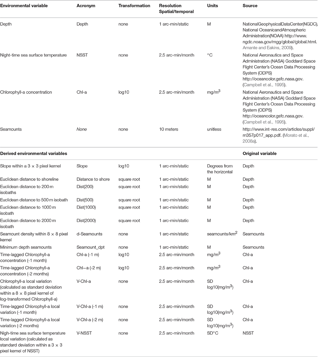
Table 1. Candidate environmental variables used in the variable selection procedure prior to model fitting (see Supplementary Material S1 for details).

The remaining variables were derived from those four using ArcGIS. Variables based on distance/area calculation were first processed in UTM zone 26N with horizontal datum WGS84, and then all variables were projected to an Equidistant Cylindrical projection with horizontal datum WGS84 and resampled to the same extent, with 2.5 arc-min resolution, using bilinear interpolation. Derived variables were: terrain slope; distance to shore, distance to bathymetric isoline (Dist_(n), with “n” representing isoline depth); seamount density (d-Seamounts); minimum depth of seamount (Seamount_dpt); time-lagged Chlorophyll-a concentration for one (Chl-a_(−1m)) and two (Chl-a_(−2m)) months prior to the sighting month; local variation of Chlorophyll-a concentration (V-Chl-a; calculated as standard deviation within a 8 × 8 pixel kernel); time-lagged local variation of Chlorophyll-a concentration for one (V-Chl-a_(−1m)) and two (V-Chl-a_(−2m)) months prior to the sighting month; and local variation of night-time sea surface temperature (V-NSST; calculated as standard deviation within a 3 × 3 pixel kernel).

Predictive Modeling

Our dataset comprised only presence records thus we chose to use the software MaxEnt 3.3.3k (Phillips et al., 2006; Dudík et al., 2007) to create monthly (April to September) SDMs for the 16 cetacean taxa in this study.

The MaxEnt algorithm was developed to infer species distributions from presence-only data as a function of a set of ecologically relevant environmental covariates (Phillips et al., 2006; Dudík et al., 2007). Models created in MaxEnt can be used to produce habitat suitability maps which translate the potential distribution of the modeled species under specific environmental conditions (Phillips et al., 2006). We have chosen to use MaxEnt partially because the algorithm has been shown to be among the best performing methods for presence-only data, yielding results comparable to presence-absence methods (Elith et al., 2006; Wisz et al., 2008; Elith and Graham, 2009; Aguirre-Gutiérrez et al., 2013; Duan et al., 2014). Additionally, we were concerned about the effect of small sample sizes from some of the species in this study. Different works quantifying the effect of sample size on the performance of multiple species distribution modeling algorithms sugest that MaxEnt is one of the most consistent accross sample sizes, even at sample sizes lower than 10 occurrences (Hernandez et al., 2006; Pearson et al., 2007; Wisz et al., 2008; Aguirre-Gutiérrez et al., 2013). However, it must be emphasized that even with MaxEnt, best performance is achieved when models are based on 30 or more occurrences and at lower sample sizes models can yield inconsistent results (Pearson et al., 2007; Wisz et al., 2008; Shcheglovitova and Anderson, 2013). Details about MaxEnt theoretical principles and utilization can be found in Phillips et al. (2006), Phillips and Dudík (2008), and Elith et al. (2011).

MaxEnt predictions are strongly affected by sample selection bias (Phillips et al., 2009); models suffering from that type of bias can be considerably improved by drawing the environmental samples from a distribution of locations with the same selection bias as the occurrence data to create an “informed” model (Phillips et al., 2009; Kramer-Schadt et al., 2013). POPA survey effort is dependent on fish distribution and fishing strategies of the boat captains and is neither random, nor homogeneously distributed (Silva et al., 2002, 2011). We dealt with sample selection bias in the POPA dataset by drawing environmental samples from a set of 10,000 randomly chosen vessel data points, thus creating informed models to correct for sampling bias (Figure 1).

MaxEnt accepts variables in two formats: (1) gridded, as raster datasets, or (2) in tabulated format, called “samples with data” (SWD) in the MaxEnt jargon (Elith et al., 2011). Raster datasets do not include a temporal dimension and thus models based on gridded datasets cannot account for seasonal changes in the variables. The only way to account for seasonality using gridded datasets is by partioning the data to produce a different model for each season, which in our case was not possible due to low sample sizes. Instead, we used SWD to enable including dynamic variables such as NSST, Chl-a, and variables derived from those. For any given sample, the values for dynamic variables were obtained for the respective month.

Cetacean occurrences and vessel data points were merged with candidate environmental variables in ArcGIS. Occurrences with missing corresponding environmental variables were discarded (Table 2).

TABLE 2

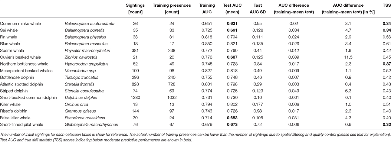
Table 2. Presences used to fit SDMs and performance statistics.

Monthly (April-September) species distribution maps were produced for all species, from the individual models fitted in MaxEnt, after model tuning (see Supplementary Material S1 for details on model tuning). Dynamic environmental variables used to create those maps (NSST and Chl-a, and derived variables) were based on monthly climatologies covering the study period (2004–2009). Maps were produced by MaxEnt using logistic habitat suitability scores varying from 0 (unsuitable habitat) to 1 (highly suitable habitat), and exported in rasterized format. The multivariate environmental similarity surface (MESS) function in MaxEnt (Elith et al., 2010) was used to test the similarity between environmental conditions found during model fitting and the prediction area. Subsequently, based on the most restrictive results from the MESS analysis (Figure S1), prediction maps for all species were limited to an area within a buffer of 150 nautical miles around the Azores islands (Figure S1). Additionally, we enabled the “fade by clamping” option in MaxEnt to prevent extrapolations outside the environmental range of the training data (Owens et al., 2013). MaxEnt was run in command line mode using scripts, with maximum number of iterations set to 5000 for all models to guarantee model convergence.

The performance of models was assessed using two metrics: (1) the area under the receiver operating characteristic curve metric (AUC), which is threshold-independent (Fielding and Bell, 1997), and (2) the true skill statistic (TSS), which is threshold-dependent (Allouche et al., 2006). Calculations were performed using MaxEnt model outputs and in-built functionalities in biomod2 package for R (Thuiller et al., 2009).

We created test-SDMs for each species by splitting presences into training (90% of occurrences) and test (10% of occurrences) datasets using a 10-fold cross-validation procedure to estimate predictive performance on held-out folds (Elith et al., 2011; Peterson et al., 2011).

The AUC is widely used to assess predictive power of distribution models. In methods using presence-absence data, the AUC expresses the ability of the model to discriminate between suitable and unsuitable habitat (Fielding and Bell, 1997; Wiley et al., 2003). In presence-only methods, however, AUC is interpreted as being a measure of the ability of the model to discriminate between known presences and environmental samples (Phillips et al., 2006).

In presence-absence methods an AUC = 1.0 translates a perfect performance and AUC = 0.5 a performance no better than random (Fielding and Bell, 1997). However, Wiley et al. (2003) have shown that for presence-only methods the maximum achievable AUC is area dependent, being a quantity 1−a/2 (where “a” is the fraction of the geographical area covered by the species' unknown true distribution); consequently, in that case, AUC always assumes a value <1 (Wiley et al., 2003; Phillips et al., 2006). A wide range of values is used by different sources to categorize the predictive power of models based on AUC values (Merckx et al., 2011). Here we assumed that models with mean test-AUC values of AUC < 0.7 had poor predictive performance, 0.7 ≤ AUC < 0.8 moderate, and AUC ≥ 0.8 good to excellent performance (Merckx et al., 2011; Peterson et al., 2011; Duan et al., 2014).

Additionally, we investigated model robustness by computing the test-AUC standard deviation (SD) and the difference between the train-AUC values of each species' final SDM (SDM_f; using all presences) and the mean test-AUC values of the SDMs (Table 2). Low test-AUC SD and/or small difference between the train-AUC and mean test-AUC values indicate model robustness (Herkt et al., 2016).

Currently there is an open discussion about the reliability of AUC to measure the performance of models based on presence-only methods, and several authors advocate combining different model performance criteria to have a more robust evaluation of the results (Lobo et al., 2008; Merow et al., 2013; Radosavljevic and Anderson, 2014). To have a complementary measure of model performance we calculated the true skill statistic (TSS), which is similar to the well-known Kappa statistic (Fielding and Bell, 1997; Allouche et al., 2006). Similarly to the Kappa statistic, TSS reflects the rate of false positive and negative predictions, but has the advantage of not being sensitive to the frequency of presence points (Allouche et al., 2006). Allouche et al. (2006) defined TSS as:

$\begin{array}{l}\mathrm{\text{TSS}}=\mathrm{\text{sensitivity}}+\mathrm{\text{specifity}}-1\end{array}$

with sensitivity translating the proportion of observed presences that are correctly predicted as presences, and specificity as the proportion of observed absences that are correctly predicted as absences. Similarly to Kappa, the TSS can assume values between −1 and 1 and values of TSS < 0.2 can be considered as reflecting poor model predictive performance, 0.2 ≤ TSS < 0.4 as fair, 0.4 ≤ TSS < 0.6 moderate, and TSS ≥ 0.6 as good to excellent performance (Landis and Koch, 1977). As TSS is threshold-dependent, the suitability scores returned by MaxEnt must be converted in binary values using a threshold for predicting presence, which was done internally in biomod2 by testing a range of possible threshold values and selecting the value that maximized TSS.

Species Richness Maps

As we were also interested in identifying areas and seasons with conditions for increased cetacean biodiversity, we produced monthly (April–September) cetacean species richness maps. These maps were created by combining (stacking) the individual species prediction maps created in MaxEnt, to produce stacked species distribution models (S-SDMs) for each month evaluated in this study.

Usually, S-SDMs are built by creating binary (present or absent) distribution maps for each species and then calculating the number of predicted species present in a given site (Ferrier and Guisan, 2006). It is clear that the selection of the threshold to transform the continuous outputs from individual SDMs into binary values can heavily influence the predictive performance of the resulting S-SDMs. Thus, this approach must be only used when there is good ecological information to support the choice of the threshold value (Benito et al., 2013). Additionally, since S-SDMs do not account for negative biotic interactions (such as competition and inhibition), the practice of summing binary SDMs tends to lead to overprediction of species richness (Algar et al., 2009; Dubuis et al., 2011). Calabrese et al. (2014) and D'Amen et al. (2015) present convincing evidence that simply summing the per-site predictions of occurrence probabilities from individual SDMs is preferable to the widespread practice of setting arbitrary thresholds to obtain binary predictions and then combining those into a S-SDM.

Here we used the software ENM Tools (Warren et al., 2010) to standardize habitat suitability scores from each species prediction maps so that all scores within the geographic space summed to 1, making predictions comparable among SDMs. The resulting processed maps were then combined in ArcGIS by summing the standardized raw scores from equivalent cells to create the final monthly species relative richness maps. These maps do not intend to give an estimate of how many species are present in a given site, but only where cetacean richness is expected to be higher when compared to adjacent areas.

Results

After quality control and spatial filtering, 84.5% of the sightings (2878) were retained (Table 2; Figure 1). Of these, nearly 73% belonged to three species: sperm whale (11.7%); Atlantic spotted dolphin (25.3%); and short-beaked common dolphin (35.9%). Of the 16 SDMs, 14 were based on 20 occurrences or more, and the remaining on more than 10 occurrences (Table 2).

The majority of the SDMs presented moderate to good discrimination power, with test-AUC scores ≥0.7 (n = 11), and TSS scores ≥0.4 (n = 12) (Table 2). Overall, there was good agreement among the two metrics: models with low test-AUC scores tended to also have low TSS values (although always well above 0.2), moderate test-AUC corresponded to moderate TSS values and the highest test-AUC scores tended to correspond to high TSS scores (Table 2). However, based on the TSS scores, only one model (for the blue whale) was considered as having above than moderate performance, compared to three models based on the test-AUC scores (Table 2).

The difference between mean AUC values from test-SDMs and the corresponding training AUC from the SDM_f was low (mean: 2.9%; median: 2.3%; Table 2) and most models had low test-AUC SD, comparable with similar multi-species studies (e.g., Herkt et al., 2016), indicating overall model robustness.

From the 18 variables initially considered, only half had a permutation importance score >5 and were considered as having a meaningful role in defining the environmental niche for the species (please refer to Supplementary Material S1 for definition of permutation importance and its use in variable selection). No single variable was retained in all models. The variable most commonly retained in the models was distance to shore (retained in 12 models), followed by the time-lagged Chlorophyll-a local variation 2 months prior to the sighting month (9 models), and Chlorophyll-a concentration from the previous month to the sighting date and nighttime sea surface temperature (8 models each). The remaining variables were retained in 2–6 models (Table 3).

TABLE 3

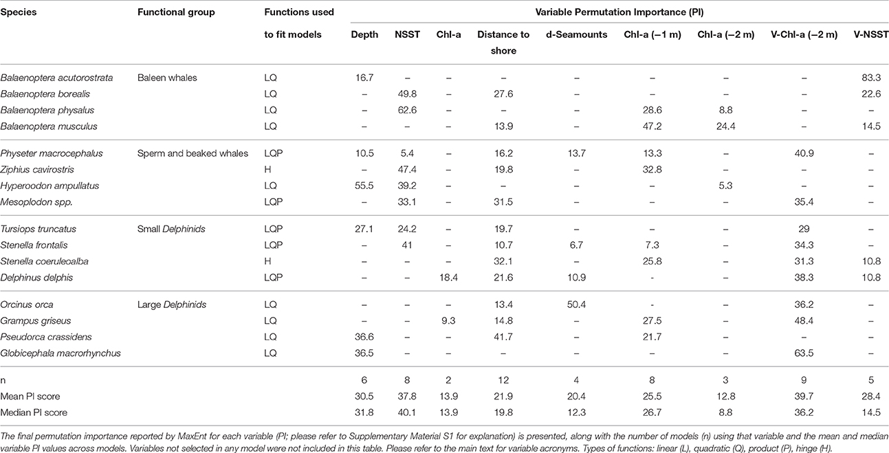
Table 3. Functions and environmental variables used to build final SDMs, after model tuning, by species.

Discussion

Interpretation of Models

Giving full treatment of each species here is unpractical and beyond the scope of this work. Instead we summarize the main findings for four functional species groups according to phylogeny and ecology: (1) baleen whales (genus Balaneoptera); (2) sperm and beaked whales (genera Physeter, Mesoplodon, Hyperoodon, and Ziphius); (3) small Delphinids (genera Delphinus, Stenella, and Tursiops); and (4) large Delphinids (genera Globicephala, Grampus, Orcinus, and Pseudorca). Where relevant we highlight important results of individual taxa.

As an illustrative example, we present the model projections of potential species distribution for the Atlantic spotted dolphin in Figure 2. All 96 monthly (April-September) maps of potential species distribution based on the MaxEnt final SDMs, as well as the 34 maps for species richness are freely available online as raster grid files from the Pangaea database: https://doi.org/10.1594/PANGAEA.864511.

FIGURE 2

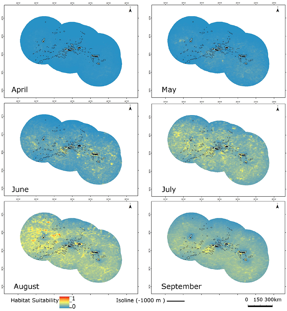
Figure 2. Monthly potential distribution (April-September) of the Atlantic spotted dolphin (Stenella frontalis), from MaxEnt modeled habitat suitability. Warmer colors correspond to increased habitat suitability. The 1000 m isoline is indicated by the thin black lines.

Baleen Whales

The spatio-temporal patterns of the four species in this group were quite variable, probably due to different dietary preferences, energetic requirements, and species migratory behaviors. Potential distribution for the minke whale (Balaenoptera acutorostrata) was essentially homogenous throughout the region and the period analyzed. The model for that species was chiefly driven by local variation in the night-time sea surface temperature and, at a much lower extent, by depth (Table 3). These results are in line with results reported by Silva et al. (2014) who did not find any apparent seasonal pattern for the species from stranding records. However, the model had the lowest AUC scores of all models and also one of the lowest TSS scores, and should be interpreted with reserve. Blue (B. musculus) and fin (B. physalus) whales' potential habitat differed seasonally with a strong latitudinal component, driven in great part by temporal variation in the primary productivity in the region, but also water temperature in the case of the fin whale. In contrast to the blue and fin whale models, the sei whale (B. borealis) model did not retain variables related to primary production (Table 3). In combination these results agree with previous work suggesting that the region may play different ecological roles for migrating baleen whales, being a foraging area for blue and fin whales but only a transit area for sei whales (Silva et al., 2013; Prieto et al., 2014). A more in-depth interpretation of the models for the blue, fin and sei whale is given in Prieto et al. (2016).

Sperm and Beaked Whales

Sperm (Physeter macrocephalus) and beaked whales are all deep diving cetaceans and are often considered to be essentially teutophagous (Mead, 2002). However, recent research has shown that beaked whales may show dietary plasticity (MacLeod et al., 2003). In the Azores, the diet of Sowerby's beaked whale (Mesoplodon bidens) is composed essentially of meso- and bathy-pelagic fish, with little contribution from cephalopods (Pereira et al., 2011). Night-time sea surface temperature was retained in the models of all species in this group and, apart from the sperm whale, was highly influential in the models consistent with a seasonal presence of beaked whales in the region (Table 3). From combined survey and stranding data Silva et al. (2014) report an almost year-round presence of Mesoplodon and Cuvier's (Ziphius cavirostris) beaked whales, with a peak in summer months. The same authors recorded the presence of the northern bottlenose whale (Hyperoodon ampullatus) only during the summer months. These results are in agreement with our results that show improving habitat conditions for all beaked whales with progression of the summer months. Beaked whales can be considered cryptic, as sightings of this group are heavily affected by sea conditions (e.g., Waring et al., 2008). The apparent improvement of habitat suitability with progression of the season predicted by the models can be an artifact of higher detectability during summer months. The model for the Cuvier's beaked whale had the largest drop in AUC mean value of test-SDM when compared with the AUC of the SDM_f (11.5%). Thus, predictions based on this model should be interpreted with some reserve.

The sperm whale model had the highest number of variables retained among all models (Table 3), indicating that their environmental niche in the region is dependent on the combination of several conditions, possibly related to different life-history requirements. The variable that contributed most to the sperm whale model was the time-lagged Chlorophyll-a local variation (2 months prior to sighting month), which may be an indication that they associate with oceanographic structures that enhance biological productivity. Chlorophyll concentration of the prior month to the sighting month was also included in the model. Other studies have found primary productivity to be a good predictor of sperm whale distribution, despite being a distal predictor due to large spatial and temporal lags between the onset of primary productivity and cephalopod presence (Jaquet, 1996; Jaquet and Gendron, 2002; Praca et al., 2009). Morato et al. (2008b) report that sperm whale sighting frequencies in the Azores were not influenced by distance to seamounts. In contrast, Waring et al. (2008) report that sightings of sperm whales made along the mid-Atlantic ridge in the summer of 2004, were usually made at the tops of seamounts and rises. This apparent contradiction may be due to the effect of differing feeding ecologies of male and female sperm whales. Most of the sperm whale sightings reported by Waring et al. (2008) were made north of 50° North, where only male sperm whales are supposed to occur (Whitehead, 2009). While female sperm whales feed mostly on cephalopods, males have a more catholic diet that may include large demersal fish (Whitehead, 2009). Our results are in agreement with those reported by Morato et al. (2008b), seamount presence was not retained in the sperm whale model (or in any other model for that matter). However, seamount density was retained in the model, with a reasonably high permutation importance (13.7; Table 3). In fact, the potential distribution maps for the sperm whale highlight some seamount complexes as preferential habitat, especially during spring and early summer months. One possible explanation for the retention of this variable in this and other models is that seamount density reflects increased topographic complexity that may be important at creating physical processes that aggregate enough productivity to attract visitors (Morato et al., 2015).

Small Delphinids

All models for the small dolphins retained distance to shore and time-lagged Chlorophyll-a local variation (Table 3). Our results highlight a succession pattern in the seasonality of the common (D. delphis) and spotted (Stenella frontalis) dolphins that had already been detected by Silva et al. (2014). Both species present a marked seasonality, but while the potential distribution of the common dolphin compresses with the progression of the summer, the potential distribution of the spotted dolphin expands. Silva et al. (2014) suggested that the phenomenon could be related with the effect of the warming water on prey distribution, or to strategies for reducing interspecific competition for prey. The retention of SST and Chl-a derived variables in both models does not allow to identify which of these mechanisms may be at play. As the season progresses the potential distribution of the common dolphin becomes restricted to some seamount complexes, indicating that seamounts may play an important role in maintaining conditions for the occurrence of the species in the region throughout the year. Morato et al. (2008b) report that the common dolphin was significantly more abundant in the vicinity of shallow seamounts, supporting our results.

The model for the striped (S. coeruleoalba) shows a strong variation of the potential habitat with season. Silva et al. (2014) report an almost continuous presence of the striped dolphin in the Azores, with higher encounter rates between May and July. Our results indicate that the distribution of the striped dolphin is strongly influenced by water temperature, as night-time sea surface temperature was the most important variable in that model (Table 3). This result might explain the higher encounter rates in early to mid-summer detected by Silva et al. (2014).

The bottlenose dolphin (Tursiops truncatus) model also indicates an effect of the season on the distribution of the species. As expected from the presence of resident animals near the islands (Silva et al., 2008), physiographic variables (distance to shore and depth) were influential in the bottlenose dolphin model, along with variables indicative of productivity distribution (Table 3). However, our model shows an expansion of the potential habitat to offshore areas up to August, and then a contraction in September.

Silva et al. (2008) report a complex pattern of residency for the bottlenose dolphin in the Azores, including residents, transients and temporary migrants. Despite a continuous presence in the region, Silva et al. (2014) reported that encounter rates with the bottlenose dolphin “varied greatly between months,” and suggested that fluctuations in encounter rates might be caused by the temporary immigration of non-resident [transient] dolphins. According to Silva et al. (2008), resident bottlenose dolphins have small, near-shore, home-ranges in disagreement with the expansion of the potential habitat predicted by the model. However, large-scale movements among islands and to offshore banks were recorded for non-resident bottlenose dolphins (Silva et al., 2008). The study by Silva et al. (2008) could not test for an effect of season on the occurrence of large-scale movements but the authors hypothesized that these movements were a response to the low density and patchy distribution of prey. Seasonal immigration of transient bottlenose dolphins combined with wider ranging behavior by non-resident dolphins during part of the year could explain the fluctuations in the extent of potential habitat predicted by our model for the species.

Large Delphinids

The predictions for the four species in this group varied substantially. Based on their feeding ecology, the Risso's dolphin (Grampus griseus) and the short-finned pilot whale (Globicephala macrorhynchus) can be considered more similar to each-other, as they are both deep divers and prey preferentially on cephalopods (Baird, 2009a; Olson, 2009). On the other hand, the killer whale (Orcinus orca) and the false killer whale (Pseudorca crassidens) are both top predators with generalist diets that can include cephalopods, large fish and also marine turtles and other marine mammals (Baird, 2009b; Ford, 2009). The Risso's dolphin model indicates an expansion of the potential distribution up to June and then a contraction after that month. Coastal habitats, however, seem to be important during most of the period, which may be related to the presence of resident groups using these areas as foraging, calving and nursing habitats (Hartman et al., 2014, 2015). In contrast, the short-finned pilot whale model indicates a potential distribution that is spatially and temporally homogeneous. However, the short-finned pilot whale model had poor performance, based both on the AUC and TSS scores, and should be interpreted with reserve. Additionally, and despite our data quality control, it cannot be ruled out that some sightings attributed to this species are in fact of its sister species (Globicephala melas), that sometimes is seen in the region and is almost indistinguishable from the short-finned pilot whale at sea (Prieto and Fernandes, 2007). The killer whale model was chiefly influenced by seamount density and, to a much smaller extent distance to shore, with no temporal pattern being detectable. Based on combined sighting and strandings data, Silva et al. (2014) also failed to detect any temporal trend for this species. Finally, the false killer whale model shows a potential distribution highly influenced by the mid-Atlantic ridge and seamounts or seamount-like structures.

Cetacean Richness

When all species are considered together, the distribution of areas with increased relative species richness is somewhat diffuse, showing great spatial and temporal variation (Figure 3). This is not surprising taking into consideration the wide differences in trophic ecology and natural history among the 16 taxa and the fact that most species in this study have predominantly pelagic habits. Not surprisingly, since it was based in the same dataset, the encounter rates maps in Silva et al. (2014) also show a great heterogeneity in the distribution patterns of cetaceans in the region. However, our models show seasonal effects that could not be detected with the methodology utilized by Silva et al. (2014).

FIGURE 3

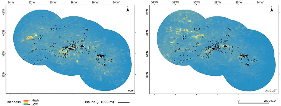
Figure 3. Combined predicted cetacean richness in spring (May) and summer (August). Color shading indicates relative species richness, with warmer colors corresponding to increased richness.

Pelagic habitats are a function of complex oceanographic processes that can be highly dynamic in space and time (Hazen et al., 2013; Scales et al., 2014). Pelagic features can be classified in three categories according to their predictability: static bathymetric, persistent hydrographic and ephemeral hydrographic features (Hyrenbach et al., 2000). Most marine top predators are known to track productivity associated with meso- and sub-mesoscale oceanographic structures (fronts, eddies, and filaments) that are often transient in nature (Tew Kai et al., 2009; Scales et al., 2014). However, static seabed features may influence and even originate persistent hydrographic features, which can lead to the creation of predator hotspots (Bouchet et al., 2015). That effect is apparent from our predictions, more notably for small and large dolphins, over the seamount complex located southwest of the central group of islands in the Azores, identifiable by the 1000 m isoline (Figures 5, 6).

The richness maps organized by functional groups (Figures 4–7) offer a more focused perspective, helping to better interpret the results.

FIGURE 4

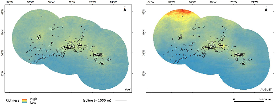
Figure 4. Combined predicted richness of baleen whales in spring (May) and summer (August). Color scheme as in Figure 3.

The relative species richness maps from all baleen whale models combined are marked by the strong latitudinal component from the individual blue and fin whale models. The combined predictions do not show any evident affinity of baleen whales as a group to specific oceanographic or topographic but the latitudinal progression of conditions is clearly seen when comparing predictions for spring and summer months (Figure 4).

The maps of relative species richness for small and large Delphinids show the likely influence of transient oceanographic structures, translated by temporary sites of increased richness with filamentous or circular configuration. However, for both groups the species richness is increased also in coastal zones of some of the islands and, as mentioned earlier, around and over seamount complexes, as in the case of the seamounts just southwest of the central group of islands, but also around other seamount and seamount-like structures (Figures 5, 6).

FIGURE 5

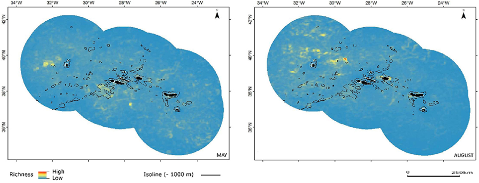
Figure 5. Combined predicted richness of small dolphins in spring (May) and summer (August). Color scheme as in Figure 3.

FIGURE 6

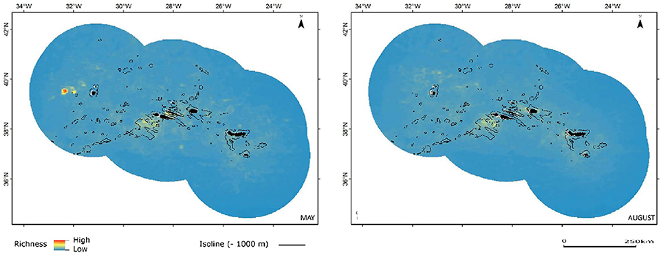
Figure 6. Combined predicted richness of large dolphins in spring (May) and summer (August). Color scheme as in Figure 3.

Combined sperm and beaked whale richness seems to be also increased by transient oceanographic features, seen as temporary sites of increased richness with filamentous or circular configuration (Figure 7). There seems to be an apparent, although difficult to discern, effect of seamount complexes in increasing richness for this group (Figure 7). However, and unlike the results for most of the dolphins, the sperm and beaked whales models show lowest habitat suitability in the shallowest areas over seamounts and seamount-like structures, as well as coastal areas. Instead, the richness appears to increase in deeper waters, which is in agreement with the deep diving habits of the taxa in this group (Figure 7).

FIGURE 7

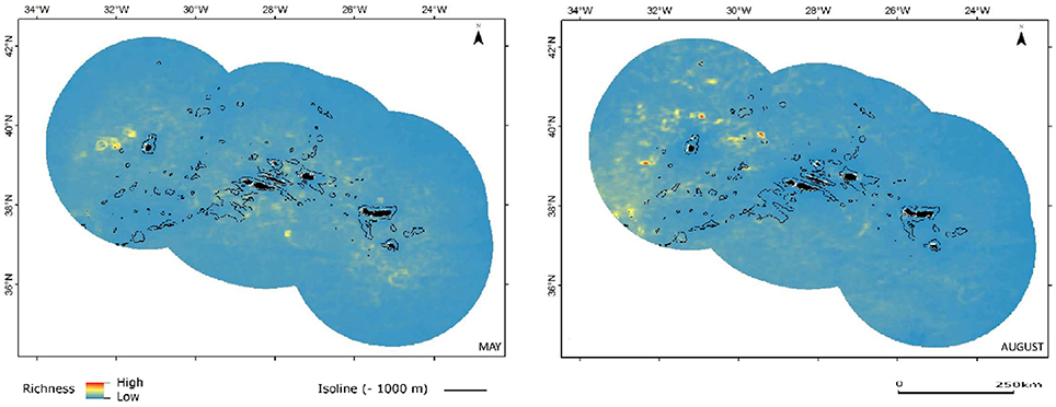
Figure 7. Combined predicted richness of sperm and beaked whales in spring (May) and summer (August). Color scheme as in Figure 3.

Overall, the relative species richness maps highlight the fact that cetaceans utilize large areas and actively seek dynamic oceanographic features believed to be associated with increased biological productivity, making the identification of delimited priority areas a complex task. However, our results do show areas that hold increased species richness, such as some seamount complexes and coastal areas around islands, deserving special treatment regarding management of human activities that may threaten cetaceans.

Performance and Caveats of Models

By choosing a modeling technique specifically designed to handle presence-only data (MaxEnt), carefully implementing a data quality control and tuning models for each species individually, we were able to build plausible habitat suitability models, using existing sighting data collected with a consistent methodology by an observer fisheries program (POPA).

Model evaluation metrics indicate that, overall, models had reasonable performance, and are useful both for ecological studies and to support decision making. The majority of the models showed moderate discrimination power (based on test-AUC values and the true skill statistic) and appropriate robustness (based on prevailing low SD in test-AUC values and small differences between AUC from the SDM_f and test-AUC). However, there is ample space for improvement in future revisions of these models.

Data quality control dictated that some models had to be fitted with low number of occurrences (<20). Although MaxEnt has been repeatedly shown to perform well at small sample sizes, models using few occurrences can yield inconsistent results (Wisz et al., 2008; Aguirre-Gutiérrez et al., 2013). Additionally, we could only carry out internal evaluations of performance as no independent dataset was available. Ideally spatially independent data should be used for evaluating model performance, since performance metrics are inflated by the effect of spatial autocorrelation between training and test data (Bahn and McGill, 2013). It is likely that the performance metrics we used are positively biased, by the combined effects of small sample size and the lack of an independent test dataset (Randin et al., 2006; Bean et al., 2012). We intend to address those issues in future revisions of the models.

An important, although subjective, part of model evaluation is visually examining fitted functions and mapped projections to detect unexpected model responses or predictions (Elith et al., 2010). As mentioned above, we carefully inspected fitted functions plots (partial dependence plots; Supplementary Material S2) as part of the tuning process (detailed in Supplementary Material S1) and evaluated the ecological coherence of the function plots for each variable and species. Despite some minor artifacts, the mapped projections did not produce any unrealistic patterns, improving our confidence on the models. Nevertheless, when creating the models we had to make some assumptions that may have affected the estimation of the relationships with environmental covariates, at least for some species. Due to small sample sizes, we could not subset the data to create seasonal models; instead we created a single model for each species and then projected that model onto the environmental conditions of different months. In doing so, we assumed that the habitat preferences of the species do not drastically change with time. If that assumption is not met the relationships estimated by the models may be biased. Granted more sightings are available, this issue can be investigated and addressed in the future by creating models for distinct seasons.

There may also be an effect of using climatologies to project the models that could potentially affect predictions. Since the data from dynamic variables used to fit the models were quasi-contemporaneous (same month) to the sightings, these data will present more variability than the climatologies used to project the models (which will smooth out interannual variability). In extreme cases that effect could be an issue because the predicted habitat suitability will tend to be underestimated (or overestimated). For example, if a variable was low for most of the years and high in 1 year, and if the species was present only in that particular year, the model would fit a relationship to that variable and depending on the modeled relationship the predictions could be unreasonable. The predictions could indicate that the habitat suitability for the species in the region is low (due to the smoothing effect of the climatologies), when in fact it would be high during years with more extreme conditions. This issue would be more concerning for species for which the Azores are positioned in the limits of their geographical range, such as the Bryde's whale (Balaenoptera edeni), the Fraser's dolphin (Lagenodelphis hosei) and the rough toothed dolphin (Steno bredanensis), all tropical species that are rare visitors to the region (Silva et al., 2014). However, we did not include species considered as rare visitors to the region in this work. We find highly unlikely that our models were fit to extreme values, because all species for which models were fit were present in multiple years.

To the best of our ability, we tried to follow the principle of using explanatory covariates that are reasonably proximal to the target species (Austin, 2002). For example, we included water temperature (NSST) as a covariate in our models because cetacean distribution is highly influenced by thermal preferences (MacLeod, 2009; Lambert E. et al., 2014). Additionally we implemented a methodology for eliminating variables with marginal predictive importance, in order to obtain the most parsimonious SDMs possible. However, we were limited by the currently available variables. Prey abundance and quality directly influence cetacean distribution, and as such should ideally be included in SDMs as proximal predictors (Guisan and Zimmermann, 2000; Young et al., 2015). However, that information was not available and it can take years before it will be. Instead, we used Chlorophyll-a (Chl-a) and the derived variables as proxies for prey distribution. These variables may have limited explanatory power due to potential large lags between oceanographic processes and biological response of cetacean prey, especially in the case of upper trophic level cetaceans (Lambert C. et al., 2014). In the future we intend to integrate prey data by fitting a 3-dimentional model for mid-trophic organisms to the Azores pelagic ecosystem conditions and then nesting it into our own SDMs (Lehodey et al., 2010; Lambert C. et al., 2014).

We also intend to include a wider range of dynamic covariates, once they are available, in order to identify areas of predictable or persistent oceanographic activity that are potentially important for cetaceans and that were not detected with our original set of covariates. For example, the inclusion of fine-scale information on circulation patterns derived from models tunned at the regional scale (e.g., Sala et al., 2015) could help interpreting some of the spatial patterns and variability shown by the models.

Conclusions

High-resolution species distribution data for marine taxa are still scarce but essential in ecosystem functioning research and to implement ecosystem-based management through marine spatial planning (MSP) (Beck et al., 2012; Shucksmith et al., 2014). Here we present the first SDMs for 16 cetacean taxa at the scale of the entire Azores archipelago up to 150 nautical miles from shore, at a fine spatial resolution. We also produced cetacean relative richness maps that may both inform MSP efforts by highlighting discrete important areas for cetaceans and help identify potential local processes influencing large-scale macroecological patterns (Belmaker and Jetz, 2011).

Species distribution models are valuable in identifying areas that can be effective in protecting marine predators (Pérez-Jorge et al., 2015; Young et al., 2015). Our models show areas (namely near or over seamounts) that appear to hold favorable conditions to the occurrence of some of the species investigated in this study, especially among dolphins. These areas should deserve special attention when considering MSP actions. Nevertheless, our results also highlight the fact that cetacean distribution can vary widely at relatively short periods of time as they track dynamic oceanographic structures. Any effort at protecting cetaceans and their habitats must take the temporal dimension into account. Dynamic ocean management (DOM) is a relatively recent concept that aims to refine the temporal and spatial scales of managed areas by integrating near-real time biological, oceanographic and socio-economic data (Maxwell et al., 2015). We acknowledge that DOM still faces several challenges for widespread application as it has only been tested on a few systems and for few species, and requires a large amount of resources (Maxwell et al., 2015; Mills et al., 2015). However, we argue that we must take steps in the direction of integrating DOM with more traditional MSP approaches if we are to effectively protect pelagic species with very dynamic distributions, especially in face of predicted effects of climate change (Fulton et al., 2015).

Our models provide a new baseline regarding the spatial and temporal distribution patterns of cetaceans in a vast area of the Azores marine ecosystem. However, they lack some essential information about species density and abundance. In the future, efforts should also be made to regularly collect data under conditions that enable the application of more sophisticated modeling techniques such as density surface modeling (DSM) and multi-species DSM (Kissling et al., 2012). Data for other seasons are also lacking and efforts should be made to fill that gap.

At the core of the SDMs presented here are the data collected by POPA. Despite not being designed as a cetacean monitoring program, POPA has two great advantages: it is a long-term dataset and follows a consistent methodology. As this work has shown, using data collected from fisheries observer programs such as POPA can be a cost-efficient way of developing robust SDMs. In the future, we also plan to explore the possibility of applying novel field and statistical methods to enable using POPA sighting data to provide reliable estimates of cetacean abundance and density (Williams et al., 2006; Paxton et al., 2011; Isojunno et al., 2012).

Author Contributions

Conceived and designed the experiments: MAS, MT, RP. Performed the experiments: MT, RP. Analyzed the data: MT, RP, MAS Contributed with data: MM. Wrote the paper: MT, RP, MAS, MM.

Conflict of Interest Statement

The authors declare that the research was conducted in the absence of any commercial or financial relationships that could be construed as a potential conflict of interest.

Acknowledgments

We thank the Azores Fisheries Observer Program (POPA), which is funded by the Azorean Regional Government, and acknowledge the collaboration of all the observers, captains, and crew members of tuna vessels. We are grateful to InSeabra, Irma Cascão, and Ricardo Medeiros for assistance with the POPA dataset and with the Geographic Information System. This work was supported by FEDER funds, through the Competitiveness Factors Operational Programme - COMPETE, by national funds, through FCT - Foundation for Science and Technology, under project TRACE (PTDC/ MAR/74071/2006), and by regional funds, through DRCT/SRCTE, under projects MAPCET (M2.1.2/F/012/2011) and 2020 (M2.1.2/I/026/2011). We acknowledge funds provided by FCT to MARE, through the strategic project UID/MAR/04292/2013. RP is supported by an FCT postdoctoral grant (SFRH/BPD/108007/2015); MAS is supported by Program Investigator FCT (IF/00943/2013) and MT was supported by a research fellowship under the Exploratory project (IF/00943/2013/CP1199/CT0001) that also paid the fees for this open-access publication. IF/00943/2013 and IF/00943/2013/CP1199/CT0001 are funded by FSE and MCTES, through POPH and QREN.

Supplementary Material

The Supplementary Material for this article can be found online at: https://www.frontiersin.org/article/10.3389/fmars.2016.00202

References

Abecasis, R. C., Afonso, P., Colaço, A., Longnecker, N., Clifton, J., Schmidt, L., et al. (2015). Marine conservation in the Azores: evaluating marine protected area development in a remote island context. Front. Marine Sci. 2:104. doi: 10.3389/fmars.2015.00104

CrossRef Full Text | Google Scholar

Aguirre-Gutiérrez, J., Carvalheiro, L. G., Polce, C., van Loon, E. E., Raes, N., Reemer, M., et al. (2013). Fit-for-Purpose: species distribution model performance depends on evaluation criteria – Dutch hoverflies as a case study. PLoS ONE 8:e63708. doi: 10.1371/journal.pone.0063708

PubMed Abstract | CrossRef Full Text | Google Scholar

Algar, A. C., Kharouba, H. M., Young, E. R., and Kerr, J. T. (2009). Predicting the future of species diversity: macroecological theory, climate change, and direct tests of alternative forecasting methods. Ecography 32, 22–33. doi: 10.1111/j.1600-0587.2009.05832.x

CrossRef Full Text | Google Scholar

Allouche, O., Tsoar, A., and Kadmon, R. (2006). Assessing the accuracy of species distribution models: prevalence, kappa and the true skill statistic (TSS). J. Appl. Ecol. 43, 1223–1232. doi: 10.1111/j.1365-2664.2006.01214.x

CrossRef Full Text | Google Scholar

Amante, C., and Eakins, B. W. (2009). ETOPO1 1 Arc-Minute Global Relief Model: Procedures, Data Sources and Analysis. NOAA Technical Memorandum NESDIS NGDC-24. National Geophysical Data Center, NOAA, 19. doi: 10.7289/V5C8276M. Available online at: https://www.ngdc.noaa.gov/mgg/global/relief/ETOPO1/docs/ETOPO1.pdf

CrossRef Full Text

Austin, M. P. (2002). Spatial prediction of species distribution: an interface between ecological theory and statistical modelling. Ecol. Model. 157, 101–118. doi: 10.1016/S0304-3800(02)00205-3

CrossRef Full Text | Google Scholar

Bahn, V., and McGill, B. J. (2013). Testing the predictive performance of distribution models. OIKOS 122, 321–331. doi: 10.1111/j.1600-0706.2012.00299.x

CrossRef Full Text | Google Scholar

Baines, M., and Reichelt, M. (2014). Upwellings, canyons and whales: an important winter habitat for balaenopterid whales off Mauritania, northwest Africa. J. Cetacean Res. Manag. 14, 57–67.

Baird, R. W. (2009a). “Risso's Dolphin Grampus griseus,” in Encyclopedia of Marine Mammals, 2nd Edn., eds W. F. Perrin, B. Würsig, and J. G. M. Thewissen (New York, NY: Academic Press), 975–976.

Baird, R. W. (2009b). “False Killer Whale Pseudorca crassidens,” in Encyclopedia of Marine Mammals, 2nd Edn., eds W. F. Perrin, B. Würsig, and J. G. M. Thewissen (New York, NY: Academic Press), 405–406.

Google Scholar

Baumgartner, M. F., Mullin, K. D., May, L. N., and Leming, T. D. (2001). Cetacean habitats in the northern Gulf of Mexico. Fish. Bull. 99, 219–239.

Google Scholar

Bean, W. T., Stafford, R., and Brashares, J. S. (2012). The effects of small sample size and sample bias on threshold selection and accuracy assessment of species distribution models. Ecography 35, 250–258. doi: 10.1111/j.1600-0587.2011.06545.x

CrossRef Full Text | Google Scholar

Beaugrand, G. (2009). Decadal changes in climate and ecosystems in the North Atlantic Ocean and adjacent seas. Deep Sea Res II Top. Stud. Oceanogr. 56, 656–673. doi: 10.1016/j.dsr2.2008.12.022

CrossRef Full Text | Google Scholar

Beck, J., Ballesteros-Mejia, L., Buchmann, C. M., Dengler, J., Fritz, S. A., Gruber, B., et al. (2012). What's on the horizon for macroecology? Ecography 35, 673–683. doi: 10.1111/j.1600-0587.2012.07364.x

CrossRef Full Text | Google Scholar

Belmaker, J., and Jetz, W. (2011). Cross-scale variation in species richness–environment associations. Global Ecol. Biogeogr. 20, 464–474. doi: 10.1111/j.1466-8238.2010.00615.x

CrossRef Full Text | Google Scholar

Benito, B. M., Cayuela, L., and Albuquerque, F. S. (2013). The impact of modelling choices in the predictive performance of richness maps derived from species-distribution models: guidelines to build better diversity models. Methods Ecol. Evol. 4, 327–335. doi: 10.1111/2041-210x.12022

CrossRef Full Text | Google Scholar

Bester, M. N. (2014). “Marine mammals – natural and anthropogenic influences,” in Global Environmental Change, ed B. Freedman (Dordrecht: Springer), 167–174.

PubMed Abstract | CrossRef Full Text

Bouchet, P. J., Meeuwig, J. J., Salgado Kent, C. P., Letessier, T. B., and Jenner, C. K. (2015). Topographic determinants of mobile vertebrate predator hotspots: current knowledge and future directions. Biol. Rev. 90, 699–728. doi: 10.1111/brv.12130

PubMed Abstract | CrossRef Full Text | Google Scholar

Bowen, W. D. (1997). Role of marine mammals in aquatic ecosystems. Mar. Ecol. Prog. Ser. 158, 267–274. doi: 10.3354/meps158267

CrossRef Full Text | Google Scholar

Calabrese, J. M., Certain, G., Kraan, C., and Dormann, C. F. (2014). Stacking species distribution models and adjusting bias by linking them to macroecological models. Global Ecol. Biogeogr. 23, 99–112. doi: 10.1111/geb.12102

CrossRef Full Text | Google Scholar

Campbell, J. W., Blaisdell, J. M., and Darzi, M. (1995). Level-3 SeaWifs Data Products: Spatial and Temporal Binning Algorithms. NASA Technical Memo 104566, Vol. 32. Greenbelt, MD: NASA Goddard Space Flight Center.

Cañadas, A., Sagarminaga, R., and Garcia-Tiscar, S. (2002). Cetacean distribution related with depth and slope in the Mediterranean waters off southern Spain. Deep Sea Res I 49, 2053–2073. doi: 10.1016/S0967-0637(02)00123-1

CrossRef Full Text | Google Scholar

Chust, G., Castellani, C., Licandro, P., Ibaibarriaga, L., Sagarminaga, Y., and Irigoien, X. (2014). Are Calanus spp. shifting poleward in the North Atlantic? A habitat modelling approach. ICES J. Marine Sci. J. du Conseil 71, 241–253. doi: 10.1093/icesjms/fst147

CrossRef Full Text | Google Scholar

Cormon, X., Loots, C., Vaz, S., Vermard, Y., and Marchal, P. (2014). Spatial interactions between saithe (Pollachius virens) and hake (Merluccius merluccius) in the North Sea. ICES J. Marine Sci. J. Conseil. 71, 1342–1355. doi: 10.1093/icesjms/fsu120

CrossRef Full Text | Google Scholar

Cressey, D. (2014). Ecotourism rise hits whales. Nature 512:358. doi: 10.1038/512358a

PubMed Abstract | CrossRef Full Text | Google Scholar

D'Amen, M., Dubuis, A., Fernandes, R. F., Pottier, J., Pellissier, L., and Guisan, A. (2015). Using species richness and functional traits predictions to constrain assemblage predictions from stacked species distribution models. J. Biogeogr. 42, 1255–1266. doi: 10.1111/jbi.12485

CrossRef Full Text | Google Scholar

Davidson, A. D., Boyer, A. G., Kim, H., Pompa-Masilla, S., Hamilton, M. J., Costa, D. P., et al. (2012). Drivers and hotspots of extinction risk in marine mammals. Proc. Natl. Acad. Sci. U.S.A. 109, 3395–3400. doi: 10.1073/pnas.1121469109

PubMed Abstract | CrossRef Full Text | Google Scholar

Davis, R. W., Ortega-Ortiz, J. G., Ribic, C. A., Evans, W. E., Biggs, D. C., Ressler, P. H., et al. (2002). Cetacean habitat in the northern oceanic Gulf of Mexico. Deep Sea Res. I 49, 121–142. doi: 10.1016/S0967-0637(01)00035-8

CrossRef Full Text | Google Scholar

Duan, R.-Y., Kong, X.-Q., Huang, M.-Y., Fan, W.-Y., and Wang, Z.-G. (2014). The predictive performance and stability of six species distribution models. PLoS ONE 9:e112764. doi: 10.1371/journal.pone.0112764

PubMed Abstract | CrossRef Full Text | Google Scholar

Dubuis, A., Pottier, J., Rion, V., Pellissier, L., Theurillat, J.-P., and Guisan, A. (2011). Predicting spatial patterns of plant species richness: a comparison of direct macroecological and species stacking modelling approaches. Diver. Distribut. 17, 1122–1131. doi: 10.1111/j.1472-4642.2011.00792.x

CrossRef Full Text | Google Scholar

Dudík, M., Phillips, S. J., and Schapire, R. E. (2007). Maximum entropy density estimation with generalized regularization and an application to species distribution modeling. J. Mach. Learn. Res. 8, 1217–1260.

Google Scholar

Elith, J., and Graham, C. H. (2009). Do they? How do they? Why do they differ? On finding reasons for differing performances of species distribution models. Ecography 32, 66–77. doi: 10.1111/j.1600-0587.2008.05505.x

CrossRef Full Text | Google Scholar

Elith, J., Graham, C. H., Anderson, R. P., Dudík, M., Ferrier, S., Guisan, A., et al. (2006). Novel methods improve prediction of species' distributions from occurrence data. Ecography 29, 129–151. doi: 10.1111/j.2006.0906-7590.04596.x

CrossRef Full Text

Elith, J., Kearney, M., and Phillips, S. (2010). The art of modelling range-shifting species. Methods Ecol. Evol. 1, 330–342. doi: 10.1111/j.2041-210X.2010.00036.x

CrossRef Full Text | Google Scholar

Elith, J., Phillips, S. J., Hastie, T., Dudík, M., Chee, Y. E., and Yates, C. J. (2011). A statistical explanation of MaxEnt for ecologists. Diver. Distribut. 17, 43–57. doi: 10.1111/j.1472-4642.2010.00725.x

CrossRef Full Text | Google Scholar

Ferrier, S., and Guisan, A. (2006). Spatial modelling of biodiversity at the community level. J. Appl. Ecol. 43, 393–404. doi: 10.1111/j.1365-2664.2006.01149.x

CrossRef Full Text | Google Scholar

Fielding, A. H., and Bell, J. F. (1997). A review of methods for the assessment of prediction errors in conservation presence/absence models. Environ. Conserv. 24, 38–49. doi: 10.1017/S0376892997000088

CrossRef Full Text | Google Scholar

Ford, J. K. B. (2009). “Killer Whale Orcinus orca,” in Encyclopedia of Marine Mammals, 2nd Edn., eds W. F. Perrin, B. Würsig, and J. G. M. Thewissen (New York, NY: Academic Press), 650–657.

Fulton, E. A., Bax, N. J., Bustamante, R. H., Dambacher, J. M., Dichmont, C., Dunstan, P. K., et al. (2015). Modelling marine protected areas: insights and hurdles. Phil. Trans. R. Soc. B. Biol. Sci. 370:20140278. doi: 10.1098/rstb.2014.0278

PubMed Abstract | CrossRef Full Text | Google Scholar

Guisan, A., Tingley, R., Baumgartner, J. B., Naujokaitis-Lewis, I., Sutcliffe, P. R., Tulloch, A. I. T., et al. (2013). Predicting species distributions for conservation decisions. Ecol. Lett. 16, 1424–1435. doi: 10.1111/ele.12189

PubMed Abstract | CrossRef Full Text | Google Scholar

Guisan, A., and Zimmermann, N. E. (2000). Predictive habitat distribution models in ecology. Ecol. Model. 135, 147–186. doi: 10.1016/S0304-3800(00)00354-9

CrossRef Full Text | Google Scholar

Halpern, B. S., Walbridge, S., Selkoe, K. A., Kappel, C. V., Micheli, F., D'Agrosa, C., et al. (2008). A global map of human impact on marine ecosystems. Science 319, 948–952. doi: 10.1126/science.1149345

PubMed Abstract | CrossRef Full Text | Google Scholar

Hartman, K. L., Fernandez, M., and Azevedo, J. M. N. (2014). Spatial segregation of calving and nursing Risso's dolphins (Grampus griseus) in the Azores, and its conservation implications. Marine Biology 161, 1419–1428. doi: 10.1007/s00227-014-2430-x.

CrossRef Full Text | Google Scholar

Hartman, K. L., Fernandez, M., Wittich, A., and Azevedo, J. M. N. (2015). Sex differences in residency patterns of Risso's dolphins (Grampus griseus) in the Azores: causes and management implications. Mar. Mamm. Sci. 31, 1153–1167. doi: 10.1111/mms.12209

CrossRef Full Text | Google Scholar

Hátún, H., Payne, M. R., Beaugrand, G., Reid, P. C., Sandø, A. B., Drange, H., et al. (2009). Large bio-geographical shifts in the north-eastern Atlantic Ocean: from the subpolar gyre, via plankton, to blue whiting and pilot whales. Prog. Oceanogr. 80, 149–162. doi: 10.1016/j.pocean.2009.03.001

CrossRef Full Text | Google Scholar

Hazen, E. L., Suryan, R. M., Santora, J. A., Bograd, S. J., Watanuki, Y., and Wilson, R. P. (2013). Scales and mechanisms of marine hotspot formation. Mar. Ecol. Prog. Ser. 487, 177–183. doi: 10.3354/meps10477

CrossRef Full Text | Google Scholar

Herkt, K. M. B., Barnikel, G., Skidmore, A. K., and Fahr, J. (2016). A high-resolution model of bat diversity and endemism for continental Africa. Ecol. Model. 320, 9–28. doi: 10.1016/j.ecolmodel.2015.09.009

CrossRef Full Text | Google Scholar

Hernandez, P. A., Graham, C. H., Master, L. L., and Albert, D. L. (2006). The effect of sample size and species characteristics on performance of different species distribution modeling methods. Ecography 29, 773–785. doi: 10.1111/j.0906-7590.2006.04700.x

CrossRef Full Text | Google Scholar

Hyrenbach, D. K., Forney, K. A., and Dayton, P. K. (2000). Marine protected areas and ocean basin management. Aquat. Conserv. Marine Freshw. Ecossys. 10, 437–458. doi: 10.1002/1099-0755(200011/12)10:6<437::AID-AQC425>3.0.CO;2-Q

CrossRef Full Text

Isojunno, S., Matthiopoulos, J., and Evans, P. G. H. (2012). Harbour porpoise habitat preferences: robust spatio-temporal inferences from opportunistic data. Mar. Ecol. Prog. Ser. 448, 155–170. doi: 10.3354/meps09415

CrossRef Full Text | Google Scholar

Jaquet, N. (1996). How spatial and temporal scales influence understanding of Sperm Whale distribution: a review. Mamm. Rev. 26, 51–65. doi: 10.1111/j.1365-2907.1996.tb00146.x

CrossRef Full Text | Google Scholar

Jaquet, N., and Gendron, D. (2002). Distribution and relative abundance of sperm whales in relation to key environmental features, squid landings and the distribution of other cetacean species in the Gulf of California, Mexico. Mar. Biol. 591–601.

Google Scholar

Johnston, D. W., McDonald, M., Polovina, J., Domokos, R., Wiggins, S., and Hildebrand, J. (2008). Temporal patterns in the acoustic signals of beaked whales at Cross Seamount. Biol. Lett. 4, 208–211. doi: 10.1098/rsbl.2007.0614

PubMed Abstract | CrossRef Full Text | Google Scholar

Kissling, W. D., Dormann, C. F., Groeneveld, J., Hickler, T., Kühn, I., McInerny, G. J., et al. (2012). Towards novel approaches to modelling biotic interactions in multispecies assemblages at large spatial extents. J. Biogeogr. 39, 2163–2178. doi: 10.1111/j.1365-2699.2011.02663.x

CrossRef Full Text | Google Scholar

Kiszka, J. J., Heithaus, M. R., and Wirsing, A. J. (2015). Behavioural drivers of the ecological roles and importance of marine mammals. Mar. Ecol. Prog. Ser. 523, 267–281. doi: 10.3354/meps11180

CrossRef Full Text | Google Scholar

Kramer-Schadt, S., Niedballa, J., Pilgrim, J. D., Schröder, B., Lindenborn, J., Reinfelder, V., et al. (2013). The importance of correcting for sampling bias in MaxEnt species distribution models. Diver. Distribut. 19, 1366–1379. doi: 10.1111/ddi.12096

CrossRef Full Text | Google Scholar

Lambert, C., Mannocci, L., Lehodey, P., and Ridoux, V. (2014). Predicting cetacean habitats from their energetic needs and the distribution of their prey in two contrasted tropical regions. PLoS ONE 9:e105958. doi: 10.1371/journal.pone.0105958

PubMed Abstract | CrossRef Full Text | Google Scholar

Lambert, E., Pierce, G. J., Hall, K., Brereton, T., Dunn, T. E., Wall, D., et al. (2014). Cetacean range and climate in the eastern North Atlantic: future predictions and implications for conservation. Glob. Chang. Biol. 20, 1782–1793. doi: 10.1111/gcb.12560

PubMed Abstract | CrossRef Full Text | Google Scholar

Landis, J. R., and Koch, G. G. (1977). The measurement of observer agreement for categorical data. Biometrics 33, 159–174. doi: 10.2307/2529310

PubMed Abstract | CrossRef Full Text | Google Scholar

Learmonth, J. A., MacLeod, C. D., Santos, M. B., Pierce, G. J., Crick, H. Q. P., and Robinson, R. A. (2006). Potential effects of climate change on marine mammals. Oceanogr. Marine Biol. Annu. Rev. 44, 431–464. doi: 10.1201/9781420006391.ch8

CrossRef Full Text | Google Scholar

Lehodey, P., Murtugudde, R., and Senina, I. (2010). Bridging the gap from ocean models to population dynamics of large marine predators: a model of mid-trophic functional groups. Prog. Oceanogr. 84, 69–84. doi: 10.1016/j.pocean.2009.09.008

CrossRef Full Text | Google Scholar

Lobo, J. M., Jiménez-Valverde, A., and Real, R. (2008). AUC: a misleading measure of the performance of predictive distribution models. Global Ecol. Biogeogr. 17, 145–151. doi: 10.1111/j.1466-8238.2007.00358.x

CrossRef Full Text | Google Scholar

MacLeod, C. D. (2009). Global climate change, range changes and potential implications for the conservation of marine cetaceans: a review and synthesis. Endanger. Species Res. 7, 125–136. doi: 10.3354/esr00197

CrossRef Full Text | Google Scholar

MacLeod, C. D., Bannon, S. M., Pierce, G. J., Schweder, C., Learmonth, J. A., Herman, J. S., et al. (2005). Climate change and the cetacean community of north-west Scotland. Biol. Conserv. 124, 477–483. doi: 10.1016/j.biocon.2005.02.004

CrossRef Full Text | Google Scholar

MacLeod, C. D., Santos, M. B., and Pierce, G. J. (2003). Review of data on diets of beaked whales: evidence of niche separation and geographic segregation. J. Marine Biol. Assoc. U.K. 83, 651–665. doi: 10.1017/S0025315403007616h

CrossRef Full Text | Google Scholar

Mannocci, L., Catalogna, M., Dorémus, G., Laran, S., Lehodey, P., Massart, W., et al. (2014). Predicting cetacean and seabird habitats across a productivity gradient in the South Pacific gyre. Prog. Oceanogr. 120, 383–398. doi: 10.1016/j.pocean.2013.11.005

CrossRef Full Text | Google Scholar

Mannocci, L., Monestiez, P., Spitz, J., and Ridoux, V. (2015). Extrapolating cetacean densities beyond surveyed regions: habitat-based predictions in the circumtropical belt. J. Biogeogr. 42, 1267–1280. doi: 10.1111/jbi.12530

CrossRef Full Text | Google Scholar

Maxwell, S. M., Hazen, E. L., Lewison, R. L., Dunn, D. C., Bailey, H., Bograd, S. J., et al. (2015). Dynamic ocean management: defining and conceptualizing real-time management of the ocean. Marine Policy 58, 42–50. doi: 10.1016/j.marpol.2015.03.014

CrossRef Full Text | Google Scholar

Mead, J. G. (2002). “Beaked whales, overview,” in Encyclopedia of Marine Mammals, eds W. F. Perrin, B. Würsig, and J. G. M. Thewissen (New York, NY: Academic Press), 81–84.

Merckx, B., Steyaert, M., Vanreusel, A., Vincx, M., and Vanaverbeke, J. (2011). Null models reveal preferential sampling, spatial autocorrelation and overfitting in habitat suitability modelling. Ecol. Modell. 222, 588–597. doi: 10.1016/j.ecolmodel.2010.11.016

CrossRef Full Text | Google Scholar

Merow, C., Smith, M. J., and Silander, J. A. (2013). A practical guide to MaxEnt for modeling species' distributions: what it does, and why inputs and settings matter. Ecography 36, 1058–1069. doi: 10.1111/j.1600-0587.2013.07872.x

CrossRef Full Text | Google Scholar

Mills, M., Weeks, R., Pressey, R. L., Gleason, M. G., Eisma-Osorio, R.-L., Lombard, A. T., et al. (2015). Real-world progress in overcoming the challenges of adaptive spatial planning in marine protected areas. Biol. Conserv. 181, 54–63. doi: 10.1016/j.biocon.2014.10.028

CrossRef Full Text | Google Scholar

Moore, S. E., and Huntington, H. P. (2008). Arctic marine mammals and climate change: impacts and resilience. Ecol. Appl. 18, S157–S165. doi: 10.1890/06-0571.1

PubMed Abstract | CrossRef Full Text | Google Scholar

Morato, T., Machete, M., Kitchingman, A., Tempera, F., Lai, S., Menezes, G., et al. (2008a). Abundance and distribution of seamounts in the Azores. Marine Ecol. Progr. Ser. 357, 17–21. doi: 10.3354/meps07268

CrossRef Full Text | Google Scholar

Morato, T., Miller, P. I., Dunn, D. C., Nicol, S. J., Bowcott, J., and Halpin, P. N. (2015). A perspective on the importance of oceanic fronts in promoting aggregation of visitors to seamounts. Fish Fish. doi: 10.1111/faf.12126

CrossRef Full Text | Google Scholar

Morato, T., Varkey, D. A., Damaso, C., Machete, M., Santos, M., Prieto, R., et al. (2008b). Evidence of a seamount effect on aggregating visitors. Mar. Ecol. Prog. Ser. 357, 23–32. doi: 10.3354/meps07269

CrossRef Full Text | Google Scholar

Olson, P. A. (2009). “Pilot Whales Globicephala melas and G. macrorhynchus,” in Encyclopedia of Marine Mammals, 2nd Edn., eds W. F. Perrin, B. Würsig, and J. G. M. Thewissen (New York, NY: Academic Press), 847–852.

Owens, H. L., Campbell, L. P., Dornak, L. L., Saupe, E. E., Barve, N., Soberón, J., et al. (2013). Constraints on interpretation of ecological niche models by limited environmental ranges on calibration areas. Ecol. Model. 263, 10–18. doi: 10.1016/j.ecolmodel.2013.04.011

CrossRef Full Text | Google Scholar

Parsons, E. C. M., Baulch, S., Bechshoft, T. O., Bellazzi, G., Bouchet, P., Cosentino, A. M., et al. (2015). Key research questions of global importance for cetacean conservation. Endanger. Species Res. 27, 113–118. doi: 10.3354/esr00655

CrossRef Full Text | Google Scholar

Parsons, E. C. M., Favaro, B., Aguirre, A. A., Bauer, A. L., Blight, L. K., Cigliano, J. A., et al. (2014). Seventy-one important questions for the conservation of marine biodiversity. Conserv. Biol. 28, 1206–1214. doi: 10.1111/cobi.12303

PubMed Abstract | CrossRef Full Text | Google Scholar

Paxton, C. G. M., MacKenzie, M., Burt, M. L., Rexstad, E., and Thomas, L. (2011). Phase II data analysis of Joint Cetacean Protocol Data Resource. St. Andrews: Report to Joint Nature Conservation Committee Contract number C11-0207-0421.

Pearson, R. G., Raxworthy, C. J., Nakamura, M., and Townsend Peterson, A. (2007). Predicting species distributions from small numbers of occurrence records: a test case using cryptic geckos in Madagascar. J. Biogeogr. 34, 102–117. doi: 10.1111/j.1365-2699.2006.01594.x

CrossRef Full Text | Google Scholar

Pereira, J. N., Neves, V. C., Silva, M. A., Cascγo, I., Oliveira, C., Cruz, M. J., et al. (2011). Diet of mid-Atlantic Sowerby's beaked whales Mesoplondon bidens. Deep Sea Res. I Oceanogr. Res. Papers 58, 1084–1090. doi: 10.1016/j.dsr.2011.08.004

CrossRef Full Text | Google Scholar

Pérez-Jorge, S., Pereira, T., Corne, C., Wijtten, Z., Omar, M., Katello, J., et al. (2015). Can static habitat protection encompass critical areas for highly mobile marine top predators? Insights from coastal East Africa. PLoS ONE 10:e0133265. doi: 10.1371/journal.pone.0133265

PubMed Abstract | CrossRef Full Text | Google Scholar

Peterson, A. T., Soberón, J., Pearson, R. G., Anderson, R. P., Martínez-Meyer, E., and Araújo, M. B. (2011). Ecological Niches and Geographic Distributions. Princeton, NJ; Oxford: Princeton University Press.

Google Scholar

Phillips, S. J., Anderson, R. P., and Schapire, R. E. (2006). Maximum entropy modeling of species geographic distributions. Ecol. Model. 190, 231–259. doi: 10.1016/j.ecolmodel.2005.03.026

CrossRef Full Text | Google Scholar

Phillips, S. J., and Dudík, M. (2008). Modeling of species distributions with Maxent: new extensions and a comprehensive evaluation. Ecography 31, 161–175. doi: 10.1111/j.0906-7590.2008.5203.x

CrossRef Full Text | Google Scholar

Phillips, S. J., Dudík, M., Elith, J., Graham, C. H., Lehmann, A., Leathwick, J., et al. (2009). Sample selection bias and presence-only distribution models: implications for background and pseudo-absence data. Ecol. Appl. 19, 181–197. doi: 10.1890/07-2153.1

PubMed Abstract | CrossRef Full Text | Google Scholar

Pitois, S. G., and Fox, C. J. (2006). Long-term changes in zooplankton biomass concentration and mean size over the Northwest European shelf inferred from Continuous Plankton Recorder data. ICES J. Marine Sci. 63, 785–798. doi: 10.1016/j.icesjms.2006.03.009

CrossRef Full Text | Google Scholar

Poloczanska, E. S., Brown, C. J., Sydeman, W. J., Kiessling, W., Schoeman, D. S., Moore, P. J., et al. (2013). Global imprint of climate change on marine life. Nat. Clim. Chang. 3, 919–925. doi: 10.1038/nclimate1958

CrossRef Full Text | Google Scholar

Praca, E., Gannier, A., Das, K., and Laran, S. (2009). Modelling the habitat suitability of cetaceans: example of the sperm whale in the northwestern Mediterranean Sea. Deep Sea Res. I Oceanogr. Res. Papers 56, 648–657. doi: 10.1016/j.dsr.2008.11.001

CrossRef Full Text | Google Scholar

Prieto, R., and Fernandes, M. (2007). Revision of the occurrence of the long-finned pilot whale Globicephala melas (Traill, 1809), in the Azores. Arquipelago Life Marine Sci. 24, 65–69.

Google Scholar

Prieto, R., Silva, M. A., Waring, G. T., and Gonçalves, J. M. A. (2014). Sei whale movements and behaviour in the North Atlantic inferred from satellite telemetry. Endanger. Species Res. 26, 103–113. doi: 10.3354/esr00630

CrossRef Full Text | Google Scholar

Prieto, R., Tobeña, M., and Silva, M. A. (2016). Habitat preferences of baleen whales in a mid-latitude habitat. Deep Sea Res. II Top. Stud. Oceanogr. doi: 10.1016/j.dsr2.2016.07.015

CrossRef Full Text | Google Scholar

Radosavljevic, A., and Anderson, R. P. (2014). Making better Maxent models of species distributions: complexity, overfitting and evaluation. J. Biogeogr. 41, 629–643. doi: 10.1111/jbi.12227

CrossRef Full Text | Google Scholar

Randin, C. F., Dirnböck, T., Dullinger, S., Zimmermann, N. E., Zappa, M., and Guisan, A. (2006). Are niche-based species distribution models transferable in space? J. Biogeogr. 33, 1689–1703. doi: 10.1111/j.1365-2699.2006.01466.x

CrossRef Full Text | Google Scholar

Robinson, L. M., Elith, J., Hobday, A. J., Pearson, R. G., Kendall, B. E., Possingham, H. P., et al. (2011). Pushing the limits in marine species distribution modelling: lessons from the land present challenges and opportunities. Global Ecol. Biogeogr. 20, 789–802. doi: 10.1111/j.1466-8238.2010.00636.x

CrossRef Full Text | Google Scholar

Roman, J., Estes, J. A., Morissette, L., Smith, C., Costa, D., McCarthy, J., et al. (2014). Whales as marine ecosystem engineers. Front. Ecol. Environ. 12:130220. doi: 10.1890/130220

CrossRef Full Text | Google Scholar

Sala, I., Harrison, C. S., and Caldeira, R. M. A. (2015). The role of the Azores Archipelago in capturing and retaining incoming particles. J. Marine Sys. 154, 146–156. doi: 10.1016/j.jmarsys.2015.10.001

CrossRef Full Text | Google Scholar

Salvadeo, C. J., Lluch-Belda, D., Gomez-Gallardo, A., Urban-Ramirez, J., and MacLeod, C. D. (2010). Climate change and a poleward shift in the distribution of the Pacific white-sided dolphin in the northeastern Pacific. Endanger. Species Res. 11, 13–19. doi: 10.3354/esr00252

CrossRef Full Text | Google Scholar

Santora, J. A., Reiss, C. S., Loeb, V. J., and Veit, R. R. (2010). Spatial association between hotspots of baleen whales and demographic patterns of Antarctic krill Euphausia superba suggests size-dependent predation. Mar. Ecol. Prog. Ser. 405, 255–269. doi: 10.3354/meps08513

CrossRef Full Text | Google Scholar

Scales, K. L., Miller, P. I., Hawkes, L. A., Ingram, S. N., Sims, D. W., and Votier, S. C. (2014). On the Front Line: frontal zones as priority at-sea conservation areas for mobile marine vertebrates. J. Appl. Ecol. 51, 1575–1583. doi: 10.1111/1365-2664.12330

CrossRef Full Text | Google Scholar

Shcheglovitova, M., and Anderson, R. P. (2013). Estimating optimal complexity for ecological niche models: a jackknife approach for species with small sample sizes. Ecol. Model. 269, 9–17. doi: 10.1016/j.ecolmodel.2013.08.011

CrossRef Full Text | Google Scholar

Shucksmith, R., Gray, L., Kelly, C., and Tweddle, J. F. (2014). Regional marine spatial planning – The data collection and mapping process. Marine Policy 50, 1–9. doi: 10.1016/j.marpol.2014.05.012

CrossRef Full Text | Google Scholar

Silva, M. A., Feio, R., Prieto, R., Goncalves, J. M., and Santos, R. S. (2002). Interactions between cetaceans and the tuna fishery in the Azores. Mar. Mamm. Sci. 18, 893–901. doi: 10.1111/j.1748-7692.2002.tb01080.x

CrossRef Full Text | Google Scholar

Silva, M. A., Machete, M., Reis, D., Santos, M., Prieto, R., Dβmaso, C., et al. (2011). A review of interactions between cetaceans and fisheries in the Azores. Aquat. Conserv. Marine Freshw. Ecosys. 21, 17–27. doi: 10.1002/aqc.1158

CrossRef Full Text | Google Scholar

Silva, M. A., Prieto, R., Cascγo, I., Seabra, M. I., Machete, M., Baumgartner, M. F., et al. (2014). Spatial and temporal distribution of cetaceans in the mid-Atlantic waters around the Azores. Marine Biol. Res. 10, 123–137. doi: 10.1080/17451000.2013.793814

CrossRef Full Text | Google Scholar

Silva, M. A., Prieto, R., Jonsen, I., Baumgartner, M. F., and Santos, R. S. (2013). North Atlantic blue and fin whales suspend their spring migration to forage in middle latitudes: building up energy reserves for the journey? PLoS ONE 8:e76507. doi: 10.1371/journal.pone.0076507

PubMed Abstract | CrossRef Full Text | Google Scholar

Silva, M. A., Prieto, R., Magalhγes, S. M., Seabra, M. I., Santos, R. S., and Hammond, P. S. (2008). Ranging patterns of bottlenose dolphins living in oceanic waters: implications for population structure. Mar. Biol. 156, 179–192. doi: 10.1007/s00227-008-1075-z

CrossRef Full Text | Google Scholar

Simmonds, M. P., and Eliott, W. J. (2009). Climate change and cetaceans: concerns and recent developments. J. Marine Biol. Assoc. U.K. 89, 203–210. doi: 10.1017/S0025315408003196

CrossRef Full Text | Google Scholar

Simmonds, M. P., and Isaac, S. J. (2007). The impacts of climate change on marine mammals: early signs of significant problems. Oryx 41, 19–26. doi: 10.1017/S0030605307001524

CrossRef Full Text | Google Scholar

Tempera, F., MacKenzie, M., Bashmachnikov, I., Puotinen, M., Santos, R. S., and Bates, R. (2012). “Predictive modeling of d ominant macroalgae abundance on temperate island shelves (Azores, Northeast Atlantic),” in Seafloor Geomorphology as Benthic Habitat: GeoHAB Atlas of Seafloor Geomorphic Features and Benthic Habitats, eds P. T. Harris and E. K. Baker (London: Elsevier), 169–184.

Tew Kai, E., Rossi, V., Sudre, J., Weimerskirch, H., Lopez, C., Hernandez-Garcia, E., et al. (2009). Top marine predators track Lagrangian coherent structures. Proc. Natl. Acad. Sci. U.S.A. 106, 8245–8250. doi: 10.1073/pnas.0811034106

PubMed Abstract | CrossRef Full Text | Google Scholar

Thuiller, W., Lafourcade, B., Engler, R., and Araújo, M. B. (2009). BIOMOD – a platform for ensemble forecasting of species distributions. Ecography 32, 369–373. doi: 10.1111/j.1600-0587.2008.05742.x

CrossRef Full Text | Google Scholar

Visser, F., Hartman, K. L., Pierce, G. J., Valavanis, V. D., and Huisman, J. (2011). Timing of migratory baleen whales at the Azores in relation to the North Atlantic spring bloom. Mar. Ecol. Prog. Ser. 440, 267–279. doi: 10.3354/meps09349

CrossRef Full Text | Google Scholar

Waring, G. T., Nottestad, L., Olsen, E., Skov, H., and Vikingsson, G. A. (2008). Distribution and density estimates of cetaceans along the mid-Atlantic Ridge during summer 2004. J. Cetac. Res. Manag. 10, 137–146.

Google Scholar

Warren, D. L., Glor, R. E., and Turelli, M. (2010). ENMTools: a toolbox for comparative studies of environmental niche models. Ecography 33, 607–611. doi: 10.1111/j.1600-0587.2009.06142.x

CrossRef Full Text | Google Scholar

Whitehead, H. (2009). “Sperm whale Physeter macrocephalus,” in Encyclopedia of Marine Mammals, 2nd Edn., eds W. F. Perrin, B. Würsig and J. G. M. Thewissen (New York, NY: Academic Press), 1091–1097.

Google Scholar

Wiley, E. O., McNyset, K. M., Peterson, A. T., Robins, C. R., and Stewart, A. M. (2003). Niche modeling perspective on geographic range predictions in the marine environment using a machine-learning algorithm. Oceanography 16, 120–127. doi: 10.5670/oceanog.2003.42

CrossRef Full Text | Google Scholar

Williams, R., Hedley, S. L., and Hammond, P. S. (2006). Modeling distribution and abundance of Antarctic baleen whales using ships of opportunity. Ecol. Soc. 11:1.

Google Scholar

Wisz, M. S., Hijmans, R. J., Li, J., Peterson, A. T., Graham, C. H., Guisan, A., et al. (2008). Effects of sample size on the performance of species distribution models. Diver. Distribut. 14, 763–773. doi: 10.1111/j.1472-4642.2008.00482.x

CrossRef Full Text | Google Scholar

Worm, B., Barbier, E. B., Beaumont, N., Duffy, J. E., Folke, C., Halpern, B. S., et al. (2006). Impacts of biodiversity loss on ocean ecosystem services. Science 314, 787–790. doi: 10.1126/science.1132294

PubMed Abstract | CrossRef Full Text | Google Scholar

Yen, P. P. W., Sydeman, W. J., and Hyrenbach, D. K. (2004). Marine bird and cetacean associations with bathymetric habitats and shallow-water topographies: implications for trophic transfer and conservation. J. Marine Sys. 50, 79–99. doi: 10.1016/j.jmarsys.2003.09.015

CrossRef Full Text | Google Scholar

Young, J. W., Hunt, B. P. V., Cook, T. R., Llopiz, J. K., Hazen, E. L., Pethybridge, H. R., et al. (2015). The trophodynamics of marine top predators: current knowledge, recent advances and challenges. Deep Sea Res. II Top. Stud. Oceanogr. 113, 170–187. doi: 10.1016/j.dsr2.2014.05.015

CrossRef Full Text | Google Scholar