Lessons Derived from Two High-Frequency Sea Level Events in the Atlantic: Implications for Coastal Risk Analysis and Tsunami Detection

Introduction

Sea level-related hazards have become an important concern in recent decades due partly to the impact of climate change on mean sea level rise and its potential for increasing the number of storm surge extreme events (Church et al., 2001; Woodworth and Blackman, 2002, 2004). Additionally, several catastrophic tsunamis have occurred since the beginning of this century, raising awareness of society to this risk. Since 2000 more than 380.000 people died during natural disasters related to coastal inundation or sudden sea level rise: Indian Ocean tsunami (2004), Chile tsunami (2010), Japan tsunami (2011), Hurricane Katrina (US, 2005), Hurricane Sandy (US, 2012), Cyclon Nargis (Myanmar, 2012), etc., This terrible number of casualties demonstrates the great vulnerability of the coastal zone, which has seen a population increase of 35% since 1995 and is today inhabited by 23% of the world population.

For this reason, real, or near-real time sea level data are critical to the design of early sea level and tsunami warning systems. The latter are now being implemented in practically all the main basins, following the Indian Ocean tsunami in 2004 and according to the recommendations of the Intergovernmental Coordination Groups (ICG's) established by the UNESCO Intergovernmental Oceanographic Commission (IOC), such as the NEAMTWS (North East Atlantic, Mediterranean and Adjacent Seas Tsunami Warning System) ICG in Europe (IOC UNESCO, 2007). One of these recommendations is the need of sea level data with 1 min or less sampling and latency, which has motivated the upgrade of existing tide gauge networks around the world. To make best use of these data new software must be developed to automatically quality control and process data, to issue sea level alert messages, and to implement algorithms for automatic tsunami detection. Examples of the algorithms applied to offshore pressure data from DART buoys are described by Rabinovich et al. (2011) and Rabinovich and Eblé (2015), whilst other authors focus on the application of this kind of algorithm to coastal tide gauge data such as Beltrami et al. (2011), Bressan et al. (2013) and Pérez-Gómez et al. (2013).

Several years ago, Puertos del Estado (hereafter PdE) implemented such software for the Spanish REDMAR tide gauge network, in response to the small tsunami generated by the Algerian earthquake, in May 2003, in the Western Mediterranean (Alasset et al., 2006; Sahal et al., 2009; Vich and Monserrat, 2009; Vela et al., 2014). The objective was real time tsunami detection and the transmission of alert messages to the network and harbor operators during future events. Nowadays, due to the recent establishment of the National Tsunami Warning System in Spain, run by the National Geographic Institute (IGN: Instituto Geográfico Nacional) in collaboration with Spanish Civil Protection, real time sea level data and the mentioned alert messages from the REDMAR network are also received by the IGN. However, this algorithm for tsunami detection has also proven useful for identifying other more frequent high-frequency harbor oscillations such as “meteotsunamis” (related to atmospheric pressure) or infragravity waves (generated by wind waves), which present strong similarities to seismically generated tsunamis (same periods and physical properties), in such a way that it can be difficult to recognize one from another. Testing the software with data from a seismic tsunami is of course difficult because these are fortunately rare events in our region. For this reason, any high frequency sea level oscillations are helpful in assessing the skills of these algorithms.

Monserrat et al. (2006a) compared the characteristics of tsunamis and “meteotsunamis,” a term suggested by different authors (Nomitsu, 1935; Defant, 1961; Rabinovich and Monserrat, 1996; Vilibić et al., 2005; Rabinovich, 2009) for those atmospherically generated sea level oscillations with periods of a few minutes to a few hours that may affect the coast at particular bays or harbors in the same way than a tsunami generated by an earthquake. Although less catastrophic than major seismic tsunamis (the spatial scale is smaller: local or regional), they are related to atmospheric forcing and mainly to moving pressure disturbances (atmospheric gravity waves, pressure jumps, frontal passages, or squalls). These events and their worldwide occurrence have been widely studied, described and acknowledged as potentially-hazardous sea level phenomena by many authors, aside from those already mentioned: (Orlić, 1980; Hibiya and Kajiura, 1982; Pattiaratchi and Wijeratne, 2015; Šepić et al., 2015a,b). In Spain, they are particularly common in the Balearic Islands, where they are named “rissagas” (Gomis et al., 1993; Jansà et al., 2007; Marcos et al., 2009), and on the Western Mediterranean Spanish coast. In fact, two special issues on “meteotsunamis” have been published: Physics and Chemistry of the Earth (Rabinovich et al., 2009) and Natural Hazards (Vilibić et al., 2014). Recent studies for the UK and North Sea coast have also been published by Tappin et al. (2013) and Sibley et al. (2016).

“Infragravity waves,” a phenomenon first described in 1950 by Walter Munk (the name was coined by Kinsman in 1965, according to Pugh and Woodworth, 2014), are also high frequency sea level oscillations generated by non-linear interactions of swell waves arriving at the coastline during a storm (Munk, 1949, 1962). These waves, with shorter periods than meteotsunamis (between 30 s and 5 min), may sometimes also be amplified through resonance in bays and harbors (Longuet-Higgins and Stewart, 1962; Wu and Liu, 1990; Herbers et al., 1995). Such oscillations are common along the North coast of Spain. Infragravity waves have been reported to be responsible for flooding in other regions (Sheremet et al., 2014) due to their “tsunami-like” behavior and their contribution to increasing the coastal impact of wind waves.

The aim of this paper is to analyze and discuss the characteristics and possible physical sources of two events that occurred in the Atlantic recently: the sea level oscillations recorded along the North Spanish coast in January and February 2014 and the feasibility of a small tsunami being recorded after an earthquake in the Atlantic ridge the 13th of February 2015. Although in principle different in origin, their effects on sea level records from tide gauges are not that different and can be detected with the same algorithms developed for tsunami warning. Understanding the problems and limitations of existing algorithms in identifying and distinguishing different types of high-frequency phenomena is important for issuing appropriate alerts and is in fact the main objective of this paper. At the same time, as new tide gauge technology allows us to measure other sea level processes apart from the tide and storm surge contribution, the study extends our existing knowledge on the physical sources of these higher frequency oscillations and their associated coastal risks. Finally, the paper provides also an assessment of the response of the upgraded REDMAR network and PdE multi-parameter alert system during those dates.

The paper is structured as follows: after description of the data and methods, the results of the analysis of the two events are presented, followed by the discussion and conclusions on the main findings about these particular events and the consequences for future detection and interpretation of sea level oscillations data.

Data and Methods

The 1 min sampled sea level time series available today in the region are the main source of information used in the analysis of these two events, most of them from PdE REDMAR sea level network, composed of 37 tide gauge stations at the main harbors of Spain. Wind wave, atmospheric pressure and wind data from wave buoys deployed near the Spanish coast are also used to determine the influence of these parameters on the observed sea level oscillations. These buoys belong to PdE deep water buoy network (Álvarez-Fanjul et al., 2002), and are located at around 400 m depth and 10–20 miles away from the coast. Outputs from the wave and sea level forecasting systems of PdE (Álvarez-Fanjul et al., 2001; Gómez-Lahoz and Carretero-Albiach, 2005) were used to understand the physical conditions relating to wind waves, the tide and storm surges during the dates of the events. Estimated arrival times of tsunami wave propagation were computed by the Spanish Geographic Institute (IGN) for the earthquake of 13th February 2015 and used for the analysis of the sea level records in this study.

This work also takes advantage of some specific characteristics of the REDMAR tide gauge network: with a raw sampling interval of 2 Hz, this array of Miros radar sensors additionally provides wind wave parameters at the tide gauge site (significant wave height, maximum wave height, mean period, and peak period) with a sampling interval of 20 min. These local wind wave parameters are transmitted to PdE alongside the records of 1-min averaged sea level data. Furthermore, a decision was taken several years ago to upgrade the stations with atmospheric pressure and wind sensors with 1-min sampling resolution, to facilitate their future use in “meteotsunamis” alert systems—an important improvement that was recommended by the scientific community working on “meteotsunamis” (Vilibić et al., 2016). From the 37 stations in REDMAR, 17 already have these new meteorological sensors transmitting their data in real time to PdE system (13 of these were installed during the last year within the national project SAMOA: Sistema de Apoyo Meteorológico y Oceanográfico a las Autoridades Portuarias: System of Oceanographic and Meteorological Support to the Harbour Authorities). Unfortunately for the events analyzed here, 1-min atmospheric pressure was only available for the Vigo tide gauge, on the Galician coast.

Total 1-min sea level data from the REDMAR are automatically filtered before being passed through the tsunami detection algorithm and the multi-parameter alert system of waves, sea level, and high frequency oscillations (including tsunamis) implemented by PdE. A detailed description of this system can be found in Pérez-Gómez et al. (2013). The recent upgrade to 1-min sampling and transmission latency has led to a new strategy for sea level data quality control and processing in real-time, including its contribution to the mentioned alert system that sends an email to the network operators when one of the main parameters is over a predetermined threshold, with three levels of alert: 2: “warning” (yellow), 3: “risk” (orange) and 4: “danger” (red).

The algorithm for tsunami detection, an important element of the software, is based on: (1) the elimination of low frequency sea level oscillations (periods larger than 3 h such as the tide) by means of a FIR filter with a Kaiser window of 15 points, (2) the computation of the variance of the filtered signal in a moving window, and (3) its evaluation with respect to predefined thresholds for each harbor. The algorithm has been in operation since 2008, having been tested and validated using the tsunami of May 2003 in the Balearic Islands and other tsunamis in the Indian Ocean. The filtered signal and the alert “level” are stored in the PdE data bank. To date, the performance of the algorithm has been very good, which is in part due to the near-real time automatic quality control of sea level that is undertaken every 15 min. This quality control in real time is a complex task: a tide gauge malfunction will almost always generate an initial false alert when the first 1-min observation is received, and this is automatically canceled when detailed analysis and quality control running a few minutes later flags the suspect data. For this reason, the alerts are received solely by experienced operators at PdE and the IGN who make informed decisions based upon comparisons with other parameters and stations in the system (the IGN will only pay attention to these messages if an earthquake has been detected by their seismic network).

Data from non-REDMAR tide gauges were downloaded from the data portals of the IOC Sea Level Station Monitoring Facility (SLSMF: http://www.ioc-sealevelmonitoring.org/) or the IBIROOS In-Situ Tac (http://www.ibi-roos.eu/Access-to-data/The-IBI-Portal). As high-passed filtered data were not available from these sites, we applied the same filter used in REDMAR to the 1-min sea level data from other institutions.

In order to characterize the 1-min high-pass filtered oscillations in this study, we have implemented a scheme of data processing for a specific period, which consists of the following steps:

• Interpolation of short gaps (<4 min)

• Estimation of seiche wave amplitude and period by means of the zero-up crossing procedure

• Temporal evolution of the spectra: spectrogram

The zero-up crossing procedure is usually adopted for wind waves, where a wave is defined as the portion of a record between two successive zero-up crossings. This generates a reasonable estimate of the variation in amplitude of these sea level oscillations by computation of the significant wave height [H_s: mean of wave height (trough to crest) of the highest third of the waves] and maximum wave height (H_max) in the recorded burst. The algorithm is applied here to a moving window of 6 h (360 min) with an overlap of the last 20 min. From a mathematical point of view, this approach should be applied on stationary sea states. Since this may not be the case for these 1 min sea level data the significant wave height computed here is not perfectly equivalent to the one obtained for wind waves and should be considered just an estimation of the oscillation amplitude (H_s/2 or H_max/2).

The spectrograms of the 1-min filtered signal were obtained by means of a fast Fourier transform applied to windows of around 8 h (512 points) or 1 day (1536 points) with an overlap of around 2 h (128 points).

In order to identify clearly the periods of the infragravity waves and the presence of wind waves or swell, we also performed spectral analysis of the 2 Hz data during the events at some of the stations. After applying a high-pass filter to eliminate periods larger than 45 min, the power spectral density is obtained by calculating the auto-covariance function smoothed with a Parzen lag window (Jenkins and Watts, 1968). In the future, additional data processing scripts will be needed to improve the characterization in near-real time of these high-frequency sea level oscillations from 2 Hz data, especially for those periods of the infragravity waves (30 s to 5 min), which are not well-resolved with 1 min sampling. To address this, we plan to analyze original 2 Hz raw data from the tide gauges in the REDMAR network, that are currently being transmitted hourly to PdE.

Sea Level Oscillations along the Spanish Coast During the Storms of January–February 2014

From early January to end February 2014 the Northeast Atlantic suffered the impact of a sequence of unprecedented extreme storms characterized by huge wind waves and severe coastal flooding. These storms were caused by a powerful jet stream driving low pressure systems and associated winds and waves across the Atlantic. Apart from the great damage to the coastline recorded in other countries such as the UK (BBC, 2014), where storm surge magnitude is usually larger than in the Spanish coast, several coastal villages, beaches, and harbors of the North Spanish coastline were this time also inundated by the extreme waves, resulting in the destruction of maritime promenades and reaching houses at waterfront areas (Figure 1). These events had therefore a tremendous impact on the media (El País, 2014) that put the focus on the huge wind waves seen by the population and recorded in the open waters by PdE deep water buoy network (Álvarez-Fanjul et al., 2002).

FIGURE 1

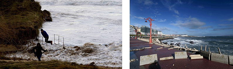
Figure 1. Left: people running away from the waves at Esteiro beach (Xove, Lugo, Northern Galicia) during the storm of February 2nd 2014 (Nadja storm). Source: La Voz de Galicia, photographer: Pepa Losada: http://www.lavozdegalicia.es/album/galicia/2014/02/02/danos-temporal/01101391328868511590785.htm. Right: impact on Coruña maritime promenade after the same Nadja storm. Source: El Ideal Gallego: http://www.elidealgallego.com/album/coruna/efectos-temporal-coruna/20140202182014171505.html.

The multi-parameter alert system worked well during these storms, providing red alerts (level 4) of wind waves, sea level and oscillations from all the existing buoys and tide gauges along the North Spanish coast, from Galicia to the Basque Country (see stations location in Figure 2). Significant wave heights and mean and peak periods at the buoys are displayed in Figure 3. Sea level oscillation warnings were also correctly issued, indicating that the tsunami detection algorithm was performing well. In the particular case of the storm of January 6th, we received additional red alerts of sea level oscillations from stations as far away as the Canary Islands.

FIGURE 2

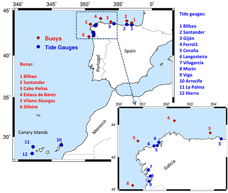
Figure 2. Position of the REDMAR tide gauges and Deep Water buoys from Puertos del Estado. Santander buoy belongs to the Spanish Oceanographic Institute.

FIGURE 3

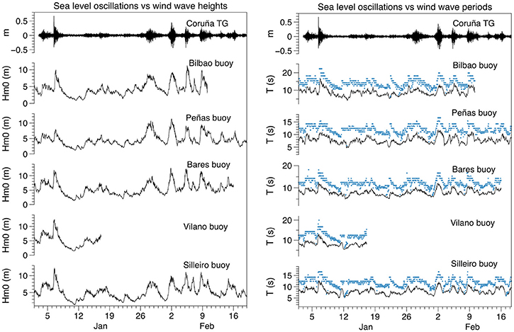
Figure 3. Significant wave height H_m0 (left) and periods (right: mean period T_m, black line, peak period T_p, blue dots) recorded in open waters by the PdE deep water buoys during the stormy period of January and February 2014. Sampling interval from the buoys is 1 h. Sea level oscillations (1 min high-pass filtered sea level) from Coruña tide gauge at the top of both plots for comparison: the larger oscillations occur during the extreme events of wind waves.

Observational Data

As can be seen in Figure 4 (left) the high-pass filtered 1-min time series from the tide gauges along the Spanish coast exhibit significant sea level oscillations simultaneously with this sequence of storms along almost all the coastline. A detailed study of the sea level data and a description of the atmospheric and oceanographic conditions during these days are presented below. The REDMAR tide gauges also provide information on wind waves recorded locally in the harbors and the significant wave heights (H_m0) from these are also displayed in Figure 4 (right). We can see that during these storms there were also important wind waves (0.4–1 m height is considered important inside a harbor) even at the quays where the tide gauge station is located. These wind waves (mostly swell) are usually a problem for harbor operations and confirm the critical situation at the coast and harbors these days: the local wind waves along with sea level oscillations and their associated currents may increase the damage to infrastructures and the possibility of flooding.

FIGURE 4

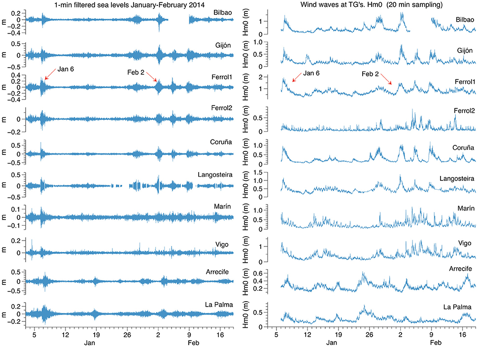
Figure 4. Left: 1 min high-pass filtered sea level data from the REDMAR network during the stormy period January- February 2014, showing the occurrence of significant high-frequency sea level oscillations along the Spanish coast; right: significant wave height (H_m0) computed by these Miros tide gauges for the same period.

These observed sea level oscillations are thought in principle to be “infragravity waves” generated by non-linear wave interactions of the incredibly high swell waves arriving at the coastline during these storms. The particularly long peak periods of the wind waves in open waters (Figure 3, right) make this event special and interesting: peak periods of up to 22.3 s were recorded at Bilbao buoy the 6th of January. Spectral analysis of the sea level time series should provide information, however, on the possibility of a “meteotsunami” generation as well. It is interesting to note the spatial scale of these events, along hundreds of kilometers of coast.

The largest sea level oscillations are observed on January 6th and February 2nd, as well as the most extreme wind waves recorded by the deep water buoys. During the first one, maximum significant wave heights of 12.4 m and 12.0 m were recorded by Vilano-Sisargas and Estaca de Bares buoys respectively (PdE, 2014). On February 2nd, however, the latter recorded an even larger significant wave height: 12.8 m, very close to its historical record (12.9 m). Maximum wave heights may be estimated roughly by multiplying these values by 1.6, which would result in individual wind waves of 20 m or more in open waters. This was confirmed by the delayed data processing of raw data from Estaca de Bares buoy, where an individual freak wave of 29 m height was found, becoming the highest wave height ever measured along the Spanish coast (M.I. Ruiz, personal communication). An alert level “4” for wind waves was issued by PdE alert system. As already mentioned these waves presented as well extremely long periods with peak periods reaching 22.3 s (Figure 3, right); this was a very distinctive characteristic of these storms, possibly related to the excited frequencies on the sea level oscillations, as will be shown later.

On both dates we also received level “4” alerts for sea level oscillations from most of the tide gauges shown in Figure 4; however, total sea level alerts (highs and lows) did not exceed level “2” on January 6th, and level “3” around February 2nd. This difference is due to the more precise coincidence of the second storm with the spring tide (Figure 5). In fact, this spring tide played a key role in the flooding, overtopping of waves and extreme sea levels recorded during this storm. The astronomical tide was particularly large that day due to the coincidence of the new moon and the lunar perigee (January 30th), its proximity to the perihelion (January 4th) and to zero lunar declination (February 2nd). Coincidence of lunar perigee and zero lunar declination occurs only every 6 years (Pugh, 2004).

FIGURE 5

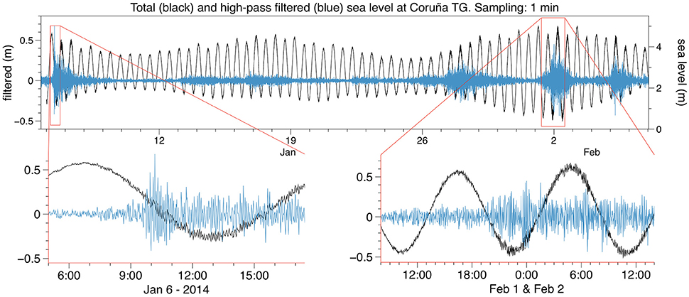
Figure 5. Total sea level (black) and high-pass filtered signal (blue) recorded by Coruña tide gauge for January–February 2014; data sampling: 1 min. The two most extreme events (January 6th and February 2nd) are shown amplified below. The maximum amplitude of the oscillation does not occur during high-tide, especially on January 6th.

Origin of the Oscillations

High frequency sea level oscillations were the second important contributor to the total extreme sea levels on these days. It is necessary to determine, first, the origin of these oscillations: in the absence of an earthquake and the coincidence with such big waves the first impression is that they are infragravity waves, very common in the Spanish Atlantic harbors, as already mentioned; nevertheless, they might also be meteotsunamis like those described in Frère et al. (2014). That paper described a meteotsunami event which occurred on June 26–28, 2011 in this region and which was recorded by all the tide gauges presented here, as well as at other stations from Portugal to England. It is interesting to notice the differences with our case: first, weather conditions in June 2011 were rather calm (summer time): wind waves at Peñas buoy (near Gijón tide gauge) were just around 1 m height between the 26th and 28th of June 2011. This is a typical situation during meteotsunamis on the Mediterranean Spanish coast, which usually occur in summer (Tintoré et al., 1988; Gomis et al., 1993; Monserrat et al., 2006b; Marcos et al., 2009). Second, analysis of the atmospheric pressure data from buoys and tide gauges revealed for this event that the oscillations occur when the atmospheric pressure is at a relative low level. This does not seem to be exactly the situation in 2014: Figure 6 shows that the larger sea level oscillations in our case are not exactly coincident with lower levels of pressure at the nearby deep water buoy. In fact, they seem to occur approximately 1 day later and coincide instead on February 2nd with a relatively higher value of pressure.

FIGURE 6

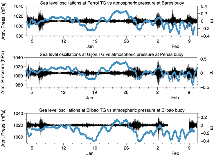
Figure 6. Sea level oscillations at Ferrol, Gijón, and Bilbao tide gauges for January–February 2014 (black lines), and atmospheric pressure recorded by the nearest deep water buoy (blue lines: Bares, Peñas, and Bilbao, respectively). Data sampling for sea level oscillations is 1 min, data sampling for atmospheric pressure recorded by buoys is 1 h.

Nevertheless, a meteotsunami could still have been generated for example by a sudden change in atmospheric pressure. Detection of fast atmospheric pressure jumps is usually difficult from existing meteorological networks as the sampling of most of the stations is too infrequent (10 min to 1 h). This is the case for the buoys of PdE network but also for others as described in Frère et al. (2014). The sampling interval of these buoys is 1 h, far from the 1 min temporal resolution required for implementation of future meteotsunami warning systems. As mentioned in previous section the REDMAR tide gauge network already takes into account this requirement and several microbarographs are now in operation with 1-min sampling and a resolution of 0.1 HPa (the resolution at the buoys is 1 HPa). In 2014 one of these sensors was already functioning at Vigo harbor tide gauge. Figure 7 (top) shows in detail the changes in atmospheric pressure recorded at this tide gauge on January 6th: although the resolution is clearly better than the one from the buoy (displayed also in the figure), it is difficult to conclude that there is a change capable of generating a meteotsunami. The relation of the oscillations with the sudden increase in wind waves is however more evident from middle and lower panels of Figure 7, which show the oscillations of sea level at Coruña plotted along with the wind waves significant wave height recorded by the nearest offshore buoy (Vilano) and by the tide gauge itself, respectively.

FIGURE 7

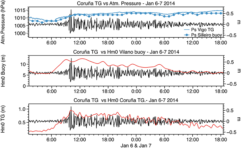
Figure 7. Sea level oscillations on January 6th 2014 at Coruña harbor vs.: top: atmospheric pressure data from Silleiro buoy (hourly values, blue dotted line) and from Vigo tide gauge (1 min values, blue line); middle: significant wave height recorded by Vilano buoy (red line); bottom: significant wave height recorded by Coruña tide gauge itself (red line). There is not atmospheric pressure data available from the nearest buoy (Vilano).

The amplitudes of these sea level oscillations (significant and maximum wave heights as explained in Section Data and Methods) are shown in the bottom panels of Figure 8 for La Coruña and La Palma tide gauges. Notice the resemblance of the peaks with the ones in significant wave height of wind waves in Figures 3, 4. This supports the idea of the swell wind waves being the forcing mechanism of these oscillations, which reach H_s and H_max of 0.5 and 0.9 m respectively in La Coruña, and of 0.3 and 0.5 m in La Palma, well far away from the center of the storms. Figure 8 (top panels) displays as well the spectrogram or temporal evolution of the spectra of 1 min data for these two stations (1536 points window with 128 points overlap): an increase in the energy content at higher frequencies (2 min or 0.5 cpm to 7 min or 0.15 cpm) is observed when each event starts. These periods are very close to the range of frequencies of the infragravity waves (30 s–5 min).

FIGURE 8

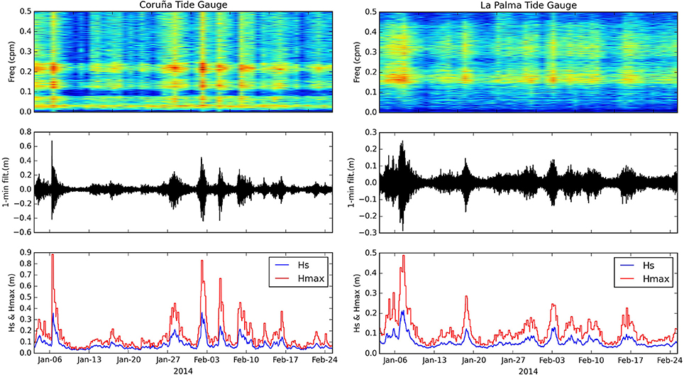
Figure 8. Top: spectrogram of 1 min high-pass filtered sea level data at Coruña (left) and La Palma (right) tide gauges, showing the daily variation of the spectra along the stormy period January–February 2014. Applied to 1536 points windows with 128 points overlap (colors in variance units). The storms coincide with the increase of energy on higher frequencies of sea level (periods 2′–6′); middle and bottom: 1 min high-pass filtered time series and estimated “seiche” amplitudes (half the significant wave height H_s and maximum wave height H_max) at these stations during this period (zero-crossing procedure).

We cannot discard the possibility of one of these frequencies being related to the excitation of the natural eigen periods at some harbors. Left panels on Figure 9 display for Coruña and La Palma tide gauges, the spectra for one specific day of 1 min data when maximum oscillations were recorded (red line) and the spectra for another day with no significant oscillations (blue line). The latter represent the spectral content of the background noise and therefore the natural frequencies or eigen periods of each location. A vertical logarithmic scale is used for an easier comparison of the two spectra. The frequency peaks on red and blue lines seem to be practically the same on both stations, what would confirm that we are observing an excitation of the natural eigen periods during the storm of January 6th, most evident at Coruña tide gauge.

FIGURE 9

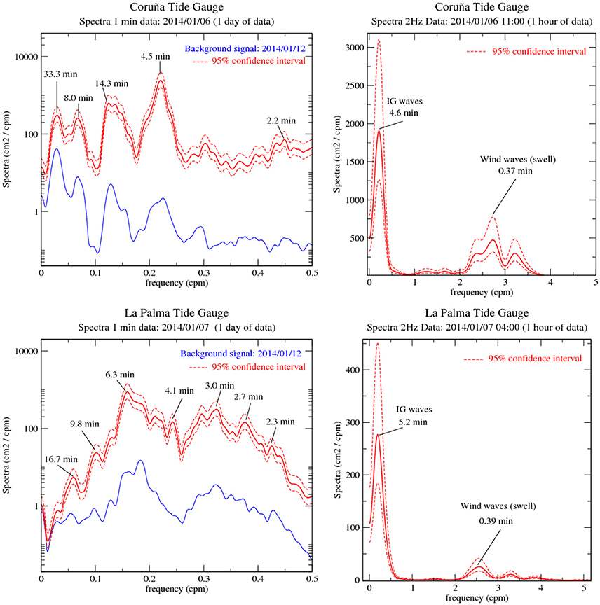
Figure 9. Spectral analysis for Coruña and La Palma tide gauges, during the storm of January 6–7, 2014. Left: spectra applied to 1 day of 1-min data, right: spectra applied to 1 hour of 2 Hz data. The 1- min and 2 Hz data have been high-pass filtered (periods <3 h and periods <45 min respectively). Red lines: spectra for 1 day/hour of maximum sea level oscillations (and 95% confidence intervals). Spectra from the background signal was added to the 1-min spectra (blue line) and a logarithmic vertical scale used in this case for easier comparison of the peaks. Spectra method: auto-covariance function smoothed with a Parzen lag window (40 degrees of freedom). Swell waves and infragravity waves are observed in the 2 Hz spectra.

Interestingly, Figure 8 (upper panel) shows a permanent signal in the range of 19–25 min (0.05–0.04 cpm) in the Coruña time series. It seems the signal is present before and after the increase of the oscillations amplitude and is also clear in the background noise spectra of 1 min data in Figure 9. This signal is not present or is very small in La Palma tide gauge (Canary Islands), but it is close to one found for the event of June 2011, on almost all the stations (Frère et al., 2014); this would discard a local topographic feature being responsible for this frequency peak although Frère et al. did not find a clear explanation about their origin. A spectrogram of the 1-min atmospheric pressure from Vigo tide gauge (not shown) revealed that this was the only band of frequencies with significant variance in the high temporal resolution atmospheric pressure data for all these weeks.

As the periods excited during 2014 events are very close to the Nyquist frequency of 1 min data (2 min), spectral analysis of the original 2 Hz data was performed also for the Coruña and La Palma tide gauge records during the storm of January 6th (Figure 9, right panels). In this case we have used a window of 1 h of data with maximum amplitude of the oscillations. The background noise at very high frequencies was so small that its spectra is not shown in this case. These 2 Hz spectra allow a clear distinction between the frequencies of the infragravity waves we are discussing here and the wind-waves at the tide gauge locations: we can see for the latter that most of the energy is concentrated on the swell band, with peaks at 0.37 min (22.2 s) and 0.39 min (23.4 s) for Coruña and La Palma, respectively. These very long peak periods are also present for this event at the open waters buoys, as already mentioned. This would explain therefore that associated infragravity waves were generated at a low frequency range, 4–6 min, and that their wave peaks were much narrower than usual for this particular event. According to the 1-min spectra (Figure 9, left panels), these waves were then further amplified at the resonance eigen periods at Coruña and La Palma, 4.5 min and about 6 min, respectively, becoming a peculiar and interesting case of resonance amplification of infragravity waves.

Contribution to Extreme Sea Levels

A better understanding of the contribution of these oscillations to total sea level is possible from the data presented in Table 1. Column 2 shows the maximum sea levels recorded by the tide gauges of Bilbao, Santander, Gijón, and Coruña during the storm of February 2nd, when the coastal inundation affected a largest area of the coast. These extreme sea levels are derived from the total 1-min sea level data. Column 3 contains the height of the tide at that instant, computed with the harmonic constants derived from harmonic analysis of more than one year of hourly sea level data in each harbor. The magnitude of the storm surge forecasted by the Nivmar system in operation at PdE is presented in column 4 for the point closer to each tide gauge, and column 5 contains the contribution from the “seiche” oscillation, estimated as half the significant wave height H_s (of the “seiche”) obtained in the way described in Section Data and Methods. The most important conclusion is that the extreme sea levels recorded during this event were significantly affected by these infragravity waves that had the same or even larger magnitude than the storm surge itself. In fact, the storm-surge component was rather moderate or small as was confirmed from analysis of the storm surge forecasted by the Nivmar system (the value forecasted for Coruña harbor was even negative). The addition of the values in columns 3, 4, and 5 is exactly the observed extreme value in column 2 for Santander and Gijón, and very close to it in Coruña and Bilbao (only 1 and 2 cm larger respectively).

TABLE 1

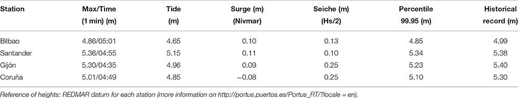
Table 1. Column 2: extreme total sea levels (m) / time (hh:mm GMT) recorded the 2nd of February by the tide gauges of Bilbao, Santander, Gijón and Coruña (sampling interval: 1 min); columns 3–5: contribution of the tide, surge and high frequency oscillation (considered here as half the significant wave height), the two latter at 05:00 GMT; columns 6 and 7: 99.95 percentile, and maximum sea level of the historical record (1992 to present).

The individual maximum wave heights (H_max of the “seiche”) recorded during this event reached 0.56 m in Bilbao, 0.45 m in Santander, 0.77 m in Gijón and 0.83 m in Coruña. The extreme sea level could have been larger in fact in Bilbao and Santander, as this maximum amplitude of the oscillations took place a couple of hours after the high tide in these harbors.

According to Table 1 we can see also that although the extreme high waters were below the historical record or maximum sea level recorded in each tide gauge since 1992, the 99.5 percentile of high waters was exceeded at all these harbors during this particular storm except at Coruña (precisely the one with a smallest storm surge component).

Therefore, the extreme sea level values recorded were in great part caused by the large spring tide added to a moderate or negligible storm surge, in combination with “seiches” of H_s reaching up to 0.5 m (0.25 m amplitude) in some cases. Since these oscillations are stochastic in nature, (and similar to wind waves in this sense) we need to take account of the probability of an individual maximum wave coinciding with the high tide.

Sea Level Data Recorded after the Atlantic Ridge Earthquake, February 13th, 2015

An earthquake with magnitude Mw = 7.1 took place in the middle of the Atlantic ridge on February 13th, 2015 at 18:59:12 (UTC). The earthquake epicenter was located at 52.649°N, 31.902°W, well within the Earthquake Source Zone monitored by the NEAMTWS Candidate Tsunami Service Providers (CTSP's). The exact position of the epicenter in this region determines the kind of message provided by the NEAMTWS CTSPs in the Atlantic; in this case it was in the region where messages must be issued for earthquakes with magnitude larger than 5.5.

In spite of the relatively high magnitude of the earthquake the focal mechanism was a strike-slip one in a transform fault (with centroid depth: 25.2 km, strike: 277, dip: 88, slip: −170, according to the Global Centroid Moment Tensor Catalog: Dziewonski et al., 1981; Ekström et al., 2012); a tsunami wave is not expected for this kind of earthquakes due to the lack of significant vertical movement of the ocean bottom. For this reason, NEAMTWS warning center provided just an information message for the region 12 min after the earthquake.

Interestingly, about 3 h after, a small increase of variability was observed in the 1-min filtered data from Langosteira tide gauge, a station located on the Northwest corner of the Spanish coast, at the external harbor of La Coruña (Figure 1). This signal could have been interpreted by mistake as the record of a small tsunami by a technician on duty on a tsunami warning center. In fact, this information was leaked out to press by an expert external to NEAMTWS and the National Tsunami Warning Center in Spain. The automatic algorithm for tsunami detection in PdE triggered an alert level “2” message for the station of Langosteira; the first alert was issued at 22:54:00 UTC, and several times thereafter until the morning of the 14th of February. It is important to stress that the thresholds of the algorithm are fixed according to the local variability of sea level at each harbor. As described in the previous section, oscillations similar to these ones are common along the North Spanish coast and are usually caused by wind waves in this region.

Looking for more tsunami signals after the earthquake of February 13th, 2015, a review was made through the IOC Sea Level Station Monitoring Facility (IOC/SLSMF) and other data portals such as the IBIROOS In-Situ Tac (that includes all in-situ marine observational platforms, including tide gauges, in the Atlantic European coast). A significant improvement on the availability of 1 min sea level time series during the last 10 years has been possible thanks to the new requirements established for tsunami warning: the percentage of tide gauges with 1 min sampling in this region has increased from 0% in 2006 to a 61% of the existing stations in 2015. As a result, records were available from the 50 locations shown in Figure 10 (left), with stations from Iceland (Reykjavik) to Cape Verde (Palmeira), and a couple of stations in the Canadian coast. Other stations on the US coastline and Canada that did not appear to display any significant signal or that had less frequent data sampling were not included in this analysis. Similarly, French stations are not included here as CEA (France) advised that a significant signal was not detected along the French coast.

FIGURE 10

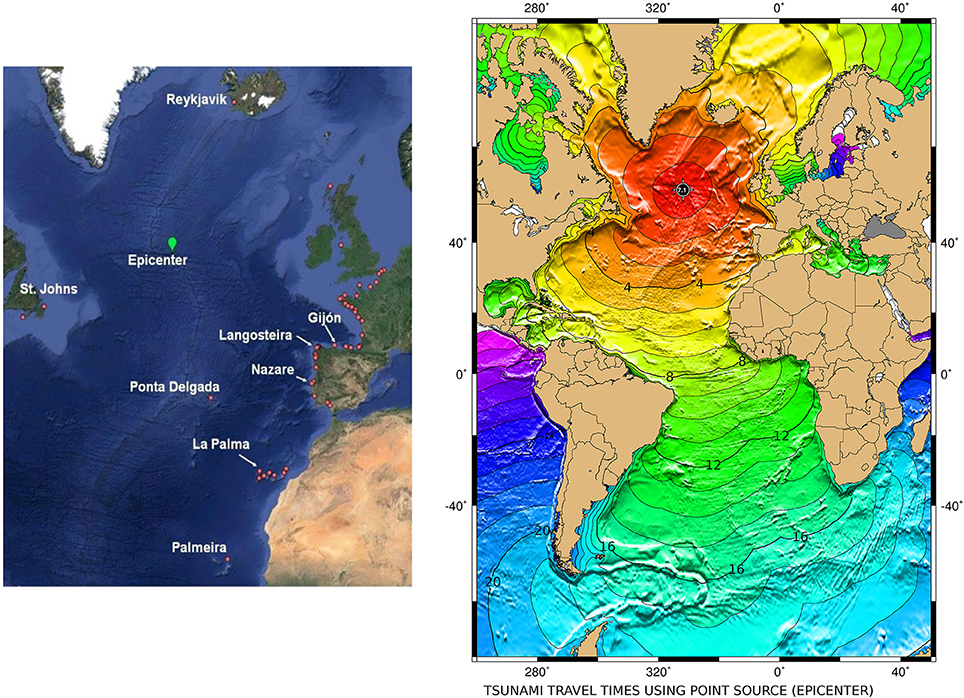
Figure 10. Left: up to 50 tide gauges (red dots) with 1-min data were available during the 13th of February 2015 earthquake event. Only a subset of them presented a possible small signal; the most evident was observed in Langosteira tide gauge; right: tsunami propagation (1 h contour line) generated at the epicenter of the earthquake of 13th February 2015, 18:59:12 UTC, in the Atlantic ridge, as provided by the model TTT SDK v3.3.

The filtered signal obtained from the rest of stations revealed different magnitudes of potentially normal variability at each harbor whilst those stations along the Iberian Peninsula North and North-West coasts displayed a possible earthquake-related signal. These stations were: Bilbao, Santander, Gijón, Coruña, Ferrol, and Langosteira, from the REDMAR network, and Peniche, Nazare, and Leixoes in the Portuguese coast, north of Lisbon. A possible signal could also be perceived at Reykjavik (Iceland) and Palmeira (Cape Vert). However, there were not significant oscillations in the filtered time series at the Canary Islands stations.

The arrival time of the potential tsunami wave was obtained by IGN for each tide gauge station from the numerical model TTT (Travel Time Software) SDK v3.3 (Table 2). The program calculates propagation velocities based on an input bathymetry grid and uses Huygens constructions to propagate the wave front from the epicenter to all nodes on the grid (Wessel, 2009). A map of this theoretical tsunami propagation time is shown in Figure 10 (right), with contour lines of 1 h.

TABLE 2

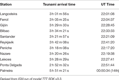
Table 2. Estimated arrival times of the first tsunami wave from numerical simulations of the earthquake of February 13th, 2015 in the Atlantic ridge.

The 1-min filtered sea level time series are displayed in Figure 11 for the subset of these 50 stations where a signal, however small, was found. The red line indicates the time of the earthquake. Expected arrival times from the numerical simulation presented in Table 2 have been added by means of vertical black arrows.

FIGURE 11

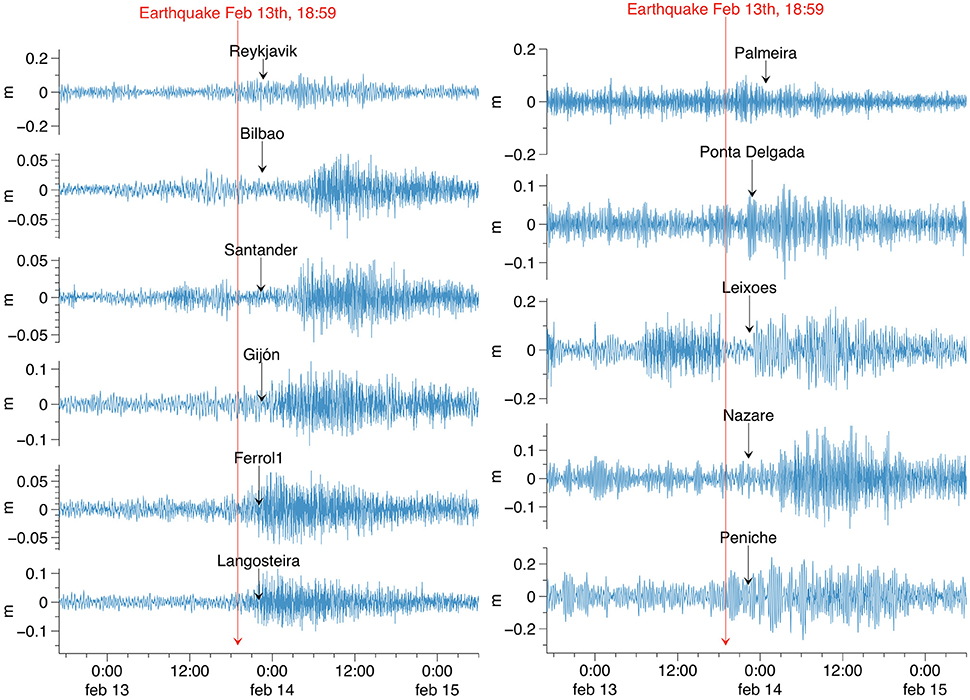
Figure 11. 1 min high-pass filtered sea level time series from those stations on Figure 10 where a signal, even if small, might be present after the earthquake of February 13th 2015 showing the expected arrival times in Table 2, derived from the tsunami propagation model, at each tide gauge (black arrows). The earthquake time is indicated by the red arrow.

These plots reveal, firstly, that there is no clear signal at most of the stations, if the times of earthquake and expected arrival of the wave are considered. The time series show a different behavior after the arrival time at all the stations except Palmeira, Ponta Delgada, and Reikjavik. In particular an increase of variability is observed immediately after or coincident with the arrival time only at Langosteira, Ferrol, Gijón, and Leixoes. Others show a signal several hours before or after the estimated arrival time.

It is difficult to determine clearly if a very small tsunami could have reached these tide gauges mainly for two reasons: (a) the uncertainty in the simulated arrival times could be large for those points where local bathymetry is not well resolved, (b) the local variability of each harbor and their relation to other oceano-meteorological reasons such as meteotsunamis or wind-waves.

Analysis of Langosteira Tide Gauge

It is interesting that, by chance or not, the increase of variability at this station coincides rather clearly with the expected arrival time from the model in this case, and that there is not significant energy during the day or few hours before the event.

Langosteira and Gijón 1 min high-pass filtered signals are displayed in Figure 12 along with their spectrogram and estimated amplitude. In this case the spectrogram was derived using a 512 points window (around 8 h) with a 128 points (2 h) overlap. It can be seen that the event recorded in Langosteira reflects not only a small increase of the magnitude of the signal, with waves reaching amplitudes of 10–15 cm, but also the appearance of higher frequency oscillations, with energy suddenly present at all the lower periods up to 2 or 2.5 min, as observed in the events of 2014 presented in previous section, along with the 15–25 min period signal already present before the event. Once again, it seems there is a kind of permanent background oscillation in this band of frequencies in this part of the Spanish coast, observed now also at Langosteira and Gijón tide gauges, similar to the one observed at Coruña during January–February 2014, and to the one found by Frère et al. (2014).

FIGURE 12

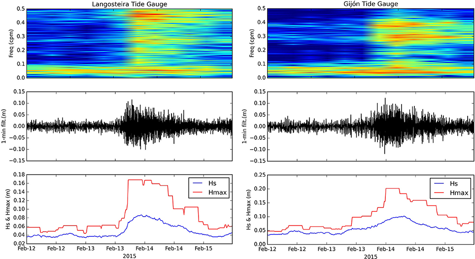
Figure 12. Top: spectrogram of 1 min high-pass filtered sea level data at Langosteira (left) and Gijón (right) tide gauges, showing the temporal evolution of the spectra along February 12–15th 2015. Applied to 512 points windows with 128 points overlap (colors in variance units). A constant signal with periods in the range of 15–25 min is present before the event at both stations; new signals for lower periods (until 2 or 2.5 min) appear when the event starts; middle and bottom: 1 min high-pass filtered time series and corresponding estimated “seiche” amplitude (half the significant wave height H_s and the maximum wave height H_max) during this period (zero-crossing procedure).

The daily spectra of 1-min data for 1 day before (12th of February) and 1 day after the event (15th of February) are displayed in Figure 13 (left panel), in the same way described for Figure 9 for January–February 2014. This figure confirms the previous statement that a signal with a period between 15 and 25 min is always present (peak on 17.2 min); the higher frequency oscillations (up to 2 min) are mostly excited during the event (red line). Notice the coincidence of this signal with the ones observed in previous section for Coruña tide gauge (nearby Langosteira). In that case the excitation of the lower periods seemed to be associated to the storms and huge wind waves; it could be the case also in this event.

FIGURE 13

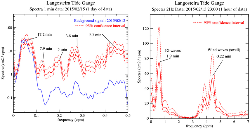
Figure 13. Left: spectral analysis of 1 min (left) and 2 Hz (right) data for Langosteira tide gauge on February 13th 2015. The 1-min and 2 Hz data have been high-pass filtered (periods <3 h and periods <45 min respectively). Red lines: spectra for 1 day/hour of maximum sea level oscillations (and 95% confidence intervals). Spectra from the background signal was added to the 1-min spectra (blue line) and a logarithmic vertical scale used in this case for easier comparison of the peaks: the energy at higher frequencies (e.g., periods of 3.6 and 2.3 min) increase significantly during this event. The 2 Hz spectrum reveals the energy content on the infragravity waves (peak very close to the Nyquist frequency of 1 min data) and on the swell bands. Spectra method: auto-covariance function smoothed with a Parzen lag window (40 degrees of freedom).

In the right panel of Figure 13 the spectral analysis of the 2 Hz data from Langosteira tide gauge is displayed (again in the same way as those in Figure 9). Here, the presence of a peak on the infragravity waves band is also clear, with a period of 1.9 min, clearly inside the infragravity frequency range. Wind waves swell are also present in this case with a peak period of 13.2 s (0.22 min), significantly lower, nevertheless, than in 2014 events, what would explain the lower period of this infragravity wave, most common according to the literature.

Although there were not extreme waves and storms during February 2015, their influence cannot be completely disregarded for Langosteira. Figure 14 shows the increase in significant wave height (up to 6.5 m) and mean period of the wind waves recorded at the nearby buoy of Estaca de Bares (offshore, north of Langosteira), during the appearance of the oscillations in this station. Based on the experience of other events, therefore, this sudden change in amplitude and period of the wind waves would be most likely the origin of the oscillations (infragravity waves) observed in this tide gauge coincidentally when a potential small tsunami could have reached the station. The 1 min meteorological data recorded at Vigo tide gauge during the same period also simply reflect an increase in the wind velocity at that time (related to wind waves on the other hand); the atmospheric pressure data does not show any relevant feature before February 13th, confirming the origin of the observed sea level oscillations in Langosteira in the infragravity waves.

FIGURE 14

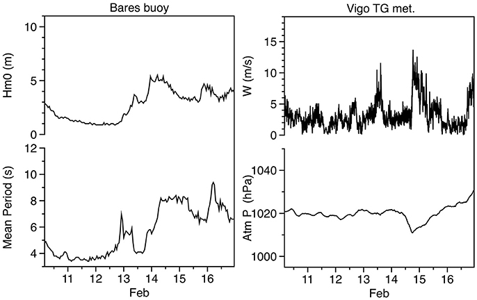
Figure 14. Left: significant wave height (H_m0) and mean period (T_m) recorded by Bares open waters buoy during the oscillations event of February 2015; right: mean wind velocity and atmospheric pressure recorded by the meteorological sensors of Vigo tide gauge for the same period (1-min sampling resolution).

The discussion above illustrates how considering these kind of signals as a small tsunami useful for validation of tsunami modeling without more careful analysis can be dangerous, and how the analysis of other environmental variables, as well as a better knowledge of the local sea level variability in the station, and the local response to the different forcings, is needed.

Discussion

Nowadays we are in a fortunate new position to improve our understanding of sea level oscillations at higher frequencies (periods of the order of minutes) thanks to significant changes in observational sea level networks. Detection of small tsunami signals at tide gauges is of great interest for assessing the skill of existing tsunami warning systems and for validation of tsunami propagation models, and this need is leading to the development of new methodologies of sea level data processing and automatic detection algorithms such as the ones described in this paper. However, the tsunami footprint on sea level records resembles other more frequent types of phenomena, already known and studied from an academic point of view, but not usually considered within sea level warning systems.

The analysis of the two events presented in this paper has provided several lessons. First of all, it reveals the importance of considering these oscillations for a more precise design of sea level alert systems. Although wave-setup is already considered of relevance for sea level forecasts and this may be solved by means of coupled wind-wave and storm surge models, additional sea level oscillations in the frequency of the “tsunami” signals should also be taken into account in the future. In the examples described in this paper the forcing of these oscillations seems to be mainly wind waves, but in other regions the forcing may be different (meteotsunamis such as the “rissaga” events in the Mediterranean Sea, for example). Case studies like this one will contribute to a better physical knowledge of all these phenomena.

Another important lesson from this study it that detection of small tsunamis from tide gauges is uncertain due to the inherent sea level variability caused by all these oceano-meteorological agents, but also due to errors in tsunami propagation models or problems in the data (transmission fails, spikes, etc). This leads to a continuous need for refinement of automatic algorithms based on the analysis of events like the ones described here.

The storms of January and February 2014 represent an example of real extreme events where both wind-waves and sea level, with their different components combined, and even without a significant storm surge, may cause severe damage and flooding in harbors and along the coastline. Therefore, future extreme analysis should consider this random process to determine maximum (and minimum) sea levels. The low sampling interval allows an adequate measurement of the effect of these oscillations in sea level records, which is the main reason for the upgrade of the tide gauge networks that in the past usually worked with 10 or 15 min sampling intervals at best. The sea level signals observed along the Spanish coast in January and February 2014 were not that different from the ones of a small tsunami.

The tsunami automatic detection algorithm in PdE performed perfectly well during these storms, providing red alerts for oscillations. The multi-parameter alert system provided as well red alerts for wind wave heights in open waters (although the most anomalous feature of these storms were the long peak periods), and yellow or orange alerts for total sea level. However, the sea level forecast did not reach the level of alert obtained from observations as it was based on just the forecast of the tide and the storm surge. This confirms the interest of the multi-hazard approach and the need for taking into account these physical phenomena in the future developments of the sea level forecasting system.

Concerning the observational network, in this paper we present the development of a new procedure for characterization of these oscillations in terms of amplitude and period. Initially implemented for the 1 min data submitted in real time in PdE, and tested with success in these two examples, the procedure needs to be improved and adapted to automatic processing of the original 2 Hz raw data. This is important especially for the periods of the infragravity waves, very close to the Nyquist frequency of 1 min data, as we have seen here, and will become possible as the network communications and access to these data improve in the future. A prototype is in fact already in operation for one tide gauge from the REDMAR network.

The Atlantic Ridge earthquake on 13th February 2015 was not expected to generate a tsunami signal; however, the occurrence of small oscillations in the North and West coast of the Iberian Peninsula revealed the complexity of interpretation of tide gauge data and the need for analysis of sea level in combination with other environmental variables. Although the signal observed in a few tide gauges is coherent with the expected arrival time of a small tsunami, and the wind waves at that time were not extreme, a detailed analysis has shown that these oscillations could be most likely infragravity waves and not a tsunami signal (spectral analysis of the time series reveals similar behavior of this event and the previous one).

Although we point to the wind waves as the main mechanism of the oscillations observed in these two examples, we cannot discard completely the possibility of a combination of effects and the occurrence as well of a meteotsunami, especially during one of the events of 2014. Considerable research has been done about these oscillations associated with atmospheric pressure disturbances in the last decades; the availability of microbarographs like those already in operation in the REDMAR network is expected to be of help in the establishment of future meteotsunami warning systems. These data could be integrated into these systems as the sea level data are already included in the tsunami warning systems. Although ideally offshore bottom pressure sensors would be more useful in both cases, the reality is that nowadays the only data available in real time for most of the countries in Europe are provided by tide gauges at the harbors, so it makes sense that we should improve the tools to use these data in near-real time and to interpret them correctly. Future work should focus therefore on more detailed studies of the local response of small bays and harbors to all these external forcings. This local knowledge will allow the design of more reliable and refined alert systems. This is the objective of future projects in PdE, that is starting now to pay more attention to the tremendous amount of 2 Hz and 1 min data recorded inside the Spanish harbors.

Finally, tsunami warning centers should be aware of these limitations and the complexity of the sea level measurements: once again, multi-hazard experts, with a combined knowledge of tsunamis, oceanography and meteorology, and making use of information from the whole network of stations (and not relying just on local information) will ensure reliable interpretation of the detection networks and a better understanding of the sea level risks taking into account all the different phenomena and the catastrophic consequences that their superposition may generate.

Author Contributions

BP: originator of the idea of the paper, manuscript writing; preparation of figures and tables, development of the algorithm for 1 min data processing, responsible of the sea level data processing in PdE including design of automatic quality control and alert issues. FM: implementation of an upgrade of the tsunami algorithm for tsunami detection in Java; generation of an offline Java script of this algorithm for easy application to the stations not included in the Portus system (Puertos del Estado). CG, JC, FS: tsunami wave arrival times at each station, description of the earthquake characteristics. EA: detailed review of the article, including re-writing of several sections and an improved description of the measurements during the storms of January–February 2014, with emphasis in the analysis of the storm surge, seiche and tide components.

Funding

PdE, Instituto Geográfico Nacional and CEA. SOPRANO project (Spanish national project: Plan Estatal de Investigación Científica) y Técnica y de Innovación 2013–2016 (Convocatoria 2014), Ministerio de Economía y Competitividad).

Conflict of Interest Statement

The authors declare that the research was conducted in the absence of any commercial or financial relationships that could be construed as a potential conflict of interest.

Acknowledgments

We wish to thank first all the operators and maintenance technicians of Puertos del Estado networks of tide gauges and buoys (Sidmar and Oceanor personnel, Marta de Alfonso and María Isabel Ruiz). We thank as well the Sea Level Station Monitoring Facility of the IOC (UNESCO), the IBIROOS In-Situ Tac and the different national operators for the provision of tide gauge data of non-Spanish stations for the event of February 13th 2015. The Tsunami Travel Time software (TTT SDK v 3.3) was developed by Dr. Paul Wessel (Geoware, http://www.geoware-online.com), and is used by the NOAA Pacific Tsunami Warning Center and licensed to NOAA/ITIC for redistribution. Finally, we would like to express our gratitude to Dr. Angela Hibert, who kindly accepted to read the manuscript and make suggestions to improve the English writing. This study has been performed in the framework of the Spanish funded project SOPRANO.

References

Alasset, P.-J., Hébert, H., Maouche, S., Calbini, V., and Meghraoui, M. (2006). The tsunami induced by the 2003 Zemmouri earthquake (MW= 6.9, Algeria): modelling and results. Geophys. J. Int. 166, 213–226. doi: 10.1111/j.1365-246X.2006.02912.x

CrossRef Full Text | Google Scholar

Álvarez-Fanjul, E., de Alfonso, M., Ruiz, M. I., Lopez, J. D., and Rodriguez, I. (2002). “Real time monitoring of Spanish coastal waters: the deep water network,” Proceedings of the Third International Conference on EuroGOOS (Athens).

Google Scholar

Álvarez-Fanjul, E., Pérez-Gómez, B., and Rodríguez, I. (2001). Nivmar: a storm surge forecasting system for Spanish waters. Sci. Mar. 65, 145–154. doi: 10.3989/scimar.2001.65s1145

CrossRef Full Text | Google Scholar

BBC (2014). UK Storms: Extreme Weather Caused Years of Erosion 21 February 2014. BBCNews Magazine. Available online at: http://www.bbc.com/news/uk-26277373 (Accessed February 2016).

Beltrami, G. M., Di Risio, M., and De Girolamo, P. (2011). “Chapter 27: Algorithms for automatic, real-time tsunami detection in sea level measurements,” in The Tsunami Threat-Research and Technology, ed N.-A. Moerner (InTech), 549–573. doi: 10.5772/13908

CrossRef Full Text

Bressan, L., Zaniboni, F., and Tinti, S. (2013). Calibration of a real-time tsunami detection algorithm for sites with no instrumental tsunami records: application to coastal tide-gauge stations in eastern Sicily, Italy. Nat. Hazards Earth Syst. Sci. 13, 3129–3144. doi: 10.5194/nhess-13-3129-2013

CrossRef Full Text | Google Scholar

Church, J. A., Gregory, J. M., Huybrechts, P., Kuhn, M., Lambeck, K., Nhuan, M. T., et al. (2001). “Changes in sea level,” in Climate Change: The Scientific Basis, eds J. T. Houghton, Y. Ding, D. J. Griggs, M. Noquer, P. J. van der Linden, X. Dai, K. Maskell, and C. A. Johnson (New York, NY: Cambridge University Press), 639–694.

Defant, A. (1961). Physical Oceanography, Vol. 2. Oxford: Pergamon Press.

Dziewonski, A. M., Chou, T.-A., and Woodhouse, J. H. (1981). Determination of earthquake source parameters from waveform data for studies of global and regional seismicity. J. Geophys. Res. 86, 2825–2852. doi: 10.1029/JB086iB04p02825

CrossRef Full Text | Google Scholar

Ekström, G., Nettles, M., and Dziewoński, A. M. (2012). The global CMT project 2004–2010: centroid-moment tensors for 13,017 earthquakes. Phys. Earth Planet. Inter. 200–201, 1–9. doi: 10.1016/j.pepi.2012.04.002

CrossRef Full Text | Google Scholar

El País (2014). El Temporal Provoca Olas Gigantes de Hasta 13 Metros de Altura en el Cantábrico. 3 February 2014. Available online at: http://elpais.com/elpais/2014/02/03/actualidad/1391412691_659227.html

Frère, A., Daubord, C., Gailler, A., and Hèbert, H. (2014). Sea level surges of June 2011 in the NE Atlantic Ocean: observations and possible interpretation. Nat. Hazards 74, 179–196. doi: 10.1007/s11069-014-1103-x

CrossRef Full Text | Google Scholar

Gómez-Lahoz, M., and Carretero-Albiach, J. C. (2005). Wave Forecasting at the Spanish Coasts. J. Atmos. Ocean Sci. 10, 389–405. doi: 10.1080/17417530601127522

CrossRef Full Text | Google Scholar

Gomis, D., Monserrat, S., and Tintoré, J. (1993). Pressure-forced seiches of large amplitude in inlets of the Balearic Islands. J. Geophys. Res. 98, 14437–14445. doi: 10.1029/93JC00623

CrossRef Full Text | Google Scholar

Herbers, T. H. C., Elgar, S., and Guza, R. T. (1995). Generation and propagation of infragravity waves. J. Geophys. Res. 100, 24863–24872. doi: 10.1029/95JC02680

CrossRef Full Text | Google Scholar

Hibiya, T., and Kajiura, K. (1982). Origin of the Abiki phenomenon (a kind of seiche) in Nagasaki Bay. J. Oceanogr. Soc. Jpn. 38, 172–182. doi: 10.1007/BF02110288

CrossRef Full Text | Google Scholar

IOC UNESCO (2007). North-East Atlantic, the Mediterranean and Connected Seas Tsunami Warning and Mitigation System, NEAMTWS, Implementation Plan. Technical report 73, Intergovernmental Oceanographic Commission.

Jansà, A., Monserrat, S., and Gomis, D. (2007). The rissaga of 15 June 2006 in Ciutadella (Menorca), a meteorological tsunami. Adv. Geosci. 12, 1–4. doi: 10.5194/adgeo-12-1-2007

CrossRef Full Text | Google Scholar

Jenkins, G. M., and Watts, D. G. (1968). Spectral Analysis and its Applications. San Francisco, CA: Holden Day.

Google Scholar

Longuet-Higgins, M. S., and Stewart, R. W. (1962). Radiation stress and mass transport in gravity waves, with application to “surf beats.” J. Fluid Mech. 13, 481–504. doi: 10.1017/S0022112062000877

CrossRef Full Text | Google Scholar

Marcos, M., Monserrat, S., Medina, R., Orfila, A., and Olabarrieta, M. (2009). External forcing of meteorological tsunamis at the coast of the Balearic Islands. Phys. Chem. Earth 34, 938–947. doi: 10.1016/j.pce.2009.10.001

CrossRef Full Text | Google Scholar

Monserrat, S., Vilibić, I., and Rabinovich, A. B. (2006a). Meteorological tsunamis: Atmospherically induced destructive ocean waves in the tsunami frequency band. Phys. Chem. Earth 34, 1035–1051. doi: 10.5194/nhess-6-1035-2006

CrossRef Full Text | Google Scholar

Monserrat, S., Gomis, D., Jansá, A., and Rabinovich, A. B. (2006b). Ciutadella harbour, Menorca, Spain, 15 June 2006 rissaga. Tsunami Newsletter 38, 5–7.

Munk, W. H. (1949). Surf beats. Eos. Trans. Am. Geophys. Un. 30, 849–859. doi: 10.1029/TR030i006p00849

CrossRef Full Text

Munk, W. H. (1962). Long Waves, in The Sea. New York, NY: J. Wiley.

Nomitsu, T. (1935). A theory of tsunamis and seiches produced by wind and barometric gradient. Mem. Coll. Sci. Imp. Univ. Kyoto A 18, 201–214.

Orlić, M. (1980). About a possible occurrence of the Proudman resonance in the Adriatic. Thalassia Jugo-slavica 16, 79–88.

Google Scholar

Pattiaratchi, C. B., and Wijeratne, E. M. S. (2015). Are meteotsunamis an underrated hazard? Philos. Trans. R. Soc. A 373, 1–23. doi: 10.1098/rsta.2014.0377

PubMed Abstract | CrossRef Full Text | Google Scholar

PdE (2014). Historical Information Available online at: Puertos del Estado website: http://portus.puertos.es/Portus_RT/?locale=en (Accessed February 2016).

Pérez-Gómez, B., Alvarez-Fanjul, E., Pérez, S., de Alfonso, M., and Vela, J. (2013). Use of tide gauge data in operational oceanography and sea level hazard warning systems. J. Oper. Oceanogr. 6, 1–18. doi: 10.1080/1755876X.2013.11020147

CrossRef Full Text

Pugh, D. T. (2004). Changing Sea Levels. Effects of Tides, Weather and Climate. Cambridge, UK: Cambridge University Press.

Google Scholar

Pugh, D. T., and Woodworth, P. L. (2014). Sea Level Science: Understanding Tides, Surges, Tsunamis and Mean Sea Level Changes. Cambridge, UK: Cambridge University Press.

Google Scholar

Rabinovich, A. B. (2009). “Seiches and harbour oscillations,” in Handbook of Coastal and Ocean Engineering, ed Y. C. Kim (Singapore: World Scientific Publishing Co), 193–236.

Google Scholar

Rabinovich, A. B., and Eblé, M. C. (2015). Deep-ocean measurements of tsunami waves. Pure Appl. Geophys. 172, 3281–3312. doi: 10.1007/s00024-015-1058-1

CrossRef Full Text | Google Scholar

Rabinovich, A. B., and Monserrat, S. (1996). Meteorological tsunamis near the Balearic and Kuril Islands: descriptive and statistical analysis. Nat. Hazards 13, 55–90. doi: 10.1007/BF00156506

CrossRef Full Text | Google Scholar

Rabinovich, A. B., Stroker, K., Thomson, R., and Davis, E. (2011). DARTs and CORK in cascadia basin: high-resolution observations of the 2004 Sumatra tsunami in the northeast Pacific. Geophys. Res. Lett. 38, L08607. doi: 10.1029/2011gl047026

CrossRef Full Text | Google Scholar

Rabinovich, A. B., Vilibić, I., and Tinti, S. (2009). Meteorological tsunamis: atmospherically induced destructive ocean waves in the tsunami frequency band. Phys. Chem. Earth 34, 891893. doi: 10.1016/j.pce.2009.10.006

CrossRef Full Text

Sahal, A., Roger, J., Allgeyer, S., Lemaire, B., Lavigne, F., Cedex, M., et al. (2009). The tsunami triggered by the 21 May 2003 Boumerdes-Zemmouri (Algeria) earthquake: field investigations on the French Mediterranean coast and tsunami modelling. Nat. Hazards Earth Syst. Sci. 9, 1823–1834. doi: 10.5194/nhess-9-1823-2009

CrossRef Full Text | Google Scholar

Šepić, J., Vilibić, I., Lafon, A., Macheboeuf, L., and Ivanovic, Z. (2015b). High-frequency sea level 512 oscillations in the Mediterranean and their connection to synoptic patterns. Prog. Oceanogr. 137, 284–298. doi: 10.1016/j.pocean.2015.07.005

CrossRef Full Text | Google Scholar

Šepić, J., Vilibić, I., Rabinovich, A. B., and Monserrat, S. (2015a). Widespread tsunami-like waves of 23-27 June in the Mediterranean and Black Seas generated by high-altitude atmospheric forcing. Sci. Rep. 5:11682. doi: 10.1038/srep11682

PubMed Abstract | CrossRef Full Text | Google Scholar

Sheremet, A. T., Staples, F., Ardhuin, S., and Suanez, Fichaut, B. (2014). Observations of large infragravity wave runup at Banneg Island, France. Geophys. Res. Lett. 41, 976–982. doi: 10.1002/2013GL058880

CrossRef Full Text | Google Scholar

Sibley, A., Cox, D., Long, D., Tappin, D., and Horseburgh, K. (2016). Meteorologically generated tsunami-like waves in the North Sea on 1/2 July 2015 and 28 May 2008. Weather 71, 68–74. doi: 10.1002/wea.2696

CrossRef Full Text | Google Scholar

Tappin, D., Sibley, A., Horsburgh, K., Daubord, C., Cox, D., and Long, D. (2013). The English channel tsunami of 27 June 2011 – a probable meteorological source. Weather 68, 144–152. doi: 10.1002/wea.2061

CrossRef Full Text | Google Scholar

Tintoré, J., Gomis, D., Alonso, S., and Wang, D. P. (1988). A theoretical study of large sea level oscillations in the Western Mediterranean. J. Geophys. Res. 93, 10797–10803.

Vela, J., Pérez-Gómez, B., González, M., Otero, L., Olabarrieta, M., Canals, M., et al. (2014). Tsunami Resonance in Palma Bay and Harbor, Majorca Island, as Induced by the 2003 Western Mediterranean Earthquake. J. Geol. 122, 165–182. doi: 10.1086/675256

CrossRef Full Text | Google Scholar

Vich, M. D. M., and Monserrat, S. (2009). Source spectrum for the Algerian tsunami of 21 May 2003 estimated from coastal tide gauge data. Geophys. Res. Lett. 36, 1–5. doi: 10.1029/2009GL039970

CrossRef Full Text | Google Scholar

Vilibić, I., Domijan, N., and Cupić, S. (2005). Wind versus air pressure seiche triggering in the Middle Adriatic coastal waters. J. Mar. Syst. 57, 189–200. doi: 10.1016/j.jmarsys.2005.04.007

CrossRef Full Text | Google Scholar

Vilibić, I., Monserrat, S., and Rabinovich, A. B. (2014). Meteorological tsunamis on the US East Coast and in other regions of the World Ocean. Nat. Hazards 74, 1–9. doi: 10.1007/s11069-014-1350-x

CrossRef Full Text | Google Scholar

Vilibić, I., Sepić, J., Rabinovich, A. B., and Monserrat, S. (2016). Modern approaches in meteotsunami research and early warning. Front. Mar. Sci. 3:57. doi: 10.3389/fmars.2016.00057

CrossRef Full Text | Google Scholar

Wessel, P. (2009). Analysis of observed and predicted tsunami travel times for the pacific and Indian Oceans. Pure Appl. Geophys. 166, 301–324. doi: 10.1007/s00024-008-0437-2

CrossRef Full Text | Google Scholar

Woodworth, P. L., and Blackman, D. L. (2002). Changes in extreme high waters at Liverpool since 1768. Int. J. Climatol. 22, 697–714. doi: 10.1002/joc.761

CrossRef Full Text | Google Scholar

Woodworth, P. L., and Blackman, D. L. (2004). Evidence for systematic changes in extreme high waters since the mid-1970s. J. Clim. 17, 1190–1197. doi: 10.1175/1520-0442(2004)017<1190:EFSCIE>2.0.CO;2

CrossRef Full Text | Google Scholar

Wu, J. K., and Liu, P. L.-F. (1990). Harbour excitations by incident wave groups. J. Fluid Mech. 217, 595–613. doi: 10.1017/S0022112090000866

CrossRef Full Text