An Intercomparison of Dissolved Iron Speciation at the Bermuda Atlantic Time-series Study (BATS) Site: Results from GEOTRACES Crossover Station A

Introduction

Iron (Fe) is an essential micronutrient, limiting phytoplankton growth in large regions of the surface ocean (de Baar et al., 2005; Boyd et al., 2007). The bioavailability of Fe to phytoplankton in the ocean is complicated by the limited supply of Fe from remote crustal sources (Tagliabue et al., 2014) and the overwhelming complexation of dissolved Fe (DFe) by organic ligands in seawater (Gledhill and Buck, 2012). Organic complexation allows Fe to overcome its low inorganic solubility in oxygenated seawater (Kuma et al., 1996; Liu and Millero, 2002), though the resulting Fe-organic ligand complexes require specialized uptake mechanisms for Fe acquisition (Maldonado et al., 2005; Hopkinson and Morel, 2009; Shaked and Lis, 2012). Most recently, the organic complexation of DFe in the Atlantic ocean was characterized in consecutive basin-scale studies of DFe speciation that overlapped at Crossover Station A at the Bermuda Atlantic Time-series Study site as part of the international GEOTRACES program (Buck et al., 2015; Gerringa et al., 2015).

Fe-binding ligand concentrations and their conditional stability constants in seawater are typically determined using competitive ligand exchange-adsorptive cathodic stripping voltammetry (CLE-AdCSV) techniques (Gledhill and van den Berg, 1994; Rue and Bruland, 1995; Croot and Johansson, 2000). These techniques involve equilibrating filtered and buffered seawater samples with a range of inorganic DFe additions and a single concentration addition of a well-characterized competing (or “added”) ligand before analysis of each titration point by AdCSV on a hanging mercury drop electrode. The sequence and equilibration times of added DFe and competing ligand vary across techniques (e.g., Buck et al., 2012; Gledhill and Buck, 2012). Titration data from AdCSV analyses are subsequently interpreted using a combination of linear and/or non-linear interpretation approaches to determine ambient Fe-binding ligand concentrations and conditional stability constants from each sample titration.

These ligands are commonly described by ligand classes, denoted L₁, L₂, …L_i, where L₁ is the strongest ligand class detected, L₂ weaker, etc. These ligand classes are operationally defined by their associated conditional stability constants ($K_{Fe{L}_i,F{e}^{\prime }}^{cond}$). In cases where only a single ligand class is detected, this notation is often simplified to L or L_T for ligand concentrations and for $K_{FeL,F{e}^{\prime }}^{cond}$ the associated conditional stability constant. In published datasets of DFe speciation, the reported values of log $K_{FeL,F{e}^{\prime }}^{cond}$, $K_{Fe{L}_1,F{e}^{\prime }}^{cond}$, and log $K_{Fe{L}_2,F{e}^{\prime }}^{cond}$ show considerable overlap, and it has been proposed that these ligand classes be defined by specific ranges in log $K_{Fe{L}_i,F{e}^{\prime }}^{cond}$ values (Gledhill and Buck, 2012). The complexation capacity or competition strength of these ligands is described by α_FeL, which is a function of the free (not bound to Fe, “excess”) ligand concentration ($\left[L_i^{\prime }\right]=\left[L_i\right]-\left[DFe\right]$) and associated stability constant (log $K_{Fe{L}_i,F{e}^{\prime }}^{cond}$) of all ligand classes present: ${\alpha }_{FeL}=\sum \left[L_i^{\prime }\right]*K_{Fe{L}_i,F{e}^{\prime }}^{cond}$.

Of these different ligand classes, stronger L₁-type ligands (log $K_{Fe{L}_1,F{e}^{\prime }}^{cond}$ > 12) and siderophores in particular have been shown to play a distinct role in Fe solubility (Cheah et al., 2003; Buck et al., 2007; Rijkenberg et al., 2008; Wagener et al., 2008; Aguilar-Islas et al., 2010; Mendez et al., 2010; Bundy et al., 2014; Fishwick et al., 2014), though characterizing more than one ligand class during the interpretation of CLE-AdCSV titration datasets is challenging (Hudson et al., 2003; Wu and Jin, 2009; Laglera et al., 2013). In addition to requiring sufficient titration points to quantify more than one ligand class with suitable error estimates, resolving multiple ligand classes also requires that the alpha coefficients of the proposed ligand classes are suitably different (Hudson et al., 2003; Wu and Jin, 2009) and larger than the center of the analytical window (α_FeL of the added competing ligand) employed (Laglera et al., 2013).

There are several CLE-AdCSV techniques for DFe speciation in seawater, which are typically defined by the choice of added competitive ligand employed for the titrations, though titration conditions (pH, temperature, concentration of added ligand, order and range of Fe and ligand additions, equilibration times) may also vary (Gledhill and Buck, 2012). The interpretation techniques used to obtain ligand concentrations and conditional stability constants from the titration data generated by CLE-AdCSV are diverse as well, and several new techniques have emerged recently (Sander et al., 2011; Laglera et al., 2013; Gerringa et al., 2014; Omanović et al., 2015). At this time, there are no established reference samples for DFe speciation, and intercomparison activities are a useful alternative for assessing how these different CLE-AdCSV approaches compare.

A field intercomparison study was previously conducted for DFe speciation at three depths in the central North Pacific as part of GEOTRACES intercalibration activities (Buck et al., 2012). In that study, each analyst applied their chosen CLE-AdCSV technique shipboard to samples collected from the same GO-Flo bottle for each of three depths, and final results were compared across the different analysts. Results of this initial intercalibration effort indicated the best agreement between analysts employing the same CLE-AdCSV and interpretation techniques. Distinctions between interpretation techniques were highlighted in part to explain poorer agreement between analysts using different approaches, though analysts did not exchange titration data or directly compare interpretation techniques (Buck et al., 2012). More recently, intercomparison exercises focused on interpretation techniques applied to estuarine (Laglera et al., 2013) and simulated (Pižeta et al., 2015) copper speciation data have found that the interpretation technique employed can have a dramatic impact on results reported from the same original titration data when the ligand characteristics for multiple ligand classes are analyzed.

Here we present a comparison of DFe speciation datasets generated from the GEOTRACES Crossover Station A at the Bermuda Atlantic Time-series Study (BATS) site as part of the Dutch and U.S. GEOTRACES expeditions in the North Atlantic in June, 2010 (Gerringa et al., 2015) and November, 2011 (Buck et al., 2015), respectively. In addition to comparing full water column datasets from BATS between the two occupations, we also report results of reinterpretation exercises conducted with the original titration data from both BATS profiles. The impact of the chosen sensitivity parameter on the final results from each interpretation approach was also compared between analysts in this exercise.

Materials and Methods

Sample Collection

Dissolved Fe (DFe) and DFe speciation samples were collected following stringent trace metal clean protocols, which are outlined in the GEOTRACES Cruise and Methods Manual (Cutter et al., 2010). At the GEOTRACES Crossover Station A, Bermuda Atlantic Time-series Study (BATS) site, full water column depth profile samples were collected first by the Dutch GEOTRACES program in June 2010 and subsequently by the U.S. GEOTRACES program in November 2011 (Figure 1). Specifics of sample collection and analyses between the two groups participating in this intercalibration are provided under the methods descriptions below.

FIGURE 1

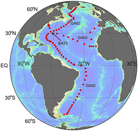
Figure 1. Map of stations sampled as part of GEOTRACES cruises GA02 and GA03. The Bermuda Atlantic Time-series Study (BATS) site, which serves as GEOTRACES Crossover Station A, is highlighted as the focus of this intercomparison study.

Dissolved Iron (DFe) Analyses

Total DFe concentrations are required for the interpretation of titrations for DFe speciation. The complete details of DFe analyses were published with the original basin-scale datasets (Rijkenberg et al., 2014; Sedwick et al., 2015). Briefly, in both cases, samples for DFe were collected separately from speciation samples in acid-cleaned low density polyethylene (LDPE) bottles. These samples were filtered through the same filters (<0.2 μm, see details below) used for the collection of speciation samples. DFe samples were acidified to 0.024 M hydrochloric acid (HCl) with high purity HCl (Johnson et al., 2007) and DFe concentrations were determined by flow injection analysis (FIA: Rijkenberg et al., 2014; Sedwick et al., 2015). Applying these analyses to reference standards from the SAFe (Johnson et al., 2007) and GEOTRACES programs resulted in DFe concentrations within the range of consensus values reported for each reference sample (Rijkenberg et al., 2014; Sedwick et al., 2015). Both of the DFe datasets used for DFe speciation calculations in this intercomparison were also included in the 2014 GEOTRACES Intermediate Data Product (Mawji et al., 2015).

2-(2-Thiazolylazo)-P-Cresol (TAC) Method

Filtered seawater (0.2 μm, Sartobran 300 cartridges) samples of 13 depths per station, representing the entire water column, were sampled on June 13, 2010 as part of the Dutch GEOTRACES program from an ultra-clean titanium depth sampler (de Baar et al., 2008). Samples from BATS were kept in a refrigerator (4°C) until analyzed shipboard between June 15 and June 17, 2010, within 4 days of sample collection.

TAC (2-(2-Thiazolylazo)-p-cresol) was used as a competing ligand to titrate the natural DFe-binding ligands by adding increasing concentrations of DFe to sub-samples. The bulk sample was buffered to a pH of 8.05 with 5 mM mixed ammonium-borate buffer cleaned of Fe using a TAC addition that was subsequently removed over a SEP-PAK column (Gerringa et al., 2015). The titrations consisted of 14 sub-samples with DFe additions of 0, 0.2, 0.4, 0.6, 0.8, 1, 1.2, 1.5, 2, 2.5, 3, 4, 6, and 8 nM Fe. The competing ligand “TAC” was used with a final concentration of 10 μM, resulting in α_Fe(TAC)2 of 251 as the center of the analytical window. The Fe(TAC)₂ complex was measured after equilibration (> 6 h) by adsorptive cathodic stripping voltammetry (AdCSV) (Croot and Johansson, 2000). Each of the 14 sub-samples was measured twice, resulting in a total of 28 titration data points.

The voltammetric equipment consisted of a μAutolab potentiostat (Type II and III, Ecochemie, The Netherlands), and a mercury drop electrode (model VA 663 from Metrohm) connected to a Metrohm-Applikon (778) sample changer. To prevent interference to analyses from motions of the ship, the electrode stand with the mercury drop electrode was stabilized on a wooden board hung with elastic bands inside an aluminum frame constructed at the Netherlands Institute for Sea Research (NIOZ). As a result, movements of the ship did not disturb measurements even during bad weather. All equipment was protected against electrical noise by a current filter (Fortress 750, Best Power).

During the course of the cruise, the TAC reagent used for analyses was found to contain relatively high Fe, resulting in an inadvertent addition of 0.5 nM Fe to the Crossover Station A/BATS profile samples (Gerringa et al., 2015). Thus, it is important to measure the Fe content in new batches of added competing ligands such as TAC since the quality with respect to Fe content was found to be variable between batches. The affected profile data from Crossover Station A/BATS was corrected by including this additional 0.5 nM Fe in the ambient DFe value used for titration data interpretation.

For the titration data interpretation a method was used in which the sensitivity (S), the conditional stability constant ($K_{Fe{L}_i,F{e}^{\prime }}^{cond}$), and the ligand concentration ([L_i]), are estimated using non-linear regression (Gerringa et al., 2014). By including S as an unknown parameter in the non-linear regression, S is corrected for the possibility that the visually linear part of the titration curve is still affected by unsaturated natural ligands. The non-linear regression method is simple to calculate, requiring easily available software (e.g., R) capable of least-squares regression or simplex regression, and calculates the standard errors (SE) of the fitted parameters. It is well-suited for the estimation of three or, if two ligand classes are assumed, five parameters out of a relatively small number of observations (Gerringa et al., 2014). At least four titration points per distinguished ligand group, together with a minimum of four titration points where the ligands are saturated, are necessary to obtain statistically reliable estimates of S, $K_{Fe{L}_i,F{e}^{\prime }}^{cond}$ and [L_i].

Salicylaldoxime (SA) Method

Depth profile samples collected as part of the U.S. GEOTRACES program were obtained using a trace metal clean sampling rosette deployed on a Kevlar line (Cutter and Bruland, 2012). For speciation samples, seawater was filtered through 0.2 μm Acropak (Pall Acropak 500) filters into acid-cleaned and Milli-Q (>18.2 MΩ cm)-filled narrow mouth fluorinated polyethylene bottles (FPE, Nalgene) that had been rinsed three times with sample prior to filling (Cutter et al., 2010; Buck et al., 2012). The speciation samples from Crossover Station A/BATS were collected on November 19, 2011, frozen at −20 °C and returned to the laboratory for analysis in June 2012. A total of 37 depths were sampled from this profile for DFe and DFe speciation.

Sample analyses for Fe-binding ligands using the SA method were conducted as described in Buck et al. (2015) on a BioAnalytical Systems (BASi) controlled growth mercury electrode (static drop setting, drop size 14) coupled to a BASi Epsilon ε2 voltammetric analyzer. Frozen speciation samples were thawed at room temperature, shaken, and distributed in 10-mL aliquots into lidded Teflon vials (Savillex) that had been previously conditioned with the expected Fe and SA additions in buffered Milli-Q. Each 10-mL sample aliquot was buffered to pH_NBS 8.2 with a chelexed-cleaned ammonium-borate buffer (Ellwood and van den Berg, 2001; Buck et al., 2007). Titrations consisted of 13 points: Two ambient (+0 nM Fe) measurements followed by ten dissolved Fe additions of +0.25, 0.5, 0.75, 1, 1.5, 2, 2.5, 3.5, 5, and 7.5 nM Fe. DFe additions were allowed to equilibrate with natural ligands in the samples for at least 2 h, or overnight at 4°C in the refrigerator (Buck et al., 2007). An addition of 25 μM SA (analytical window, α_FeSA = 79; Buck et al., 2007) to each titration vial was then made and allowed to equilibrate for at least 15 min prior to commencing AdCSV analyses (Rue and Bruland, 1995; Buck et al., 2007, 2015). Each titration point was analyzed once, generating a total of 12 points in each sample titration.

Titration data generated by CLE-AdCSV with SA was interpreted using a combination of van den Berg/Ružić and Scatchard linearization techniques (Scatchard, 1949; Ružić, 1982; van den Berg, 1982) as described previously (Rue and Bruland, 1995, 1997; Buck et al., 2007, 2012, 2015). In this approach, the sensitivity S for each sample titration was determined from the slope of the last few titration points. Results from the output of the two linearizations were then combined from each titration to determine averages for ligand concentrations and conditional stability constants (Buck et al., 2015). An inorganic side reaction coefficient for Fe of 10¹⁰ was employed when converting between log $K_{Fe{L}_i,F{e}^{\prime }}^{cond}$ and log $K_{Fe{L}_{i,}F{e}^{3+}}^{cond}$ notations of the conditional stability constant.

Intercomparison Activities

Dissolved Fe speciation results from separate occupations of Crossover Station A/BATS by independent analytical groups were compared in terms of dissolved Fe-binding ligand concentrations ([L_i]), their associated conditional stability constants ($K_{Fe{L}_i,F{e}^{\prime }}^{cond}$), and resulting organic complexation capacity (α_FeL, where ${\alpha }_{FeL}=\sum \left[L_i^{\prime }\right]*K_{Fe{L}_i,F{e}^{\prime }}^{cond}$ and $\left[L_i^{\prime }\right]=\left[L_i\right]-\left[DFe\right]$; see Gledhill and Buck, 2012 and references therein for additional information). These terms were determined by each group from a combination of analyzing samples by CLE-AdCSV to generate titration data and then mathematically deriving the Fe speciation terms from their titration data. The theory behind these interpretation techniques and visualizations of their application to natural samples can be found in the original literature for each method (Gerringa et al., 1995, 2014; Rue and Bruland, 1995) and in a recent interpretation intercalibration of idealized copper speciation data (Pižeta et al., 2015). In this intercomparison exercise, samples were not available for each group to conduct CLE-AdCSV analyses on the same samples. Instead, in addition to comparing final speciation results, the two groups exchanged CLE-AdCSV titration data from the BATS water column and then determined the organic complexation terms for the exchanged data using their own interpretation approach, which allowed a comparison of how interpretation technique influence profile speciation results. As part of this comparison of applying different interpretation techniques to exchanged titration data, the relative contribution of the sensitivity parameter chosen between interpretations was specifically addressed by either including a sensitivity value in the data exchange (“S given”) or not (“S determined”).

Altogether, there are three intercomparison activities reported here: (1) a comparison of reported Fe speciation results from GEOTRACES Crossover Station A/BATS; (2) a comparison of results derived from exchanging CLE-AdCSV titration data from the BATS water column for complete reinterpretation; and (3) a comparison of results after exchanging BATS titration data for the reinterpretation but given the sensitivity value determined by the original analyst for each dataset.

Results

As part of the Dutch and U.S. GEOTRACES programs, the organic complexation of dissolved Fe was determined through the entire water column of the Bermuda Atlantic Time-series Study (BATS) site twice, first in June 2010 (Gerringa et al., 2015) and again in November 2011 (Buck et al., 2015). Dissolved Fe concentrations differed through the water column between the two occupations (Figure 2A; Rijkenberg et al., 2014; Sedwick et al., 2015). In both cases, however, organic Fe-binding ligands were reported in excess of DFe concentrations throughout the water column, and thermodynamically stable (“strong”) organic DFe complexes were the dominant chemical form of DFe at all depths (Figures 2A–F; Buck et al., 2015; Gerringa et al., 2015).

FIGURE 2

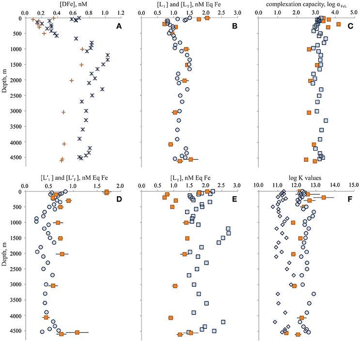
Figure 2. Dissolved iron (Fe) speciation results from the Dutch GEOTRACES GA02 BATS occupation in June 2010 (orange symbols) and from the U.S. GEOTRACES GA03 BATS occupation in November 2011 (blue symbols). (A) Dissolved Fe concentrations; (B) L₁-type (circles) and total (squares) ligand concentrations; (C) log complexation capacity of organic ligand pool; (D) excess L₁-type (circles) and excess total (squares) ligand concentrations; (E) total ligand concentrations; and (F) log conditional stability constants of L₁-type (circles), L₂-type (diamonds) and single (squares) ligand classes. Symbols for the results are specific to ligand class: circles for stronger L₁-type ligand class (2011 only), diamonds for weaker L₂-type ligand class (2011 only), and squares for total (2011) or single (2010) ligand characteristics. Concentration units for ligands are provided as nanomolar equivalents of DFe concentrations (nM Eq Fe). Conditional stability constants $K_{FeL,F{e}^{\prime }}^{cond}$ $K_{Fe{L}_i,F{e}^{\prime }}^{cond}$ and are presented as log K and log K_i, respectively, where i denotes ligand class (units of K: M⁻¹). Error bars represent standard errors of the reported results.

In June 2010, Gerringa et al. (2015) reported a single ligand class of total concentration range [L_T] = 0.72–2.05 nM Eq Fe (average: 1.25 ± 0.39 nM Eq Fe, n = 13) over the entire water column with an average log $K_{FeL,F{e}^{\prime }}^{cond}$ of 12.23 ± 0.49 (n = 13). In November 2011, Buck et al. (2015) reported two ligand classes at BATS. The stronger L₁-type ligand class was measured with very similar concentrations ([L₁] = 0.82–1.51 nM Eq Fe, average: 1.16 ± 0.21 nM Eq Fe, n = 37) and conditional stability constants (average log $K_{Fe{L}_1,F{e}^{\prime }}^{cond}$ = 12.42 ± 0.23, n = 37) to the single ligand class reported by Gerringa et al. (2015) for this station in June 2010 (Figure 2B). An additional weaker L₂-type ligand class (average log $K_{Fe{L}_2,F{e}^{\prime }}^{cond}$ = 11.28 ± 0.24) was also detected in these samples (Buck et al., 2015), leading to higher total ligand ([L_T] = [L₁] + [L₂]) concentrations (1.47–2.41 nM Eq Fe, average: 1.82 ± 0.24 nM Eq Fe, n = 37) in the November 2011 water column than reported by Gerringa et al. (2015; Figure 2E).

Excess ligand concentrations ($\left[L_T^{\prime }\right]=\left[L_T\right]-\left[DFe\right]$) were highest in the shallowest samples of the June 2010 profile (1.70 nM Eq Fe, n = 2) and averaged 0.71 ± 0.17 nM Eq Fe (n = 11) through the rest of the water column (Figure 2D). In the November 2011 profile, two ligand classes were determined. Excess L₁-type ligand concentrations ($\left[L_1^{\prime }\right]=\left[L_1\right]-\left[DFe\right]$)were also higher near the surface (0.72 ± 0.12 nM Eq Fe in upper 85 m, n = 4), in November 2011 and averaged 0.48 ± 0.13 nM Eq Fe through the rest of the water column (Figure 2D). Excess total ligand concentrations ([L′_T] = [L_T] − [DFe] = [L₁] + [L₂] − [DFe]) in November 2011 averaged 1.15 ± 0.26 nM Eq Fe through the water column. The elevated concentration of an especially strong ligand detected in the upper water column of the June 2010 profile contributed to higher organic complexation capacity (log α_FeL = 3.57 ± 0.33, n = 6) in the upper 500 m compared to deeper waters (log α_FeL = 2.76 ± 0.20, n = 7; Figure 2). Below 500 m, however, the measured complexation capacity was similar between the two occupations, if not slightly higher in the November 2011 profile (log α_FeL = 3.16 ± 0.18, n = 25; Figure 2C).

Reinterpretation Exercise

For the reinterpretation exercise, analysts exchanged CLE-AdCSV titration data and applied the interpretation technique used on their own data to the titration data received from the other group. Applying the combined van den Berg/Ružić and Scatchard linearization approaches (Rue and Bruland, 1995; Buck et al., 2012) to the June 2010 dataset resulted in similar [L_T] and log $K_{FeL,F{e}^{\prime }}^{cond}$ as reported from the original Gerringa et al. (2014)-based interpretation of the same data (Figures 3A,B). This agreement was even better when the sensitivity parameter given by Gerringa et al. (2015) was used in the reinterpretation (Figures 3C,D). Thus, in the case of the June 2010 dataset, both the original analyst and the reinterpretation results agreed that one ligand class was the best fit for these BATS titrations.

FIGURE 3

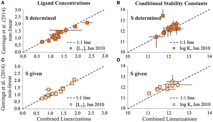
Figure 3. Results of the single ligand class reinterpretation exercises of the GA02 (June 2010) dataset for ligand concentrations (A,C; units: nM Eq Fe) and log conditional stability constants (B,D; units of K: M⁻¹). Results from the Combined Linearization approach to data interpretation are plotted on the x-axes vs. the results from the Gerringa et al. (2014) non-linear data interpretation approach on the y-axes. Upper panels depict results from when the sensitivity parameter (S) was determined in the reinterpretation exercise. Lower panels depict results of the reinterpretation exercise from when the S parameter was given by the original analyst.

This was not the case for the November 2011 dataset. The Gerringa et al. (2014) non-linear interpretation approach reported predominantly a single ligand class as the best fit to the November 2011 titration data (data not shown). Allowing the determination of two ligand classes from these titration data using this approach resulted in large standard deviations for the results (Figures 4A,B). However, as seen in the one ligand class reinterpretation, agreement between the average [L_i] and log $K_{Fe{L}_i,F{e}^{\prime }}^{cond}$ reported by the two interpretation techniques for this dataset was improved considerably by including the sensitivity value used in the original interpretation for the data exchange reinterpretation (Figures 4C,D). In the November 2011 titration data, curvature evident in the Scatchard plots was consistent with the presence of more than one ligand class (Rue and Bruland, 1995; Buck et al., 2012). The difficulty in quantifying a second ligand class in the Gerringa et al. (2014) non-linear interpretation of the 2011 data may in part reflect insufficient titration points in the interpretation limiting the degrees of freedom available to calculate the additional parameters required of two ligand classes with statistical certainty, regardless of whether the additional ligand class is present (Hudson et al., 2003; Wu and Jin, 2009; Gerringa et al., 2014).

FIGURE 4

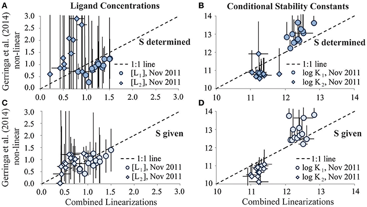
Figure 4. Results of the two ligand class reinterpretation exercises of the GA03 (Nov 2011) dataset for ligand concentrations (A,C; units: nM Eq Fe) and log conditional stability constants (B,D; units of K: M⁻¹). Results from the Combined Linearization approach to data interpretation are plotted on the x-axes vs. the results from the Gerringa et al. (2014) non-linear data interpretation approach on the y-axes. Stronger DFe-binding ligand results are represented by circles and weaker DFe-binding ligand results are represented by diamonds. Upper panels depict results from when the sensitivity parameter (S) was determined in the reinterpretation exercise. Lower panels depict results of the reinterpretation exercise from when the S parameter was given by the original analyst.

Discussion

Influence of Interpretation Approach on Fe Speciation Results

By swapping CLE-AdCSV titration datasets, analysts in this BATS intercomparison study were able to evaluate how the applied data interpretation approach influenced the speciation results. When determining a single ligand class from BATS titration data, the two interpretation approaches calculated similar ligand concentrations and conditional stability constants for that ligand class (Figure 4). Determining two ligand classes, as seen in the November 2011 titration dataset, was more challenging and resulted in poorer agreement between the interpretation approaches, especially for the second (weaker) ligand class (Figure 5). In particular, while the average ligand concentrations and conditional stability constants resulting from the two interpretation techniques approached each other, the standard deviations determined for these parameters by the Gerringa et al. (2014) technique were very large (Figure 5). This suggests that despite the curvature in the transformed Scatchard plot, the Gerringa et al. (2014) approach would determine a second ligand class from only 36% of the November 2011 samples.

FIGURE 5

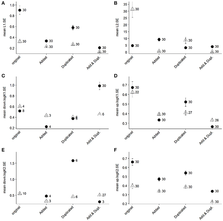
Figure 5. Mean standard error (SE) values of estimated ligand concentrations (“L_1,” A; “L_2,” B) and log conditional stability constants (“log K_1,” C,D; “log K_2,” E,F) of 30 repeated analyses using the Gerringa et al. (2014) non-linear fit for two ligand classes on titrations of two different samples from the GA03 occupation of the BATS site (2 m sample, closed circles; 96 m sample, open triangles). Two SE values were calculated for conditional stability constants (“up,” panels D,F; “down,” panels C,E) since the SE of the log values are not symmetrical (Gerringa et al., 2014). The “original” SE results represent the outcome of the interpretation using the original titration data. The influence of increasing the number of DFe additions (“Added”), duplicating measurements of original titration points (“Duplicated”), and both increasing the number of DFe additions and duplicating the measurements (“Add. & Dupl.”) was investigated in terms of standard errors of the data interpretation results. This was accomplished by artificially augmenting the original titration data with new DFe additions of 0.1, 0.35, 0.6, 2, 6, and 8.5 nM and duplicating these results following the error structure of the observed duplicates in the June 2010 titration data. The number noted next to each symbol represents the number of successful analyses out of the 30 attempted that resulted in a reportable value for SE.

The Gerringa et al. (2014) approach is mathematically robust, requiring at least twelve titration points to determine two ligand classes with confidence- four for each ligand class and four for the linear section of the titration curve to determine sensitivity (Gerringa et al., 2014). The combined linearization approach applied to the November 2011 dataset was not limited by this data structure, as this more traditional technique does not incorporate error calculations in the determination of speciation parameters. Instead, the average and standard deviation of the output from the two linearization techniques (van den Berg/Ružić, Scatchard) has previously been reported from studies using this data interpretation approach (e.g., Buck et al., 2012). However, since the two linearizations are not independent for a given titration dataset and the data fitting errors cannot be taken into account, the standard deviations of their averaged results underestimates the error in the interpretation. Most recently, the average parameter values from the combined linearizations were reported, and standard deviations were reserved to reflect the reproducibility of results derived from multiple independent titrations rather than quality of the titration data fitting (Buck et al., 2015).

In the Gerringa et al. (2014) paper, the authors evaluated the influence of numbers of titration points on derived standard deviations for the speciation parameters (see Figure 5 in Gerringa et al., 2014). In that case, the focus was on determining a single ligand class. It seems clear in the intercomparison here that there were insufficient titration points in the November 2011 dataset to allow for a robust determination of two ligand classes from the data. These titrations consisted of twelve DFe additions, the minimum number recommended for two ligand class determinations in the non-linear transformations (Wu and Jin, 2009; Gerringa et al., 2014). Yet titrating the excess strong DFe-binding ligands that were present in most of the November BATS samples with the first few DFe additions in the analyses left no measurable Fe bound to the added ligand (i.e., FeSA) at the beginning of the titrations, reducing the number of data points available for the interpretation to fewer than twelve.

Moving forward, the Gerringa et al. (2014) and similarly robust data interpretation techniques (Sander et al., 2011; Omanović et al., 2015) are preferred approaches to deriving metal speciation parameters from titration data (Pižeta et al., 2015). Accompanying this shift in interpretation approaches, titration datasets will require more individual data points to allow for the determination of more than one ligand class. This can be accomplished by increasing the number of DFe additions used in the titrations, by analyzing the different DFe additions more than once, or by doing both. Using representative titrations from the November 2011 BATS dataset, we investigated each of these potential modes of increasing titrations points on the standard deviations of results for two ligand classes derived from the Gerringa et al. (2014) approach for data interpretation.

Results of this assessment indicated that the combination of both increasing number of DFe additions and duplicating each titration point measurement resulted in the lowest standard errors for ligand concentrations and conditional stability constants (Figure 5). Increasing the number of unique DFe additions considerably reduced the standard errors of the results (Figure 5). In practice, however, it can be challenging to anticipate where in the titrations to incorporate these additions as well as to implement sufficient resolution of DFe additions in the curved section of the titrations when excess ligand concentrations are low. Correspondingly, duplicating the measurement of existing DFe additions may be a more practical approach to increasing titration data points, though this approach was not as consistent in improving the precision of results (Figure 5). It might also be necessary in some cases to be satisfied with unknown or relatively large SE values of estimated parameters or with acknowledging that an additional ligand class probably exists (e.g., when curvature in Scatchard plots is evident) without having sufficient data resolution to resolve the [L_i] or $K_{Fe{L}_i,F{e}^{\prime }}^{cond}$ values.

Overall, the observation of one or two ligand classes in the GEOTRACES BATS datasets for DFe speciation did not result solely from the different interpretation approaches applied. This is evident from the reinterpretation of the June 2010 titration data- applying the combined linearization approach did not elucidate a second ligand class in that data. Instead, the one or two ligand class characteristics of the BATS samples originates from the CLE-AdCSV titrations, with curvature in the November 2011 25 μM SA Scatchard plots supporting the presence of a second ligand class in those samples. Where interpretation approach clearly did play a role in the determination of one or two ligand classes was in the reinterpretation of the November 2011 datasets. Regardless of whether two ligand classes were indeed present, the number of data points in those titrations was insufficient to allow the robust determination of two ligand classes using the Gerringa et al. (2014) approach, evident in the large standard deviations of calculated results (Figures 4A–D).

The Particular Importance of the Sensitivity Parameter in Data Interpretation

In the BATS reinterpretation exercises, agreement of results from the different interpretation techniques applied to a given titration dataset was improved considerably by incorporating the sensitivity parameter value from the original interpretation for use in the reinterpretation (Figures 3, 4). These observations highlight the relatively large influence of the sensitivity parameter in titration data interpretation, which is consistent with the results of a previous intercomparison of interpretation approaches for dissolved copper speciation datasets (Pižeta et al., 2015). Surprisingly, when comparing the sensitivity parameter values derived from the two interpretation approaches in the BATS reinterpretation exercises, there were usually not large differences between the sensitivity values (Figures 6A,B). This suggests that even small changes in the sensitivity parameter determined can exert a disproportionate influence on results from the data interpretation. As with all parameters derived from the interpretation of titration data, higher resolution within titration datasets is likely the best way to constrain the determination of this important parameter.

FIGURE 6

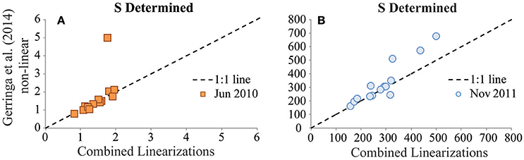
Figure 6. Values of the sensitivity (S) parameter determined for the GA02 (June 2010) dataset (A, units: nA nM⁻¹) and for the GA03 (Nov 2011) dataset (B, units: nA nM⁻¹). S values determined from the Combined Linearization approach to data interpretation are plotted on the x-axes vs. the results from the Gerringa et al. (2014) non-linear data interpretation approach on the y-axes.

SA, TAC, Suwannee River Fulvic Acid-Type DFe-Binding Ligands, and Analytical Windows

The identification of an additional, weaker ligand class in the 25 μM SA results of the BATS intercomparison exercise appears consistent with the results of a previous intercomparison of DFe speciation techniques conducted as part of the GEOTRACES intercalibration efforts in the central North Pacific (SAFe station) (Buck et al., 2012). In that effort, analysts conducted shipboard DFe speciation measurements on samples collected from three depths: 125 m (deep chlorophyll max), 1000 and 3000 m. The analysts employing CLE-AdCSV techniques with 10 μM TAC (α_Fe(TAC)2 = 250) and 25 μM SA (α_FeSA = 79), the same analytical windows employed for the BATS intercomparison here, showed the best agreement in determined ligand concentrations in the 125 m sample. In the 1000 and 3000 m samples, on the other hand, the 10 μM TAC measurements determined roughly half the ligand concentrations measured by the 25 μM SA methods (Buck et al., 2012). Only a single ligand class was reported by all participants in the North Pacific intercomparison, but the curvature of the titration data and the higher ligand concentrations and lower conditional stability constants determined by the 25 μM SA groups were consistent with the 25 μM SA method measuring weaker ligands not determined in the 10 μM TAC analyses.

The influence of freezing DFe speciation samples was also investigated in the previous North Pacific intercomparison exercise (Buck et al., 2012). No significant difference was found in that study between the DFe speciation results from samples analyzed before freezing and after freezing at −20°C, and only one ligand class was identified in all cases (Buck et al., 2012). In the BATS intercomparison, samples collected in November 2011 were stored frozen at −20°C prior to laboratory-based analyses while the samples collected in June 2010 were analyzed shipboard. Given the results of the North Pacific intercomparison (Buck et al., 2012) and the similar observations from an assessment of freezing DFe speciation samples conducted as part of the U.S. GEOTRACES program in the Atlantic (Buck unpublished), the differences in sample storage does not appear to be the best explanation for the presence of an additional weaker DFe-binding ligand class in the November 2011 BATS profile.

In the North Pacific intercomparison, the discrepancy in ligand concentrations and conditional stability constants between the 25 μM SA and the 10 μM TAC results was attributed in part to the presence of humic-type DFe-binding substances (Buck et al., 2012), which were measured at depth at the same central North Pacific station (Laglera and van den Berg, 2009). Humic-type substances, as represented by a Suwannee River Fulvic Acid (SRFA) standard (Arakawa and Aluwihare, 2015) in AdCSV studies (Laglera et al., 2007), have been shown to serve as an L₂-type DFe-binding ligand in the coastal Atlantic and the deep Pacific (Laglera and van den Berg, 2009). Of particular relevance to these intercomparison activities, the SRFA standard used to represent these DFe-binding humic substances is masked in CLE-AdCSV measurements made using TAC as the added ligand (Laglera et al., 2011). That is not to say that TAC analyses miss all DFe-binding humic substances, as elevated L₂-type ligand (log K = 11–12) concentrations measured in Arctic outflow waters by TAC were attributed to likely humic-binding substances (Gerringa et al., 2015). However, if DFe-binding ligands analogous to SRFA humic-type substances are present in the BATS samples, they may have been missed by the TAC analyses in June 2010. Indeed, the weaker DFe-binding ligand class determined in the November 2011 dataset had an average conditional stability constant of 11.28 ± 0.24 (n = 37), similar to the conditional stability constant determined for SRFA in seawater (11.0, Laglera and van den Berg, 2009).

Finally, the different analytical windows applied by the two groups likely also contributed to the detection of a weaker ligand class of Fe-binding ligands in the 25 μM SA (α_FeSA = 79) analyses that was not detectable in the 10 μM TAC (α_Fe(TAC)2 = 250) analyses. The influence of analytical window on speciation results has long been established for copper speciation analyses (Bruland et al., 2000; Buck and Bruland, 2005), where higher analytical windows measure lower concentrations of stronger (i.e., higher conditional stability constant) ligands than lower analytical windows (Bruland et al., 2000). In the Fe speciation measurements at BATS, however, comparable concentrations of the strongest ligand class were determined by both analytical windows while an additional weaker ligand class was determined in the lower analytical window. This apparent discrepancy between the Fe and Cu speciation intercalibrations across analytical windows may simply reflect the different ranges in analytical windows employed- the range is much smaller for Fe (α_FeAL = 79–250 = 10^1.9–10^2.4, this study) than for Cu (α_CuAL = 10^2.5–10^6.5, Bruland et al., 2000). Recent applications of multiple analytical windows for Fe speciation analyses using SA actually depict similar trends as seen in the BATS intercalibration, with lower analytical windows (α_FeSA = 30, 60) identifying weaker Fe-binding ligand classes than higher (α_FeSA = 100, 250) analytical windows (Bundy et al., 2014, 2015). The application of a lower TAC analytical window has also been shown to result in detection of weaker Fe-binding ligands (Gerringa et al., 2007).

The Speciation of DFe at BATS

Discrepancies in organic complexation results between individual datasets may reflect real seasonal changes at the BATS sampling site, particularly in the upper water column, as has been observed for DFe concentrations (Sedwick et al., 2005). Indeed, the DFe concentrations were quite different between the two GEOTRACES occupations of BATS/GEOTRACES Crossover Station A (Figure 2A; Rijkenberg et al., 2014; Buck et al., 2015; Gerringa et al., 2015; Sedwick et al., 2015). The analytical methods used for the DFe analyses were very similar (Rijkenberg et al., 2014; Buck et al., 2015; Sedwick et al., 2015) and the DFe concentrations results from the two occupations were successfully intercalibrated and were included in the GEOTRACES Intermediate Data Product (Mawji et al., 2015). Thus, the higher DFe in November 2011 compared to June 2010 in the upper water column may reflect the deposition of North American aerosols with higher fractional solubility of Fe at BATS in the late fall/early winter compared to the predominant deposition of relatively insoluble Saharan dust in the summer months (Sedwick et al., 2007). Previous studies indicate that particles, whether atmospheric, authigenic, biological or resuspended, can greatly influence DFe concentrations and size fractionation in the surface ocean (Sedwick et al., 2005; Buck et al., 2010a,b; Fitzsimmons et al., 2015), and that these influences are largely mediated by the concentrations and conditional stability constants of Fe-binding organic ligands in the water column (Rijkenberg et al., 2008; Wagener et al., 2008; Aguilar-Islas et al., 2010; Boyd et al., 2010; Bundy et al., 2014; Fishwick et al., 2014). The trend of higher DFe in the November 2011 water column was not restricted to the surface ocean though (Figure 2A) and we cannot explain these differences in deeper water masses from seasonality.

The higher DFe in the November 2011 profile at BATS would be expected to influence Fe speciation characteristics depending on the speciation of the DFe increase. The addition of DFe bound to a strong organic ligand (i.e., FeL₁) would increase the concentrations of DFe, L₁ and L_T, while excess ligand ($L_1^{\prime }$ and $L_T^{\prime }$) concentrations would remain unchanged. On the other hand, the addition of free (inorganic) DFe would titrate ambient stronger ligands (Rijkenberg et al., 2008), decreasing excess ligand concentrations while total ligand concentrations stayed the same. This last case is more consistent with the BATS results, where the total concentrations of stronger L₁-type ligands were most similar between the two occupations, and average excess stronger ligand concentrations were generally lower in the November 2011 profile with higher DFe. Thus, the difference in DFe between these profiles may represent an addition of inorganic Fe or weakly organically complexed Fe (i.e., FeL₂) to the November 2011 profile, analogous to the dissolution of particulate Fe by ambient strong Fe-binding ligands in the water column or samplers. If the difference in DFe concentrations between the two profiles is simply the result of an analytical offset, however, total ligand concentrations would be affected more than excess ligand concentrations since the change in DFe would not be “seen” by the added ligand (Thuróczy et al., 2010; Gledhill and Buck, 2012). Overall, because DFe is used in the calculation of ligand characteristics and samples were not exchanged for speciation analysis at the different analytical windows applied, it is challenging to delineate between the influences of analytical approach and DFe on the speciation results.

The contamination of TAC with DFe in the June 2010 analyses also complicated the speciation analyses, and in particular the distinction of two ligands. The inadvertently higher first DFe addition from the contamination of TAC may have masked any curvature in the titrations and resulted in loss of information right at the start of these titrations, where the strongest ligand class is typically characterized. However, this bias is not evident in the intercomparison results. The two profiles agreed best on the concentrations of the strongest DFe-binding ligands (Figure 2B), indicating that this strongest ligand class was well-characterized by the two occupations despite the different DFe concentrations between them and the DFe contamination in TAC. Instead, where the two datasets primarily differed was in the total concentrations of ligands measured, with the November 2011 dataset reporting an additional weaker ligand class in excess of DFe, which was not determined in the June 2010 profile. As noted above, the identification of a weaker ligand class in the November 2011 BATS profile likely derives from the different analytical windows applied and from the ability of the salicylaldoxime technique to measure Suwannee River Fulvic Acid (SRFA)-type ligands, which in turn may provide insight into DFe-binding ligand identity in these waters (Laglera and van den Berg, 2009; Laglera et al., 2011).

Beyond the differences in total ligand concentrations resulting from the presence of a weaker ligand class in one of the two BATS profiles, some seasonality may be evinced by differences in the strongest DFe-binding ligands, which otherwise compared well between occupations (Figure 2B). For example, in the upper water column, and in particular near the surface of the profiles, the stronger DFe-binding organic ligand concentrations were higher, with higher conditional stability constants, in the June 2010 profile compared to November 2011 (Figures 2B,F). These higher strong ligand concentrations resulted in a nearly order of magnitude higher DFe complexation capacity (α_FeL) in the upper 500 m of the water column in June 2010 (Figure 2C). Below 500 m and through the rest of the water column, log α_FeL was higher in the November 2011 profile (Figure 2C), reflecting the additional complexation capacity gained from the weaker ligand class determined in those samples. This weaker ligand class was also present in the upper water column samples of the November 2011 profile, though clearly the strongest DFe-binding ligands dominated organic complexation capacity of DFe in these waters.

Conclusions

The two occupations of the GEOTRACES Crossover Station A at the Bermuda Atlantic Time-series Study (BATS) site highlight the ubiquitous presence of organic DFe-binding ligands in the North Atlantic water column. The two analytical approaches showed excellent agreement in characterizing the strongest DFe-binding organic ligands throughout the profiles, independent of the considerable differences in DFe concentrations or the different CLE-AdCSV and data interpretation approaches between the two occupations. Given the importance of the strongest DFe-binding organic ligands in complexing ambient DFe and governing DFe cycling processes, these results are encouraging for continued integration of organic complexation datasets. A primary distinction in speciation results between the two datasets is the presence of a second weaker DFe-binding ligand class identified in the November 2011 profile that was not characterized in the June 2010 profile. Independent studies of humic-type substances suggest that this discrepancy may reflect a difference in the abilities of the added ligands employed in the CLE-AdCSV measurements to detect Suwannee River Fulvic Acid-type DFe-binding ligands in seawater. If this is indeed the case, it suggests that these SRFA-type ligands are a component of the weaker DFe-binding ligand pool at BATS, though it is also clear that the strongest DFe-binding organic ligands dominate the organic complexation capacity in these profiles. The lower analytical window applied to the November 2011 speciation analyses may also have contributed to the detection of a weaker ligand class in that profile.

In swapping CLE-AdCSV titration data and conducting reinterpretation exercises between the two groups, it became apparent that the number of number of titration points and the sensitivity parameter values employed in the interpretation substantially influenced the DFe speciation results calculated from a given titration. As was already concluded by Gerringa et al. (2014), without a suitable number of titration data points, interpretation techniques that take into account data fitting errors either will not allow characterization of more than one ligand class and/or will return high standard errors of the results, both resulting from inadequate data structure (degrees of freedom) provided by the titration data. Correspondingly, increasing the number of DFe additions in CLE-AdCSV analyses to generate at least 12 non-zero titration data points whenever possible and even duplicating titration data analyses can substantially increase precision in calculated results. The emergence of new and increasingly robust data interpretation techniques for speciation measurements allows for increasingly precise characterizations of the DFe-binding ligand pool in the oceans, and facilitating the availability of CLE-AdCSV titration datasets for use in reinterpretation exercises is encouraged to continue development in this area. Including the sensitivity (S) parameter value used in original interpretations was found to be especially useful for evaluating the results from reinterpretation exercises. This parameter in particular exerted a disproportionate influence on results, with small discrepancies in S leading to larger deviations in ligand concentrations and conditional stability constants. These results emphasize the importance of consistent determination of S in CLE-AdCSV analyses.

There was excellent agreement in characterizations of the strongest DFe-binding organic ligands in the BATS profiles between the two occupations. Differences in the concentrations and conditional stability constants of these stronger Fe-binding ligands in the upper 500 m of the water column, and the resulting differences in the organic complexation capacity for DFe, point to seasonality of DFe speciation at BATS. In June 2010, higher concentrations of stronger DFe-binding ligands in the upper water column resulted in a nearly order of magnitude of increase in DFe complexation capacity compared to the November 2011 profile in these waters. This may reflect strong DFe-binding ligand production in response to Saharan dust deposition, as has been observed in previous studies in the Eastern Atlantic and Mediterranean, though in general the interactions between Fe speciation, organic ligands and natural particles are poorly understood. Moving forward, the combination of targeted process studies and basin-scale surveys of DFe-binding ligand distributions, as exemplified by the ongoing GEOTRACES program, is critical for deciphering the complex biogeochemistry of Fe in the oceans as well as the biogeochemistry of the organic ligands that play such an important role in Fe cycling.

Recommendations from This Fe Speciation Intercomparison Exercise:

1. Expand titrations to include at least 12 non-zero titration points. Given the seeming ubiquitous presence of excess Fe-binding organic ligands in seawater, this may require more than 12 DFe additions in each titration.

2. Apply non-linear data interpretation approaches (Sander et al., 2011; Gerringa et al., 2014; Omanović et al., 2015; Pižeta et al., 2015) in order to quantify errors in data fitting whenever titration data structure allows.

3. Share raw titration data for reinterpretation across groups and include value of sensitivity parameter determined in the interpretation.

4. Depending on water budgets, the application of multiple analytical windows and/or shared water samples allow for direct comparison across CLE-AdCSV techniques. Alternatively, analysts may prefer to choose a common analytical window to apply.

Author Contributions

KB generated the November 2011 dissolved Fe speciation dataset from BATS as part of the U.S. GEOTRACES program in the North Atlantic. LG and MR generated the June 2010 dissolved Fe speciation dataset from BATS as part of the Dutch GEOTRACES program in the West Atlantic. KB and MR each created figures for the manuscript, and MR completed the statistical analyses of the titration data structure. KB was the lead writer of the manuscript, supported by equal writing contributions from MR and LG.

Conflict of Interest Statement

The authors declare that the research was conducted in the absence of any commercial or financial relationships that could be construed as a potential conflict of interest.

Acknowledgments

The authors thank the Captains and crews of the R/V Knorr (KN204; Captain Kent Sheasley) and the R/V Pelagia (64PE321; Captain Bert Puijman) for their support and hospitality during these field studies. We further thank Hein de Baar and our collaborators in the GEOTRACES program, as well as our collaborators in our respective institutions, for making this work possible. This work was funded to KB by grants from the U.S. National Science Foundation, OCE-0927453 and OCE-1441969, and to LG and MR by grants from the Dutch funding agency ZKO, project number 839.08.410.

References

Aguilar-Islas, A. M., Wu, J., Rember, R., Johansen, A. M., and Shank, L. M. (2010). Dissolution of aerosol-derived iron in seawater: leach solution chemistry, aerosol type, and colloidal iron fraction. Mar. Chem. 120, 25–33. doi: 10.1016/j.marchem.2009.01.011

CrossRef Full Text | Google Scholar

Arakawa, N., and Aluwihare, L. (2015). Direct identification of diverse alicyclic terpenoids in Suwannee River Fulvic Acid. Environ. Sci. Technol. 49, 4097–4105. doi: 10.1021/es5055176

PubMed Abstract | CrossRef Full Text | Google Scholar

Boyd, P. W., Ibisanmi, E., Sander, S. G., Hunter, K. A., and Jackson, G. A. (2010). Remineralization of upper ocean particles: implications for iron biogeochemistry. Limnol. Oceanogr. 55, 1271–1288. doi: 10.4319/lo.2010.55.3.1271

CrossRef Full Text | Google Scholar

Boyd, P. W., Jickells, T., Law, C. S., Blain, S., Boyle, E. A., Buesseler, K. O., et al. (2007). Mesoscale iron enrichment experiments 1993-2005: synthesis and future directions. Science 315, 612–617. doi: 10.1126/science.1131669

PubMed Abstract | CrossRef Full Text | Google Scholar

Bruland, K. W., Rue, E. L., Donat, J. R., Skrabal, S. A., and Moffett, J. W. (2000). Intercomparison of voltammetric techniques to determine the chemical speciation of dissolved copper in a coastal sample. Anal. Chim. Acta 405, 99–113. doi: 10.1016/S0003-2670(99)00675-3

CrossRef Full Text | Google Scholar

Buck, C. S., Landing, W. M., and Resing, J. A. (2010a). Particle size and aerosol iron solubility: a high-resolution analysis of Atlantic aerosols. Mar. Chem. 120, 14–24. doi: 10.1016/j.marchem.2008.11.002

CrossRef Full Text | Google Scholar

Buck, C. S., Landing, W. M., Resing, J. A., and Measures, C. I. (2010b). The solubility and deposition of aerosol Fe and other trace elements in the North Atlantic Ocean: Observations from the A16N CLIVAR/CO2 repeat hydrography section. Mar. Chem. 120, 57–70. doi: 10.1016/j.marchem.2008.08.003

CrossRef Full Text | Google Scholar

Buck, K. N., and Bruland, K. W. (2005). Copper speciation in San Francisco Bay: a novel approach using multiple analytical windows. Mar. Chem. 96, 185–198. doi: 10.1016/j.marchem.2005.01.001

CrossRef Full Text | Google Scholar

Buck, K. N., Lohan, M. C., Berger, C. J. M., and Bruland, K. W. (2007). Dissolved iron speciation in two distinct river plumes and an estuary: implications for riverine iron supply. Limnol. Oceanogr. 52, 843–855. doi: 10.4319/lo.2007.52.2.0843

CrossRef Full Text | Google Scholar

Buck, K. N., Moffett, J. W., Barbeau, K. A., Bundy, R. M., Kondo, Y., and Wu, J. (2012). The organic complexation of iron and copper: an intercomparison of competitive ligand exchange- adsorptive cathodic stripping voltammetry (CLE-ACSV) techniques. Limnol. Oceanogr. Methods 10, 496–515. doi: 10.4319/lom.2012.10.496

CrossRef Full Text | Google Scholar

Buck, K. N., Sohst, B., and Sedwick, P. N. (2015). The organic complexation of dissolved iron along the U.S. GEOTRACES (GA03) North Atlantic Section. Deep Sea Res. II 116, 152–165. doi: 10.1016/j.dsr2.2014.11.016

CrossRef Full Text | Google Scholar

Bundy, R. M., Abdulla, H. A. N., Hatcher, P. G., Biller, D. V., Buck, K. N., and Barbeau, K. A. (2015). Iron-binding ligands and humic substances in the San Francisco Bay estuary and estuarine-influenced shelf regions of coastal California. Mar. Chem. 173, 183–194. doi: 10.1016/j.marchem.2014.11.005

CrossRef Full Text | Google Scholar

Bundy, R. M., Biller, D. V., Buck, K. N., Bruland, K. W., and Barbeau, K. A. (2014). Distinct pools of dissolved iron-binding ligands in the surface and benthic boundary layer of the California Current. Limnol. Oceanogr. 59, 769–787. doi: 10.4319/lo.2014.59.3.0769

CrossRef Full Text | Google Scholar

Cheah, S.-F., Kraemer, S. M., Cervini-Silva, J., and Sposito, G. (2003). Steady-state dissolution kinetics of goethite in the presence of desferrioxamine B and oxalate ligands: implications for the microbial acquisition of iron. Chem. Geol. 198, 63–75. doi: 10.1016/S0009-2541(02)00421-7

CrossRef Full Text | Google Scholar

Croot, P. L., and Johansson, M. (2000). Determination of iron speciation by cathodic stripping voltammetry in seawater using the competing ligand 2-(2-thiazolylazo)-p-cresol (TAC). Electroanalysis 12, 565–576. doi: 10.1002/(SICI)1521-4109(200005)12:8<565::AID-ELAN565>3.0.CO;2-L

CrossRef Full Text | Google Scholar

Cutter, G. A., and Bruland, K. W. (2012). Rapid and noncontaminating sampling system for trace elements in global ocean surveys. Limnol. Oceanogr. Methods 10, 425–436. doi: 10.4319/lom.2012.10.425

CrossRef Full Text | Google Scholar

Cutter, G., Andersson, P., Codispoti, L., Croot, P., Francois, R., Lohan, M. (eds.)., et al. (2010). Sampling and Sample-Handling Protocols for GEOTRACES Cruises Version 1.0 Edn. GEOTRACES.

de Baar, H. J. W., Boyd, P. W., Coale, K. H., Landry, M. R., Tsuda, A., Assmy, P., et al. (2005). Synthesis of iron fertilization experiments: From the iron age in the age of enlightenment. J. Geophys. Res. Oceans 110:C09S16. doi: 10.1029/2004JC002601

CrossRef Full Text | Google Scholar

de Baar, H. J. W., Timmermans, K. R., Laan, P., De Porto, H. H., Ober, S., Blom, J. J., et al. (2008). Titan: a new facility for ultraclean sampling of trace elements and isotopes in the deep oceans in the international Geotraces program. Mar. Chem. 111, 4–21. doi: 10.1016/j.marchem.2007.07.009

CrossRef Full Text | Google Scholar

Ellwood, M. J., and van den Berg, C. M. G. (2001). Determination of organic complexation of cobalt in seawater by cathodic stripping voltammetry. Mar. Chem. 75, 33–47. doi: 10.1016/S0304-4203(01)00024-X

CrossRef Full Text | Google Scholar

Fishwick, M. P., Sedwick, P. N., Lohan, M. C., Worsfold, P. J., Buck, K. N., Church, T. M., et al. (2014). The impact of changing surface ocean conditions on the dissolution of aerosol iron. Global Biogeochem. Cycles 28, 1235–1250. doi: 10.1002/2014GB004921

CrossRef Full Text | Google Scholar

Fitzsimmons, J. N., Bundy, R. M., Al-Subiai, S. N., Barbeau, K. A., and Boyle, E. A. (2015). The composition of dissolved iron in the dusty surface ocean: an exploration using size-fractionated iron-binding ligands. Mar. Chem. 174, 125–135. doi: 10.1016/j.marchem.2014.09.002

CrossRef Full Text | Google Scholar

Gerringa, L. J. A., Herman, P. M. J., and Poortvliet, T. C. W. (1995). Comparison of the linear van den Berg/Ružić transformation and a non-linear fit of the Langmuir isotherm applied to Cu speciation data in the estuarine environment. Mar. Chem. 48, 131–142. doi: 10.1016/0304-4203(94)00041-B

CrossRef Full Text | Google Scholar

Gerringa, L. J. A., Rijkenberg, M. J. A., Schoemann, V., Laan, P., and de Baar, H. J. W. (2015). Organic complexation of iron in the West Atlantic Ocean. Mar. Chem. 177, 434–446. doi: 10.1016/j.marchem.2015.04.007

CrossRef Full Text | Google Scholar

Gerringa, L. J. A., Rijkenberg, M. J. A., Thuróczy, C.-E., and Maas, L. R. M. (2014). A critical look at the calculation of the binding characteristics and concentration of iron complexing ligands in seawater with suggested improvements. Environ. Chem. 11, 114–136. doi: 10.1071/EN13072

CrossRef Full Text | Google Scholar

Gerringa, L. J. A., Rijkenberg, M. J. A., Wolterbeek, H. T., Verburg, T. G., Boye, M., and de Baar, H. J. W. (2007). Kinetic study reveals weak Fe-binding ligand, which affects the solubility of Fe in the Scheldt estuary. Mar. Chem. 103, 30–45. doi: 10.1016/j.marchem.2006.06.002

CrossRef Full Text | Google Scholar

Gledhill, M., and Buck, K. N. (2012). The organic complexation of iron in the marine environment: a review. Front. Microbiol. 3:69. doi: 10.3389/fmicb.2012.00069

PubMed Abstract | CrossRef Full Text

Gledhill, M., and van den Berg, C. M. G. (1994). Determination of complexation of iron (III) with natural organic complexing ligands in seawater using cathodic stripping voltammetry. Mar. Chem. 47, 41–54. doi: 10.1016/0304-4203(94)90012-4

CrossRef Full Text | Google Scholar

Hopkinson, B. M., and Morel, F. M. M. (2009). The role of siderophores in iron acquisition by photosynthetic marine microorganisms. Biometals 22, 659–669. doi: 10.1007/s10534-009-9235-2

PubMed Abstract | CrossRef Full Text | Google Scholar

Hudson, R. J. M., Rue, E. L., and Bruland, K. W. (2003). Modeling complexometric titrations of natural water samples. Environ. Sci. Technol. 37, 1553–1562. doi: 10.1021/es025751a

PubMed Abstract | CrossRef Full Text | Google Scholar

Johnson, K. S., Boyle, E., Bruland, K. W., Coale, K. H., Measures, C., Moffett, J. W., et al. (2007). The SAFe iron intercomparison cruise: an international collaboration to develop dissolved iron in seawater standards. EOS 88, 131–132. doi: 10.1029/2007EO110003

CrossRef Full Text

Kuma, K., Nishioka, J., and Matsunaga, K. (1996). Controls on iron(III) hydroxide solubility in seawater: the influence of pH and natural organic chelators. Limnol. Oceanogr. 41, 396–407. doi: 10.4319/lo.1996.41.3.0396

CrossRef Full Text | Google Scholar

Laglera, L. M., Battaglia, G., and van den Berg, C. M. G. (2007). Determinations of humic substances in natural waters by cathodic stripping voltammetry of their complexes with iron. Anal. Chim. Acta 599, 58–66. doi: 10.1016/j.aca.2007.07.059

PubMed Abstract | CrossRef Full Text | Google Scholar

Laglera, L. M., Battaglia, G., and van den Berg, C. M. G. (2011). Effect of humic substances on the iron speciation in natural waters by CLE/CSV. Mar. Chem. 127, 134–143. doi: 10.1016/j.marchem.2011.09.003

CrossRef Full Text | Google Scholar

Laglera, L. M., Downes, J., and Santos-Echeandía, J. (2013). Comparison and combined use of linear and non-linear fitting for the estimation of complexing parameters from metal titrations of estuarine samples by CLE/AdCSV. Mar. Chem. 155, 102–112. doi: 10.1016/j.marchem.2013.06.005

CrossRef Full Text | Google Scholar

Laglera, L. M., and van den Berg, C. M. G. (2009). Evidence for geochemical control of iron by humic substances in seawater. Limnol. Oceanogr. 54, 610–619. doi: 10.4319/lo.2009.54.2.0610

CrossRef Full Text | Google Scholar

Liu, X., and Millero, F. J. (2002). The solubility of iron in seawater. Mar. Chem. 77, 43–54. doi: 10.1016/S0304-4203(01)00074-3

CrossRef Full Text | Google Scholar

Maldonado, M. T., Strzepek, R. F., Sander, S., and Boyd, P. W. (2005). Acquisition of iron bound to strong organic complexes, with different Fe binding groups and photochemical reactivities, by plankton communities in Fe-limited subantarctic waters. Global Biogeochem. Cycles 19:GB4S23. doi: 10.1029/2005GB002481

CrossRef Full Text | Google Scholar

Mawji, E., Schlitzer, R., Dodas, E. M., Abadie, C., Abouchami, W., Anderson, R. F., et al. (2015). The GEOTRACES intermediate data product 2014. Mar. Chem. 177(Pt 1), 1–8. doi: 10.1016/j.marchem.2015.04.005

CrossRef Full Text | Google Scholar

Mendez, J., Guieu, C., and Adkins, J. (2010). Atmospheric input of manganeses and iron to the ocean: seawater dissolution experiments with Saharan and North American dusts. Mar. Chem. 120, 34–43. doi: 10.1016/j.marchem.2008.08.006

CrossRef Full Text | Google Scholar

Omanović, D., Garnier, C., and Pižeta, I. (2015). ProMCC: an all-in-one tool for trace metal complexation studies. Mar. Chem. 173, 25–39. doi: 10.1016/j.marchem.2014.10.011

CrossRef Full Text | Google Scholar

Pižeta, I., Sander, S. G., Hudson, R. J. M., Omanovic, D., Baars, O., Barbeau, K. A., et al. (2015). Interpretation of complexometric titration data: an intercomparison of methods for estimating models of trace metal complexation by natural organic ligands. Mar. Chem. 173, 3–24. doi: 10.1016/j.marchem.2015.03.006

CrossRef Full Text | Google Scholar

Rijkenberg, M. J., Middag, R., Laan, P., Gerringa, L. J., van Aken, H. M., Schoemann, V., et al. (2014). The distribution of dissolved iron in the West Atlantic Ocean. PLoS ONE 9:e101323. doi: 10.1371/journal.pone.0101323

PubMed Abstract | CrossRef Full Text | Google Scholar

Rijkenberg, M. J. A., Powell, C. F., Dall'Osto, M., Nielsdottir, M. C., Patey, M. D., Hill, P. G., et al. (2008). Changes in iron speciation following a Saharan dust event in the tropical North Atlantic Ocean. Mar. Chem. 110, 56–67. doi: 10.1016/j.marchem.2008.02.006

CrossRef Full Text | Google Scholar

Rue, E. L., and Bruland, K. W. (1995). Complexation of iron(III) by natural organic ligands in the Central North Pacific as determined by a new competitive ligand equilibration adsorptive cathodic stripping voltammetric method. Mar. Chem. 50, 117–138. doi: 10.1016/0304-4203(95)00031-L

CrossRef Full Text | Google Scholar

Rue, E. L., and Bruland, K. W. (1997). The role of organic complexation on ambient iron chemistry in the equatorial Pacific Ocean and the response of a mesoscale iron addition experiment. Limnol. Oceanogr. 42, 901–910. doi: 10.4319/lo.1997.42.5.0901

CrossRef Full Text | Google Scholar

Ružić, I. (1982). Theoretical aspects of the direct titration of natural waters and its information yield for trace metal speciation. Anal. Chim. Acta 140, 99–113. doi: 10.1016/S0003-2670(01)95456-X

CrossRef Full Text | Google Scholar

Sander, S. G., Hunter, K. A., Harms, H., and Wells, M. (2011). Numerical approach to speciation and estimation of parameters used in modeling trace metal bioavailability. Environ. Sci. Technol. 45, 6388–6395. doi: 10.1021/es200113v

PubMed Abstract | CrossRef Full Text | Google Scholar

Scatchard, G. (1949). The attractions of proteins for small molecules and ions. Ann. N. Y. Acad. Sci. 51, 660–672. doi: 10.1111/j.1749-6632.1949.tb27297.x

CrossRef Full Text | Google Scholar

Sedwick, P. N., Church, T. M., Bowie, A. R., Marsay, C. M., Ussher, S. J., Achilles, K. M., et al. (2005). Iron in the Sargasso Sea (Bermuda Atlantic Time-series Study region) during summer: eolian imprint, spatiotemporal variability, and ecological implications. Global Biogeochem. Cycles 19:GB4006. doi: 10.1029/2004GB002445

CrossRef Full Text | Google Scholar

Sedwick, P. N., Sholkovitz, E. R., and Church, T. M. (2007). Impact of anthropogenic combustion emissions on the fractional solubility of aerosol iron: evidence from the Sargasso Sea. Geochem. Geophys. Geosyst. 8:Q10QQ06. doi: 10.1029/2007GC001586

CrossRef Full Text | Google Scholar

Sedwick, P. N., Sohst, B. M., Ussher, S. J., and Bowie, A. R. (2015). A zonal picture of the water column distribution of dissolved iron(II) during the U.S. GEOTRACES North Atlantic transect cruise (GEOTRACES GA03). Deep Sea Res. II 116, 166–175. doi: 10.1016/j.dsr2.2014.11.004

CrossRef Full Text

Shaked, Y., and Lis, H. (2012). Disassembling iron availability to phytoplankton. Front. Microbiol. 3:123. doi: 10.3389/fmicb.2012.00123

PubMed Abstract | CrossRef Full Text | Google Scholar

Tagliabue, A., Aumont, O., and Bopp, L. (2014). The impact of different external sources of iron on the global carbon cycle. Geophys. Res. Lett. 41, 920–926. doi: 10.1002/2013GL059059

CrossRef Full Text | Google Scholar

Thuróczy, C.-E., Gerringa, L. J. A., Klunder, M. B., Middag, R., Laan, P., Timmermans, K. R., et al. (2010). Speciation of Fe in the Eastern North Atlantic Ocean. Deep Sea Res. I 57, 1444–1453. doi: 10.1016/j.dsr.2010.08.004

CrossRef Full Text | Google Scholar

van den Berg, C. M. G. (1982). Determination of copper complexation with natural organic ligands in sea water by equilibrium with MnO₂: I. theory. Mar. Chem. 11, 307–322. doi: 10.1016/0304-4203(82)90028-7

CrossRef Full Text | Google Scholar

Wagener, T., Pulido-Villena, E., and Guieu, C. (2008). Dust iron dissolution in seawater: results from a one-year time-series in the Mediterranean Sea. Geophys. Res. Lett. 35:L16601. doi: 10.1029/2008GL034581

CrossRef Full Text | Google Scholar

Wu, J., and Jin, M. (2009). Competitive ligand exchange voltammetric determination of iron organic complexation in seawater in two-ligand case: examination of accuracy using computer simulation and elimination of artifacts using iterative non-linear multiple regression. Mar. Chem. 114, 1–10. doi: 10.1016/j.marchem.2009.03.001

CrossRef Full Text | Google Scholar