Using Optical Sensors on Gliders to Estimate Phytoplankton Carbon Concentrations and Chlorophyll-to-Carbon Ratios in the Southern Ocean

Introduction

Marine phytoplankton at the global scale have an average biomass turnover time of 1 week or less (Falkowski et al., 1998). Despite their temporary existence, these living organisms can absorb carbon at a rate of 40–50 Pg C y⁻¹ and are responsible for roughly half the net primary production on Earth (Longhurst et al., 1995; Antoine et al., 1996; Field et al., 1998; Falkowski et al., 1998; Westberry et al., 2008). The Southern Ocean is responsible for 40% of global CO₂ uptake (Gruber et al., 2009) and the sub-basin of the Sub-Antarctic Zone (SAZ) is recognized as one of the regions of higher carbon export and an effective atmospheric CO₂ sink (Metzl et al., 1999; McNeil et al., 2001; Trull et al., 2001; Wang et al., 2001). This region of the Southern Ocean is characterized by deep convective mixed layers (>500 m) during winter, which favors the injection of waters rich in inorganic carbon into the mixed layer (Key et al., 2004). Conversely during summer, seasonal heat flux shoals the mixed layer (Swart et al., 2015), which improves the overall availability of light for photosynthesis favoring the transformation of inorganic carbon to particulate organic carbon (POC) and the potential for an effective “biological carbon pump” (Broecker and Peng, 1982; Volk and Hoffert, 1985). The deep mixed layers formed in the SAZ during winter are subducted northwards as Sub-Antarctic Mode Water (SAMW) and Antarctic Intermediate Water (AAIW, McCartney, 1977) driving an effective solubility pump which in combination with the biological pump maintains a strong CO₂ sink year round (McNeil et al., 2007).

If researchers are to accurately reflect the seasonal cycle of phytoplankton production in predictive climate models and thereby improve our understanding of the sensitivities of the biological carbon pump to changes in climate forcing factors (both needed for predicting long term trends), the Southern Ocean ecosystem has to be investigated at the appropriate scales that link the physical drivers to the biogeochemistry (Lévy et al., 2001; Le Quéré et al., 2007; Klein et al., 2008; Doney et al., 2009; Thomalla et al., 2011; Racault et al., 2012; Joubert et al., 2014; Carranza and Gille, 2015; Swart et al., 2015). There is increasing evidence in the Southern Ocean that seasonal to sub-seasonal temporal scales and meso- to submeso- spatial scales play an important role in determining the response of primary producers to physical forcing (Boyd, 2002; Fauchereau et al., 2011; Thomalla et al., 2011, 2015; Lévy et al., 2012; Swart et al., 2015), which may in turn affect their sensitivity to climate change.

Satellite remote sensing provides an essential tool for investigating patterns of phytoplankton variability at high-sampling frequency and with good spatial resolution globally. However, remotely detected water-leaving radiances emanate from only the first optical depth and require assumptions about their representativeness of the vertical structure of the water column. The frontier in ocean observation is adequate and sustained spatial sampling of the sub-surface ocean (Rudnick et al., 2004) conducted at an appropriate frequency to define and understand the growth timescales of phytoplankton. Autonomous platforms (e.g., floats and gliders) are able to profile the water column (0–1000 m) and characterize vertical biogeochemistry at smaller scales, but also for sufficiently long periods that may help to reduce uncertainties associated with carbon budgets at longer time scales. In addition, the volume of information that a single glider mission retrieves, can be instrumental in developing and validating statistically robust parameterizations for numerical models, which are otherwise performed with oftentimes inadequate data sets generated from once-off or “classical” (low spatial and/or low temporal frequency) sampling techniques. As such, high-resolution sampling of phytoplankton biomass through the water column is key to reducing uncertainties associated with carbon budgets.

Net autotrophic primary production is ultimately a function of the standing population of phytoplankton biomass, which is a system state variable that is not easily observed in remote regions like the Southern Ocean. Phytoplankton biomass refers to the total quantity of phytoplankton in a given volume of water expressed here as weight in carbon (mg C m⁻³). Satellite ocean color data can provide a proxy of phytoplankton biomass through empirical combinations of radiometric information to obtain estimates of carbon and/or chlorophyll concentration (e.g., Stramski et al., 1999; Gardner et al., 2006; Blondeau-Patissier et al., 2014). In addition, production models are available to turn this information into rates of primary production (e.g., Behrenfeld and Falkowski, 1997; Arrigo et al., 1998, 2008; Moore and Abbott, 2000; Carr et al., 2006). However, chlorophyll is a dynamic property of phytoplankton (MacIntyre et al., 2002) that is influenced by shifts in the physiology of the cells, with intracellular pigments being modulated in response to changes in growth conditions (e.g., temperature, nutrients, light) (e.g., Halsey and Jones, 2015; Behrenfeld et al., 2016). In addition, different pigment content is expressed by the phylogenetic evolution of phytoplankton species with changes in accessory pigments leading to differences in light absorption per unit chlorophyll (MacIntyre et al., 2002). As such, temporal changes in chlorophyll over large ocean regions can result form physiologically or community driven modifications in cellular chlorophyll-to-carbon ratios, rather than to changes in biomass (Behrenfeld et al., 2005, 2016; Westberry et al., 2008, 2016; Mignot et al., 2014; Bellacicco et al., 2016). Such instances will have strong implications on assessments of long term trends in primary production, ecosystem trophic dynamics, and carbon export (Behrenfeld et al., 2016).

Other optical observations such as backscattering are better correlated to carbon than chlorophyll (Antoine et al., 2011) and can provide independent measures of phytoplankton biomass in open ocean waters (away from regions with highly scattering inorganic material). In addition, they can be measured both in situ and with satellite remote sensing. Unlike chlorophyll, these measures are more likely to be insensitive to changes in the intracellular concentration of pigments (Behrenfeld and Boss, 2006; Behrenfeld et al., 2016; Bellacicco et al., 2016; Westberry et al., 2016). However, the use of optical proxies for total organic carbon is complicated by the highly variable relationships reported in the literature for POC vs. backscattering which can vary by a factor of five (Cetinić et al., 2012). Much of the variability between POC and backscattering is driven by differences inherent to the types of particles in the system. For example, the carbon density (or POC to volume ratio) varies between species with diatoms and Phaeocystis having typically lower POC to volume ratios (Cetinić et al., 2012). In addition, the ability to differentiate phytoplankton specific carbon (C_phyto) from other suspended particulate matter is a big challenge operationally (Lü et al., 2009). Methodological constraints result in the carbon biomass of phytoplankton being poorly identifiable (Martinez-Vicente et al., 2013) and not easy to distinguish from other types of carbon (Eppley et al., 1992; Oubelkheir et al., 2005). Nonetheless, the strong relationship observed between bio-optical observations of carbon biomass allows the use of autonomous instruments (e.g., gliders and floats) to retrieve data at high spatial and temporal resolution, increasing the capability of capturing higher frequency changes in ocean biogeochemistry (e.g., Mignot et al., 2014; Thomalla et al., 2015). Despite their advantages however, the availability of in situ bio-optical data on both a regional and global scale is still sparse, highlighting the need to prioritize their collection on future research campaigns. Given their growing importance in the trajectory of ocean ecosystem understanding, it is important to develop methods of detecting biogeochemical properties from instruments on autonomous platforms; and carbon from optical sensors is certainly one of the first candidates, given the importance of phytoplankton production in driving the carbon sink (Boss et al., 2008).

Rates of carbon production can also be derived from mathematical models that link standing biomass and environmental conditions to growth rates. Since the very first extensive discussions on models (e.g., Cullen, 1990) chlorophyll and/or carbon have been considered necessary to model irradiance-based growth. Mathematical models (empirical, semi-analytical, and analytical) are used to reconstruct primary production from satellite estimates of chlorophyll or carbon (see Behrenfeld and Falkowski, 1997 for model summary), and are similarly used in global ocean biogeochemical models to determine rates of carbon production (e.g., Moore et al., 2002; Aumont and Bopp, 2006; Vichi et al., 2007). Some of the models include mechanistic representations of phytoplankton acclimation that consider varying amounts of carbon and chlorophyll in the modeled phytoplankton (largely relying on the Geider et al., 1997 formulation). The Southern Ocean is likely to experience light-saturated conditions for a rather limited period, and therefore, the acclimation process and associated changes in chlorophyll-to-carbon ratios in the period leading to the summer blooms are very likely. The majority of global ocean biogeochemical models and Earth System Models however overestimate the magnitude of the spring-summer bloom (e.g., Doney et al., 2009; Steinacher et al., 2009; Vichi and Masina, 2009), which is usually attributed to the coarse resolution global ocean models and their inability to simulate deep vertical mixing. However, McKiver et al. (2015) demonstrated that an increase in horizontal resolution down to 25 km (considered to be eddy-permitting and partly eddy-resolving in the Southern Ocean) did not help to improve the timing and magnitude of the bloom in the SAZ. Coarse resolution models with a 1 to 2° grid tend to have an early bloom and a much larger magnitude than observed, and the substantial increase in resolution only partly reduced these biases. They went on to suggest that this behavior might instead result from inaccurate parameterization of the chlorophyll-to-carbon ratios. This strengthens the need to obtain combined measures of chlorophyll and carbon from the world oceans and particularly from the Southern Ocean.

This work tests four different methods of deriving phytoplankton carbon from optical data collected by sensors on a glider deployed in the SAZ. Some of these methods can be adjusted using available data from the SAZ, while other relationships are specific to the region of original sampling and can only be applied to the SAZ as they are. By comparing the different methods we aim to elucidate the differences of choosing one method over another and their relative validity in the Southern Ocean. In addition, the chlorophyll-to-carbon (chl-a:C_phyto) ratios generated from the different methods are compared with in situ data from the literature and a model simulation to highlight their respective ranges and distribution.

Materials and Methods

Glider Data

The data used for this research were collected in the framework of the Southern Ocean Carbon and Climate Observatory (SOCCO; http://www.socco.org.za) during the Southern Ocean Seasonal Cycle Experiment (SOSCEx; Swart et al., 2012). Seaglider SG573 was deployed south of Gough Island in the South-East Atlantic Ocean at 43.0°S, 11°W (Figure 1). The glider was deployed on 25 September 2012 and retrieved on 15 February 2013, resulting in a high-resolution transect of 143 days (~5.5 months) covering a total distance of 1693 km (see Swart et al., 2015 for more detail). The glider measures a suite of parameters that includes conductivity (salinity), temperature, pressure, dissolved oxygen, chlorophyll-a fluorescence (proxy for phytoplankton concentration), Photosynthetically Active Radiation (PAR), and two wavelengths of optical backscattering by particles, b_bp(470) and b_bp(700).

FIGURE 1

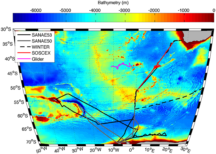
Figure 1. Trajectory of the Seaglider (SG573) between 20 September 2012 and 15 February 2013 (pink line) together with cruise tracks of SANAE 53 (black solid line), SANAE 50 (grey line), WINTER (black dashed line), and SOSCEx (red line) overlaid on the bathymetry of the study region.

The glider was programmed to profile between the surface and 1000 m continuously at a nominal vertical velocity of 10 cm s⁻¹. Each dive cycle (which includes a descent and ascent profile) took ~5 h to complete and covered an average horizontal distance of 2.8 km, rendering a temporal resolution of 2.5 h and a spatial resolution of 1.4 km (between each water column profile). Glider data were linearly interpolated to a 6-hourly frequency in order to grid unevenly spaced profiles, which typically ranged between 4 and 6 hourly. At the deployment and retrieval site of the glider, ship-based CTD cross-calibration casts were carried out yielding two independent inter-calibrations between the gliders, CTD sensors and bottle samples (Swart et al., 2015).

Glider fluorescence from a WETLabs ECO puck™ (BB2Fl-470/700) was dark corrected by subtracting the median fluorescence below 300 m from all raw instrument counts. Fluorescence quenching was isolated by selecting all daylight profiles between local sunrise and sunset plus 2.5 h (as quenching was on occasion observed in the profile following sunset). Fluorescence quenching was subsequently corrected using optical backscattering (b_bp), an alternate proxy for phytoplankton biomass that is not susceptible to quenching, based on the methods described in Sackmann et al. (2008). This method assumes a constant chlorophyll-to-carbon ratio throughout the surface waters and no cellular changes in chlorophyll packaging with depth as a photo adaptive strategy to low light levels. When backscattering was unavailable (intermittent sensor malfunction), quenching was corrected by extrapolating the maximum fluorescence value within the mixed layer to the surface according to Xing et al. (2012). In this method, the maximum fluorescence yield within the mixed layer is assumed to be representative of the mixed layer and implies homogeneity. This however is not necessarily the case as mixing and settling patterns between phytoplankton functional types are dynamic (Quéguiner, 2013). As such, when backscattering data are available, the Sackmann et al. (2008) method of quenching correction is preferred as it allows for small-scale variability in biomass with depth and reduces the possibility of overestimating surface chlorophyll values in the event of a subsurface chlorophyll maxima that is not biomass driven.

Fluorescence was converted to chlorophyll using a combination of the manufacturer's instrument specific chlorophyll conversion factor and in situ chlorophyll samples (250 ml filtered onto GF/F and extracted in 8 ml of 90% acetone for 24 h at −20°C) collected from CTD casts at glider intercept stations. This allowed all five gliders deployed during the SOSCEx experiment to be plotted simultaneously to form a statistically significant regression from 83 co-located glider chlorophyll and in situ chlorophyll samples (slope = 4.12, intercept = −0.21, r² = 0.66) with the manufacturer calibrated glider-based measurements being ~4 times higher than the ship-based chlorophyll measurements. The slope of the regression was applied to all glider chlorophyll data to correct the manufacturer conversion to chlorophyll to one more suited to the regional characteristics of Southern Ocean chlorophyll (see Swart et al., 2015 for more detail).

Spikes from raw backscattering (λ = 470) were separated using a 7-point running median filter according to Briggs et al. (2011). Raw digital counts were then converted into particulate backscattering (b_bp) according to Dall'Olmo et al. (2009), following the equation:

$\begin{array}{cc}\begin{array}{l}{b}_{bp470}=2\pi {\chi }_p\left[S(C-D)-{\beta }_{sw}\right]\hfill \end{array}& \left(1\right)\end{array}$

where S is the instrument specific scaling factor; C are the raw digital counts and D are the dark counts (factory value); χ_p (equal to 1.1) is the factor used to convert the particulate volume scattering function into b_bp (Boss and Pegau, 2001) and β_sw is the volume scattering of pure water estimated using the models of Zhang and Hu (2009) and Zhang et al. (2009). Remaining spikes in particulate backscattering were removed with a threshold in shallow (b_bp470 > 0.048) and deep (b_bp470 > 0.0025) water. Profiles with high mean backscattering (b_bp > 0.001) in deep waters (> 150 m) were identified as bad profiles and discarded (see Thomalla et al., 2015 for more detail).

Mixed layer depth (MLD) was defined following the criterion of de Boyer Montégut et al. (2004) as the depth where the difference in temperature exceeds 0.2°C in reference to the temperature at 10 m (ΔT_10m = 0.2°C). The temperature based criteria was chosen because (1) the salinity data (and hence density data) is contaminated in the final ~5 weeks of the glider data due to Gooseneck barnacles bio-fouling the conductivity cell of the CTD sensor and (2) intermittent spiking and thermal lag errors (see Garau et al., 2011) of the salinity data resulted in intermittent false MLD determinations when using a density criterion alone to determine the MLD. An investigation into the two MLD methods used on the glider data shows that they match each other closely (r = 0.86, p≪ 0.01) throughout the experiment (Swart et al., 2015).

Cruise Data

The in situ data used in this work were collected on four cruises to the Southern Ocean between austral winter 2012 and late summer 2013 (Table 1), which were typically separated into three legs: The GoodHope Line between Cape Town and Antarctica, the Buoy Run between Antarctica and South Georgia and the marginal ice zone along the continental margin (Figure 1). Data consisted of CTD casts and surface underway sampling for chlorophyll and POC collected routinely on SOCCO summer research cruises. CTD casts also provided b_bp470 data that were co-located with Niskin bottle samples for POC. Chlorophyll samples (250 ml) were filtered onto Whatmann 25 mm GF/F glass fiber filters and extracted in 8 ml of 90% acetone at −20°C for 12–24 h. Fluorescence was measured on a Turner Trilogy Laboratory Fluorometer and converted to chlorophyll using a standard chlorophyll dilution calibration. POC samples (~2 L) were filtered onto a pre-combusted 25 mm or 47 mm Whatmann GF/F filters and oven dried at 50°C. Filters were acidified by fuming with concentrated Hydrochloric Acid for 24 h to drive off inorganic carbon and re-dried in the oven. Filters were pelleted into 5 x 8 mm tin capsules and analyzed using a CHN analyser (Parsons et al., 1984; Knap et al., 1994). Blanks were interspersed every 6 to 20 samples (typically every 12). No replicate samples were analyzed.

TABLE 1

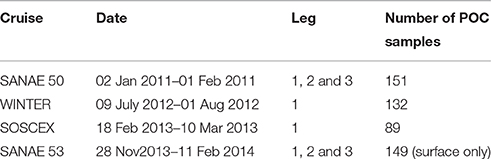
Table 1. Names and dates of the various cruises indicating the different legs covered and the number of POC samples per cruise, with leg 1 between Cape Town and Antarctica along the GoodHope Line, leg 2 from Antarctica to South Georgia and leg 3 along marginal ice zone (Figure 1).

Model Data

Numerical model results in the Sub-Antarctic zone were obtained from a simulation of the Biogeochemical Flux Model (BFM, http://bfm-community.eu) coupled with the NEMO ocean model (http://www.nemo-ocean.eu) at 0.25° resolution (PELAGOS025, McKiver et al., 2015). The BFM model (Vichi et al., 2007) allows computing phytoplankton dynamics in terms of stoichiometrically variable constituents, which also include variable chlorophyll to carbon ratios modified after Geider et al. (1997). All details of the model simulation are given in McKiver et al. (2015) and full descriptions of the biogeochemical model equations are available in Vichi et al. (2015). The variables extracted from the model results were total phytoplankton carbon and total phytoplankton chlorophyll, with the resulting dominant functional group in the region throughout the year being diatoms.

Estimation of Phytoplankton Carbon

Four different methods of deriving the fraction of phytoplankton-specific carbon (C_phyto) from backscattering and chlorophyll were applied to the glider optical data. They represent examples of the different types of methods available in the scientific literature.

Linear Method (30%POC)

Linear relationships between POC and backscattering were first proposed by Stramski et al. (1999). The high correlation in open ocean waters was the result of the dominant organic particle concentration which controls changes in both POC and b_bp (Stramski and Morel, 1990; Gardner et al., 1993; Stramski and Reynolds, 1993; Loisel and Morel, 1998). In this method 221 POC samples from the cruises listed in Table 1 (except SANAE53 where no CTD POC samples were available) were plotted against co-located b_bp470 data (Figure 2). POC and b_bp470 were linearly correlated with one another to provide a regression equation specific to the SAZ using a total least square method to account for the uncertainty in both the POC data and the backscattering:

$\begin{array}{cc}\begin{array}{l}POC=\left(39418\pm 3000\right)b_{bp470}-\left(13\pm 6\right).\hfill \end{array}& \left(2\right)\end{array}$

We have assumed an uncertainty of 7% for both the input data to the total least square regression and reported the slope with all digits, as it is customary in the literature (Table 2), with the addition of the standard error. The relationships between b_bp and POC from various ocean basins in the literature (Table 2) are included on Figure 2 for comparison.

TABLE 2

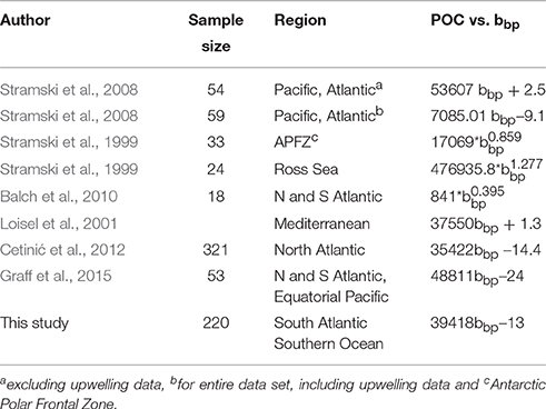
Table 2. Comparison of POC vs. b_bp reported from literature for original wavelength [taken from Cetinić et al. (2012)] with the addition of results from Graff et al. (2015) and this study.

FIGURE 2

Figure 2. Relationship between in situ POC and particulate backscattering (b_bp 470 nm) from cruise data (Table 1, SANAE53 was excluded as corresponding CTD backscattering data were not available) with the linear least squared regression (r² = 0.93) plotted in solid red. Overlain with fits (summarized in (Cetinić et al., 2012)) from (1) Stramski et al. (1999) from Ross Sea; (2) Stramski et al. (2008) from Atlantic/Pacific (excluding upwelling data); (3) Graff et al. (2015) from the North and South Atlantic and Equatorial Pacific; (4) Loisel et al. (2001) from Mediterranean; (5) Cetinić et al. (2012) from North Atlantic; (6) Stramski et al. (1999) from the Polar Frontal Zone (PFZ); (7) Balch et al. (2010) from north and south Atlantic; (8) Stramski et al. (2008) from Atlantic/Pacific (entire data set, including upwelling). See Table 2 for regression coefficients.

POC however still needs to be converted into a fraction specific to phytoplankton (C_phyto). Behrenfeld et al. (2005) summarized ranges of field based C_phyto:POC ratios from different oceanic regions to an average phytoplankton contribution to total POC of ~30%. Their 30% summary was derived from the studies of Eppley et al. (1992), Durand et al. (2001), Gundersen et al. (2001), and Oubelkheir (2001), where C_phyto:POC ratios ranged between 19 and 49% in regions that varied from eutrophic to oligotrophic. The 30%POC method as applied here converts b_bp470 into POC using the linear regression (Equation 2) and then uses a constant 30% fraction to represent C_phyto as the phytoplankton contribution to total POC. A comparison of glider b_bp470 with CTD b_bp470 from five collocated profiles (at glider deployment, intercept and retrieval sites) gave a slope of 0.99 (n = 104) making it possible to apply the regression from Equation (2) to the glider b_bp470 data to retrieve POC.

Behrenfeld et al. (2005) Method (B05)

Behrenfeld et al. (2005) derived a method of estimating C_phyto from remotely sensed backscattering data using a linear relationship between b_bp440 and chlorophyll. In this method, chlorophyll and b_bp at 440 nm (m⁻¹) were estimated using the Garver-Siegel-Maritorena (GSM) semi-analytical algorithm (Garver and Siegel, 1997; Maritorena et al., 2002; Siegel et al., 2002) applied to monthly SeaWiFS data from September 1997 to January 2002. While the b_bp wavelength analyzed by Behrenfeld et al. (2005) (440 nm) differs to our study (B05) (470 nm) this discrepancy would only result in a small percentage difference in b_bp values (Graff et al., 2015). As with Behrenfeld et al. (2005), our b_bp470 was corrected for contributions from non-algal organisms other than phytoplankton (which also contribute to the optical backscattering signal) by subtracting a background value of 3.5 10⁻⁴ m⁻¹, with the assumption that this value represents the portion of non-algal particulate matter that does not co-vary with phytoplankton (Behrenfeld et al., 2005). Worth noting however is that the proportion of non-algal particulate matter is not constant as was shown by a study in the Mediterranean where the non-algal contribution to particulate backscattering varied both seasonally and regionally by more than one order of magnitude (Bellacicco et al., 2016). Only 0.02% of the glider backscattering data fell below this threshold and they were discarded. The corrected b_bp470 was then converted into C_phyto through the equation

$\begin{array}{cc}\begin{array}{l}{C}_{phyto}=13000\left(b_{bp470}-3.5 {10}^{-4}\right).\hfill \end{array}& \left(3\right)\end{array}$

The slope was chosen by Behrenfeld et al. (2005) to give satellite chl-a:C_phyto values within the range compiled by Behrenfeld et al. (2002) from laboratory experiments (average = 0.010, range = 0.001 to >0.06) and to give an average phytoplankton carbon contribution to total particulate organic carbon of ~30% (range: 24 to 37%). Behrenfeld et al. (2005) did not provide any statistical assessment of the estimated parameters.

Martinez-Vicente et al. (2013) Method (M13)

Martinez-Vicente et al. (2013) derived phytoplankton carbon from the relationship between C_phyto and in situ backscattering b_bp470 from the euphotic zone of a latitudinal study of the Atlantic ocean using a total least square linear regression. C_phyto was directly estimated from flow cytometry for 6 different groups of phytoplankton using information on phytoplankton abundances, cellular carbon per unit volume and mean cell volume. The total C_phyto concentration per sample was calculated as the sum of the contributions from each phytoplankton type. A significant linear relationship was found between b_bp470 and C_phyto:

$\begin{array}{cc}\begin{array}{l}{C}_{phyto}=\left(30100\pm 1100\right)\left[b_{bp470}-\left(7.6\pm 0.4\right) {10}^{-4}\right]\hfill \end{array}& \left(4\right)\end{array}$

The linear regression was limited to b_bp470 < 0.003 m⁻¹ because samples above this threshold value (n = 8) exhibited a shift in the relationship that was not possible to describe with a single linear function. In this study we applied the M13 Equation (4) to all glider data, even those higher than 0.003 m⁻¹ (these are all surface data representing about 3% of the total, with values up to 0.0048 m⁻¹). In addition, the form of Equation (4) implies that the domain does not comprise b_bp values lower than 7.6 10⁻⁴ m⁻¹. Since in this study most of the b_bp470 values collected by the glider sensor deeper than 150 m were lower than this threshold (about 54% of the total data), they were discarded from the analysis during the application of the method.

Sathyendranath et al. (2009) Method (S09)

Sathyendranath et al. (2009) derived a method of estimating C_phyto using chlorophyll and POC observations from offshore regions of the North West Atlantic Ocean and the Arabian Sea. In their study, the authors considered that POC incorporates all types of particulate carbon in the system (including phytoplankton, bacteria, detritus, and viruses). The S09 method then assumes that for any given chlorophyll concentration, the minimum particulate carbon content represents an upper bound on phytoplankton carbon. In the S09 method, the authors log-transformed both POC and chlorophyll to linearize the relationship and to reduce the weight of the stations with high values of POC and chlorophyll in the regression analysis. They then used a 1% quantile regression to represent the upper limit on carbon content from phytoplankton alone.

This method can be applied to the available data from the South Atlantic Southern Ocean, using co-located POC and chlorophyll data from both underway and profile CTD samples collected on all cruises listed in Table 1 and depicted in Figure 1. The 1% quantile regression was fitted to the log- transformed data (Figure 3) to derive the following equation:

$\begin{array}{cc}\begin{array}{l}{C}_{phyto}=42 {(chl)}^{0.86}\hfill \end{array}& \left(5\right)\end{array}$

The relationships derived by Buck et al. (1996) and Sathyendranath et al. (2009) are included in Figure 3 for comparison and show that the SAZ data are characterized by lower carbon content per unit chlorophyll and that the values converge to the Sathyendranath et al. (2009) line at higher chlorophyll concentrations (Figure 3).

FIGURE 3

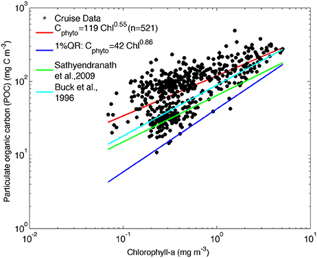
Figure 3. POC against chlorophyll for all cruise data. The least-square fit to log-transformed data is shown in red [log₁₀ POC = (2.08 +/− 0.01) + (0.55 +/− 0.03) log₁₀ Chla], the C_phyto minimum carbon estimates by quantile regression [log₁₀ POC = (1.63 +/− 0.05) + (0.86 +/− 0.09) log₁₀ Chla, p = 0.01], in dark blue. The relationship between phytoplankton carbon and chlorophyll from Sathyendranath et al. (2009) (green line) and Buck et al. (1996) (light blue) are shown for comparison.

Results

Seasonal Evolution of Chlorophyll and POC

The glider transect showed substantial seasonal changes in chlorophyll (Figure 4A) with relatively low chlorophyll concentrations (<0.5 mg m⁻³) found at the beginning of the transect between late September and October, coinciding with the deepest MLDs (down to 200 m). Periods of enhanced chlorophyll were shown to be associated with submesoscale physical forcing of the MLD by Swart et al. (2015) and Thomalla et al. (2015). The spatial scales of the physical field are evident in Supplementary Figure 1, and investigated in more detail in a study by Du Plessis et al. (in review; see also their Figure 6), which shows small-scale excursions of mixed layer density and surface (100 m) stratification for the glider time series. These rapid changes in density are associated with submesoscale features that actively slump horizontal density gradients (Mahadevan et al., 2012) driving enhanced stratification during periods of lighter mixed layers and weaker stratification when mixed layers are dense (Supplementary Figure 1) (Du Plessis et al., in review). The shoaling of the MLD from ~100 to 20 m through seasonal heat flux in late November saw a concomitant increase in surface chlorophyll (>0.55 mg m⁻³) that was sustained throughout summer until the end of the sampling period in mid-February.

FIGURE 4

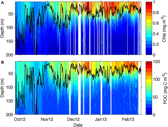
Figure 4. Section plot from the glider transect data for (A) chlorophyll and (B) particulate organic carbon (POC) derived from backscattering data from equation (2). The mixed layer depth is marked as a solid black line.

Overall, there is a rather good visual correspondence between the seasonal evolution of chlorophyll and POC (Figure 4B), which was attained through the application of equation 2 to the glider b_bp470 data. The bulk of POC was located within the MLD, as it occurs for chlorophyll, with lowest POC concentrations (50–80 mg C m⁻³) being observed in October, increasing in November (to about 80–120 mg C m⁻³) and reaching maximum concentrations in December (with values up to 150 mg C m⁻³) extending through to February. The more evident difference between the datasets is in late October where an increase in POC is not observed in chlorophyll and in early January, when a decrease in POC is not observed in chlorophyll.

Phytoplankton Carbon Estimates

Figures 5B–D compares the results from the different C_phyto methods for selected depths. Corresponding chlorophyll concentrations are also shown (Figure 5A). C_phyto shows a very similar seasonal distribution to that of chlorophyll and very little difference between surface 10 and 40 m concentrations highlighting the homogeneity expected in well-mixed surface waters. When applied to the glider b_bp470 and chlorophyll data, 3 of the methods of retrieving C_phyto described in Section Discussion showed similar results, despite differences in the equations used. The 30%POC and B05 methods (Figures 5B–D) showed almost identical distribution patterns with concentrations ranging between 0 and 45 mg C m⁻³. This is not surprising since the slope of the B05 equation is about 1/3 of the one found in Equation (2), and by assuming a 30% contribution due to phytoplankton carbon the numbers become similar. These slopes are also very similar to the more recent equation developed by Graff et al. (2015) C_phyto = 12128(b_bp470 + 4.86 x 10⁻⁵) (their Figure 3) that utilized direct measurements of C_phyto from the temperate South Atlantic, equatorial upwelling and oligotrophic gyres. In addition, the S09 method (Figure 5D), the only method that uses chlorophyll rather than particulate backscattering to retrieve C_phyto, showed remarkably similar results to the methods of B05 and 30%POC.

FIGURE 5

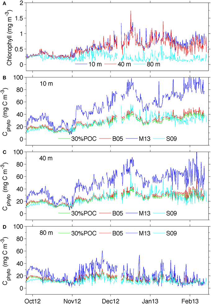
Figure 5. (A) Temporal chlorophyll distribution at different depths and (B) temporal distribution of phytoplankton carbon at 10 m, (C) 40 m and (D) 80 m See supplementary Figure 3 for a version of panel (B) showing the ranges derived from using the standard error of the estimates for 30%POC equation (2), M13 equation (4), and S09 equation (5).

Values of C_phyto from the M13 method were overall much larger, particularly at 10 and 40 m (Figures 5B,C), with values up to 80 mg C m⁻³. With this method, surface concentrations of C_phyto in October (~30–40 mg C m⁻³) were lower relative to the remaining transect but high when compared to the other three methods (~20 mg C m⁻³). Similarly, from November to February, high surface C_phyto from M13 ranged from ~40–100 mg C m⁻³ compared with ~ 20–50 mg C mg⁻³ in the other three methods. The discrepancy between M13 and the other methods decreases with depth (80 m) and is less prominent at the beginning of the transect (October). This indicates that the difference between M13 and the other three methods is generally smaller when chlorophyll concentrations are low (<0.5 mg chl-a m⁻³) in early spring and at depth (>80 m).

Seasonal Changes in Chlorophyll to Phytoplankton Carbon Ratios

In general, the surface ratios (Figure 6) appear lower in October (0.01–0.02) when mixed layers were deeper and chlorophyll concentrations were low, increasing toward mid-January (0.02–0.04) with decreasing mixed layers and increasing concentrations of phytoplankton biomass (Figure 4). The S09 method, despite being less variable through its dependence on chlorophyll alone, shows a similar background value to the chl-a:C_phyto ratios of the B05 and 30%POC methods, except at the beginning of the time series (last week of September through to the first week of October) where a decrease in chlorophyll is not mirrored by a corresponding decrease in C_phyto (from b_bp470 computed methods) resulting in low chl-a:C_phyto ratios (from b_bp470 computed methods). A similar deviation occurred in the last week of January to the first week of February where S09 chl-a:C_phyto ratios were noticeably higher than B05 and 30%POC but this time due to an increase in C_phyto (from b_bp470 computed methods) that was not evidenced in chlorophyll. A final example of where chl-a:C_phyto ratios between fluorescence based and b_bp470 based methods deviated is in the last week of October where a peak in the chl-a:C_phyto ratios from b_bp470 computed methods (Figure 6) was the result of a distinct drop in carbon that was not evident in chlorophyll (see also Figure 4B).

FIGURE 6

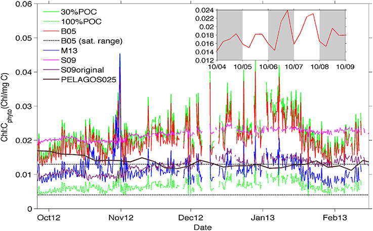
Figure 6. Time-evolution of chl-a:C_phyto ratios at the surface (10 m) derived from the 30%POC method (solid lighter green top line), the B05 method (red line), the M13 method (blue line), and the S09 method (pink line). In addition, Chl-a:C_phyto ratios were calculated using the chl-a:POC ratio from the cruise data (which implies that all POC is phytoplankton specific) and is presented as 100%POC (darker green bottom dashed line). Included for comparision are (1) the chl-a:C_phyto ratios derived from the original equation from Sathyendranath et al. (2009) presented as S09original (purple line), (2) the satellite range of ratios from Behrenfeld et al. (2005) (black dotted lines) and (3) the ratios derived from the PELAGOS025 model (McKiver et al., 2015, extracted from the model for the same geographical co-ordinates as the glider transect in time but for a year 2011 simulation, solid black line). The inset shows a detail of the daily signal for the B05 method.

The ratio obtained with the M13 method is about half that obtained from the other methods, with similar short term time variations (~1–7 days) to the other b_bp470 derived methods but a different seasonal time evolution (i.e., no tendency for M13 chl-a:C_phyto ratios to increase from October to mid-January). The seasonal evolution of low to high chl-a:C_phyto ratios from spring to summer is evidenced in 30%POC, B05 and S09 methods.

The ratios obtained from the glider data in the SAZ are usually larger than the range obtained with global satellite data (Behrenfeld et al., 2005) as shown in Figure 6. This range is more in agreement with the M13 method and the ratio obtained by applying the original Sathyendranath et al. (2009) equation to the data, or by considering all POC as phytoplankton carbon. Interestingly, the model simulation by McKiver et al. (2015), which parameterizes a dynamical ratio, also shows a similar value even if the temporal trend is opposite.

Discussion

This study uses a high-resolution glider data set from the sub-Antarctic Southern Ocean to compute C_phyto using four different methods available in the literature. The ability to get sound estimates of C_phyto is important as it provides a measure of phytoplankton carbon biomass that is core to many models of net primary productivity, a key indicator of the carbon cycle. In addition, good measurements of C_phyto enable us to better understand changes in cellular chlorophyll-to-carbon ratios, which provides information on phytoplankton physiology (e.g., cellular adjustments to changes in light, temperature, and nutrients, Behrenfeld et al., 2005). As such, deriving good estimates of C_phyto and chl-a:C_phyto ratios will enable us to refine model parameterizations of phytoplankton dynamics (Sathyendranath et al., 2009). Since the biological pump in the Southern Ocean drives 33% of global organic carbon flux (Schlitzer, 2002; Lenton et al., 2013), it is of particular importance that we improve our understanding of the biological response of Southern Ocean phytoplankton to climate change.

Comparison of the Methods

Rather than assess the quality and merit of individual methods of deriving C_phyto against each other, which would require independent phytoplankton data that would inevitably be limited in time and space, this study aims to evaluate the differences of the various methods using high frequency optical glider data from the SAZ as a benchmark. It should also be noted that the methods applied in this research were developed using different data obtained from different oceanic regions. The M13 method is the only equation that was derived from in situ C_phyto data (computed from cell counts and assumptions of carbon content per cell) but from a latitudinal study of the Atlantic; the B05 equation is also non-specific to the Southern Ocean and derived from global satellite data; the 30%POC and S09 methods were recomputed using in situ POC and chlorophyll data from the Southern Ocean. To further extend the number of methods, the original equation from the S09 method developed using data from the NW Atlantic and Arabian Sea (Sathyendranath et al., 2009) has been included in Figures 6, 8 for comparison (presented as S09original).

The most evident result of the comparison is that three of the methods cluster together (30%POC, B05, and S09) with only one (M13) being substantially different in magnitude from the others (Figure 5). Despite their different origins, C_phyto from 30%POC, B05, and S09 (the only method that is derived from chlorophyll) all show similar results. The similarity in C_phyto derived using B05 (which made use of a global data set to convert b_bp to POC) and 30%POC (that used a regionally specific conversion based on Southern Ocean filtered samples) implies that the conversion from b_bp to POC used here is regionally robust. This is confirmed by a comparison of the POC vs. b_bp relationship from previously published values (Figure 2, Table 2), which shows the slope of the regression between POC and b_bp to fall well within the observed literature range from various ocean basins. The relationship from our data (from the south Atlantic Southern Ocean; Figure 2, Table 2) is very similar to that generated from the Mediterranean (Loisel et al., 2001), the North Atlantic Bloom Experiment (NABE, Cetinić et al., 2012) and the Polar Frontal Zone (PFZ, Stramski et al., 1999). Our POC vs. b_bp slope is however lower than that from the North and South Atlantic and Equatorial Pacific (Graff et al., 2015), the Ross Sea (Stramski et al., 1999), and the slope that is the basis of the NASA POC algorithm (Stramski et al., 2008), using data from the Pacific and Atlantic but excluding data from the upwelling regions (Cetinić et al., 2012). On the contrary, our slope is higher than that from the Atlantic and Pacific including data from the upwelling regions (Stramski et al., 2008) and yields higher POC (for b_bp >0.0027) when compared to the relationship from the north and south Atlantic (Balch et al., 2010).

The M13 method returns much higher concentrations of C_phyto with the difference being less when chlorophyll concentrations are below < 0.5 mg m⁻³) in the month of October (Figure 5) and at depth (~ 80 m). The reason for the higher C_phyto estimates using M13 is the steep slope (30100) of Equation (4), which is more than twice the slopes used in B05 (13000) and 30%POC (11825). The comparatively steep slope of M13 was noted in Martinez-Vicente et al. (2013) and the explanation proposed for the doubling of parameters between their equation and that of Behrenfeld et al. (2005) was due to “uncertainties in satellite and in situ estimates of b_bp and/or differences in the spatio-temporal scales of the two studies.” A big difference in the steepness of the slope was similarly noted between M13 (slope = 30100) and a study by Graff et al. (2015) in the North and South Atlantic and Equatorial Pacific (slope = 12128). They suggest that the difference may be due to variability in the assumed volume-based phytoplankton biomass conversions used in the M13 method to convert volume to C_phyto. This can yield an order of magnitude variability in resultant C_phyto estimates (Caron et al., 1995; Dall'Olmo et al., 2011).

Equation (4) from Martinez-Vicente et al. (2013) was generated from the typically low biomass region of the Atlantic, where in situ b_bp data were generally less than 0.003 m⁻¹. The eight data points that exceeded this threshold were removed from the regression by the authors, as they showed a shift in the relationship that could not be described with a single linear function. An inclusion of the 8 data points (where b_bp was > 0.003) would drive an even steeper slope, even higher concentrations of C_phyto, and a greater disagreement between the different methods used here. These 8 data points were characteristic of eutrophic conditions (as opposed to oligotrophic conditions) where larger cells characterized the phytoplankton community (more Nano- and Pico- eukaryotes and less Prochlorochoccus) with lower b_bp:C_phyto ratios (see Martinez-Vicente et al., 2013, their Supplementary Figure 1). Similarly, if microphytoplankton were included in their measurements (missed by flowcytometry), the slope would likely be even steeper. This would be consistent with optical theory that predicts a decrease in b_bp:C_phyto ratios with an increase in particle size, where C_phyto is proportional to volume (Boss et al., 2004; Martinez-Vicente et al., 2013). However, worth noting is that this theory represents phytoplankton cells as homogenous spheres that can overestimate the real refractive index for certain species (Vaillancourt et al., 2003). As described in Section Martinez-Vicente et al. (2013) method (M13), the M13 equation was applied to all glider b_bp data (ranging from 0.001 to 0.01 m⁻¹), with much of the data falling above the domain of applicability of Equation (4) (b_bp <0.003). It is thus possible that the overestimated C_phyto concentrations generated from the M13 method are the result of an unsuitable application of a regionally derived model from the low backscattering field of the Atlantic to the relatively high backscattering SAZ. This possibility is supported by all four methods generating similar C_phyto concentrations when biomass was below 0.5 mg m⁻³ (i.e., in early spring and at depth ~ 80 m, Figure 5). As such, when chlorophyll concentrations are below 0.5 mg m⁻³ it appears to make little difference which method of estimating C_phyto is chosen by the user.

The S09 method showed similar C_phyto results in range and distribution to both B09 and 30%POC, highlighting its robustness in converting chlorophyll to C_phyto. This information is particularly useful for data sets that require conversion to phytoplankton specific carbon in the absence of backscattering measurements. However, when the chl-a:C_phyto ratios from the different methods are compared (Figure 6), the limitations of the S09 method are highlighted, namely the very low temporal variability in chl-a:C_phyto ratios. This can be attributed to the derivation of chl-a:C_phyto ratios from a monotonic function of chlorophyll concentration:

$\begin{array}{cc}\begin{array}{l}chla:C_{phyto}=\frac{1}{a} {(chla)}^{1-b}\hfill \end{array}& \left(6\right)\end{array}$

where a = 42 and b = 0.86 are the coefficients derived from Equation (5). The implication of this is that the S09 method, though being non-linear, does not allow for a scenario where C_phyto increases or decreases without a corresponding change in chlorophyll. The remaining three methods on the other hand allow C_phyto to vary independently of chlorophyll, which accounts for the higher temporal variability observed in the chl-a:C_phyto ratios using the B05, 30%POC and M13 methods (Figure 6).

Seasonal and Sub-Seasonal Variations in the Chlorophyll-to-Carbon Ratio

How do surface chlorophyll-to-carbon ratios (chl-a:C_phyto) vary in time? In general chl-a:C_phyto ratios tend to be lower in spring (October), higher in summer (December – January), and decreasing again in late summer (February) in particular in the backscattering methods (30%POC, B05, and M15). The absence of a strong seasonal evolution in M13 is likely a consequence of the method which drives higher C_phyto (relative to the other methods) when chlorophyll concentrations are high, and more similar C_phyto when chlorophyll is below 0.5 mg m⁻³ thus dampening any seasonal driven signal in surface chl-a:C_phyto ratios.

According to the literature, chl-a:C_phyto ratios tend to be highest when larger diatoms are present and lowest when smaller species dominate (e.g., Prochlorococcus) (Sathyendranath et al., 2009). As such, some of the seasonal variability observed in the chl-a:C_phyto ratios could be the result of different sized species dominating the community at different times. Smaller cells in spring (October) when light is potentially limiting (mean MLD = 87 m and mean PAR in MLD = 0.01 μ E cm⁻² s⁻¹) and late summer (January) when nutrients are potentially limiting (depleted reservoir), vs. larger cells in early summer (December) when light (Supplementary Figure 2) and nutrients are thought to be unrestricted (mean PAR in MLD = 0.03 μ E cm⁻² s⁻¹). Previous studies have shown that the range of chl-a:C_phyto ratios observed in the Southern Ocean are the result of seasonal variation in the physiological response of phytoplankton to light and nutrient limitation (Behrenfeld et al., 2005). Phytoplankton chl-a:C_phyto ratios tend to decrease with increasing light conditions and decreasing temperature and nutrient concentrations (and vice versa) (Geider et al., 1997; Socal et al., 1997; Taylor et al., 1997; Behrenfeld et al., 2005; Lü et al., 2009; Halsey and Jones, 2015; Westberry et al., 2016). Increasing chl-a:C_phyto ratios as a physiological response of phytoplankton to low light conditions enables them to increase their light harvesting ability by increasing the volume of chlorophyll packed into their cells (Behrenfeld and Milligan, 2013; Halsey and Jones, 2015; Bellacicco et al., 2016). Indeed, photoacclimation to changes in the underwater light field as a bloom develops have been known to account for the entire range of seasonal variability observed in bulk chlorophyll (e.g., Winn et al., 1995; Westberry et al., 2008). However, since Fe reservoirs are replenished in winter through deep mixing and depleted through biological uptake in the Spring Summer growing season (Boyd et al., 2010), nutrients are not considered the likely driver of the observed increase in chl-a:C_phyto ratios. Similarly, both light (through increased PAR Supplementary Figure 2 and decreased MLD Figure 4) and temperature (see Thomalla et al., 2015 their Figure 2B) tend to increase from October to December. It is thus unlikely that these processes (light, temperature or nutrients) are responsible for the seasonal increase in chl-a:C_phyto ratios observed during this period (Figure 6). However, since laboratory studies consistently show a decrease in chl-a:C_phyto ratios under Fe stress (Greene et al., 1992; Sunda and Huntsman, 1995), it is possible that limiting nutrients could contribute to the observed decrease in chl-a:C_phyto ratios in late summer (February). Similar results of declining chl-a:C_phyto ratios were observed by Behrenfeld et al. (2005) in regions dominated by large spring–summer blooms in phytoplankton abundance, where a decrease in chl-a:C_phyto ratio was observed prior to the seasonal biomass crash.

The physiological response of phytoplankton to relief from Fe stress has shown increases in chl-a:C_phyto ratios as growth rate increases (Greene et al., 1992; Geider et al., 1997; Sunda and Huntsman, 1997). This response is the result of upregulation of photosynthetic machinery and light harvesting capacity (Laws and Bannister, 1980). A measure of the growth rate estimated as the rate of change of MLD integrated chlorophyll (Supplementary Figure 2) shows an increase from 0 at the beginning of the time series (October) to ~0.017 mg chl-a m⁻² d⁻¹ in mid-December. Although we are unable to quantify the role of Fe in this study, the increase in chl-a:C_phyto ratios over the same time period may be a physiological response to increased growth rates when neither Fe or light were considered limiting. This was a similar response to what was observed during bloom conditions by Westberry et al. (2013) in both natural and purposeful Fe addition experiments. In addition, phytoplankton must photoacclimate as the bloom develops to counter the effects of self-shading, further increasing chl-a:C_phyto ratios over the growing season.

Finally, an alternative explanation for the observed seasonal increase in chl-a:C_phyto ratios is that the ratio of C_phyto to total POC (and to b_bp) decreases as the seasonal bloom develops. In other words, as the season progresses a greater percentage of the particulate backscattering signal is due to non-phytoplankton specific carbon (e.g., heterotrophic bacteria, detritus, viruses, ciliates) (Christaki et al., 2011). This was observed in a study in the Mediterranean where the non-algal contribution to b_bp470 was generally larger in the more productive regions that had elevated phytoplankton abundances (Bellacicco et al., 2016). Behrenfeld et al. (2005) reported that a compiled data set of field derived C_phyto:POC ratios spanning oligotrophic to eutrophic ocean regions ranged from 19 to 49%. These differences reflect system variability in producer-consumer dynamics, processes influencing the particle field and possible differences in export efficiency (Graff et al., 2015). If this ratio varies seasonally as much as regionally (i.e., by a factor of 2.5), it will have a substantial effect on optically derived chl-a:C_phyto ratios. Of the four methods applied here, all three b_bp470 computed methods (B09, 30%POC and M15) apply a constant C_phyto:POC ratio with time. On the other hand, the S09 method may indirectly account for adjustments in C_phyto:POC through the non-linear relationship between chlorophyll and C_phyto that drives an increase in chl-a:C_phyto ratios with increasing chlorophyll. To elaborate; as the bloom develops, phytoplankton biomass increases with a concomitant decrease in the percentage of C_phyto relative to total POC. This may be reflected in the logarithmic relationship between chlorophyll and C_phyto (Figure 3), which would be observed as an increase in chl-a:C_phyto ratios with increasing chlorophyll concentrations in the S09 method (Figure 6).

Over and above the characteristic seasonal cycle in chl-a:C_phyto ratios, there is strong sub-seasonal and daily variability that are likely driven by phytoplankton community responses to smaller scale physical processes and day-night physiological adjustments. In the case of the M13 method, where the seasonal cycle is dampened, one can argue that the smaller sub-seasonal scales are in fact dominating the variability. Some distinct examples of smaller scale adjustments in the chl-a:C_phyto ratios are as follows:

1. The low chl-a:C_phyto ratios (from b_bp470 derived methods) at the very beginning of the time series (late September/early October) (Figure 6) that are associated with deep MLD's (~150 m, Figure 4) when the glider crosses the cold core of a mesoscale cyclone ~200 km in diameter (Swart et al., 2015);

2. A peak in chl-a:C_phyto ratios (from b_bp470 derived methods) in the last week of October (Figure 6) that coincides with an intense shoaling of the MLD to ~25 m (Figure 4), the timescale of which relates to an oceanographic feature and an event that is mesoscale in nature (slumping of the lateral gradient in density) (Mahadevan et al., 2012; Swart et al., 2015); and

3. A distinct daily signal in chl-a:C_phyto ratios with higher ratios during the day that are arguably the result of daily physiological adjustments in phytoplankton chlorophyll content per unit carbon.

The drivers of sub-seasonal variability in chl-a:C_phyto ratios seen in late September (low) and late October (peak) are clearly linked to mesoscale features and associated adjustments in the depth of the mixed layer, which is deep in late September (~150 m) and shallow in late October (~25 m). However, the adjustments in chl-a:C_phyto ratios are not a physiological response of the phytoplankton to light. Were this the case, the opposite response would be true i.e., an increase in chl-a:C_phyto ratios would be observed when MLD's were deep and light was supposedly limiting. It is thus more likely that these small scale adjustments in chl-a:C_phyto ratios are the result of a shift in community structure from a small cell dominated community with low growth rates in late September to a population dominated by large cells with high growth rates under high light conditions in late October.

To test whether the diurnal variability in the chl-a:C_phyto signal (see insert in Figure 6) was driven by an artifact of residual uncorrected solar quenching (or the quenching correction itself), we compared in Figure 7 the linear regressions of midnight and midday C_phyto (r² = 0.93) to midnight and midday chlorophyll (r² = 0.66). Although the coefficient of determination for chlorophyll is lower, this is what can be expected from the effects of acclimation. The normal dispersion of the data however suggests that the variability in chlorophyll is not biased and hence implies that there is no systematic artificial error introduced through the quenching correction (Figure 7). As such, it is believed that the daily signal in chl-a:C_phyto ratios is a real response of the phytoplankton community. Interpreting this diurnal variability is difficult as it depends on numerous parameters that include phytoplankton concentration, composition and physiological status together with the detrital and small heterotroph concentration, all of which are typically not known and hence diurnal variability in chl-a:C_phyto ratios remains poorly understood. The likely drivers however include the balance between daytime production and night time degradation, changes in particle size distribution and changes in the refractive index driven by varying internal concentrations of organic compounds (e.g., accumulation of intracellular carbon through photosynthesis) (Kheireddine and Antoine, 2014). Although this small-scale variability elicits further detailed investigations it remains outside of the scope of this manuscript.

FIGURE 7

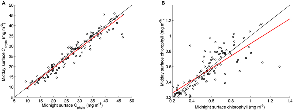
Figure 7. Linear regressions of daily surface midnight vs. daily surface midday concentrations of (A) C_phyto from the glider transect using the B05 method (slope = 0.97, r² = 0.93, rmse = 2.49) and (B) chlorophyll (slope = 0.8, r² = 0.66, rmse = 0.15). The linear least square regression line appears in red with the one to one line in black.

Implications for Model Parameterizations

Some biogeochemical models apply a constant chl-a:C_phyto ratio globally (usually 0.02 mg chl-a mg C⁻¹) even if the constraints are not developed equally (i.e., some regions are data poor), while others have a dynamical function that should include acclimation to prevailing light conditions. It is entirely possible that the inadequate parameterization of this ratio is the reason for the seasonal biases found in biogeochemical models (Doney et al., 2009; Steinacher et al., 2009; Vichi and Masina, 2009). In Figure 6 we compare the chl-a:C_phyto ratios generated from a Southern Ocean data set (using the different optical methods) with those constrained in satellite data, cruise data and from one medium resolution global model (the PELAGOS025 model analyzed by (McKiver et al., 2015), Model data). The chl-a:C_phyto data from the model was extracted from the same location as the glider transect and over the same dates (month and day) but from a simulation for the year 2011, due to a limitation in the availability of atmospheric forcing functions.

Since C_phyto cannot exceed POC, the chl-a:POC ratio from the cruise data (Table 1) was used to set a minimum chl-a:C_phyto ratio assuming all POC was phytoplankton specific (presented as 100%POC, Figure 6). These ratios were understandably low (<0.01 mg chl-a mg C⁻¹) but above the minimum satellite range (0.004 mg chl-a mg C⁻¹) of Behrenfeld et al. (2005) and oftentimes close in magnitude to the ratios generated by the M15 method. The ~50% lower chl-a:C_phyto ratios for M13 are driven by the high C_phyto values that this method generates relative to the other methods, particularly when biomass is high (December to February). It was proposed earlier that the low chl-a:C_phyto ratios were a possible result of an unsuitable application of a regionally derived model from the Atlantic to the SAZ. The S09 method allows us to do a direct comparison of the chl-a:C_phyto results generated from one model derived predominantly from data from the NW Atlantic (S09original) with the same model but derived from data from the Southern Ocean (S09, Figure 6). This comparison shows how the application of the S09original model to the SAZ data set results in much lower chl-a:C_phyto ratios that are more inline with those generated by the M13 method, that was similarly derived from cell counts from the Atlantic.

Both the M13 and S09original methods produce chl-a:C_phyto ratios that are very similar to the 100%POC method, which outputs the minimum ratios possible assuming all POC is phytoplankton specific. This is not surprising when one considers that the slope of the M13 method (30100 mg C m⁻²) is 76% of the POC: b_bp slope found in this study (39418 mg C m⁻²) (Figure 2). This finding implies that when the M13 method is applied to the glider data set, there is very little non-algal POC that co-varies with C_phyto. This result is unlikely if one considers that the maximum C_phyto:POC ratio reported by Behrenfeld et al. (2005) is 49% and in the Equatorial Upwelling and temperate spring waters of the Graff et al. (2015) study rarely exceeded 40% (mean = 25%). Although phytoplankton has been known to dominate POC at a high biomass coastal upwelling site (Hobson et al., 1973) this observation is in contrast to the typical low contribution of C_phyto to POC in productive offshore waters (Hobson et al., 1973; Andersson and Rudehäll, 1993). As such, it is more likely that the slope of the M13 method (and S09original) is too high for this region and that the 30%POC, S09 and B05 methods are more appropriately applied to Southern Ocean data sets, supporting the argument of an unsuitable application of a regionally derived model from the Atlantic to the SAZ. The M13 method still resolves the shorter-term variations likely driven by photo-physiology but reduces the summer increase in the ratio explained by adjustments in nutrient driven growth rates and community structure.

A comparison of the results with the PELAGOS model (Figure 6) imply that an overall chl-a:C_phyto ratio of 0.02 mg chl-a mg C⁻¹ seems adequate to represent the SAZ phytoplankton during spring and summer. However, the glider data indicate that the sub-seasonal and seasonal variations of this parameter are rather high and may play an important role in determining the magnitude of the bloom. In addition, the PELAGOS025 model shows an apparent misrepresentation of the seasonal cycle of chl-a:C_phyto ratios, with high ratios in winter and low ratios in summer (whereas the glider shows an increase in the chl-a:C_phyto ratios from winter through to summer). This is likely because PELAGOS025 is based on the Biogeochemical Flux Model (Vichi et al., 2007; Vichi and Masina, 2009) that uses a variation of the Geider et al. (1997) formulation for light acclimation and chlorophyll regulation. As such, the seasonal mismatch may be a result of the model assumption that all seasonal variability is purely due to acclimation to a prescribed high optimal chl-a:C_phyto ratio (deep mixed layers in winter driving increased chlorophyll synthesis through packaging responses to low light conditions). This may explain the observed seasonal biases of the models when compared with ocean color data reported in the literature. Rather, if our estimates of C_phyto based on backscattering are appropriate for the Southern Ocean (and this can only be validated with corresponding in situ estimates) then the glider data suggest that models need to account for low light adaptation in winter, which would dampen the acclimation response and allow for lower optimal chl-a:C_phyto ratios in winter. While in summer, the large increase in chlorophyll may need to coincide with a shift toward a community characterized by larger cells, relatively higher growth rates and higher optimal chl-a:C_phyto ratios. Such a mechanism is currently not implemented in any of the biogeochemical models because they usually consider one single group of diatoms. Numerical models, even the ones with a more sophisticated physiology like the BFM (or PISCES) may account for acclimation to light but are still dominated by the same kind of diatoms without any additional plasticity. The PELAGOS025 model does however do a better job in capturing the range of observed chl-a:C_phyto ratios, which the satellite data do not (Figure 6; see satellite range from Behrenfeld et al. (2005) for the Southern Ocean 0.004 – 0.013, their Table 1).

A Reference Chlorophyll-to-Carbon Ratio for the Sub-Antarctic Zone?

The data used for this research provides for the first time Cphyto obtained from a high-resolution glider data set to derive independent surface chl-a:Cphyto ratios from the SAZ. This is a much-needed parameter for biogeochemical models to improve the simulation of phytoplankton blooms in the region. To summarize the range of results obtained with the glider data from the different methods described in Section Materials and Methods, we compare in Figure 8 their surface (10 m) chl-a:Cphyto ratios to several literature values and ranges (Montagnes et al., 1994; Sunda and Huntsman, 1995; Llewellyn and Gibb, 2000), as well as to the model results, using non-parametric distributions (mean, median and 5–25 percentiles).

FIGURE 8

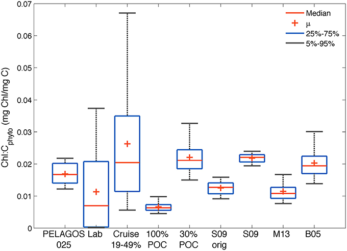
Figure 8. Comparison of the distribution of chl-a:Cphyto ratios derived from (1) the four glider estimates in the SAZ (30%POC, S09, M13 and B05); (2) the PELAGOS025 model for the glider transect (0–10 m); (3) a collation of laboratory culture experiments from the literature [Lab: n = 127, Supplementary Table 1 (Montagnes et al., 1994; Sunda and Huntsman, 1995; Llewellyn and Gibb, 2000)]; (4) from Southern Ocean cruise data (Cruise, 0–20 m) assuming a phytoplankton carbon fraction of 19, 30, and 49%; (5) minimum possible ratios derived from the glider data if all POC was phytoplankton specific (100%POC) and 6) from the original Sathyendranath et al. (2009) model developed from data from the NW Atlantic and Arabian Sea (S09orig).

Our analysis suggests that it is not possible to establish one single value for the conversion between chlorophyll and carbon. The large range of observed variability is driven by methodological uncertainties, regional differences and large seasonal variations. All chl-a:C_phyto ratios from the different methods applied to the glider data set (30%POC, B05, S09, M15) fell within the data set limits compiled by Behrenfeld et al. (2002), which for the global ocean range between 0.001 and >0.06 mg chl-a mg C⁻¹ (Behrenfeld et al., 2005). Similarly, all methods generated chl-a:C_phyto ratios that fell within the range of laboratory culture measurements collated here (Supplementary Table 1) and within the range of ratios generated when one applies the 30% mean and 19–49% range in C_phyto:POC ratios (Behrenfeld et al., 2005) to the cruise POC data. Worth noting here is that although the Behrenfeld et al. (2005) range of 19–49% is presented for comparison (derived from the following references: (Eppley et al., 1992; Durand et al., 2001; Gundersen et al., 2001, and Oubelkheir, 2001), this range has been shown to extend to a minimum of 14% by Oubelkheir et al. (2005) and as high as 75% by Martinez-Vicente et al. (2013).

The smaller range (0.02–0.025 mg chl-a mg C⁻¹) of distribution in chl-a:C_phyto ratios from the S09 method (which does not allow for independent adjustments in C_phyto relative to chlorophyll) is clear (as in Figure 6). This range increases (0.008 – 0.018 mg chl-a mg C⁻¹) when applying the S09original model, which is characterized by a lower phytoplankton carbon per unit chlorophyll (Figure 3), likely due to the different region of origin of the analyzed samples. A much greater spread is evidenced in the cruise data (0.002–0.17 mg chl-a mg C⁻¹) relative to the glider data (0.006–0.05 mg chl-a mg C⁻¹). This is likely driven by the large regional coverage of the cruises relative to the glider (Figure 1) with the cruises likely sampling a much wider range of communities exposed to more varied growth conditions. In line with this argument, it follows that the range of variability of the cruise data is on a similar scale to that found in the laboratory culture experiments (0.0001–0.05), which are from a large variety of phytoplankton species and growing conditions. The high variability in observed chl-a:C_phyto ratios illustrates the potential error associated with predicting C_phyto concentrations based on chlorophyll concentrations alone.

If you round the median of the different data sets off to two decimal places, they fall into two distinct groups. Those with low median chl-a:C_phyto ratios (~0.01 mg chl-a mg C⁻¹) from the laboratory cultures and glider data when the 100%POC, M13 and S09original methods are applied, and those with higher median chl-a:C_phyto ratios (~0.02 mg chl-a mg C⁻¹) from the cruise data, PELAGOS025 model and the glider data with the 30%POC, B05 and S09 methods applied. Interestingly, another recent study from the north and south Atlantic, using direct measurements of C_phyto, had the same median chl-a:C_phyto ratio (0.01 range 0.029–0.002) as the M13 and S09original methods that were similarly all derived from the Atlantic (Graff et al., 2015). These results suggest that if reality is a low median chl-a:C_phyto ratio (~0.01), then the M13 and S09original methods would produce the best results when applied to the glider data set from the SAZ. On the other hand, if reality is a higher median chl-a:C_phyto ratio (~0.02) then the 30%POC, S09, and B05 methods better represent reality in the SAZ.

Nevertheless, even assuming that the values with a median of 0.02 mg chl-a mg C⁻¹ are more realistic, the spread is sensibly large, and apparently not purely driven by acclimation given the phase discrepancy between the model results and the glider data (Figure 6). Further insights on the merit of one method over another can only be obtained with the aid of concurrent data on the phytoplankton community composition and their specific chlorophyll and carbon content. To this end, recent advances in technology such as sorting flow-cytometry and high sensitivity elemental analysis can allow for quantitative assessment of C_phyto (e.g., Graff et al., 2015) which will contribute to a more extensive set of field data for evaluating and validating optical methods of determining C_phyto concentrations.

Conclusions

This study used optical data from a high-resolution glider transect in the SAZ to compare four different empirical estimates of phytoplankton carbon (three based on particulate backscattering and one on chlorophyll). The chl-a:C_phyto ratios generated from the different methods were compared with in situ data from the literature and a model simulation to inform on their comparative range and distribution. Out of the four methods used, three (30%POC, B05, and S09) showed similar C_phyto concentrations, despite their different origins, in particular when chlorophyll concentrations were below 0.5 mg m⁻³. The fourth (M13) derived higher concentrations of C_phyto when chlorophyll concentrations were high (>0.5 mg m-3). The S09 method produced very similar C_phyto concentrations to B09 and 30%POC, highlighting its robustness in converting chlorophyll to C_phyto in the absence of particulate backscattering. However, the S09 method does not allow for adjustments in C_phyto without proportional changes in chlorophyll and hence cannot account for cellular adjustments in chl-a:C_phyto ratios that are not driven by biomass. Methods derived from b_bp on the other hand, showed high seasonal and sub-seasonal variability in chl-a:C_phyto ratios that can be attributed to adjustments in dominant species composition, physiological adaptations to varying light and nutrient regimes, changes in growth rates and variability in the ratio of C_phyto to total POC.

All chl-a:C_phyto ratios generated from the four different methods fell within the literature range compiled by Behrenfeld et al. (2002), the range of collated laboratory culture measurements and the cruise POC data (when a 19–49% range in C_phyto:POC ratio was applied). Nonetheless, the methods derived from the North Atlantic (M13 and S09original) were shown to generate mean chl-a:C_phyto ratios that were comparatively low (0.01 mg chl-a mg C⁻¹) and did not allow for sufficient variation of non-algal POC with C_phyto. The 30%POC, S09, and B05 methods on the other hand generated higher mean chl-a:C_phyto ratios (0.02 mg chl-a mg C⁻¹) that were considered more appropriate for application to the SAZ. This highlights the potential for unsuitable application of regionally derived methods to the Southern Ocean.

Model simulations tend to overestimate the magnitude and miss the timing of the Southern Ocean spring-summer bloom, which McKiver et al. (2015) suggested was a possible result of inaccurate parameterization of the chl-a:C_phyto ratio. A comparison of the glider surface chl-a:C_phyto ratios with those from laboratory culture experiments from the literature, Southern Ocean cruise data (assuming a C_phyto:POC range of 19–49%) and the same model output used by McKiver et al. (2015) show that although an overall chl-a:C_phyto ratio of 0.02 mg chl-a mg C⁻¹ could adequately represent the SAZ phytoplankton during spring and summer, the seasonal variation of this parameter is high and may play an important role in characterizing the bloom. It is proposed that the seasonal mismatch between the model and the glider data may result from the models assumption that all seasonal variability is simply due to acclimation. If indeed the seasonal ramp in chl-a:C_phyto ratios observed with the glider is related to higher growth rates (and not to a decrease in % contribution of C_phyto to b_bp as the seasonal bloom develops) then these results suggest that models need to accommodate a variable chl-a:C_phyto ratio that accounts for phytoplankton adaptation to low light conditions in spring (low optimal chl-a:C_phyto ratio) and higher optimal chl-a:C_phyto ratios with species-specific increasing growth rates in summer. Another option, as suggested by the work of Bellacicco et al. (2016), is that methods converting backscattering to C_phyto need to take into account the space-time variability of non-algal contributions to particulate backscattering, which can vary by more than one order of magnitude. To further our understanding of the merits of different optical methods of determining C_phyto, additional data is required on concurrent community composition and specific chlorophyll and carbon content.

Author Contributions

All authors contributed to the final manuscript: ST designed the research, processed the data, and contributed to the writing of the manuscript. AO prepared all the figures and the first draft of the manuscript, MV contributed to the analysis of results and the writing of the manuscript, SS provided and processed the glider data. All authors discussed the results and drew the conclusions.

Conflict of Interest Statement

The authors declare that the research was conducted in the absence of any commercial or financial relationships that could be construed as a potential conflict of interest.

Acknowledgments

This work was undertaken and supported through the Southern Ocean Carbon and Climate Observatory (SOCCO) Programme. This work was partially funded by the European Commission 7th framework programme through the GreenSeas Collaborative Project (265294 FP7-ENV-2010). This work was supported by CSIR's Parliamentary Grant funding (SNA2011112600001) and NRF SANAP grants (SNA2011120800004 and SNA14071475720). In addition MV was funded by the SANAP grant TRAIN-SOPP (SNA14072880912, grant no. 93089), University of Cape Town. We thank both the South African Maritime Safety Authority (SAMSA), the South African National Antarctic Programme (SANAP), the captain and officers of the MV SA Agulhas, and the RV SA Agulhas II for the successful completion of the voyages pertaining to this research. We acknowledge the dedication and professionalism shown by the oceanographic engineers of Sea Technology Services. Thanks are extended to the IOP team at the Applied Physics Laboratory, University of Washington and to Dr. Thomas Ryan-Keogh for his assistance in collating the laboratory culture chl-a:C_phyto ratios. We would like to thank the editor and our reviewers for their valuable contribution to the improvement of this manuscript.

Supplementary Material

The Supplementary Material for this article can be found online at: https://www.frontiersin.org/article/10.3389/fmars.2017.00034/full#supplementary-material

References

Andersson, A., and Rudehäll, A. (1993). Proportion of plankton biomass in particulate organic carbon in the northern Baltic Sea. Mar. Ecol. Prog. Ser. 95, 133–139. doi: 10.3354/meps095133

CrossRef Full Text

Antoine, D., André, J., and Morel, A. (1996). Oceanic primary production: 2. Estimation at global scale from satellite (Coastal Zone Color Scanner) chlorophyll. Global Biogeochem. Cycles 10, 57–69. doi: 10.1029/95GB02832

CrossRef Full Text | Google Scholar

Antoine, D., Siegel, D. A., Kostadinov, T., Maritorena, S., Nelson, N. B., Gentili, B., et al. (2011). Variability in optical particle backscattering in contrasting bio-optical oceanic regimes. Limnol. Oceanogr. 56, 955–973. doi: 10.4319/lo.2011.56.3.0955

CrossRef Full Text | Google Scholar

Arrigo, K. R., van Dijken, G. L., and Bushinsky, S. (2008). Primary production in the Southern Ocean, 1997-2006. J. Geophys. Res. Oceans 113:C08004. doi: 10.1029/2007JC004551

CrossRef Full Text | Google Scholar

Arrigo, K. R., Worthen, D. L., Schnell, A., and Lizotte, M. P. (1998). Primary production in Southern Ocean waters. J. Geophys. Res. Oceans 103, 587–600.

Google Scholar

Aumont, O., and Bopp, L. (2006). Globalizing results from ocean in situ iron fertilization studies. Global Biogeochem. Cycles 20, GB2017. doi: 10.1029/2005GB002591

CrossRef Full Text | Google Scholar

Balch, W. M., Bowler, B. C., Drapeau, D. T., Poulton, A. J., and Holligan, P. M. (2010). Biominerals and the vertical flux of particulate organic carbon from the surface ocean. Geophys. Res. Lett. 37:L22605. doi: 10.1029/2010GL044640

CrossRef Full Text | Google Scholar

Behrenfeld, M. J., and Boss, E. (2006). Beam attenuation and chlorophyll concentration as alternative optical indices of phytoplankton biomass. J. Mar. Res. 64, 431–451. doi: 10.1357/002224006778189563

CrossRef Full Text | Google Scholar

Behrenfeld, M. J., and Falkowski, P. G. (1997). Photosynthetic rates derived from satellite-based chlorophyll concentration. Limnol. Oceanogr. 42, 1–20. doi: 10.4319/lo.1997.42.1.0001

CrossRef Full Text | Google Scholar

Behrenfeld, M. J., and Milligan, A. J. (2013). Photophysiological expressions of iron stress in phytoplankton. Ann. Rev. Mar. Sci. 5, 217–246. doi: 10.1146/annurev-marine-121211-172356

PubMed Abstract | CrossRef Full Text | Google Scholar

Behrenfeld, M. J., Boss, E., Siegel, D. A., and Shea, D. M. (2005). Carbon-based ocean productivity and phytoplankton physiology from space. Global Biogeochem. Cycles 19, GB1006. doi: 10.1029/2004GB002299

CrossRef Full Text | Google Scholar

Behrenfeld, M. J., Marañón, E., Siegel, D. A., and Hooker, S. B. (2002). Photoacclimation and nutrient-based model of light-saturated photosynthesis for quantifying oceanic primary production. Mar. Ecol. Prog. Ser. 228, 103–117. doi: 10.3354/meps228103

CrossRef Full Text | Google Scholar

Behrenfeld, M. J., O'Malley, R. T., Boss, E. S., Westberry, T. K., Graff, J. R., Halsey, K. H., et al. (2016). Revaluating ocean warming impacts on global phytoplankton. Nat. Climate Change. 6, 323–330. doi: 10.1038/NCLIMATE2838

CrossRef Full Text | Google Scholar

Bellacicco, M., Volpe, G., Colella, S., Pitarch, J., and Santoleri, R. (2016). Influence of photoacclimation on the phytoplankton seasonal cycle in the Mediterranean Sea as seen by satellite. Remote Sens. Environ. 184, 595–604. doi: 10.1016/j.rse.2016.08.004

CrossRef Full Text | Google Scholar

Blondeau-Patissier, D., Gower, J. F., Dekker, A. G., Phinn, S. R., and Brando, V. E. (2014). A review of ocean color remote sensing methods and statistical techniques for the detection, mapping and analysis of phytoplankton blooms in coastal and open oceans. Prog. Oceanogr. 123, 123–144. doi: 10.1016/j.pocean.2013.12.008

CrossRef Full Text | Google Scholar

Boss, E., and Pegau, W. S. (2001). Relationship of light scattering at an angle in the backward direction to the backscattering coefficient. Appl. Opt. 40, 5503–5507. doi: 10.1364/AO.40.005503

PubMed Abstract | CrossRef Full Text | Google Scholar

Boss, E., Pegau, W. S., Lee, M., Twardowski, M. S., Shybanov, E., Korotaev, G., et al. (2004). Particulate backscattering ratio at LEO 15 and its use to study particles composition and distribution. J. Geophys. Res. Oceans 109, C01014. doi: 10.1029/2002JC001514

CrossRef Full Text | Google Scholar

Boss, E., Swift, D., Taylor, L., Brickley, P., Zaneveld, R., Riser, S., et al. (2008). Observations of pigment and particle distributions in the western North Atlantic from an autonomous float and ocean color satellite. Limnol. Oceanogr. 53, 2112–2122. doi: 10.4319/lo.2008.53.5_part_2.2112

CrossRef Full Text | Google Scholar

Boyd, P. W. (2002). Review environmental factors controlling phytoplankton processes in the Southern Ocean. J. Phycol. 861, 844–861. doi: 10.1046/j.1529-8817.2002.t01-1-01203.x

CrossRef Full Text | Google Scholar

Boyd, P. W., Strzepek, R., Fu, F., and Hutchins, D. (2010). Environmental control of open-ocean phytoplankton groups: now and in the future. Limnol. Oceanogr. 55, 1353–1376. doi: 10.4319/lo.2010.55.3.1353

CrossRef Full Text | Google Scholar

Briggs, N., Perry, M. J., Cetinic, I., Lee, C., D'Asaro, E., Gray, A. M., et al. (2011). High-resolution observations of aggregate flux during a sub-polar North Atlantic spring bloom. Deep Sea Res. I Oceanogr. Res. Pap. 58, 1031–1039. doi: 10.1016/j.dsr.2011.07.007

CrossRef Full Text | Google Scholar

Broecker, W. S., and Peng, T. H. (1982). Tracers in the Sea. New York, NY: Eldigio Press; Columbia University.

Google Scholar

Buck, K. R., Chavez, F. P., and Campbell, L. (1996). Basin-wide distributions of living carbon components and the inverted trophic pyramid of the central gyre of the North Atlantic Ocean, summer 1993. Aquat. Microb. Ecol. 10, 283–298. doi: 10.3354/ame010283

CrossRef Full Text | Google Scholar

Caron, D. A., Dam, H. G., Kremer, P., Lessard, E. J., Madin, L. P., Malone, T. C., et al. (1995). The contribution of microorganisms to particulate carbon and nitrogen in surface waters of the Sargasso Sea near Bermuda. Deep Sea Res. I Oceanogr. Res. Pap. 42, 943–972. doi: 10.1016/0967-0637(95)00027-4

CrossRef Full Text | Google Scholar

Carr, M. E., Friedrichs, M. A., Schmeltz, M., Aita, M. N., Antoine, D., Arrigo, K. R., et al. (2006). A comparison of global estimates of marine primary production from ocean color. Deep Sea Res. II Top. Stud. Oceanogr. 53, 741–770. doi: 10.1016/j.dsr2.2006.01.028

CrossRef Full Text | Google Scholar

Carranza, M. M., and Gille, S. T. (2015). Southern Ocean wind-driven entrainment enhances statellite chlorophyll-a through the summer. J. Geophys. Res. Oceans 120, 304–323. doi: 10.1002/2014JC010203

CrossRef Full Text | Google Scholar

Cetinić, I., Perry, M. J., Briggs, N. T., Kallin, E., D'Asaro, E. A., and Lee, C. M. (2012). Particlulate organic carbon and inherent optical properties during 2008 North Atlantic Bloom Experiment. J. Geophys. Res. Oceans 117:C06028. doi: 10.1029/2011JC007771

CrossRef Full Text | Google Scholar

Christaki, U., Wambeke, F. V., Lefevre, D., Lagaria, A., Prieur, L., Pujo-Pay, M., et al. (2011). Microbial food webs and metabolic state across oligotrophic waters of the Mediterranean Sea during summer. Biogeosciences 8, 1839–1852. doi: 10.5194/bg-8-1839-2011

CrossRef Full Text | Google Scholar

Cullen, J. J. (1990). On models of growth and photosynthesis in phytoplankton. Deep Sea Res. A Oceanogr. Res. Pap. 37, 667–683. doi: 10.1016/0198-0149(90)90097-F

CrossRef Full Text | Google Scholar

Dall'Olmo, G., Boss, E., Behrenfeld, M. J., Westberry, T. K., Courties, C., Prieur, L., et al. (2011). Inferring phytoplnakton carbon and eco-physiological rates from diel cycles of spectra particulate beam-attenuation coefficient. Biogeosciences 8, 3423–3440. doi: 10.5194/bg-8-3423-2011

CrossRef Full Text | Google Scholar

Dall'Olmo, G., Westberry, T. K., Behrenfeld, M. J., Boss, E., and Slade, W. H. (2009). Significant contribution of large particles to optical backscattering in the open ocean. Biogeosciences 6, 947–967. doi: 10.5194/bg-6-947-2009

CrossRef Full Text | Google Scholar

de Boyer Montégut, C., Madec, G., Fischer, A. S., Lazar, A., and Iudicone, D. (2004). Mixed layer depth over the global ocean: an examination of profile data and a profile-based climatology. J. Geophys. Res. Oceans 109, C12003. doi: 10.1029/2004JC002378

CrossRef Full Text | Google Scholar

Doney, S. C., Lima, I., Moore, J. K., Lindsay, K., Behrenfeld, M. J., Westberry, T. K., et al. (2009). Skill metrics for confronting global upper ocean ecosystem-biogeochemistry models against field and remote sensing data. J. Mar. Syst. 76, 95–112. doi: 10.1016/j.jmarsys.2008.05.015

CrossRef Full Text | Google Scholar

Durand, M. D., Olson, R. J., and Chisholm, S. W. (2001). Phytoplankton population dynamics at the Bermuda Atlantic Time-series station in the Sargasso Sea. Deep. Res. Part II Top. Stud. Oceanogr. 48, 1983–2003. doi: 10.1016/S0967-0645(00)00166-1

CrossRef Full Text | Google Scholar

Eppley, R. W., Chavez, F. P., and Barber, R. T. (1992). Standing stocks of particulate carbon and nitrogen in the equatorial Pacific at 150°W. J. Geophys. Res. Oceans 97, 655–661. doi: 10.1029/91JC01386

CrossRef Full Text | Google Scholar

Falkowski, P. G., Barber, R. T., and Smetacek, V. (1998). Biogeochemical controls and feedbacks on ocean primary production. Science 281:200. doi: 10.1126/science.281.5374.200

PubMed Abstract | CrossRef Full Text | Google Scholar

Fauchereau, N., Tagliabue, A., Bopp, L., and Monteiro, P. M. S. (2011). The response of phytoplankton biomass to transient mixing events in the Southern Ocean. Geophys. Res. Lett. 38, L17601. doi: 10.1029/2011GL048498

CrossRef Full Text | Google Scholar

Field, C. B., Behrenfeld, M. J., Randerson, J. T., and Falkowski, P. (1998). Primary production of the biosphere: integrating terrestrial and oceanic components. Science 281, 237–240. doi: 10.1126/science.281.5374.237

PubMed Abstract | CrossRef Full Text | Google Scholar

Garau, B., Ruiz, S., Zang, G. W., Heslop, E., Kerfoot, J., Pascual, A., et al. (2011). Thermal lag correction on Slocum CTD glider data. J. Atmos. Ocean. Technol. 28, 1065–1071. doi: 10.1175/JTECH-D-10-05030.1

CrossRef Full Text | Google Scholar

Gardner, W. D., Mishonov, A. V., and Richardson, M. J. (2006). Global POC concentrations from in-situ and satellite data. Deep Sea Res. II Top. Stud. Oceanogr. 53, 718–740. doi: 10.1016/j.dsr2.2006.01.029

CrossRef Full Text | Google Scholar

Gardner, W. D., Walsh, I. D., and Richardson, M. J. (1993). Biophysical forcing of particle-production and distribution during a spring bloom in the North-Atlantic. Deep Sea Res. II Top. Stud. Oceanogr. 40, 171–195. doi: 10.1016/0967-0645(93)90012-C

CrossRef Full Text | Google Scholar

Garver, S. A., and Siegel, D. A. (1997). Inherent optical property inversion of ocean color spectra and its biogeochemical interpretation: I. Time series from the Sargasso Sea. J. Geophys. Res. Oceans. 102, 607–625. doi: 10.1029/96JC03243

CrossRef Full Text | Google Scholar

Geider, R. J., MacIntyre, H. L., and Kana, T. M. (1997). Dynamic model of phytoplankton growth and acclimation: responses of the balanced growth rate and the chlorophyll a:carbon ratio to light, nutrient-limitation and temperature. Mar. Ecol. Prog. Ser. 148, 187–200. doi: 10.3354/meps148187

CrossRef Full Text | Google Scholar

Graff, J. R., Westberry, T. K., Milligam, A. J., Brown, M. B., Dall'Olmo, G., van Dongen-Vogels, V., et al. (2015). Analytical phytoplankton carbon measurement spanning divers ecosystems. Deep Sea Res. I 102, 16–25. doi: 10.1016/j.dsr.2015.04.006

CrossRef Full Text | Google Scholar

Greene, R. M., Geider, R. J., Kolber, Z., and Falkowski, P. G. (1992). Iron-induced changes in light harvesting and photochemical energy conversion processes in eukaryotic marine algae. Plant Physiol. 100, 565–575. doi: 10.1104/pp.100.2.565

PubMed Abstract | CrossRef Full Text | Google Scholar

Gruber, N., Gloor, M., Mikaloff Fletcher, S. E., Doney, S. C., Dutkiewicz, S., Follows, M. J., et al. (2009). Oceanic sources, sinks, and transport of atmospheric CO₂. Global Biogeochem. Cycles 23, GB1005. doi: 10.1029/2008GB003349

CrossRef Full Text | Google Scholar

Gundersen, K., Orcutt, K. M., Purdie, D. A., Michaels, A. F., and Knap, A. H. (2001). Particulate organic carbon mass distribution at the Bermuda Atlantic Time-series Study (BATS) site. Deep. Res. Part II Top. Stud. Oceanogr. 48, 1697–1718. doi: 10.1016/S0967-0645(00)00156-9

CrossRef Full Text | Google Scholar

Halsey, K. H., and Jones, B. M. (2015). Phytoplankton strategies for photosynthetic energy allocation. Ann. Rev. Mar. Sci. 7, 265–297. doi: 10.1146/annurev-marine-010814-015813

PubMed Abstract | CrossRef Full Text | Google Scholar

Hobson, L., Menzel, D., and Barber, R. (1973). Primary productivity and sizes of pools of organic carbon in the mixed layer of the ocean. Mar. Biol. 19, 298–306. doi: 10.1007/BF00348898

CrossRef Full Text | Google Scholar

Joubert, W. R., Swart, S., Tagliabue, A., Thomalla, S. J., and Monteiro, P. M. S. (2014). The sensitivity of primary productivity to intra-seasonal mixed layer variability in the sub-Antarctic Zone of the Atlantic Ocean. Biogeosciences Discuss. 11, 4335–4358. doi: 10.5194/bgd-11-4335-2014

CrossRef Full Text | Google Scholar

Key, R. M., Kozyr, A., Sabine, C. L., Lee, K., Wanninkhof, R., Bullister, J. L., et al. (2004). A global ocean carbon climatology: results from Global Data Analysis Project (GLODAP). Global Biogeochem. Cycles, 18, 1–23. doi: 10.1029/2004GB002247

CrossRef Full Text | Google Scholar

Kheireddine, M., and Antoine, D. (2014). Diel variability of the beam attenuation and backscattering coefficients in the northwestern Mediterranean Sea (BOUSSOLE site). J. Geophys. Res. Oceans 119, 5465–5482. doi: 10.1002/2014jc010007

CrossRef Full Text | Google Scholar

Klein, P., Hua, B. L., Lapeyre, G., Capet, X., Gentil, S. L., and Sasaki, H. (2008). Upper ocean turbulence from high-resolution 3D simulation. J. Phys. Oceanogr. 38, 1748–1763. doi: 10.1175/2007JPO3773.1

CrossRef Full Text | Google Scholar

Knap, A. H., Michaels, A. F., and Close, A. (1994). The JGOFS Protocols Intergovernmental Oceanographic Commission.

Laws, E. A., and Bannister, T. T. (1980). Nutrient limited and light limited growth of Thalassiosira-Fluviatilis in continuous culture with implications for phytoplankton growth in the ocean. Limnol. Oceanogr. 25, 457–473. doi: 10.4319/lo.1980.25.3.0457

CrossRef Full Text | Google Scholar

Le Quéré, C., Rödenbeck, C., Buitenhuis, E. T., Conway, T. J., Langenfelds, R., Gomez, A., et al. (2007). Saturation of the Southern Ocean CO₂ sink due to recent climate change. Science 316, 1735–1738. doi: 10.1126/science.1136188

PubMed Abstract | CrossRef Full Text | Google Scholar

Lenton, A., Tilbrook, B., Law, R. M., Bakker, D., Doney, S. C., Gruber, N., et al. (2013). Sea-air CO₂ fluxes in the Southern Ocean for the period 1990-2009. Biogeosciences 10, 4037–4054. doi: 10.5194/bg-10-4037-2013

CrossRef Full Text | Google Scholar

Lévy, M., Iovino, D., Resplandy, L., Klein, P., Treguier, A.-M., Madec, G., et al. (2012). Large-scale impacts of submesoscale dynamics on phytoplankton: local and remote effects. Ocean Model. 43–44, 77–93. doi: 10.1016/j.ocemod.2011.12.003

CrossRef Full Text

Lévy, M., Klein, P., and Treguier, A.-M. (2001). Impact of sub-mesosclae physics on production and subduction of phytoplankton in an oligotrophic regime. J. Mar. Res. 59, 5355–5565. doi: 10.1357/002224001762842181

CrossRef Full Text | Google Scholar

Llewellyn, C. A., and Gibb, S. W. (2000). Intra-class variability in the carbon, pigment and biomineral content of prymnesiophytes and diatoms. Mar. Ecol. Prog. Ser. 193, 33–44. doi: 10.3354/meps193033

CrossRef Full Text | Google Scholar

Loisel, H., Bosc, E., Stramski, D., Oubelkheir, K., and Deschamps, P.-Y (2001). Seasonal variability of the backscattering coefficient in the Mediterranean Sea based on satellite SeaWiFS imagery. Geophys. Res. Lett. 28, 4203–4206. doi: 10.1029/2001GL013863

CrossRef Full Text | Google Scholar

Loisel, H., and Morel, A. (1998). Light scattering and chlorophyll concentration in case 1 waters: a reexamination. Limnol. Oceanogr. 43, 847–858. doi: 10.4319/lo.1998.43.5.0847

CrossRef Full Text | Google Scholar

Longhurst, A., Sathyendranath, S., Platt, T., and Caverhill, C. (1995). An estimate of global primary production in the ocean from satellite radiometer data. J. Plankton Res. 17, 1245–1271. doi: 10.1093/plankt/17.6.1245

CrossRef Full Text | Google Scholar

Lü, S., Wang, X., and Han, B. (2009). A field study on the conversion ratio of phytoplankton biomass carbon to chlorophyll-a in Jiaozhou Bay, China. Chinese J. Oceanol. Limnol. 27, 793–805. doi: 10.1007/s00343-009-9221-0

CrossRef Full Text | Google Scholar

MacIntyre, H. L., Kana, T. M., Anning, T., and Geider, R. J. (2002). Photoacclimation of photosynthesis irradiance response curves and photosynthetic pigments in microalgae and cyanobacteria. J. Phycol. 38, 17–38. doi: 10.1046/j.1529-8817.2002.00094.x

CrossRef Full Text | Google Scholar

Mahadevan, A., D'Asaro, E., Lee, C., and Perry, M. J. (2012). Eddy-driven stratification initiates North Atlantic spring phytoplankton blooms. Science 337, 54. doi: 10.1126/science.1218740

PubMed Abstract | CrossRef Full Text | Google Scholar

Maritorena, S., Siegel, D. A., and Peterson, A. R. (2002). Optimization of a semianalytical ocean color model for global-scale applications, Appl. Opt. 41, 2705–2714. doi: 10.1364/AO.41.002705

PubMed Abstract | CrossRef Full Text | Google Scholar

Martinez-Vicente, V., Dall'Olmo, G., Tarran, G., Boss, E., and Sathyendranath, S. (2013). Optical backscattering is correlated with phytoplankton carbon across the Atlantic Ocean. Geophys. Res. Lett. 40, 1154–1158. doi: 10.1002/grl.50252

CrossRef Full Text | Google Scholar

McCartney, M. S. (1977). “Subantarctic mode water,” in A voyage of Discovery: George Deacon 70th Anniversary Volume, Supplement to Deep-Sea Research, ed M. V. Angel (New York, NY; London: Pergamon Press), 103–119.

McKiver, W. J., Vichi, M., Lovato, T., Storto, A., and Masina, S. (2015). Impact of increased grid resolution on global marine biogeochemistry. J. Mar. Syst. 147, 153–168. doi: 10.1016/j.jmarsys.2014.10.003

CrossRef Full Text | Google Scholar

McNeil, B. I., Metzl, N., Key, R. M., Matear, R. J., and Corbiere, A. (2007). An empirical estimate of the Southern Ocean air-sea CO₂ flux. Global Biogeochem. Cycles 21, GB3011. doi: 10.1029/2007GB002991

CrossRef Full Text | Google Scholar

McNeil, B. I., Tilbrook, B., and Matear, R. J. (2001). Accumulation and uptake of anthropogenic CO2 in the Southern Ocean, South of Australia between 1968 and 1996. J. Geophys. Res. Oceans 106, 31431–31445. doi: 10.1029/2000JC000331

CrossRef Full Text | Google Scholar

Metzl, N., Tilbrook, B., and Poisson, A. (1999). The annual fCO₂ cycle and the air-sea CO₂ flux in the sub-Antarctic Ocean. Tellus B 51, 849–861. doi: 10.1034/j.1600-0889.1999.t01-3-00008.x

CrossRef Full Text | Google Scholar

Mignot, A., Claustre, H., Uitz, J., Poteau, A., D'Ortenzio, F., and Xing, X. (2014). Understanding the seasonal dynamics of phytoplankton biomass and the deep chlorophyll maximum in oligotrophic environments: a Bio-Argo float investigation. Global Biogeochem. Cycles 28, 856–876. doi: 10.1002/2013GB004781

CrossRef Full Text | Google Scholar

Montagnes, D. J., Berges, J. A., Harrison, P. J., and Taylor, F. (1994). Estimating carbon, nitrogen, protein, and chlorophyll a from volume in marine phytoplankton. Limnol. Oceanogr. 39, 1044–1060. doi: 10.4319/lo.1994.39.5.1044

CrossRef Full Text | Google Scholar

Moore, J. K., and Abbott, M. R. (2000). Phytoplankton chlorophyll distributions and primary production in the Southern Ocean. J. Geophys. Res. Ocean 105, 28709–28722. doi: 10.1029/1999JC000043

CrossRef Full Text | Google Scholar

Moore, J. K., Doney, S. C., Kleypas, J. A., Glover, D. M., and Fung, I. Y. (2002). An intermediate complexity marine ecosystem model for the global domain. Deep. Res. Part II Top. Stud. Oceanogr. 49, 403–462. doi: 10.1016/S0967-0645(01)00108-4

CrossRef Full Text | Google Scholar

Oubelkheir, K. (2001). Biogeochemical Characterization of Various Oceanic Provinces through Optical Indicators Over Various Space and Time Scales. Ph.D. thesis, Univ. de la Me'diter./CNRS, Marseille.

Oubelkheir, K., Claustre, H., Sciandra, A., and Babin, M. (2005). Bio-optical and biogeochemical properties of different trophic regimes in oceanic waters. Limnol. Oceanogr. 50, 1795–1809. doi: 10.4319/lo.2005.50.6.1795

CrossRef Full Text | Google Scholar

Parsons, T. R., Maita, Y., and Lalli, C. M. (1984). A Manual of Chemical and Biological Methods for Seawater Analysis. Oxford: Pergamon Press.

Google Scholar

Quéguiner, B. (2013). Iron frertilization and the structure of planktonic communities in high nutrients regions of the Southern Ocean. Deep Sea Res. II. 90, 43–54. doi: 10.1016/j.dsr2.2012.07.024

CrossRef Full Text | Google Scholar

Racault, M.-F., Le Quéré, C., Buitenhuis, E., Sathyendranath, S., and Platt, T. (2012). Phytoplankton phenology in the global ocean. Ecol. Indic. 14, 152–163. doi: 10.1016/j.ecolind.2011.07.010

CrossRef Full Text | Google Scholar

Rudnick, D. L., Davis, R. E., Eriksen, C. C., Fratantoni, D. M., and Perry, M. J. (2004). Underwater gliders for ocean research, Mar. Technol. Soc. J. 38, 73–84, doi: 10.4031/002533204787522703

CrossRef Full Text | Google Scholar

Sackmann, B. S., Perry, M. J., and Eriksen, C. C. (2008). Seaglider observations of variability in daytime fluorescence quenching of chlorophyll-a in Northeastern Pacific coastal waters. Biogeosciences Discuss. 5, 2839–2865. doi: 10.5194/bgd-5-2839-2008

CrossRef Full Text | Google Scholar

Sathyendranath, S., Stuart, V., Nair, A., Oka, K., Nakane, T., Bouman, H., et al. (2009). Carbon-to-chlorophyll ratio and growth rate of phytoplankton in the sea. Mar. Ecol. Prog. Ser. 383, 73–84. doi: 10.3354/meps07998

CrossRef Full Text | Google Scholar

Schlitzer, R. (2002). Carbon export fluxes in the Southern Ocean: results from inverse modeling and comparison with satellite-based estimates. Deep Sea Res. Part II Top. Stud. Oceanogr. 49, 1623–1644. doi: 10.1016/S0967-0645(02)00004-8

CrossRef Full Text | Google Scholar

Siegel, D. A., Maritorena, S., and Nelson, N. B. (2002). Global distribution and dynamics of colored dissolved and detrital organic materials. J. Geophys. Res. Oceans 107, 3228. doi: 10.1029/2001JC000965

CrossRef Full Text | Google Scholar

Socal, G., Nöthig, E. M., Bianchi, F., Boldrin, A., Mathot, S., and Rabitti, S. (1997). Phytoplankton and particulate matter at the Weddell/Scotia confluence (47°W) in summer 1989, as a final step of a temporal succession (EPOS project). Polar Biol. 18, 1–9. doi: 10.1007/s003000050152

CrossRef Full Text | Google Scholar

Steinacher, M., Joos, F., Frölicher, T. L., Bopp, L., Cadule, P., Doney, S. C., et al. (2009). Projected 21st century decrease in marine productivity: a multi-model analysis. Biogeosciences Discuss. 6, 7933–7981. doi: 10.5194/bgd-6-7933-2009

CrossRef Full Text | Google Scholar

Stramski, D., and Morel, A. (1990). Optical properties of photosynthetic picoplankton in different physiological states as affected by growth irradiance. Deep Sea Res. A Oceanogr. Res. Pap. 37, 245–266. doi: 10.1016/0198-0149(90)90126-G

CrossRef Full Text | Google Scholar

Stramski, D., and Reynolds, R. A. (1993). Diel variations in the optical properties of a marine diatom. Limnol. Oceanogr. 38, 1347–1364. doi: 10.1016/j.fsi.2011.01.004

CrossRef Full Text | Google Scholar

Stramski, D. R., Reynolds, A., Kahru, M., and Mitchell, B. G. (1999). Estimation of particulate organic carbon in the ocean from satellite remote sensing. Science 285, 239–242. doi: 10.1126/science.285.5425.239

PubMed Abstract | CrossRef Full Text | Google Scholar

Stramski, D., Reynolds, R. A., Babin, M., Kaczmarek, S., Lewis, M. R., Rottgers, R., et al. (2008). Relationships between the surface concentration of particulate organic carbon and optical properties in the eastern South Pacific and eastern Atlantic Oceans. Biogeosciences 5, 171–201. doi: 10.5194/bg-5-171-2008

CrossRef Full Text | Google Scholar

Sunda, W. G., and Huntsman, S. A. (1995). Iron uptake and growth limitation in oceanic and coastal phytoplankton. Mar. Chem. 50, 189–206. doi: 10.1016/0304-4203(95)00035-p

CrossRef Full Text | Google Scholar

Sunda, W. G., and Huntsman, S. A. (1997). Interrelated influence of iron, light and cell size on marine phytoplankton growth. Nature 390, 389–392. doi: 10.1038/37093

CrossRef Full Text | Google Scholar

Swart, S., Chang, N., Fauchereau, N., Joubert, W., Lucas, M., Mtshali, T., et al. (2012). Southern Ocean seasonal cycle experiment 2012: seasonal scale climate and carbon links. S. Afr. J. Sci. 108, 1–3. doi: 10.4102/sajs.v108i3/4.1089

CrossRef Full Text | Google Scholar

Swart, S., Thomalla, S. J., and Monteiro, P. M. S. (2015). The seasonal cycle of mixed layer dynamics and phytoplankton biomass in the Sub-Antarctic Zone: a high-resolution glider experiment. J. Mar. Syst. 147, 103–115. doi: 10.1016/j.jmarsys.2014.06.002

CrossRef Full Text | Google Scholar

Taylor, A. H., Geider, R. J., and Gilbert, F. J. H. (1997). Seasonal and latitudinal dependencies of phytoplankton carbon-to-chlorophyll a ratios: results of a modelling study. Mar. Ecol. Prog. Ser. 152, 51–66. doi: 10.3354/meps152051

CrossRef Full Text | Google Scholar

Thomalla, S. J., Fauchereau, N., Swart, S., and Monteiro, P. M. S. (2011). Regional scale characteristics of the seasonal cycle of chlorophyll in the Southern Ocean. Biogeosciences 8, 4763–4804. doi: 10.5194/bgd-8-4763-2011

CrossRef Full Text | Google Scholar

Thomalla, S. J., Racault, M.-F., Swart, S., and Monteiro, P. M. S. (2015). High-resolution view of the spring bloom initiation and net community production in the SubAntarctic Southern Ocean using glider data. ICES J. Mar. Sci. 72, 1999–2020. doi: 10.1093/icesjms/fsv105

CrossRef Full Text | Google Scholar

Trull, T. W., Bray, S. G., Manganini, S. J., Honjo, S., and François, R. (2001). Moored sediment trap measurements of carbon export in the Subantarctic and Polar Frontal zones of the Southern Ocean, south of Australia. J. Geophys. Res. Oceans 106, 31489–31509. doi: 10.1029/2000JC000308

CrossRef Full Text | Google Scholar

Vaillancourt, R. D., Brown, C. W., Guillard, R. R. L., and Balch, W. M. (2003). Light backscattering properties of marine phytoplankton: relationships to cell size, chemical composition and taxonomy. J. Plankton Res. 26, 191–212. doi: 10.1093/plankt/fbh012

CrossRef Full Text | Google Scholar

Vichi, M., and Masina, S. (2009). Skill assessment of the PELAGOS global ocean biogeochemistry model over the period 1980–2000. Biogeosciences Discuss. 6, 2333–2535. doi: 10.5194/bgd-6-3511-2009

CrossRef Full Text | Google Scholar

Vichi, M., Lovato, T., Lazzari, P., Cossarini, G., Gutierrez Mlot, E., Mattia, G., et al. (2015). The Biogeochemical Flux Model (BFM): Equation Description and User Manual. BFM version 5.1. Release 1.1, BFM Report Series 1, Bologna, Available online at: http://bfm-community.eu

Vichi, M., Pinardi, N., and Masina, S. (2007). A generalized model of pelagic biogeochemistry for the global ocean ecosystem. Part I: theory. J. Mar. Syst. 64, 89–109. doi: 10.1016/j.jmarsys.2006.03.006

CrossRef Full Text | Google Scholar

Volk, T., and Hoffert, M. I. (1985). “Oceanic carbon pumps: analysis of relative strengths and efficiencies in ocean-driven atmospheric CO₂,” in The Carbon Cycle and Atmospheric CO₂: Natural Variations Archean to Present, Vol. 32, eds E. T. Sunquist and W. S. Broecker (Washington, DC: American Geophysical Union, Geophysical Monography), 99–110.

Google Scholar

Wang, X., Matear, R. J., and Trull, T. W. (2001). Modeling seasonal phosphate export and resupply in the Subantarctic and Polar Frontal zones in the Australian sector of the Southern Ocean. J. Geophys. Res. Oceans 106, 31525–31541. doi: 10.1029/2000JC000645

CrossRef Full Text

Westberry, T. K., Behrenfeld, M. J., Milligan, A. J., and Doney, S. C. (2013). Retrospective satellite ocean color analysis of purposeful and natural ocean iron fertilization. Deep. Res. Part I Oceanogr. Res. Pap. 73, 1–16. doi: 10.1016/j.dsr.2012.11.010

CrossRef Full Text | Google Scholar

Westberry, T. K., Schultz, P., Behrenfeld, M. J., Dunne, J. P., Hiscock, M. R., Maritorena, S., et al. (2016). Annual cycles of phytoplankton biomass in the subarctic Atlantic and Pacific Ocean. Global Biogeochem. Cycles 30, 175–190. doi: 10.1002/2015GB005276

CrossRef Full Text | Google Scholar

Westberry, T., Behrenfeld, M. J., Siegel, D. A., and Boss, E. (2008). Carbon-based primary productivity modeling with vertically resolved photoacclimation. Global Biogeochem. Cycles 22, GB2024. doi: 10.1029/2007GB003078

CrossRef Full Text | Google Scholar

Winn, C. D., Campbell, L., Christian, J. R., Letelier, R. M., Hebel, D. V., Dore, J. E., et al. (1995). Seasonal variability in the phytoplankton community of the North Pacific Subtropical Gyre. Global Biogeochem. Cycles, 9, 605–620. doi: 10.1029/95GB02149

CrossRef Full Text | Google Scholar

Xing, X., Claustre, H., and Blain, S. (2012). Quenching correction for in vivo chlorophyll fluorescence acquired by autonomous platforms: a case study with instrumented elephant seals in the Kerguelen region (Southern Ocean). Limnol. Oceangr. 10, 483–495. doi: 10.4319/lom.2012.10.483

CrossRef Full Text | Google Scholar

Zhang, X., and Hu, L. (2009). Scattering by pure seawater at high salinity. Opt. Express 17, 12685–12691. doi: 10.1364/OE.17.012685

PubMed Abstract | CrossRef Full Text | Google Scholar

Zhang, X., Hu, L., and He, M. X. (2009). Scattering by pure seawater: effect of salinity. Opt. Express 17, 5698–5710. doi: 10.1364/OE.17.005698

PubMed Abstract | CrossRef Full Text | Google Scholar