A Consumer's Guide to Satellite Remote Sensing of Multiple Phytoplankton Groups in the Global Ocean

Mouw, Colleen B.; Hardman-Mountford, Nick J.; Alvain, Séverine; Bracher, Astrid; Brewin, Robert J. W.; Bricaud, Annick; Ciotti, Aurea M.; Devred, Emmanuel; Fujiwara, Amane; Hirata, Takafumi; Hirawake, Toru; Kostadinov, Tihomir S.; Roy, Shovonlal; Uitz, Julia

doi:10.3389/fmars.2017.00041

REVIEW article

Front. Mar. Sci., 21 February 2017
Sec. Ocean Observation
Volume 4 - 2017 | https://doi.org/10.3389/fmars.2017.00041

A Consumer's Guide to Satellite Remote Sensing of Multiple Phytoplankton Groups in the Global Ocean

Colleen B. Mouw¹^*

Nick J. Hardman-Mountford²

Séverine Alvain³

Astrid Bracher^4,5

Robert J. W. Brewin^6,7

Annick Bricaud⁸

Aurea M. Ciotti⁹

Emmanuel Devred¹⁰

Amane Fujiwara¹¹

Takafumi Hirata^12,13

Toru Hirawake¹⁴

Tihomir S. Kostadinov¹⁵

Shovonlal Roy¹⁶

Julia Uitz⁸

¹Graduate School of Oceanography, University of Rhode Island, Narragansett, RI, USA
²CSIRO Oceans and Atmosphere, Perth, WA, Australia
³Laboratoire d'Océanologie et de Géosciences - UMR 8187 LOG, Centre National de la Recherche Scientifique, Université Lille Nord de France - ULCO, Wimereux, France
⁴Alfred-Wegener-Institute Helmholtz Centre for Polar and Marine Research, Bremerhaven, Germany
⁵Institute of Environmental Physics, University Bremen, Bremen, Germany
⁶Plymouth Marine Laboratory, Plymouth, UK
⁷National Centre for Earth Observation, Plymouth Marine Laboratory, Plymouth, UK
⁸Laboratoire d'Océanographie de Villefranche, Observatoire Océanologique de Villefranche, Centre National de la Recherche Scientifique, Sorbonne Universités, UPMC-Université Paris-VI, Villefranche-sur-Mer, France
⁹Center for Marine Biology, University of São Paulo, São Paulo, Brazil
¹⁰Bedford Institute of Oceanography, Fisheries and Oceans Canada, Halifax, NS, Canada
¹¹Institute of Arctic Climate and Environment Research, Japan Agency for Marine-Earth Science and Technology, Yokosuka, Japan
¹²Faculty of Environmental Earth Science, Hokkaido University, Sapporo, Japan
¹³CREST, Japan Science Technology Agency, Tokyo, Japan
¹⁴Faculty of Fisheries Sciences, Hokkaido University, Hakodate, Japan
¹⁵Department of Geography and the Environment, University of Richmond, Richmond, VA, USA
¹⁶Department of Geography and Environmental Science and School of Agriculture Policy and Development, University of Reading, Reading, UK

Phytoplankton are composed of diverse taxonomical groups, which are manifested as distinct morphology, size, and pigment composition. These characteristics, modulated by their physiological state, impact their light absorption and scattering, allowing them to be detected with ocean color satellite radiometry. There is a growing volume of literature describing satellite algorithms to retrieve information on phytoplankton composition in the ocean. This synthesis provides a review of current methods and a simplified comparison of approaches. The aim is to provide an easily comprehensible resource for non-algorithm developers, who desire to use these products, thereby raising the level of awareness and use of these products and reducing the boundary of expert knowledge needed to make a pragmatic selection of output products with confidence. The satellite input and output products, their associated validation metrics, as well as assumptions, strengths, and limitations of the various algorithm types are described, providing a framework for algorithm organization to assist users and inspire new aspects of algorithm development capable of exploiting the higher spectral, spatial and temporal resolutions from the next generation of ocean color satellites.

Introduction

The determination of phytoplankton community structure using satellite remote sensing has evolved from an aspiration to a highly active area of research, with numerous published approaches available over the past decade. Prior work had focused on the discrimination of dominant single phytoplankton groups such as coccolithophores, Trichodesmium spp., diatoms, and other harmful species such as Karenia brevis, Karenia mikimotoi, Nodularia, and Microcystis (IOCCG, 2014; see chapter 3 and references therein). A variety of approaches have emerged that attempt to discriminate “phytoplankton functional types” (PFT), which include algorithms that retrieve phytoplankton size classes (PSC), phytoplankton taxonomic composition (PTC), or particle size distribution (PSD). In this way, a PFT is an aggregation of phytoplankton, where irrespective of their phylogeny, they share similar biogeochemical or ecological roles. This broad definition lacks specificity, with no universal interpretation (Reynolds et al., 2002). Here PSC, PTC, and PSD serve as a further refinement of PFTs, where the choice of the considered functional type depends on the question at hand. Surveying the existing algorithms, with their varying inputs and outputs, can be overwhelming for non-experts wishing to use the data products from such approaches and determine which algorithm output may be most applicable to their problem at hand. This guide serves as a synthesis of the existing methods with clear articulation of the underlying approach, satellite input and output products, assumptions, strengths, limitations, and validation metrics.

There are several recent reviews of research accomplishments of phytoplankton composition retrieval from satellite (Nair et al., 2008; Brewin R. J. et al., 2011; De Moraes Rudorff and Kampel, 2012; IOCCG, 2014). Nair et al. (2008) provide a review of single-species and multiple type retrievals, while De Moraes Rudorff and Kampel (2012) review various algorithm approaches (empirical, semi-analytical, analytic). Brewin R. J. et al. (2011) directly compare the performance of PFT and PSC algorithms. IOCCG (2014) provides a comprehensive report of PFT accomplishments to date, giving users detailed information on the various satellite PFT techniques. Yet, since the time of these reviews the literature has grown quickly. Building on the IOCCG report, the goal here is to provide a simple guide to current PFT techniques that is attractive to a broad audience of marine scientists. We provide a direct comparison of the assumptions, strengths, limitations, required satellite input and output products and performance metrics for the different approaches. The goal of this guide is to provide such a comparison in accessible form to reduce the barrier of expert knowledge needed for users to make a sound and confident selection of an algorithm or group of algorithms. To address a similar requirement for primary productivity models, Behrenfeld and Falkowski (1997) produced a “consumer's guide to primary productivity models”; this contribution seeks to address a similar need for the users of PFT satellite products. Given phytoplankton form the base of the aquatic food web and their composition impacts the structure, function, and sustainability of the whole food web, we anticipate a broad user community, including: numerical model developers, environmental, and fisheries management entities, those seeking to understand climate-related changes in marine ecosystems and the carbon cycle, and members of the satellite remote sensing community that are non-PFT algorithm developers. Observationalists wanting to provide information to the broadest community are often looking for guidance on what variables or types of measurements would be of the highest value, in addition to identifying tools to put their observations into a larger context. Satellite remote sensing adds valuable synoptic observations on spatio-temporal scales impossible to sample in situ. In addition, by summarizing the parameters utilized in algorithm development, as well as satellite inputs and outputs, we aim to motivate identification of non-exploited parameter space and new algorithm development for extended PFT capability into the future.

Here, we focus on global open ocean methods solely dependent on inputs from ocean color radiance or its derived products. Thus, we exclude ecologically based methods that require additional physical and spatio-temporal information (e.g., Raitsos et al., 2008; Palacz et al., 2013). We utilize all of the algorithms that Kostadinov et al. (2017) directly compare plus three additional algorithms (Hirata et al., 2008; Devred et al., 2011; Li et al., 2013).

Unlike the “consumer's guide to primary productivity models” (Behrenfeld and Falkowski, 1997), where net primary production was the single common output between all compared models, satellite PFT algorithms have a variety of phytoplankton classes, units, and satellite product outputs. This presents an additional layer of challenge, precluding direct comparison of algorithm performance and explicit “how to” instructions as found in Behrenfeld and Falkowski (1997). Instead, other metrics, such as phenological cycles, are being explored as a way to inter-compare PFT algorithms (Kostadinov et al., 2017). It is not our purpose here to inter-compare algorithm performance, rather we seek to provide users with a simplified “go to” reference to understand existing algorithm types, their associated strengths and limitations, input requirements and output products, to aid in selecting the satellite PFT model that may best fit their application.

Algorithm Overview

Here, we focus on the four algorithm types that derive PFTs that are classified according to their theoretical basis, and include abundance-, radiance-, absorption-, and scattering-based approaches (Figure 1). The underlying assumptions and basic constructs for each of these algorithm types are described. We begin with the satellite inputs, followed by the outputs, then describe how they were derived (algorithm basis) and how successful the algorithm has been shown so far at retrieving the desired products (validation). A summary of notation can be found in Table 1.

FIGURE 1

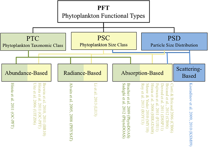
Figure 1. Schematic of various phytoplankton functional type (PFT) algorithms grouped according to their output classification (PTC, PSC, or PSD) and algorithm development types (abundance-, radiance-, absorption-, and scattering-based). Color indicates the output classification of phytoplankton taxonomic class (PTC, green), phytoplankton size class (PSC, yellow) or particle size distribution (PSD, blue).

TABLE 1

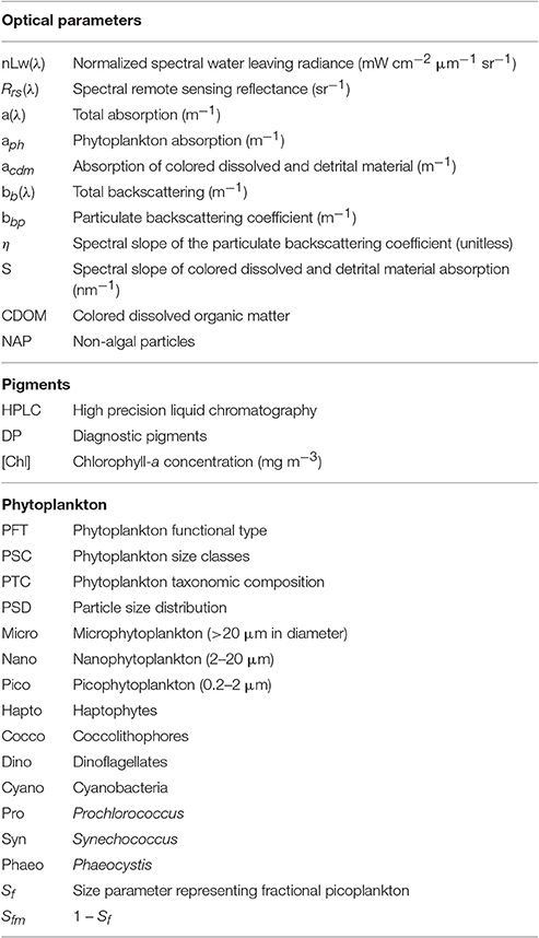
Table 1. Summary of notation (units in parentheses, where applicable).

Understanding Satellite Data Inputs: Ocean Color Radiometry

A satellite ocean color radiometer measures light (radiance) at the top of the atmosphere. On the global scale, the atmosphere alone typically accounts for >90% of this signal (Mobley, 1994). After atmospheric correction, the primary measured variable is spectral remote sensing reflectance [R_rs(λ)] or normalized water-leaving radiance [nLw(λ)]. [Note that these variables are related via R_rs(λ) = nLw(λ)/F₀(λ), where F₀(λ) is the extraterrestrial solar irradiance centered at wavelength λ (Thuillier et al., 2003)]. In open ocean waters, the threshold of uncertainty acceptance for R_rs(λ) is 5% (Bailey and Werdell, 2006). All other ocean color variables are estimated from R_rs(λ) (Figure 2). This means that the inherent optical properties (IOPs, i.e., absorption and scattering/backscattering), which are independent from the ambient light field, as well as, biogeochemical variables such as chlorophyll-a concentration, [Chl], are estimated from R_rs(λ), not measured directly from space. Approximate relationships between R_rs(λ) and IOPs were presented by Gordon et al. (1988) so that:

\begin{matrix} R_{r s} ​ (λ) = ℜ \frac{f (λ)}{Q (λ)} \frac{b_{b} (λ)}{a ​ (λ) + b_{b} (λ)} & (1) \end{matrix}

where, a(λ) is spectral total absorption coefficient and b_b(λ) is spectral total backscattering coefficient, ℜ is a factor that accounts for reflection and refraction at the air-water interface, and f/Q accounts for the bidirectional nature of reflectance (Morel et al., 2002). The IOPs absorption and backscattering are functions of biological/biogeochemical variables. Phytoplankton abundance, composition and physiological status impact [Chl], PSD, light absorption, and backscattering, and thus R_rs(λ). The algorithms that utilize absorption and backscattering satellite inputs obtain these IOP parameters from a variety of different semi-analytical inversion algorithms that are all fundamentally derived from the basic construct of Equation (1; Werdell et al., 2013; Figure 2). In contrary, the Phytoplankton Differential Optical Absorption Spectroscopy (PhytoDOAS) algorithm uses top of atmosphere satellite reflectance directly as input, to fit (and separate) simultaneously all absorbers in the atmosphere and ocean—accounting for atmospheric affects within the algorithm (Bracher et al., 2009; Sadeghi et al., 2012a).

FIGURE 2

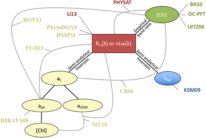
Figure 2. Schematic of satellite product inputs utilized in each PFT algorithm. The red box indicates the R_rs(λ) measured by a satellite radiometer. Ovals are derived satellite products and their connection to R_rs(λ) is indicated as black lines. Gray lines indicate the connection of satellite input products used in the various PFT algorithms. The color of the algorithm abbreviation text indicates the algorithm type: abundance (green), radiance (red), absorption (yellow) and scattering (blue). Algorithm abbreviations are as in Figure 1 and Tables 2, 3.

Abundance-based algorithms use [Chl] as a satellite input (Figure 2). To date, all published abundance-based models utilize [Chl] derived by an empirical approach (O'Reilly et al., 1998),

\begin{matrix} l o g_{10} [C h l] = a_{0} + \sum_{i = 1}^{4} a_{i} l o g_{10} {(\frac{R_{r s} (λ_{b l u e})}{R_{r s} (λ_{g r e e n})})}^{i} & (2) \end{matrix}

where, a₀–a₄ are sensor-specific coefficients and R_rs(λ_blue) is the greatest of several input R_rs(λ) values. However, within the constructs of the PFT algorithms, there is no reason why semi-analytically determined [Chl] could not be used in place of empirically determined [Chl]. The sensor-specific coefficients and bands are available at: http://oceancolor.gsfc.nasa.gov/cms/atbd/chlor_a. The level of acceptable uncertainty for [Chl] is 35% (Bailey and Werdell, 2006).

Within the portion of the satellite R_rs(λ) signal that is attributed to phytoplankton (absorption by pigments and scattering by cellular material), pigment abundance is primarily responsible for first order magnitude variability in R_rs(λ), while spectral shape differences associated with diversity in the taxonomic composition are secondary (Ciotti et al., 1999). Therefore, it is important to consider the overall phytoplankton contribution to total absorption and scattering budgets. Mouw et al. (2012) quantified this by looking at model output over the range of optical variability encountered in the global ocean considering scenarios where phytoplankton size did and did not vary. They find the magnitude of the [Chl] contribution to R_rs(443) (443 nm is the wavelength where greatest phytoplankton absorption occurs) is much greater than the contribution of phytoplankton taxonomic composition to R_rs(443) variability (see their Figures 6–8). This is due to the fact that chlorophyll-a, a pigment ubiquitous to all phytoplankton, has maximum absorption at 443 nm. PFT algorithms that exploit these second order characteristics, after accounting for the presence of colored dissolved organic matter (CDOM) and non-algal particles (NAP), are therefore subject to limitations due to relatively low signal-to-noise ratio of the residuals, that is, they operate near the limits of what is retrievable by the current state-of-the-art (e.g., Evers-King et al., 2014). Conversely, PFT algorithms that use the dominant abundance signal, such as [Chl], phytoplankton absorption, or particulate backscatter, are less impacted but have to face other limitations such as uncertainty in relationships between these properties and phytoplankton grouping.

Understanding Satellite PFT Outputs: PSC, PTC, and PSD

Here, we seek to summarize and simplify the satellite phytoplankton functional type algorithm products or outputs. The PSC output is most commonly grouped as pico- (0.2–2 μm), nano- (2–20 μm), and/or microplankton (>20 μm) following the size classification scheme proposed by Sieburth et al. (1978). However, a few models allow for multicomponent size classes not constrained by the traditional size groupings (Roy et al., 2013; Brewin et al., 2014b). The PSD satellite output (Kostadinov et al., 2009, 2010; Roy et al., 2013) can conform to the Sieburth et al. (1978) size classification. The PTC algorithms have a variety of outputs, dictated largely by the resolution of information available from in situ calibration and/or validation datasets. The PHYSAT approach (Alvain et al., 2005, 2008; Ben Mustapha et al., 2014) retrieves nanoeukaryotes, haptophytes (a major component of the nano-flagellates), Prochlorococcus, Synechococcus-like cyanobacteria, diatoms, coccolithophores, and Phaeocystis-like phytoplankton. The Hirata et al. (2011) approach retrieves pico-eukaryotes, prymnesiophytes (synonymous with haptophytes), diatoms, prokaryotes, green algae (chlorophytes), dinoflagellates, and Prochlorococcus sp., in addition to the main pico, nano, and micro size classes. The PhytoDOAS algorithm (Bracher et al., 2009; Sadeghi et al., 2012a) retrieves cyanobacteria, diatoms, coccolithophores, and dinoflagellates. We group similar classes together for clarity and simplicity. For example, haptophytes retrieved by Alvain et al. (2005, 2008) and Sadeghi et al. (2012a) are grouped with prymnesiophytes retrieved by Hirata et al. (2011). Prochlorococcus and Synechococcus, along with the broader prokaryotes class obtained by Hirata et al. (2011), are grouped as cyanobacteria (Table 2). Algorithm abbreviations follow those established by the algorithm's author(s), are consistent with those in Kostadinov et al. (2017), and are noted in Figure 1 and Table 2.

TABLE 2

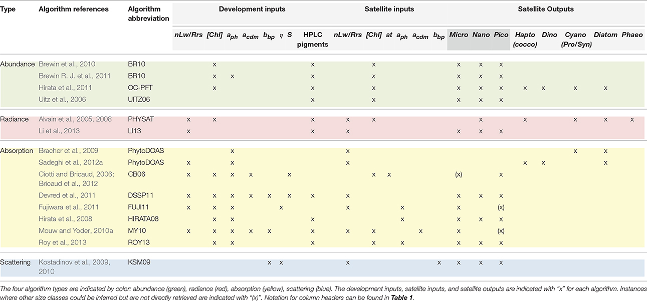
Table 2. Summary of satellite inputs and outputs.

These PFT output products are similar but are not identical and are defined by distinct units. These include dominance, [Chl] for each group (mg m⁻³), fractional [Chl] (%), fractional biovolume (%), absorption (m⁻¹) of each group, and a continuous size parameter varying from 0 to 1 (see Equation 1 and Table 3). We also simplify output with regards to units. All phytoplankton groups or size classes, regardless of units, are grouped together in Table 2 and Figure 3, which provide an overview of all algorithms. While users will most certainly require unit information, the overview table allows easy identification of the citations for the outputs of interest. For greater depth of information regarding units, a full list of output products, their validation source, and validation metrics are provided in Table 3.

TABLE 3

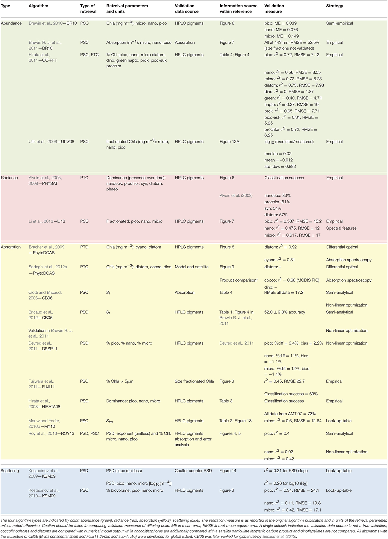
Table 3. Algorithm retrieval parameters and validation metrics.

FIGURE 3

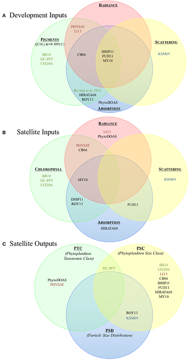
Figure 3. Schematic of parameter space utilized in algorithm development, as well as satellite input and output products. (A) Overview of the parameters utilized in development of the four algorithm types. The primary optical data types are indicated with colored circles: pigments (green), radiance (red), absorption (blue), and scattering (yellow). (B) Overview of the satellite input products for the four algorithm types. Satellite input products are indicated by the colored circles: radiance (red), chlorophyll concentration (green), absorption (blue), and scattering (yellow). Overlapping circles indicate two or more satellite input products are utilized. (C) Overview algorithms satellite output by PFT types. The colored circles indicate the PFT type of the output products (phytoplankton taxonomic class (PTC, green), phytoplankton size class (PSC, yellow), and particle size distribution (PSD, blue). Overlapping circles indicate where a given algorithm produces two or more satellite output product types. The color of the text in all subplots indicates the algorithm type: abundance (green), radiance (red), absorption (black) and scattering (blue). Algorithm abbreviations are as in Figure 1 and Tables 2, 3.

An important consideration is the aspect of phytoplankton group dominance. Alvain et al. (2005, 2008) and Hirata et al. (2008) retrieve the dominant group for a given satellite image pixel. Alvain et al. (2005) define dominance as situations in which a given phytoplankton group is the major contributor to the radiance anomaly. This contribution is retrieved as dominant when the ratio (biomarker pigment concentration/[Chl]) value is at least equal to 50% of the value that will be observed if the phytoplankton group was alone in the sample. This approach allows an empirical relationship between radiances anomalies and in situ information. For this reason, PHYSAT interpretation needs to be carefully considered in terms of in situ data used to give a name to the remotely sensed signal. Alvain et al. (2005) classify daily images and compile monthly maps of the most frequent dominant phytoplankton group. The group present in more than half of the daily images is assigned as dominant in the monthly compilation. When no group remains dominant over the whole month, pixels are labeled as unidentified. Hirata et al. (2008) determine PSCs from diagnostic pigments and relate them to phytoplankton absorption at 443 nm [a_ph(443)] to retrieve PSCs from satellite imagery. In the development stage of relating diagnostic pigments to a_ph(443) in situ, a PSC is defined as dominant if the marker pigment to diagnostic pigment ratio is >45%. However, in applying the approach to a_ph(443) imagery, PSCs are determined based on threshold ranges of a_ph(443), as such for a given pixel, only a single dominant type output is classified, regardless of temporal resolution of the satellite imagery. These are considerations users need to be aware of and can impact their interpretation and use. Further, when comparing satellite algorithms with biogeochemical model outputs, dominance (highest percentage of group) will vary whether one considers dominance of [Chl], a_ph(λ), b_bp(λ), or carbon—requiring care to ensure comparisons are done on the same terms.

Algorithm Basis

Abundance-based algorithms are based on the general observation that in the global open ocean a change in [Chl] is associated with a change in phytoplankton composition or size structure. The basis of this approach is that there is an upper limit of [Chl] in small cells imposed from genotypic and phenotypic constraints. Beyond this value, larger phytoplankton are responsible for an increase in [Chl] (Yentsch and Phinney, 1989; Chisholm, 1992).

Morel and Berthon (1989) suggested near surface [Chl] is related to water column-integrated chlorophyll content and its vertical distribution. Extending this work, Uitz et al. (2006) proposed quantitative relationships between the near surface [Chl] and (i) the water-column integrated chlorophyll content, (ii) its vertical distribution, and (iii) its community composition in terms of three pigment-based PSC. The relationships were established from the analysis of a large high precision liquid chromatography (HPLC) pigment database, covering a broad range of trophic conditions in the global open ocean. Uitz et al. (2006) used a modified version of the diagnostic pigment indices of Vidussi et al. (2001) (described in the Algorithm Validation Section) to determine the depth-resolved contribution to the total chlorophyll biomass of three PSCs (pico-, nano-, and microphytoplankton). The resulting PSC-specific vertical profiles of [Chl] from stratified waters were discriminated from those sampled in well-mixed waters based on the ratio of the euphotic layer depth (calculated from the vertical [Chl] profile following Morel and Maritorena, 2001) and the mixed layer depth (extracted from a global monthly climatology). For the stratified and mixed waters, the [Chl] profiles of pico-, nano-, and microphytoplankton were sorted in trophic categories, defined by successive intervals of surface [Chl]. For each trophic category, average profiles of [Chl] associated with the pico-, nano, and microphytoplankton were calculated. The shape and magnitude of these profiles showed regular changes along the trophic gradient and, thus, could be parameterized as a function of surface [Chl]. Applied in a continuous manner to any given satellite-derived surface [Chl], the resulting empirical parameterization enables the ability to derive a vertical profile of [Chl] for each of the three pigment-based PSCs.

Hirata et al. (2011) estimate fractions of three PSCs and seven PTCs from empirical relationships between [Chl] and diagnostic pigments of various phytoplankton groups (see equations and coefficients in Hirata et al., 2011), based on global observations that abundance and composition of phytoplankton are not necessarily independent/de-coupled on synoptic scale. Brewin et al. (2010), extending the model proposed by Sathyendranath et al. (2001), describe the exponential functions that relate [Chl] to the fractional contribution of various PSCs,

\begin{matrix} {[C h l]}_{p, n} = C_{p, n}^{m} [1 - \exp (- S_{p, n} [C h l])] & (3 a) \end{matrix}

\begin{matrix} {[C h l]}_{p} = C_{p}^{m} [1 - \exp (- S_{p} [C h l])] & (3 b) \end{matrix}

\begin{matrix} {[C h l]}_{n} = {[C h l]}_{p, n} - {[C h l]}_{p} & (3 c) \end{matrix}

\begin{matrix} {[C h l]}_{m} = [C h l] - {[C h l]}_{p, n} & (3 d) \end{matrix}

where subscripts p, n, and m refer to pico- (>0.2–2 μm), nano- (>2–20 μm), and microplankton (>20 μm), respectively. $C_{p, n}^{m}$ and $C_{p}^{m}$ are asymptotic maximum values for the associated size classes and S_{p, n} and S_p determine the increase in size-fractionated [Chl] (parameter values can be found in Table 2 of Brewin et al., 2015), and have been found to vary with environmental conditions (Brewin et al., 2015; Ward, 2015). Both Brewin et al. (2010, 2012), Brewin R. J. W. et al. (2011) and Hirata et al. (2011) utilize the continuum of [Chl] (please see Figure 2 in Hirata et al., 2011 and Figure 4A in Brewin et al., 2010).

Radiance-based algorithms classify PFTs based on the shape and/or magnitude or the satellite-observed R_rs(λ) or nLw(λ). Radiance-based approaches assume that, after normalization, changes in radiance coincide with changes in PFT composition, as opposed to other in-water constituents such as CDOM or NAP that may or may not covary with the phytoplankton (e.g., Siegel et al., 2005). Alvain et al. (2005, 2008) normalize R_rs(λ) to [Chl] and identify characteristic spectral bounds for several PTCs in terms of shape and amplitude (Ben Mustapha et al., 2014): nanoeukaryotes, Prochlorococcus, Synechococcus-like cyanobacteria, diatoms, Phaeocystis-like cells, and coccolithophores. More recently, based on theoretical relationships between radiance anomalies and specific phytoplankton groups, PHYSAT has been shown to potentially detect phytoplankton assemblages of several PTC as opposed to a single dominant one (Rêve et al., in revision). Alternatively, Li et al. (2013) consider a variety of spectral features on surface reflectance and use machine learning to select the most significant of these. They find continuum-removed and spectral curvature are the most significant spectral features with particular importance around 440–555 nm, which isolate absorption characteristics and measure non-linearity. They utilize these results with support vector regression to estimate PSCs.

Absorption-based algorithms comprise by far the majority of existing approaches. All of the approaches have some level of dependence on the spectral magnitude or shape of phytoplankton absorption [a_ph(λ)]. The magnitude of a_ph(λ) is related to pigment composition and total pigment concentration, dominated by [Chl] at the peak wavelength (for oceanic waters) of 443 nm. Size information is contained in the absorption spectrum due to pigment packaging (e.g., Bricaud and Morel, 1986). Some of the approaches utilize chlorophyll-specific phytoplankton absorption in which phytoplankton absorption is normalized to [Chl] (Bracher et al., 2009; Mouw and Yoder, 2010a; Sadeghi et al., 2012a; Roy et al., 2013), either for a specific wavelength or to derive a spectral shape or slope that is related to second order signals including pigment composition and packaging. Several of the approaches (Ciotti and Bricaud, 2006; Mouw and Yoder, 2010a; Bricaud et al., 2012) stem from the theoretical underpinning of Ciotti et al. (2002) who identify that, despite the physiological and taxonomic variability, variation in a_ph(λ) spectral shape can be defined by changes in the dominant size class. They determine chlorophyll-specific phytoplankton absorption ( $a_{p h}^{*}$ ) as weighted between normalized mean pico- ( $ā_{p h, p i c o}^{*}$ ) and microplankton ( $ā_{p h, m i c r o}^{*}$ ) chlorophyll-specific absorption spectra.

\begin{matrix} a_{p h}^{*} (λ) = [S_{f} \times {\bar{a}}_{p h, p i c o}^{*} (λ)] + [(1 - S_{f}) \times {\bar{a}}_{p h, m i c r o}^{*} (λ)] & (4) \end{matrix}

where S_f is a dimensionless index constrained to vary between 0 and 1, specifying the relative contributions of microphytoplankton and picophytoplankton, respectively, to phytoplankton absorption. Equation (4) is based on the fact that the shape of the phytoplankton absorption spectrum flattens with increasing cell size. This relationship results from pigments being contained within particles (rather than in solution), known as the “discreetness effect,” and secondarily how pigments are packaged within the cell, known as the “packaging effect” (Morel and Bricaud, 1981). Small cells have little cellular material between the chloroplast and cell wall making them highly efficient absorbers, resulting in higher magnitude and more peaked absorption. With large cells, light has to penetrate more cellular material to reach the chloroplast after passing through the cell wall, resulting in muted absorption affinity and in some cases shelf-shading (see Figure 7E in Ciotti et al., 2002). Note that the shape of the phytoplankton absorption spectrum (and therefore the S_f-value) can be affected by variations in pigment composition and intracellular pigment concentration resulting from photoacclimation, independent of cell size. Ciotti and Bricaud (2006) proposed a new $ā_{p h, p i c o}^{*}$ vector, based on an oceanic data set and Bricaud et al. (2012) utilize this relationship directly to retrieve S_f, absorption due to non-algal particles and colored dissolved organic matter at 443 nm [a_dg(443)] and the spectral slope of a_dg(λ) through an inversion model. Mouw and Yoder (2010a) modify Equation (4) to vary with the percentage of microplankton (S_fm) rather than picoplankton. They develop an optical look-up-table (LUT) that contains ranges of S_fm, [Chl], and a_dg(λ) from which R_rs(λ) is calculated from radiative transfer. They utilize satellite [Chl] and a_dg(443) to narrow the search space within the LUT, then find the closest match between satellite R_rs(λ) and LUT R_rs(λ) and retrieve the associated S_fm from the LUT.

Hirata et al. (2008) do not use the Ciotti et al. (2002) construct (i.e., Equation 4) that utilizes multiple wavelengths to characterize the spectral shape of a_ph(λ). Instead, they identify a tight relationship between the magnitude of phytoplankton absorption at a single wavelength [a_ph(443)], related to [Chl], and the slope of a_ph(443) to a_ph(510), which is influenced by pigment packaging and composition. When this approach is applied to satellite data, it only uses a_ph(443), and determines dominate size class using boundaries in a_ph(443).

The approaches of Devred et al. (2011) and Brewin R. J. W. et al. (2011) are similar to that of Brewin et al. (2010), applying the constructs of Equations (3a–3d). Devred et al. (2011) use Equation (3) to derive chlorophyll-specific absorption coefficients for three PSCs. When this approach is applied to satellite data, it uses a semi-analytic inversion algorithm together with the derived chlorophyll-specific absorption coefficients to estimate size-fractionated [Chl], not using Equation (3) at this stage; hence this approach does not assume covariance between total [Chl] and size-fractionated [Chl] (as with an abundance-based approach). Fujiwara et al. (2011) is the only absorption-based approach that also uses backscatter as an input, which they determine empirically from R_rs(λ) band ratios. They estimate PSC utilizing empirical relationships with phytoplankton absorption-spectra ratios and the particulate backscatter slope.

Roy et al. (2011) developed a semi-analytical algorithm based on phytoplankton absorption at a red wavelength (676 nm) to compute the equivalent spherical diameter of phytoplankton. Roy et al. (2013) further extended the algorithm to heterogeneous phytoplankton populations, where they utilized phytoplankton absorption at 676 nm to compute the PSD corresponding to the phytoplankton cells alone, and derived the power-law exponent/slope of the phytoplankton size spectrum. Knowing the slope of the phytoplankton cell-size distribution, the proportions of [Chl] within any diameter range of PSCs can be calculated.

The PhytoDOAS algorithm (Bracher et al., 2009; Sadeghi et al., 2012a) uses hyperspectral top of atmosphere reflectances to identify spectral features associated with PTCs. This approach requires hyperspectral satellite data and has been applied to the SCanning Imaging Absorption SpectroMeter for Atmospheric CHartographY (SCIAMACHY) onboard ENVISAT (more details in Bovensmann et al., 1999), which has a limited spatial coverage and resolution with 6-day revisit and 30 by 60 km pixel size. The differential optical absorption spectroscopy (DOAS) technique exploits sharp spectral features and when extended to phytoplankton, differentiates on spectral specific-absorption features of major PTCs. The DOAS method, utilizes observed backscattered radiation, normalized to the solar irradiance, at the top of the atmosphere and absorption cross sections (i.e., specific absorption coefficients, of all important absorbing constituents varying spectrally in the atmosphere-ocean system). The method uses non-linear optimization to fit these “differential absorption cross sections” of different phytoplankton groups, water vapor, and atmospheric trace gases: O₃, O₄, NO₂, glyoxal (CHOCHO), iodine oxide (IO), and spectral features caused by filling-in of Fraunhofer Lines due to Raman scattering. The contributions of broad-band scattering and absorption features, such as Mie- and Ray-leigh scattering in the atmosphere or NAP and CDOM in water, are approximated by a second-order polynomial in each fit. Bracher et al. (2009) adopted DOAS within 429–495 nm to retrieve absorption and biomass of cyanobacteria and diatoms independently. Sadeghi et al. (2012a) extended the method further to simultaneously retrieve diatoms, coccolithophores, and dinoflagellates over the 429–521 nm spectral range.

To date, there have only been two scattering-based algorithms published. Backscattering approaches retrieve information on all particles rather than just phytoplankton. Generally, the backscattering coefficient decreases according to a power law function with increasing wavelength. Smaller particles have a greater backscattering slope (η) than larger particles. Montes-Hugo et al. (2008) was the first to estimate phytoplankton size by considering the backscattering slope. They demonstrated their approach near the western shelf of the Antarctic Peninsula. Kostadinov et al. (2009) was the first to demonstrate the approach globally. They estimate spectral particulate backscattering [b_bp(λ)] from R_rs(λ) and then calculate η from b_bp(λ) based on Loisel et al. (2006). Using η, the PSD slope and reference abundance of particles are retrieved from a look-up-table that is constructed based on theoretical Mie scattering computations. These parameters are then used to estimate the number and volume concentrations for pico, nano, and micro sized particles. Assuming the relative proportions of biovolume are roughly constant across size classes, Kostadinov et al. (2010) validate the Kostadinov et al. (2009) approach with pigments and confirm pigment-based micro-, nano-, and pico-sized phytoplankton approximately represent micro-, nano-, and pico-sized particles derived from backscattering. Kostadinov et al. (2016a) further develop the KSM09 approach by using existing allometric relationships (Menden-Deuer and Lessard, 2000) to convert bio-volume calculated from the PSD to phytoplankton carbon (C) in these three PSCs. These PSCs are the only carbon-based PFT retrievals available to date. The approach can be used to estimate phytoplankton carbon concentrations (absolute and fractional) in any size class in the 0.5–50 μm diameter range. It is desirable to express the PFTs in terms of carbon because: it is relatively insensitive to variations in phytoplankton physiological, unlike [Chl]; it is relevant to the carbon cycle and other biogeochemical cycles; and carbon is the unit used for PFTs in climate models (Hood et al., 2006).

Algorithm Validation

Nearly all algorithms are validated against estimates of phytoplankton size and composition estimates determined from in situ measurements of pigment concentrations with the HPLC technique (Table 3). The chemotaxonomic approach provides a means to quantify phytoplankton taxonomic composition utilizing a set of biomarker pigments (e.g., Jeffrey et al., 1997; Roy et al., 2011). Claustre (1994) and Vidussi et al. (2001) further proposed to utilize groupings of biomarker pigments to estimate phytoplankton size structure. They identified a set of seven diagnostic pigments specific to phytoplankton taxa, which were then assigned to one of the three size classes (micro-, nano-, and pico-) depending on the average cell size of the organisms. The diagnostic pigment-based approach enables estimating the contribution of the three phytoplankton size classes to the total chlorophyll a biomass as follows (Equation 5):

\begin{matrix} Σ D P = \sum_{i = 1}^{1} W_{i} P_{i} & (5 a) \end{matrix}

\begin{matrix} f_{m i c r o} = \frac{\sum_{i = 1}^{2} W_{i} P_{i}}{Σ DP} & (5 b) \end{matrix}

\begin{matrix} f_{n a n o} = \frac{\sum_{i = 3}^{5} W_{i} P_{i}}{Σ DP} & (5 c) \end{matrix}

\begin{matrix} f_{p i c o} = \frac{\sum_{i = 6}^{7} W_{i} P_{i}}{Σ DP} & (5 d) \end{matrix}

where, ΣDP is the sum of all the diagnostic pigments multiplied by the weight coefficients (W_i, values discussed below), f_micro, f_nano, and f_pico are the fractions of the micro-, nano- and pico-plankton size classes to [Chl], and P_i are the pigments' concentrations (P = {fucoxanthin; peridinin; 19′-hexanoyloxyfucoxanthin; 19′-butanoyloxyfucoxanthin; alloxanthin; chlorophyll-b and divinyl chlorophyll-b; zeaxanthin}). The most widely used coefficients are those proposed by Uitz et al. (2006) (W = {1.41; 1.41; 1.27; 0.35; 0.6; 1.01; 0.86}), which were derived from a global HPLC pigment database.

While diagnostic pigments have been widely used for validation due to the availability of extensive datasets of HPLC pigments across the global ocean (Peloquin et al., 2013), there are important limitations to consider. The diagnostic pigment-based approach does not necessarily reflect the true size structure of the phytoplankton communities because some taxonomic groups may spread over a broader size range (e.g., diatoms are typically found in the micro- but could also occur in the nano-size and sometimes in the pico-size classes) and some diagnostic pigments are shared by different taxonomic groups (e.g., fucoxanthin is the main carotenoid of diatoms but may also be found in prymnesiophytes). Recently modifications to the Vidussi et al. (2001) and Uitz et al. (2006) approach were proposed that account for the presence of some diagnostic pigments in more than one taxon. Hirata et al. (2011) and Devred et al. (2011) proposed further adjustments to the fucoxanthin pigment coefficient, to assign a portion of this pigment to nanoplankton. To address the analogous issue that prymnesiophytes predominate within the nanophytoplankton but can also be present in the pico-eukaryote population, Brewin et al. (2010) modified the 19′-hexanoyloxyfucoxanthin (19′-hex) coefficient to attribute a portion of this pigment to the picoplankton in low [Chl] waters. Furthermore, the DP for diatoms, fucoxanthin, is the precursor pigment for 19′-hex leading to some prymnesiophytes being classified as diatoms. For the algorithms that utilize HPLC pigments in their development, it should be noted that direct comparisons need to be considered carefully, as not all output products are developed and validated with the same set of diagnostic pigment coefficients. There are ongoing efforts to verify HPLC methods (i.e., Equation 5) through comparison with other techniques (e.g., Brewin et al., 2014a). As Nair et al. (2008) pointed out, any single method alone may not be entirely dependable, thus incorporating various methodologies leads to a more complete diagnosis of phytoplankton groups. Future efforts are necessary to complement HPLC methods with independent information on PFTs, for instance carbon-based size classes (Kostadinov et al., 2016a).

Not all validation approaches are based on HPLC pigment data, but rather use information on either absorption coefficients (Ciotti and Bricaud, 2006; Brewin R. J. W. et al., 2011) or size-fractionated [Chl] (Fujiwara et al., 2011). In addition, the study of Sadeghi et al. (2012b) does not perform a true validation, but rather compares numerical model results to other satellite products (Table 3).

Validation metrics are not reported using uniform metrics across algorithms causing an additional layer of complication when comparing algorithm performance. While it would be better to provide consistent validation measures across all algorithms, as mentioned previously, different satellite product outputs, units and use of variable development and validation datasets/coefficients, preclude this ability. Reported validation measures are compiled in Table 3. Ideally, root mean square error (RMSE) (IOCCG, 2006) should be reported for matchups carried out according to the methods of Bailey and Werdell (2006) that specify the mean value of a five-by-five pixel box at the highest available pixel resolution measured by the sensor surrounding the location and within ±3 h of an in situ observation. In many cases, 9 km global area coverage satellite data are used to infer PFT classification. Thus, the spatial resolution is already coarse for validation matchups. However, algorithms can also be applied to full resolution (1 km) imagery improving validation efforts. In the case of PhytoDOAS, the input requires hyperspectral resolution and has been developed for use with SCIAMACHY, which has a resolution of 30 by 60 km. Spatial resolution differences between in situ point observations and the large SCIAMACHY pixels presents a limitation for validation using matchups (Bracher et al., 2009), since only very few in situ observations are within a homogeneous area of the size of a SCIAMACHY pixel. However, Aiken et al. (2007) point out that in the open ocean phytoplankton assemblages may be homogenously distributed over 50–100 km and smaller scales are possible for specific communities. In Sadeghi et al. (2012b), PhytoDOAS coccolithophore [Chl] was validated by comparison with satellite-derived particulate inorganic carbon (Balch et al., 2005).

Algorithm Selection

Users often select satellite products that most closely align with their application. When there are several satellite product choices for a given PFT type with varying facets and complexity, the optimal choice may not be clear. To help users determine what might be best suited for their purpose, in addition to the satellite inputs, outputs, and validation metrics described above, we compile a comparative list of assumptions, strengths, and limitations (Table 4). It is possible that merged products produce the best output beyond any individually selected algorithm (Palacz et al., 2013), yet an understanding of the underlying inputs into a merged product is always desirable.

TABLE 4

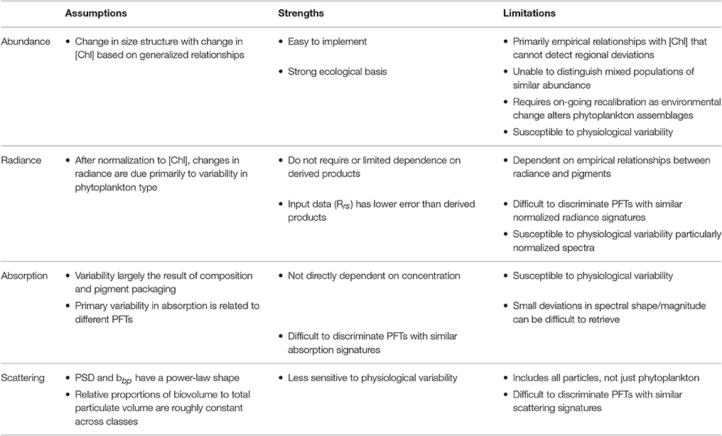
Table 4. Comparative summary of algorithm assumptions, strengths and limitations.

Abundance-based algorithms assume a change in size and taxonomic structure with a change in chlorophyll. To the first order, and for large time and space scales, this holds true, but there are exceptions. Deviations from the mean state of the data in which the relationship is developed may occur (Hirata et al., 2011). This is particularly challenging at regional scales and in optically complex water where CDOM and NAP also complicate the retrieval of [Chl]. In a changing ocean, if shifts toward different phytoplankton assemblages with similar [Chl] occur, empirical relationships will require recalibration (Hirata et al., 2011). Abundance-based algorithms begin with uncertainty associated with the input satellite [Chl] product in addition to the uncertainty in relationships between [Chl] and phytoplankton grouping (Figure 2). Typically, band-ratio estimation of [Chl] (O'Reilly et al., 1998) has an accepted 35% uncertainty (Bailey and Werdell, 2006), which has recently been documented to be much less in the open ocean (16%) (Brewin et al., 2016), but becomes worse in coastal waters. Some semi-analytical inversions that retrieve [Chl], also have similar uncertainty across global scales (Brewin et al., 2015), but may maintain accuracy in coastal waters due to their ability to account for other in-water constituents contributing to the IOPs present that vary independently of each other. However, PFT approaches, which are broadly characterizing phytoplankton, may ultimately result in less uncertainty than the starting [Chl] product. The attractiveness of the abundance-based approaches is their ease of implementation and that they exploit the first-order signal in R_rs. [Chl] a primary biological variable that is routinely measured in situ, thus enabling extensive association of PFT fields with the abundance of in situ [Chl] that has accumulated across the globe. Once you know [Chl], PSC, or PTC estimates are a simple calculation.

Radiance-based approaches assume that after normalization to [Chl], changes in radiance coincide with changes in PFTs. They utilize R_rs(λ) [or nLw(λ)], the fundamental parameter observed by a satellite radiometer and having uncertainty thresholds of 5% (Bailey and Werdell, 2006). Thus, the strength of radiance-based approaches is that they do not require or have limited dependence on products derived from R_rs(λ). However, any normalization of the signal to derive the second-order relationships that tend to underpin these approaches will inevitably suffer from reduced signal to noise. Furthermore, when [Chl] is used in normalization (e.g., PHYSAT), the uncertainty associated with [Chl] is introduced (Figure 2). These algorithms are dependent on empirical relationships between radiance and PTCs or PSCs, thus as with empirical [Chl] dependencies described above, they require recalibration for long-term analyses. As with absorption- and scattering-based approaches and abundance-based approaches when using [Chl] determined from a semi-analytical model, radiance-based approaches allow for the ability to account for other optically active in water constituents (CDOM and NAP) as these also impact the spectral radiance (Alvain et al., 2012). This aspect allows potential development by users who have their own in situ datasets—it is possible to empirically associate a specific radiance anomaly to phytoplankton assemblages or specific composition (Alvain et al., 2012; Rêve et al., in revision). This highlights the importance of continued investment of detailed in situ databases to allow future development and use of remotely sensed phytoplankton groups. Radiance-based approaches are also influenced by physiological variability; however, the variability likely represents a larger proportion of the signal in normalized quantities.

PhytoDOAS (Bracher et al., 2009; Sadeghi et al., 2012a) has so far only been applied to a single sensor that has sufficient spectral resolution, precluding it from studies of phytoplankton composition where 30 km spatial resolution would be limiting. However, this is expected to improve in the near future: adaptations of the algorithm to similar high spectrally resolved satellite data with improved spatial coverage and resolution are currently ongoing. Ozone Monitoring Instrument (OMI) (since 2004) with 13 km by 24 km and TROPOMI (tropospheric OMI, to be launched in early 2017) with 3.5 km by 7 km global spatial resolution are, or will be, used with PhytoDOAS. In addition, ocean color sensors are planned for the future with significantly increased spectral resolution (Mouw et al., 2015) that may allow a wider adoption of the PhytoDOAS method to even smaller spatial scales. For example, NASA's planned Plankton, Aerosol, Cloud, and ocean Ecosystem (PACE) mission with a hyperspectral ocean color sensor payload is expected to revolutionize the ability to use algorithms, such as PhytoDOAS, on more adequate spatio-temporal scales.

The number of existing absorption-based algorithms indicates the clear impact phytoplankton cell size and pigment composition have on the shape of the spectral absorption coefficient. These relationships have been reported in the literature for decades (e.g., Bricaud et al., 1988, 1995; Ciotti et al., 1999). The strengths of this type of algorithm include the ability to begin with inherent optical properties rather than [Chl] as the satellite input product, thus starting with reduced uncertainty at the onset. However, the assumed spectral shapes and coefficients utilized in semi-analytical approaches cannot fully capture natural variability across a variety of conditions resulting in uncertainties. These uncertainties are a balance of spectral accuracy and the accuracy of particular parameters over others (Werdell et al., 2013). As with R_rs approaches, those that require normalization by [Chl] inevitably reduce signal to noise and also reintroduce uncertainty associated with [Chl]. A limitation of absorption-based approaches is that they are sensitive to physiological variability associated with light and nutrient histories and these are likely to be of more influence when normalized quantities are used. Furthermore, small changes in the spectral shape of phytoplankton absorption can be difficult to retrieve from ocean-color (Garver et al., 1994; Wang et al., 2005), such that identifying and distinguishing different PFTs may not always be successful. Problems can also occur when trying to discriminate different phytoplankton groups with similar absorption signatures.

The scattering-based approaches presented here assume the PSD has a power-law shape and relative proportions of biovolume are roughly constant across size classes. Conversion to phytoplankton carbon for the carbon-based PFTs requires additional assumptions Kostadinov et al. (2016a). The models assume a relationship between the PSD and the spectral slope of b_bp(λ). The use of b_bp(λ) makes the approach less sensitive to physiological variability than other approaches. However, the particle size classes include all particles, not just phytoplankton and the relationship between b_bp(λ) and phytoplankton cell size is still a matter of active debate (Stramski et al., 2004; Vaillancourt et al., 2004; Dall'Olmo et al., 2009; Whitmire et al., 2010). In addition, the sources of backscattering are still uncertain (Stramski et al., 2004) and applicability of Mie theory to particles and/or phytoplankton assemblages in seawater has its limitations (e.g., Dall'Olmo et al., 2009). It has been suggested that this approach represents phytoplankton carbon more closely—see Martinez-Vicente et al. (2013), and backscattering has been used to retrieve total phytoplankton carbon (Behrenfeld et al., 2005).

Users are more focused on the satellite outputs, which they can use for various applications, rather than the intricacies of the type of algorithm used to produce the output. For ease of information identification, we have provided the validation metrics reported by algorithm type and satellite output types (Table 3). However, our purpose here is not to intercompare or validate algorithms. It is important to point out that the algorithms all use different approaches, datasets, and validation metrics. To be able to properly assess algorithm performance, one would have to carry out a comprehensive inter-comparison using the same validation data and consider errors of omission and commission (see Brewin R. J. et al., 2011), which is outside the scope of the present work. A validation effort is planned as part of the International Satellite Phytoplankton Functional Type Algorithm Inter-comparison Project (Hirata et al., 2012; http://pft.ees.hokudai.ac.jp/satellite/index.shtml) while an intercomparison based on phenology has been carried out by Kostadinov et al. (2017).

It is important to point out that many of these methods have been developed for the global open ocean. The optical complexity encountered in coastal waters is quite different from that found in the global datasets used to develop these algorithms. Additionally, the assumptions made by some are only valid for the global open ocean. The relationship between [Chl], CDOM absorption, and particulate backscatter is more variable in coastal water than the open ocean. For example, riverine sources, resuspension, and mixing may cause CDOM and NAP to vary independently of phytoplankton. For these reasons, band-ratio [Chl] estimates that utilize the blue and green region of the spectra are plagued with problems in coastal waters (Matthews, 2011). Thus, it is not advisable to apply open ocean abundance-based algorithms to coastal systems. Relationships would need to be assessed and likely redeveloped using a regionally specific dataset. Similar limitations would be expected for radiance-based methods. While the atmospheric correction can be a challenge over some coastal waters (Goyens et al., 2013), if R_rs(λ) is accurately retrieved, the dynamic range of CDOM and NAP that impart a significant signal to R_rs(λ) require empirical relationships and thresholds defined for various PFTs and PSCs to be reestablished. The approaches that build upon semi-analytic expressions that first retrieve IOPs from R_rs(λ) and then PFTs from the retrieved IOPs, have the greatest ability to accommodate dynamic environments. These approaches parse the contributions of NAP, CDOM and phytoplankton before the phytoplankton IOPs are associated with a PFT. Similarly, this is done within the PhytoDOAS method by accounting for all relevant absorbers (from water and atmosphere) within the fitting of hyperspectral top of atmosphere reflectance. Accordingly, Brewin R. J. et al. (2011) find absorption-based approaches show an improvement over abundance-based approaches in coastal waters. However, the thresholds of detectability of approaches targeting optical signatures will not allow PFT retrieval in all cases.

The limitation of the ability to retrieve PFTs in some cases needs to be acknowledged. For example, Mouw and Yoder (2010a) are careful to consider the change in R_rs(λ) produced by PSCs, [Chl] and CDOM absorption in relation to the radiometric sensitivity of the satellite senor. They find that when [Chl] or CDOM absorption were too high, the impact of size on R_rs(λ) is masked. Likewise, when [Chl] is too low, the spectral response of R_rs(λ) due to size is too small to differentiate from noise. Additionally, PHYSAT in its first version (Alvain et al., 2005) did not classify pixels where no phytoplankton group dominated due to the use of biomarker pigment threshold during the first empirical anomalies labeling steps. However, recent developments of PHYSAT have shown its capability to detect more than dominance cases utilizing detailed in situ data (Alvain et al., 2012; Ben Mustapha et al., 2014; Rêve et al., in revision).

The accessibility of products is another reason why users may select a given algorithm over another. Algorithms where simple calculations extracted from the publication can be quickly applied are far more likely to be utilized than those that require multiple complicated steps. The algorithm developer hosting the final output product for download by users has often remedied difficulty in this later situation. The PFT products that are currently accessible online are listed in Table 5. Further, the PFT products compiled for phenological comparison (Kostadinov et al., 2017) intend to be released in the near future. The availability of PFT product access is anticipated to grow substantially as future missions that have specified PFT products as part of their mission goals come online.

TABLE 5

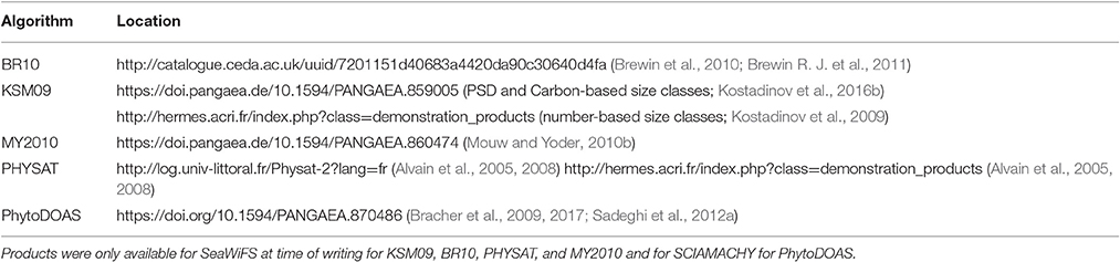
Table 5. Online availability of permanently archived PFT algorithm products.

PFT algorithm development thus far has been focused on retrieving global distributions of PFTs. The next challenge is to detect change in these distributions over time. The temporal anomaly of PFTs can be a smaller signal than the bulk composition retrievals achieved thus far. The anomalies are critical for understanding climate change issues and testing ecosystem model prediction. However, detecting change is confounded by inter- and intra-algorithm uncertainties and the relatively short record length of satellite data. Further, critical to this consideration are changes in phytoplankton physiology. Behrenfeld et al. (2016) show the importance of accounting for photoacclimation in temporal chlorophyll variability, as light-driven changes in chlorophyll can be associated with constant or increased photosynthesis. This finding of the necessity to account for physiological plasticity also directly impacts the PFT methods described here, most acutely for abundance-, radiance-, and absorption-based methods. While satellite PFT time series data have already been used to assess regional PFT variability and trends (Brewin et al., 2012; Sadeghi et al., 2012b; Alvain et al., 2013; Soppa et al., 2016). there is a need to characterize physiological plasticity in PFT retrievals to more accurately quantify phytoplankton compositional response to a changing ocean.

Conclusions

At the global scale, the current PFT algorithms demonstrate proof of concept in retrieving phytoplankton composition from satellite radiometry, opening the door for further development, and expand the use of satellite observations. While there are a variety of algorithm approaches, all agree on broad understanding of PFT distribution at large spatial-temporal scales, that are forced mainly by bathymetry and climatic regions. Larger cells and taxa tend to be found near coastal regions, especially under upwelling regimes, while smallest cells and taxa dominate in the center of oceans. Temperate regions are likely to present seasonal blooms of large cell sizes in spring and/or fall, while a less variable size distribution of phytoplankton is expected in tropical and subtropical areas and in the oligotrophic gyres.

Continual PFT algorithm development is anticipated, particularly with the expansion of sensor capability with future missions. Planned capability will expand spectral, spatial, and temporal resolution, in addition to radiometric sensitivity (Mouw et al., 2015). Increased spectral resolution will provide the ability to exploit more spectral signatures of PFTs (Isada et al., 2015; Wolanin et al., 2016). In addition to increased spectral resolution, increased spatial resolution may lend clarity to coastal processes and phytoplankton response to finer scale physical features. Improved temporal resolution on geostationary platforms will allow multiple views per day to investigate diurnal phytoplankton variability. Improved radiometric sensitivity will expand threshold detection required to detect the secondary impact of PFTs on radiometric variability. All of the potential capability in expanded satellite PFT products with the next generation of satellite sensors hinges on continued and increased investment in in situ observations to allow further algorithm development and validation. In addition to HPLC pigments that so many of these approaches are validated upon, training datasets also need to include unambiguous metrics of community composition that include particle size distribution and taxonomy (from imaging technologies) (Bracher et al., 2015). Exploiting compilations of abundance and biomass (Leblanc et al., 2012) and connections to genetically determined community composition (Malviya et al., 2016) are potentially rich resources for expanding training and validation datasets. In addition, coincident optical [i.e., R_rs(λ) and IOPs] observations will be highly important to connect to the signals observed by satellite radiometers. The expanding optical sensors on Bio-Argo floats may also provide a valuable data stream for PFT development, particularly for vertical structure of phytoplankton communities (Mignot et al., 2014). It is important to expand the capability to measure phytoplankton carbon in situ (Graff et al., 2012, 2015) so future definitions of PFTs can be more carbon-relevant (Kostadinov et al., 2016a).

This document provides an overview of the primary components used in developing, implementing, and using satellite PFT products. While we do not provide direct recommendations for particular applications, our hope is that providing an accessible overview of the primary components of PFT algorithms will aid users in more confidently selecting products for a given application and ignite future conversations between satellite product developers and a variety of user communities. The satellite PFT literature is rapidly expanding and these tables and figures will require updating and the need to develop anew. In addition to the value we hope this brings to the user community, we equally hope this summary provides a framework for algorithm organization to inform where possible new approaches could be investigated into the future.

Author Contributions

CM carried out the synthesis of algorithms, developed the organization, and prepared the manuscript with guidance from NH. CM prepared all figures and tables. All other co-authors contributed to ensuring accuracy of their algorithm description, overall synthesis, and editing.

Funding

The National Aeronautics and Space Administration (NASA) provided financial support for CM (NNX13AC34G) and TK (NNX13AC92G) for this effort. The contribution of AsB, RB, and AnB was partly funded via the ESA SEOM SY-4Sci Synergy project SynSenPFT.

Conflict of Interest Statement

The authors declare that the research was conducted in the absence of any commercial or financial relationships that could be construed as a potential conflict of interest.

The handling Editor declared a shared affiliation, though no other collaboration, with several of the authors SA, AB, and JU and states that the process nevertheless met the standards of a fair and objective review.

Acknowledgments

We acknowledge the International Satellite Functional Type Algorithm Intercomparison Project (http://pft.ees.hokudai.ac.jp/satellite/) for facilitation of a series of meetings and workshops that led to the development of this manuscript, with funding from JAXA and the UK National Centre for Earth Observation and support from the International Ocean Colour Coordination Group (IOCCG).

References

Aiken, J., Fishwick, J., Lavender, S., Barlow, R., Moore, G., Sessions, H., et al. (2007). Validation of MERIS reflectance and chlorophyll during the BENCAL cruise October, 2002: preliminary validation of new products for phytoplankton function types and photosynthetic parameters. Int. J. Remote Sens. 28, 497–516. doi: 10.1080/01431160600821036

REVIEW article

A Consumer's Guide to Satellite Remote Sensing of Multiple Phytoplankton Groups in the Global Ocean

Introduction

Algorithm Overview

Understanding Satellite Data Inputs: Ocean Color Radiometry

Understanding Satellite PFT Outputs: PSC, PTC, and PSD

Algorithm Basis

Algorithm Validation

Algorithm Selection

Conclusions

Author Contributions

Funding

Conflict of Interest Statement

Acknowledgments

References

This article is part of the Research Topic

People also looked at