Uncertainty in Ocean-Color Estimates of Chlorophyll for Phytoplankton Groups

1. Introduction

The size structure and taxonomic composition of phytoplankton influence many processes in phytoplankton biology, marine biogeochemistry and marine ecology (Chisholm, 1992; Raven, 1998; Le Quéré et al., 2005; Marañón, 2009, 2015; Finkel et al., 2010). Photosynthesis, growth, light absorption, nutrient uptake, carbon export, and the transfer of energy through the marine food chain, are all influenced by phytoplankton community structure (Platt and Denman, 1976, 1977, 1978; Morel and Bricaud, 1981; Prieur and Sathyendranath, 1981; Probyn, 1985; Geider et al., 1986; Legendre and LeFevre, 1991; Maloney and Field, 1991; Chisholm, 1992; Sunda and Huntsman, 1997; Raven, 1998; Laws et al., 2000; Ciotti et al., 2002; Bricaud et al., 2004; Devred et al., 2006; Guidi et al., 2009; Briggs et al., 2011). In the face of considerable challenges (Shimoda and Arhonditsis, 2016), growing emphasis has been placed on the representation of biogeochemistry in ecosystem models by explicitly incorporating different phytoplankton groups as state variables, often partitioned according to their size or taxonomic composition (Aumont et al., 2003; Blackford et al., 2004; Le Quéré et al., 2005; Kishi et al., 2007; Marinov et al., 2010; Ward et al., 2012; Butenschön et al., 2016). With this aspiration comes a demand for observations on phytoplankton groups (e.g., for model validation and data assimilation) that is not being met with current in situ observations that are sparse in time and space. To address the issue of data availability, the past decade has seen many attempts to estimate phytoplankton groups using satellite remote-sensing (IOCCG, 2014), which is capable of viewing the ocean with high temporal and spatial coverage.

Current techniques to estimate phytoplankton groups using satellite data can be partitioned into three categories: spectral, abundance and ecological approaches (Nair et al., 2008; Brewin et al., 2011b; IOCCG, 2014). Spectral-based approaches seek to use the optical signatures of the phytoplankton groups directly for their detection from space. Abundance-based approaches invoke relationships between the phytoplankton groups and some index of phytoplankton abundance or biomass (e.g., chlorophyll concentration) that can be retrieved from satellites. Ecological-based approaches use ocean-color together with additional environmental data (e.g., sea surface temperature (SST), irradiance, wind) that can also be retrieved from satellite to identify ecological niches where particular phytoplankton communities may be found. Spectral-based approaches are more direct as they target known optical signatures, whereas abundance-based and ecological-based approaches are indirect, in that they use satellite remote-sensing as a means to extrapolate known relationships between the phytoplankton groups and a property that can by derived accurately from space (e.g., chlorophyll concentration, SST). Though it would appear more sensible to use a direct approach, issues with spectral-based techniques can arise when the signal-to-noise ratio in the ocean-color data is too low to detect the targeted signature (Garver et al., 1994; Wang et al., 2005), when the phytoplankton group being targeted has a similar optical signature to other groups, when the spectral signatures are not known sufficiently well, or when the spectral resolution is not adequate for detecting the target signature. In such cases, an indirect method (e.g., ecological or abundance based) would be more suitable. Future ocean-color missions will help address some of these issues through improved accuracy and spectral resolution. For instance, the recently launched Ocean and Land Color Instrument (OLCI) on-board ESA's Sentinel-3a satellite offers more spectral wavebands than its predecessor (MERIS), and NASA's planned Pre-Aerosol Clouds and ocean Ecosystem (PACE) mission will aim to provide hyperspectral ocean-color data, improving the potential for phytoplankton group retrievals. For further details on all of these methods, the reader is referred to the works of Nair et al. (2008), Brewin et al. (2011b), De Moraes Rudorff and Kampel (2012), IOCCG (2014), and Mouw et al. (2017). Recently, efforts have been made to combine abundance and ecological-based approaches, for instance, Brewin et al. (2015) and Ward (2015) modified the relationship between the chlorophyll concentration of the phytoplankton groups and total chlorophyll (abundance-based) according to the environmental (ecological-based) conditions (e.g., temperature or light availability).

Phytoplankton group-specific satellite products are now being used for the validation of (Ward et al., 2012; Hirata et al., 2013; Hashioka et al., 2013; Rousseaux et al., 2013; Vogt et al., 2013; Holt et al., 2014; de Mora et al., 2016; Laufkötter et al., 2016), or assimilation of data into (Xiao and Friedrichs, 2014), ecosystem models. However, there are two challenges that modelers face when undertaking such analyses (Bracher et al., 2017). Firstly, there is often a mismatch between phytoplankton products provided by the remote-sensing community and those required by the ecosystem modelers. These difficulties arise in cases where a phytoplankton group adopted by the ecosystem modeler has similar optical properties to other phytoplankton groups, meaning they may not be detected directly using spectral-based methods, or the phytoplankton group does not co-vary in a predictable manner with variables amenable from remote-sensing, limiting abundance-based and ecological-based methods and rendering the use of satellite products difficult. Greater dialog between ecosystem modelers and the remote-sensing community is required to bridge this mismatch where feasible.

The second challenge is associating a level of uncertainty to the satellite phytoplankton group products, ideally on a per-pixel basis (per grid cell of the model). This is an essential prerequisite for both ecosystem model validation and data assimilation. If the uncertainties in the satellite products are too high they may not be useful for validation and may have little impact on a data assimilation scheme, since the target for data assimilation is to modify model simulations such that they agree with the observations within their uncertainties (e.g., Gregg et al., 2009; Ford et al., 2012; Ciavatta et al., 2014, 2016). Whereas many approaches have been proposed to derive satellite phytoplankton group products (IOCCG, 2014), few provide estimates of per-pixel uncertainty.

There are two methods commonly used to estimate uncertainty in ocean-color products: error propagation, or model-based uncertainties, and comparison of satellite estimates with in situ data (validation). Error propagation typically involves propagation of errors from input to output products, knowing the uncertainties in the input and model parameters. These techniques have been used for estimating uncertainties in chlorophyll concentration and inherent optical properties (Maritorena et al., 2010; Lee et al., 2011; Werdell et al., 2013a), and for some satellite phytoplankton group products (Kostadinov et al., 2009, 2016; Roy et al., 2013; Brewin et al., 2017). In addition to estimating per-pixel uncertainty, these techniques can be very useful for understanding the sensitivity of model parameters and model inputs on the output products (Roy et al., 2013; Kostadinov et al., 2016; Brewin et al., 2017).

In a user consultation of ocean-color products, conducted as part of the ESA Ocean Colour Climate Change Initiative (OC-CCI), there seemed to be a preference from ecosystem modelers for estimates of uncertainties based on comparison with in situ data, rather than model-based uncertainties (Sathyendranath, 2011). For most techniques, satellite phytoplankton group products have been validated with in situ data (see Table 3 of Mouw et al., 2017). However, this information is typically provided as a single statistic (e.g., root mean square error), which can be difficult to convert to a per-pixel error, considering uncertainties are likely to vary with the environmental conditions and the magnitude of the product. Furthermore, the distribution of data used in validation datasets may not be an adequate representation of the spatial and temporal variability in the region under study.

To overcome these issues, Moore et al. (2001, 2009, 2012) proposed the use of an optical classification of pixels, together with fuzzy-logic statistics, to estimate per-pixel errors in satellite ocean-color products based on comparison with in situ data. In this approach, satellite and in situ match-ups are segregated into dominant optical water types (ranging from oligotrophic to turbid waters), then error statistics are computed for each dominant optical water-type. An ocean-color spectrum (at a given pixel) is then compared with all the optical water type spectra to determine its fuzzy membership. The fuzzy membership is then used to compute the error by weighting the errors in each dominant optical water type according to the fuzzy membership. This approach can, to a certain degree, overcome issues with the distribution of data used in the validation, and account for uncertainties varying with the conditions and the magnitude of the product. It has been adopted in the ESA OC-CCI project and is used to provide per-pixel errors (root mean square error and bias) for all OC-CCI products, including: chlorophyll, diffuse attenuation coefficient, and the inherent optical properties of oceanic waters. However, this approach has not been applied to satellite phytoplankton group products.

The Copernicus Marine Environment Monitoring Service (CMEMS) project “Toward Operational Size-class Chlorophyll Assimilation (TOSCA)” seeks to address these issues by: (i) providing remotely-sensed products on phytoplankton groups that map onto those simulated by the European Regional Seas Ecosystem model (ERSEM; Butenschön et al., 2016), which is the ecosystem model adopted in this project; and (ii) provide uncertainty estimates for the remotely-sensed products on a per-pixel basis, based on in situ match-ups (the preferred choice for ecosystem modelers; Sathyendranath, 2011). In this paper, we re-tuned an abundance-based method (Brewin et al., 2010, 2015) to estimate the chlorophyll concentration of three phytoplankton groups, partitioned according to size, from satellite data in the North Atlantic. The abundance-based method was modified to account for the influence of SST (i.e., combining the method with an ecological-approach), and partition microphytoplankton into diatoms and dinoflagellates, so that the phytoplankton groups provided by the satellite approach match those simulated by ERSEM. Using an optical classification of pixels with fuzzy-logic statistics (Moore et al., 2001, 2009, 2012; Jackson and Sathyendranath, 2015), we present a method for deriving per-pixel uncertainty for each phytoplankton group based on a validation dataset of satellite and in situ match-ups, which is independent of the data used to parameterize the method.

2. Methods

2.1. Study Area: The North Atlantic

The chosen study site was the North Atlantic (Figure 1), spanning 46° W to 13° E and 20° N to 66° N, and categorized by the CMEMS Ocean Colour Thematic Assembley Centre (OCTAC) as the Atlantic (ATL) region. This region encompasses a range of bio-optical conditions from clear, deep open-ocean waters to shallower optically-complex shelf seas. We chose this site because of two factors: (i) it is a region that has been extensively sampled over the past few decades, resulting in a relatively large number of in situ observations on phytoplankton groups when compared with other regions of the ocean; and (ii) it has been subject to many studies on marine ecosystem modeling (e.g., Holt et al., 2014). The North Atlantic is also home to one of the largest spring phytoplankton blooms on the planet (Ducklow and Harris, 1993) and is known as a major region for the biological drawdown of seawater CO₂ (Takahashi et al., 2002, 2009) and primary production (Tilstone et al., 2014).

FIGURE 1

Figure 1. Locations of High Performance Liquid Chromatography (HPLC) and size-fractionated filtration (SFF) in situ data (<20 m depth) used in this study (CMEMS OCTAC ATL region). Background color show pixel-by-pixel correlation coefficients (r) of monthly Sea Surface Temperature (ESA SST products) and monthly average light in the mixed-layer between 2000 and 2010 [computed using Equation 11 of Brewin et al. (2015) with a monthly climatology of mixed-layer depth (de Boyer Montégut et al., 2004), monthly photosynthetic available radiation products from NASA SeaWiFS (http://oceancolor.gsfc.nasa.gov/), and K_d estimated from Morel et al. (2007) using OC-CCI monthly chlorophyll products].

2.2. Statistical Tests

To compare the in situ and satellite chlorophyll concentrations, we used the root mean square error (Ψ) and bias (δ), consistent with the statistical tests adopted in the ESA OC-CCI project and used to provide per-pixel errors. The Ψ and δ values were computed according to

$\Psi ={\left[\frac{1}{N}{\displaystyle \sum _{i=1}^N{\left(X_i^E-X_i^M\right)}^2}\right]}^{1/2},(1)$

and

$\delta =\frac{1}{N}{\displaystyle \sum _{i=1}^N\left(X_i^E-X_i^M\right)},(2)$

where X is the variable (chlorophyll concentration) and N is the number of samples. The superscript E denotes the estimated variable (e.g., satellite estimate) and M the measured variable (e.g., in situ). Note that the unbiased root mean square error (Δ) can be computed from Ψ and δ according to $\Delta ={({\Psi }^2-{\delta }^2)}^{1/2}$. In addition we also used the Pearson linear correlation coefficient (r), to see how well estimated variables and measured variables are correlated. All statistical tests were performed in log₁₀ space, considering that the chlorophyll concentration is approximately log-normally distributed (Campbell, 1995). Definitions for all symbols used in the paper are provided in Table 1.

TABLE 1

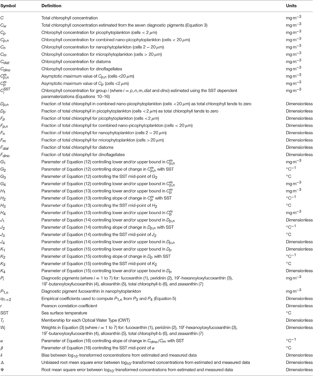
Table 1. Symbols and definitions.

2.3. Data

2.3.1. High Performance Liquid Chromatography (HPLC) Pigment Data

A total of 2,791 samples collected in the North Atlantic region and analyzed by High Performance Liquid Chromatography (HPLC) were used in this study (Figure 1), spanning 1995–2014. This dataset comprised of samples from: the Atlantic Meridional Transect (AMT) cruises 1-23 (Gibb et al., 2000; Barlow et al., 2002; Aiken et al., 2009; Brewin et al., 2010; Airs and Martinez-Vicente, 2014a,b,c; Brewin et al., 2015); the GeP&CO program (Dandonneau et al., 2004); the North Atlantic bloom experiment (Werdell et al., 2003; Westberry et al., 2010); the eastern Atlantic Ocean (Brotas et al., 2013); the North Atlantic, collected by the Bedford Institute of Oceanography (Sathyendranath et al., 2001; Devred et al., 2006); the Western Channel Observatory in the English Channel (Station L4 and E1; Smyth et al., 2010); a series of UK NERC-funded research cruises (D261, D262, D264, D325, JC011, JC037, and JCR656) in the North Atlantic and North Sea (Tilstone et al., 2015); and from the NASA bio-Optical Marine Algorithm Dataset (NOMAD Version 2.0 ALPHA, Werdell and Bailey, 2005), following the removal of any AMT data so as to avoid duplication. Details of HPLC methods used can be found in the aforementioned references.

Only samples collected within the top 20 m of the water column (or within the 1st optical depth as in the case of the NASA NOMAD dataset) were used [i.e., within the surface mixed-layer depth (rarely < 20 m; de Boyer Montégut et al., 2004)]. To control the quality of the pigment data, we used only HPLC data for which the total chlorophyll concentration was greater than 0.001 mg m⁻³ (Uitz et al., 2006), and the difference between the total chlorophyll concentration and the total accessory pigments was less than 30% of the total pigment concentration (Trees et al., 2000; Aiken et al., 2009; Brewin et al., 2015).

2.3.1.1. Size-fractionated chlorophyll estimates from HPLC

The fractions of total chlorophyll for the three phytoplankton size classes (F_p, F_n, and F_m, for pico-, nano-, and microplankton, respectively) were estimated following the methods of Brewin et al. (2015), adapted from Vidussi et al. (2001), Uitz et al. (2006), Brewin et al. (2010), and Devred et al. (2011). Note, whenever we refer to microplankton, nanoplankton and picoplankton, we are referring to phytoplankton. First, the total chlorophyll concentration (C) was estimated from the weighted sum of the seven diagnostic pigments, hereafter denoted C_w, according to

$C_w={\displaystyle \sum _{i=1}^7{W}_i}{P}_i,(3)$

where, the weights are denoted [W], and the diagnostic pigments [P] = {fucoxanthin; peridinin; 19′-hexanoyloxyfucoxanthin; 19′-butanoyloxyfucoxanthin; alloxanthin; total chlorophyll-b; zeaxanthin}. We computed the weights [W] using multi-linear regression on the 2,791 samples. Retrieved values for the weights compare reasonably to values derived globally (Table 2), and total chlorophyll (C) and total chlorophyll estimated from Equation (3) (C_w) were in good agreement (r = 0.99, Ψ = 0.10). Having derived C_w, the fractions of chlorophyll in each size class relative to the total chlorophyll concentration were estimated.

TABLE 2

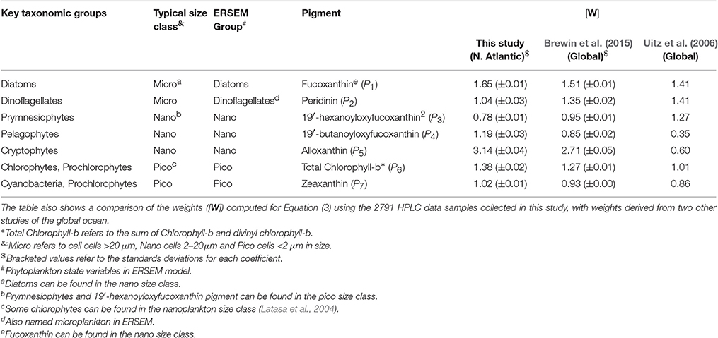
Table 2. Key taxonomic groups of phytoplankton, their typical size class, their category in the ERSEM model and their diagnostic pigment.

Following Brewin et al. (2015), the fraction of picoplankton chlorophyll concentration (F_p) was computed according to

$F_p=\{\begin{array}{ll}\frac{(-12.5C+1)W_3{P}_3}{C_w}+\frac{{\displaystyle {\sum }_{i=6}^7{W}_i{P}_i}}{C_w}\hfill & \text{if }C\le \text{0}.\text{08}\text{ mg}{\text{ m}}^{-3}\hfill \\ \frac{{\displaystyle {\sum }_{i=6}^7{W}_i{P}_i}}{C_w}\hfill & \text{if }C>\text{0}.\text{08}\text{ mg}{\text{ m}}^{-3}.\hfill \end{array}(4)$

The fraction of nanoplankton chlorophyll concentration (F_n) was estimated by first apportioning part of the fucoxanthin pigment (P₁) to the nanoplankton pool, as conducted by Devred et al. (2011), such that

$P_{1,n}={10}^{\{q_1{\log }_{10}(P_3)+q_2{\log }_{10}(P_4)\}},(5)$

where P₃ and P₄ refer to 19′-hexanoyloxyfucoxanthin and 19′-butanoyloxyfucoxanthin. This is to account for the fact that fucoxanthin is a precursor to 19′-hexanoyloxyfucoxanthin and 19′-butanoyloxyfucoxanthin (Devred et al., 2011). We recomputed these coefficients (q₁ and q₂) using the 2,791 HPLC samples, and arrived at values of q₁ = 0.14 and q₂ = 1.35. For any sample where P_1,n was higher than P₁, then P_1,n was set to equal P₁. Following Brewin et al. (2015), the fraction of nanoplankton chlorophyll concentration (F_n) was then estimated according to

$F_n=\{\begin{array}{ll}\frac{12.5C{W}_3{P}_3}{C_w}+\frac{{\displaystyle {\sum }_{i=4}^5{W}_i{P}_i+W_1{P}_{1,n}}}{C_w}\hfill & \text{if}C\le \text{0}.{08\text{ mg m}}^{-3}\hfill \\ \frac{{\displaystyle {\sum }_{i=3}^5{W}_i{P}_i+W_1{P}_{1,n}}}{C_w}\hfill & \text{if}C>0.{08\text{ mg m}}^{-3}.\hfill \end{array}(6)$

Finally, following Devred et al. (2011) and Brewin et al. (2015), the fraction of microplankton chlorophyll concentration (F_m) was estimated as

$F_m=\frac{{\displaystyle {\sum }_{i=1}^2{W}_i{P}_i-W_1{P}_{1,n}}}{C_w}.(7)$

Note that F_m can also be computed by simply subtracting F_n and F_p from one. The fractions of chlorophyll in each size class were then multiplied by the corresponding HPLC-derived total chlorophyll concentration (C) to derive the size-specific chlorophyll concentrations for each sample (C_p, C_p,n, C_n, and C_p, where the subscripts “p” refers to pico-, “n” nano- and “m” microphytoplankton, and the subscript “p,n” refers to combined pico and nanophytoplankton).

2.3.1.2. Partitioning the fraction of microphytoplankton chlorophyll into fractions of diatoms and dinoflagellates

The fraction of microphytoplankton chlorophyll concentration (F_m) is estimated from two diagnostic pigments, fucoxanthin in microphytoplankton (P_{1, m}) and peridinin (P₂). It is generally assumed that fucoxanthin in microphytoplankton is the primary pigment for diatoms (Stauber and Jeffrey, 1988) and peridinin for dinoflagellates, as the majority of photosynthetic dinoflagellates contain a chloroplast with peridinin as the major carotenoid (see Table 1 and Zapata et al., 2012). Following Hirata et al. (2011), this assumption was used to partition microphytoplankton chlorophyll into the concentrations of the two groups.

The fraction of microplankton diatoms to total chlorophyll (F_diat) and the fraction of microplankton dinoflagellates to total chlorophyll (F_dino) were computed as

$F_{diat}=\frac{W_1{P}_1-W_1{P}_{1,n}}{C_w},(8)$

and

$F_{dino}=\frac{W_2{P}_2}{C_w},(9)$

respectively. The chlorophyll concentrations for diatoms and dinoflagellates (C_diat and C_dino) were then obtained by multiplying the fractions by the corresponding HPLC-derived total chlorophyll concentration (C).

2.3.2. Size-Fractionated Filtration (SFF) Data

A total of 263 size-fractionated fluorometric chlorophyll (SFF) measurements collected previously in the North Atlantic region were also used in this study (Figure 1), spanning 1996–2015. This comprised of samples from: the Atlantic Meridional Transect cruises 2–23 (see Marañón et al., 2001; Serret et al., 2001; Robinson et al., 2002; Brewin et al., 2014a,b; Tilstone et al., 2017, for details); the Western Channel Observatory in the English Channel (Station L4 and E1; see Barnes et al., 2014, for details); and the NERC shelf seas biogeochemistry programme.

In all cases, ~200–300 ml samples were sequentially filtered through 20, 2, and 0.2 μm polycarbonate filters. Following filtration, pigments were extracted by storing the filters in 90% acetone at −20°C for between 10 and 24 h. Samples were then analyzed using a Turner Design Fluorometer, pre- and post-calibrated using pure chlorophyll-a in 90% acetone as a standard. The total chlorophyll concentration was taken as the sum of the size fractions for each sample. The concentration of chlorophyll passing through the 2 μm filter was designated C_p (picoplankton chlorophyll), chlorophyll retained on the 20 μm filter designated C_m (microplankton chlorophyll) and the chlorophyll retained on the 2 μm filter, having passed through the 20 μm filter, designated C_n (nanoplankton chlorophyll).

2.4. Merging of in situ Datasets

Systematic biases in size-fractionated chlorophyll estimated from HPLC pigments and from SFF have been observed in the Atlantic Ocean (Brewin et al., 2014a), with implications for models that estimate size-fractionated chlorophyll as a function of total chlorophyll (Brewin et al., 2014b) and models that estimate size-fractionated primary production (Brewin et al., 2017). Therefore, care needs to be taken when combining these two datasets. Figure 2 shows a comparison of 31 concurrent and co-located data points of total chlorophyll (Figure 2A), picoplankton chlorophyll (Figure 2B), nanoplankton chlorophyll (Figure 2C) and microplankton chlorophyll (Figure 2D), from the HPLC and SFF dataset used here.

FIGURE 2

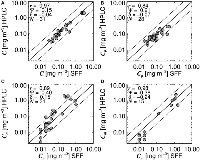
Figure 2. Concurrent and co-located size-fractionated chlorophyll estimated from High Performance Liquid Chromatography (HPLC) and size-fractionated filtration (SFF) for surface waters in the North Atlantic region. (A) shows a comparison of total chlorophyll (C), (B) picoplankton chlorophyll (C_p), (C) nanoplankton chlorophyll (C_n), and (D) microplankton chlorophyll (C_m). Black line represents the 1:1 line and dotted lines represent the 1:1 line ±30% log₁₀ chlorophyll. N refers to the number of samples used to compute statistics, r refers to the Pearson linear correlation coefficient, Ψ the root mean square error (Equation 1) and δ the bias (Equation 2).

Despite there being biases in size-fractionated chlorophyll consistent with those observed by Brewin et al. (2014a) (Figure 2), these biases are notably smaller (e.g., for picoplankton chlorophyll δ = −0.07 compared with δ = −0.27 in see their Figure 3 Brewin et al. (2014a), and for nanoplankton δ = 0.15 compared with δ = 0.22), suggesting for surface waters in the North Atlantic, there is reasonable agreement between the two methods, at least for the datasets used here. Given the good agreement in Figure 2, the two datasets were combined into a single dataset, providing 3,054 measurements of size-fractionated chlorophyll (2,791 HPLC and 263 SFF). Figure 3 shows a schematic diagram of how the datasets were combined and subsequently used for model parameterization and validation.

FIGURE 3

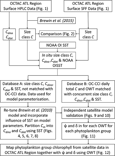
Figure 3. A flow chart of the processing techniques. Data collected in the OCTAC ATL region [both High Performance Liquid Chromatography (HPLC) and size-fractionated filtration (SFF)] were partitioned into two databases [parameterization (Database A) and satellite validation (Database B)], and used to re-tune, adapt and validate the model of Brewin et al. (2010), compute the root mean square error (Ψ) and bias (δ) for each optical water type (OWT), and map phytoplankton group products and associated errors using ocean-color data.

For each sample, SST data were extracted by matching each in situ sample in time (daily temporal match-up) and space (closest latitude and longitude) with daily, 1/4° resolution Optimal Interpolation Sea Surface Temperature (OISST) data (Version 2.0; Reynolds et al., 2007) acquired from the NOAA website (http://www.esrl.noaa.gov/psd/data/gridded/data.noaa.oisst.v2.highres.html).

2.5. Partitioning Into Parameterization and Validation Datasets

The merged dataset was matched to daily, level 3 (4 km sinusoidal projected) satellite chlorophyll and optical water type (OWT) data, from version 3.0 of the Ocean Colour Climate Change Initiative (OC-CCI, a merged MERIS, MODIS-Aqua, SeaWiFS and VIIRS product available at http://www.oceancolour.org/), between 1997 and 2015. Each in situ sample was matched with a single satellite pixel in time (daily match-up) and space (closest pixel with a distance < 4 km away). Of the 3,054 samples, there were 815 corresponding satellite chlorophyll and optical water type (OWT) data. These 815 measurements were set aside and used for independent validation of the satellite model and for characterizing per-pixel error, leaving 2,239 measurements that were used for model development (parameterization). Figure 3 shows a schematic diagram of how the data were partitioned into the parameterization and validation dataset.

The OWT data provided in version 3.0 of the OC-CCI dataset contains the per-pixel membership of 14 different optical classes, ranging from oligotrophic (e.g., OWT 1) to very turbid (OWT 14) waters. Building on the work of Moore et al. (2001, 2009, 2012), this new set of optical classes were constructed for use with OC-CCI remote sensing reflectance (R_rs) spectra (Jackson and Sathyendranath, 2015). These classes were trained using R_rs spectra from satellite data, rather than using a database of in situ observations, as conducted in Moore et al. (2009), and the number of optical water classes were increased to 14, to better cover the range of R_rs spectra observed in the global oceans, particularly the oligotrophic gyres. For further details of the training and production of the 14 OWT the reader is referred to Jackson and Sathyendranath (2015).

2.6. Satellite Model of Phytoplankton Groups

2.6.1. Three-Component Model of Brewin et al. (2010)

As a starting point, we used the three-component model of Brewin et al. (2010) to estimate the chlorophyll concentrations in three phytoplankton size classes [pico- (< 2 μm), nano- (2–20 μm), and micro-phytoplankton (>20 μm)] as a function of total chlorophyll in the study region (Figure 1). This approach has been successfully tuned to the global ocean (Brewin et al., 2015; Ward, 2015) as well as different oceanic regions, including: the Atlantic Ocean (North and South; Brewin et al., 2010, 2014b; Tilstone et al., 2014); the North East Atlantic (Brotas et al., 2013); the Indian Ocean (Brewin et al., 2012b); the Western Iberian coastline (Brito et al., 2015); the Mediterranean Sea (Sammartino et al., 2015); and the South China Sea (Lin et al., 2014). Estimating size-fractionated chlorophyll from satellite data (using satellite total chlorophyll as input to the three-component model) has been tested extensively with in situ data in different oceanic regions (Brewin et al., 2010, 2012b; Lin et al., 2014; Brewin et al., 2015).

The three-component model is based on two exponential functions (Sathyendranath et al., 2001), where the chlorophyll concentration of picoplankton (C_p, cells < 2 μm) and combined pico- and nanoplankton (C_p,n, cells < 20 μm) are obtained from

$C_{p,n}=C_{p,n}^m[1-\exp (-\frac{D_{p,n}}{C_{p,n}^m}C)],(10)$

and

$C_p=C_p^m[1-\exp (-\frac{D_p}{C_p^m}C)].(11)$

The parameters D_p,n and D_p determine the fraction of total chlorophyll in the two size classes (< 20 μm and < 2 μm, respectively) as total chlorophyll tends to zero, and $C_{p,n}^m$ and $C_p^m$ are the asymptotic maximum values for the two size classes (< 20 μm and < 2 μm respectively). The chlorophyll concentration of nano-phytoplankton (C_n) and micro-phytoplankton (C_m) are simply calculated as C_n = C_p,n − C_p and C_m = C − C_p,n.

A single set of model parameters was first derived by fitting (Equations 10 and 11) using a standard, nonlinear least-squared fitting procedure (Levenberg-Marquardt, IDL Routine MPFITFUN, Moré, 1978; Markwardt, 2008) with relative weighting (Brewin et al., 2011a). The parameters D_p,n and D_p were constrained to be less than or equal to one, since size-fractionated chlorophyll cannot exceed total chlorophyll. We used the method of bootstrapping (Efron, 1979; Brewin et al., 2015) to compute a parameter distribution, and from the resulting parameter distribution, median values and 95% confidence intervals were computed (see Table 3). The parameters D_p,n and D_p were found to be significantly different from the global parameters derived in Brewin et al. (2015) (see Table 3). The model was found to capture the trends in the fractions (F_p, F_n, F_p,n, and F_m) and absolute concentrations (C_p, C_n, C_p,n, and C_m) of the size classes as a function of total chlorophyll for the North Atlantic parameterization dataset (Figure 4).

TABLE 3

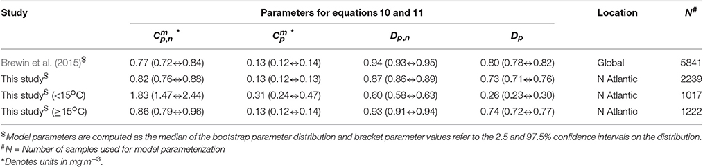
Table 3. Parameter values for Equations 10 and 11 compared with global parameters derived in Brewin et al. (2015).

FIGURE 4

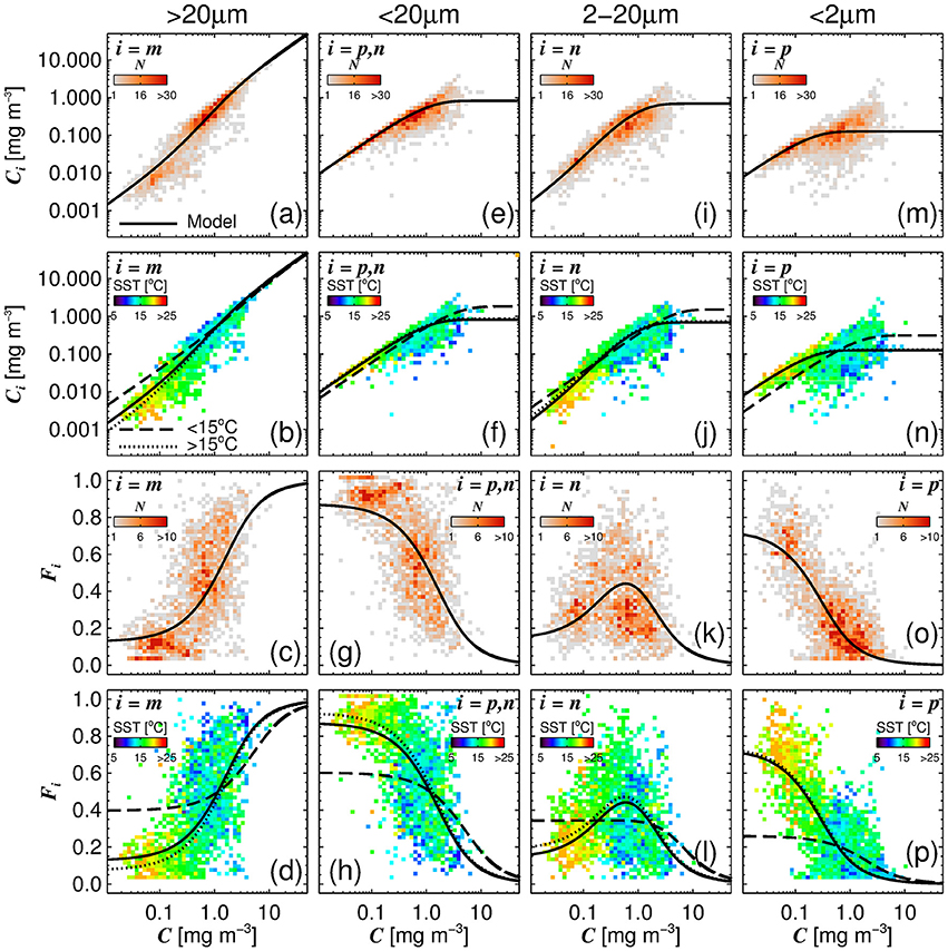
Figure 4. The absolute chlorophyll concentrations [C_m (a,b), C_p,n (e,f), C_n (i,j), and C_p (m,n)] and fractions [F_m (c,d), F_p,n (g,h), F_n (k,l) and F_p (o,p)] in the parameterization dataset plotted as a function of total chlorophyll concentration (C), with the re-tuned (Brewin et al., 2010) model (parameters from Table 3), overlain. The top row (a,e,i,m) and middle-bottom row (c,g,k,o) show bivariate histogram plots with the shading indicating the number of observations (N). The bottom row (d,h,l,p) and middle-top row (b,f,j,n) show the same bivariate plots but the shading represents the median sea surface temperature (SST) of the data points that lie within the bins.

2.6.2. Modification of Three-Component Model Using SST

Brewin et al. (2015) and Ward (2015) have investigated the influence of light availability and SST respectively on the parameterization of the three-component model. In the North Atlantic, seasonal variations in SST and the average light in the mixed-layer are highly correlated (Figure 1). Therefore, considering: (i) that there is, regionally, a covariation of SST with the average light in the mixed-layer (Figure 1); (ii) that three inputs are required to compute the average light in the mixed-layer (photosynthetically-active radiation, diffuse attenuation and mixed-layer depth), one of which is not amenable from remote-sensing (mixed-layer depth); and (iii) that the maturity (operational use) and accuracy of SST retrievals is very high (Merchant et al., 2014), we chose to investigate the influence of SST on model parameters in the study area, similar to the study of Ward (2015) for a global dataset.

Figure 4 illustrates the general inverse correlation between SST and total chlorophyll (r = −0.67 for SST and log₁₀(C)), highlighting that higher fractions of smaller cells (lower fractions of large cells) are typically associated with higher SST. To investigate if SST has any influence on the parameters of the three-component model, we partitioned the parameterization data into lower temperature waters (< 15°C) and higher temperature waters (≥15°C), and fitted the model separately to the two datasets of a roughly equal number (>1,000, see Table 3). We observed significantly different model parameters for high and low temperature waters (see Table 3 and Figure 4), suggesting a relationship between SST and model parameters. We then sorted the dataset according to SST, and conducted a running fit of the three-component model (Equations 10 and 11) as a function of SST with a bin size of 600 samples [chosen to ensure each fit had reasonable representation of observations over the entire trophic range (low to high chlorophyll)]. We used the method of bootstrapping (100 iterations) and derived median values and 95% confidence intervals on each parameter distribution (Figure 5).

FIGURE 5

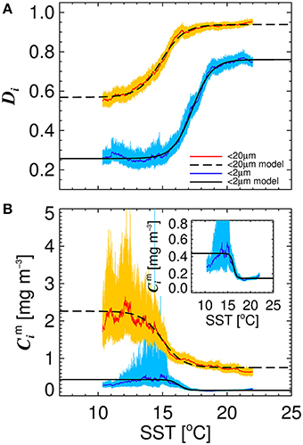
Figure 5. The relationship between sea surface temperature (SST) and the parameters of the re-tuned (Brewin et al., 2010) model for the North Atlantic dataset. (A) Shows the relationship between D_p,n and SST, and D_p and SST. (B) Shows the relationship between $C_{p,n}^m$ and SST, and $C_p^m$ and SST. Solid color lines show median values on the bootstrap parameter distribution and lighter shades represent 95% confidence intervals. Black solid and dashed lines represent logistic models fitted between the parameters and SST shown in Equations (12–15), with the parameters provided in Table 4.

Significant relationships between all model parameters ($C_{p,n}^m$, $C_p^m$, D_p,n, and D_p) and SST were observed (Figure 5). The relationship between SST and model parameters could be represented using a logistic function, such that $C_{p,n}^m$ and $C_p^m$ may be expressed as

$C_{p,n}^m=1-\{\frac{G_1}{1+\exp [-G_2(\text{SST}-G_3)]}+G_4\},(12)$

and

$C_p^m=1-\{\frac{H_1}{1+\exp [-H_2(\text{SST}-H_3)]}+H_4\},(13)$

where G₁ and G₄ control the upper and lower bounds of $C_{p,n}^m$, G₂ represents the slope of change in $C_{p,n}^m$ with SST, and G₃ is the SST mid-point of the slope between $C_{p,n}^m$ and SST. For $C_p^m$, H_i, where i = 1–4, is analogous to G_i for $C_{p,n}^m$. The parameter D_p,n and D_p were expressed as

$D_{p,n}=\frac{J_1}{1+\exp [-J_2(\text{SST}-J_3)]}+J_4,(14)$

and

$D_p=\frac{K_1}{1+\exp [-K_2(\text{SST}-K_3)]}+K_4,(15)$

where J₁ and J₄ control the upper and lower bounds of D_p,n, J₂ represents the slope of change in D_p,n with SST, and J₃ is the SST mid-point of the slope between D_p,n and SST. For D_p, K_i is analogous to J_i for D_p,n. The parameters for Equations (12)–(15) were fitted using a nonlinear least-squared fitting procedure (Levenberg-Marquardt) with bootstrapping, and parameter values are provided in Table 4. The equations are seen to capture the relationships between parameters and SST accurately (Figure 5 and Table 4).

TABLE 4

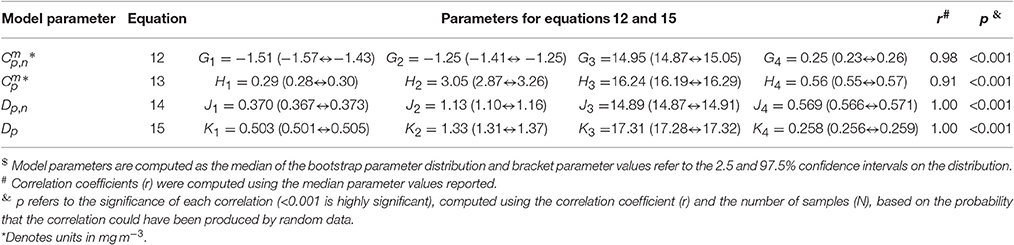
Table 4. Parameter values for Equations (12) and (15).

Figure 6 shows simulations of size-fractionated chlorophyll as a function of total chlorophyll for different SST, when incorporating (Equations 12–15) into the three-component model (Equations 10 and 11). In general, the performance for all size classes improved when using the SST-dependent parameterization, when compared with that using a single set of parameters (Figure 7), with a significant improvement in the correlation coefficient for C_p (Z-test, p < 0.05). Whereas modeled C_p,n, C_n, and C_p reach static asymptotes at high concentrations when using a single set of parameters (see Figure 7, top-row, horizontal purple dashed lines), the SST-dependent parameterization does not, and captures the variability in the size-fractionated chlorophyll at these higher concentrations.

FIGURE 6

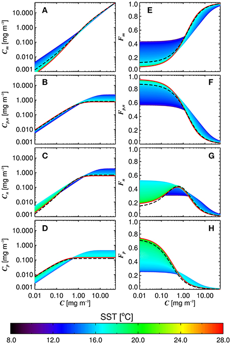
Figure 6. Size-fractionated chlorophyll (A–D) and the fractions of total chlorophyll in each size class (E–H) plotted as a function of the total chlorophyll using the re-tuned (Brewin et al., 2010) model, and varying the parameters according to the sea surface temperature (SST) (Equations 12–15). Dashed black lines refer to the re-tuned model using a single set of parameters (Table 3).

FIGURE 7

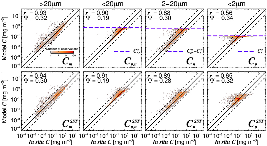
Figure 7. The modeled size-fractionated chlorophyll plotted against in situ size-fractionated chlorophyll in the parameterization dataset, for the re-tuned (Brewin et al., 2010) model with a single set of parameters (top-row, Table 3) and using the SST-dependent parameterization (bottom row, Equations 12–15, Table 4). The superscript SST denotes the modeled chlorophyll concentrations using the SST-dependent parameterization. The correlation coefficient (r) and root-mean-square-error (Ψ) are also shown. Statistical tests were computed using the parameter values reported in Tables 3, 4. The top panels also show the maximum attainable concentrations for the different size classes as purple dashed horizontal lines when using a single set of parameters (Table 3).

2.6.3. Partitioning of Microphytoplankton Chlorophyll Into Diatoms and Dinoflagellates

Considering diatoms are known to dominate the microphytoplankton community in the North Atlantic during the initiation of the spring bloom when SST is still relatively low and nutrient concentrations high (Ducklow and Harris, 1993; Sieracki et al., 1993; Savidge et al., 1995), and that dinoflagellates typically increase in late summer and early autumn (McQuatters-Gollop et al., 2007; Widdicombe et al., 2010) when SST is generally at its highest in the North Atlantic, we investigated the use of SST to partition microplankton chlorophyll (C_m) into diatoms (C_diat) and dinoflagellates (C_dino). Figure 8A shows a significant relationship between ratio of C_dino to C_m and SST (r = 0.28, p < 0.001), with the ratio increasing with increasing SST. We modeled this relationship by fitting a logistic function to the data (Figure 8A), such that

$\frac{C_{dino}}{C_m}=\frac{1}{1+\exp [-\alpha (\text{SST}-\beta )]},(16)$

where α = 0.10 (0.08↔0.13) and β = 32.5 (29.7↔36.1). Figures 8B,C show model estimates of C_dino (obtained by multiplying the modeled ratio (Equation 16) by C_m) plotted against measured C_dino, and estimates of C_diat (obtained as C_m(1−(C_dino/C_m))) against measured C_diat. In general, there is good agreement between the estimates and measurements, with higher correlations and lower root mean square errors for C_diat compared with C_dino (Figures 8B,C). Combining estimates of C_m using the three component model (Equations 10–15) with estimates of the ratio of C_dino to C_m (Equation 16), C_dino and C_diat can be estimated as a function of total chlorophyll (C) and SST.

FIGURE 8

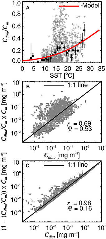
Figure 8. (A) The ratio of dinoflagellate chlorophyll (C_dino) to microplankton chlorophyll (C_m) plotted as a function of sea surface temperature (SST). Gray points show raw values, black dots are binned averages with 95% confidence intervals on the averages, and red line show the fitted model (Equation 16). (B) Shows the modeled ratio (Equation 16) multiplied by microplankton chlorophyll (C_m) to estimate C_dino, plotted against measured C_dino. (C) Shows one minus the modeled ratio (Equation 16) multiplied by microplankton chlorophyll (C_m) to estimate C_diat, plotted against measured C_diat. r is the correlation coefficient and Ψ the root-mean-square-error.

2.7. Validation of the Satellite Model, Estimates of Per-Pixel Uncertainty and Application to Satellite Data

The satellite match-up dataset (not used for model parameterization) was used to validate the model by using satellite-derived total chlorophyll (OC-CCI) and SST (NOAA OISST) as inputs to Equations (10–15) and comparing the results with independent in situ chlorophyll concentrations for each phytoplankton group. In addition, the satellite match-ups were partitioned into 14 OWT by selecting the highest OWT membership for each sample. The root mean square error (Ψ, Equation 1) and bias (δ, Equation 2) in the satellite estimates were computed separately for each OWT and for each phytoplankton group.

We applied the model to a relatively cloud-free 8-day chlorophyll (OC-CCI) and SST (NOAA OISST) composite for the data between 17th and 24th June 2008, to illustrate its application to a satellite image. Uncertainties (Ψ and δ) in each pixel of the study area were computed by weighing the uncertainties in each OWT by their membership. For instance, Ψ at a given pixel for a hypothetical phytoplankton group would be computed as

$\Psi =\frac{{\displaystyle {\sum }_{i=1}^{14}{\Psi }_i{T}_i}}{{\displaystyle {\sum }_{i=1}^{14}{T}_i}},(17)$

where i represents each OWT and T represents the membership of each OWT.

3. Results and Discussion

3.1. Satellite Validation

Considering the agreement between total satellite and in situ chlorophyll in the validation dataset (r = 0.86, Ψ = 0.29, δ = −0.01), the satellite estimates of size-fractionated chlorophyll compare well with the independent in situ data (Figure 9, r = 0.49 to 0.86, and Ψ = 0.30 to 0.45), in agreement with previous studies (Brewin et al., 2010, 2012b; Lin et al., 2014; Brewin et al., 2015). Although the SST-dependent parameterization ($C_i^{SST}$) has a similar statistical performance compared with that obtained when using a single set of parameters, the SST-dependent parameterization is not constrained by static asymptotes for C_p,n, C_n, and C_p (Figure 9 top-row, horizontal purple dashed lines) and captures better the variability in the size-fractionated chlorophyll at these higher concentrations. Correlation coefficients for picoplankton chlorophyll are higher for the SST-dependent parameterization ($C_p^{SST}$) when compared with the single set of parameters (C_p) in both the parameterization (Figure 7) and validation (Figure 9) datasets. This finding is consistent with results from Pan et al. (2013) who highlighted the benefits of including SST when estimating zeaxanthin (diagnostic pigment for picoplankton) from satellite data.

FIGURE 9

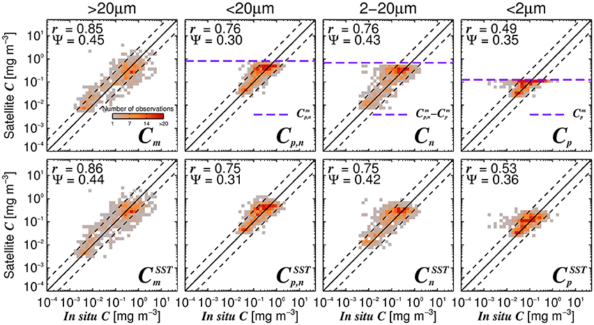
Figure 9. Satellite estimates of size-fractionated chlorophyll plotted against independent in situ size-fractionated chlorophyll in the validation dataset, for the re-tuned (Brewin et al., 2010) model with a single set of parameters (top-row, Table 3) and using the SST-dependent parameterization (bottom row, Equations 12–15). The superscript SST denotes the modeled chlorophyll concentrations using the SST-dependent parameterization. The correlation coefficient (r) and root-mean-square-error (Ψ) are also shown. Statistical tests were computed using the parameter values reported in Tables 3, 4. The top panels also show the maximum attainable concentrations for the different size classes as purple dashed horizontal lines when using a single set of parameters (Table 3).

Satellite estimates of diatom and dinoflagellate chlorophyll also compare reasonably well with the independent in situ data (Figure 10). Satellite estimates of diatom chlorophyll have higher correlation coefficient (r) and lower error (Ψ) when compared with dinoflagellate chlorophyll estimates, suggesting better performance for this phytoplankton group. High errors in satellite estimates of dinoflagellate chlorophyll reflect how challenging it is to retrieve this phytoplankton group from space (Raitsos et al., 2008; Shang et al., 2014), though it is encouraging to observe significant correlations between the satellite and in situ dinoflagellate chlorophyll concentrations (r > 0.64, p < 0.001) in the validation dataset, especially when considering the lower range of chlorophyll variability in dinoflagellates (Figure 10).

FIGURE 10

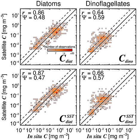
Figure 10. Satellite estimates of diatom (C_diat) and dinoflagellate (C_dino) chlorophyll plotted against independent in situ estimates of C_diat and C_dino in the validation dataset, using the Brewin et al. (2010) model with a single set of parameters (top-row, Table 3) together with estimates of C_dino/C_m (Equation 16), and using the SST-dependent parameterization (bottom row, Equations 12–15) together with estimates of C_dino/C_m (Equation 16). The superscript SST denotes the modeled microplankton chlorophyll using the SST-dependent parameterization (Equations 12–15) multiplied by estimates of C_dino/C_m (Equation 16). The correlation coefficient (r) and root-mean-square-error (Ψ) are also shown.

3.2. Changes in Performance With Optical Water Types (OWT)

For each of the 14 OWT and for each of the phytoplankton groups, the root mean square error (Ψ), bias (δ) and number of observations (N) for match-ups in the validation dataset are provided in Table 5. The Ψ, δ, and N are also plotted in Figure 11 for satellite estimates of total chlorophyll and chlorophyll for the four phytoplankton groups using the SST-dependent parameterization (Equations 12 to 15). The Ψ values in each OWT for total chlorophyll are consistent with those provided in version 3.0 of the OC-CCI dataset, based on a much larger global match-up dataset (~14,500) (Figure 11A). The Ψ values for total chlorophyll increase from lower OWTs (characteristic of oligotrophic open-ocean waters) to higher OWTs (characteristic of more optically complex turbid coastal waters). A result that is also consistent with the original work of Moore et al. (2009), see their Table 2, and the theoretical limitations of using empirical ocean-color chlorophyll algorithms in optically-complex waters (IOCCG, 2000). Biases (δ) in total chlorophyll are generally quite low (Figure 11B), consistent with version 3.0 of the OC-CCI dataset, though do not always have the same sign, and are much higher for OWT14, probably due to very few match-ups (N = 4) in this class (Figure 11B).

TABLE 5

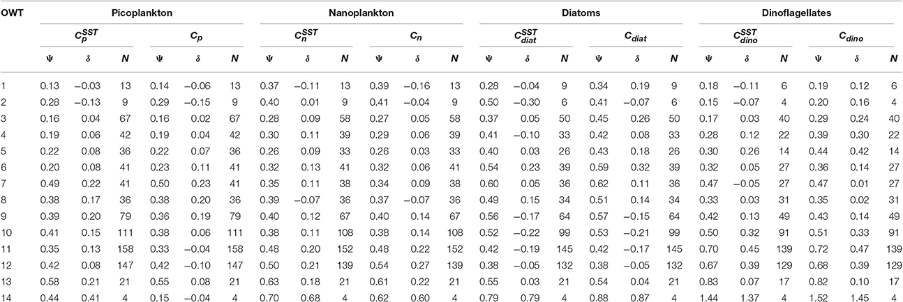
Table 5. Root mean square error (Ψ) and bias (δ) for 14 OC-CCI optical water types (OWT) for the four phytoplankton groups, using the two approaches (SST-dependent with superscript SST, and single set of parameters) to estimate phytoplankton group chlorophyll from satellite data.

FIGURE 11

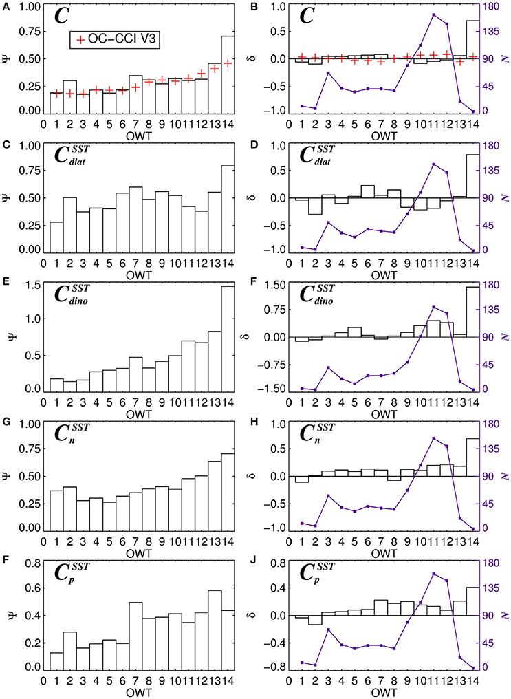
Figure 11. The average root-mean-square-error (Ψ) and bias (Ψ) for 14 dominant OC-CCI Optical Water Types (OWT) for total chlorophyll (A,B), diatom chlorophyll (C,D), dinoflagellate chlorophyll (E,F), nanoplankton chlorophyll (G,H), and picoplankton chlorophyll (I,J). N (violet lines and squares) shows the number of observations of each dominant OWT. Plots (C–J) are for the SST-dependent parameterization (Equations 12–15) together with estimates of C_dino/C_m (Equation 16).

Consistent with satellite estimates of total chlorophyll, there is a tendency for Ψ to increase from lower to higher OWTs for all the phytoplankton groups (Table 5, Figures 11C,E,G,I), particularly for smaller cells (pico and nano-plankton) and for dinoflagellates. This is likely due to: i) the satellite estimates of total chlorophyll, which are used as input to the phytoplankton group model, having larger errors at higher OWTs (Figure 11A); and ii) possible deviations in the relationships between the phytoplankton groups and total chlorophyll in optically complex waters, when compared with typical open-ocean conditions. With the exception of diatoms, there is a slight tendency for the models to overestimate chlorophyll for the phytoplankton groups at higher OWTs (e.g., 8–14), as indexed by a positive bias (Table 5, Figures 11F,H,J).

3.3. Application of the Model to a Satellite Image

Figure 12 illustrates the application of the phytoplankton group model (SST-dependent parameterization; Equations 10–15) to satellite chlorophyll (OC-CCI) and SST (NOAA OISST) composites for the period 17th to 24th June 2008. Satellite products used as inputs to the model – chlorophyll (Figure 12A), OWT membership (plotted by dominance (highest membership) in Figure 12B) and SST (Figure 12C)—highlight the different biogeochemical areas in the region, with oligotrophic waters to the south (high SST, low total chlorophyll, low OWT), more productive waters to the north (lower SST, higher chlorophyll and OWT), and very productive coastal waters (variable SST, high chlorophyll and OWT). Figures 12D,G,J,M, show estimates of chlorophyll for the four phytoplankton groups, diatoms (C_diat), dinoflagellates (C_dino), nanoplankton (C_n) and picoplankton (C_p), respectively. Picoplankton (C_p) are the dominant group in the warm oligotrophic waters, nanoplankton (C_n) in intermediate (mesotrophic waters), and diatoms (C_diat) in the northern productive waters and coastal regions (eutrophic waters). Dinoflagellates rarely dominate (i.e., rarely have the highest chlorophyll of the four groups), but typically have higher concentrations in coastal regions.

FIGURE 12

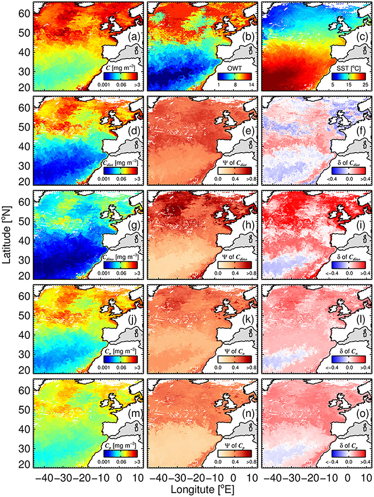
Figure 12. Satellite estimates of phytoplankton group chlorophyll and per-pixel errors for an 8 day (relatively clear sky) composite (17th to 24th June 2008) of OC-CCI chlorophyll (a), (dominant) optical water type (b) and SST (NOAA OISST) data (c). Example shown is using the SST-dependent parameterization (Equations 12–15) together with estimates of C_dino/C_m (Equation 16): (d) Diatom chlorophyll (C_diat); (e) per-pixel root-mean-square-error (Ψ) of C_diat; (f) per-pixel bias (δ) of C_diat; (g) dinoflagellate chlorophyll (C_dino); (h) Ψ of C_dino; (i) δ of C_dino; (J) nanoplankton chlorophyll (C_n); (k) Ψ of C_n; (l) δ of C_n; (m) picoplankton chlorophyll (C_p); (n) Ψ of C_p; and (o) δ of C_p.

In addition to the concentrations, per-pixel uncertainties (Ψ and δ) are plotted for each phytoplankton group (Figure 12), through application of Equation (17) on a per-pixel basis, using per-pixel OWT membership provided by the OC-CCI products and statistics from Table 5. In general, lower Ψ is observed in the oligotrophic waters to the south of the region, with Ψ increasing toward more productive waters. Dinoflagellates have the highest Ψ in these productive waters, reflecting higher uncertainty in deriving the concentrations of this phytoplankton group (see also Figure 10). Lower Ψ are seen for nano- and picoplankton, when compared with the larger size classes. Diatoms display a less variable Ψ throughout the entire region, when compared with the other three phytoplankton groups.

Biases (δ) are close to zero for all phytoplankton groups in the warm oligotrophic waters (Figure 12), with positive biases seen for dinoflagellates, nanoplankton and picoplankton in the more productive waters, implying a slight overestimation in chlorophyll by the satellite model in these waters. These biases can be caused by two reasons: (i) biases in model input (total chlorophyll); and (ii) biases in model parameters used for partitioning total chlorophyll into the phytoplankton groups. There were no major biases (with the exception of OWT14) in total chlorophyll (model input) in the validation dataset (Figure 11B). Nonetheless, it is likely that the use of alternative input chlorophyll algorithms (e.g., a semi-analytical algorithm) will impact these biases. The positive biases seen for dinoflagellates, nanoplankton and picoplankton in the more productive waters are likely caused by biases in model parameters at higher OWTs. In the future, with a larger database, modifications to model parameters according to OWT could be feasible, and would likely reduce observed biases.

As well as varying within the region as illustrated in Figure 12, temporal variations in chlorophyll concentration and associated per-pixel errors can be captured by application of the model to satellite data over the course of the seasons.

3.4. Potential Caveats In the Approach

3.4.1. In situ Estimates of Phytoplankton Group Chlorophyll

The performance of a model is tightly related to the quality of data used to tune it. We used estimates of phytoplankton group chlorophyll principally from HPLC. Whereas recent refinements in the use of HPLC to infer size-fractionated chlorophyll (Uitz et al., 2006; Brewin et al., 2010; Devred et al., 2011; Brewin et al., 2015) were used, diagnostic pigments determined by HPLC can be found in a variety of phytoplankton taxa and size classes, such that its use as a single in situ method may not always be dependable (Nair et al., 2008). Therefore, we combined data on size-fractionated chlorophyll estimated from HPLC with those from SFF, which encouragingly, were found to be in reasonable agreement with each other for surface waters in the North Atlantic region (Figure 2). Yet, biases between the two techniques have been observed in Atlantic waters (Brewin et al., 2014a). Uncertainties in the SFF technique can arise from filter clogging, inaccurate pore sizes and cell breakage. The partitioning of microplankton chlorophyll into diatoms and dinoflagellates was based on the assumption that fucoxanthin in microphytoplankton can be attributed to diatoms and peridinin to dinoflagellates (Equations 8 and 9). Yet, there can also be fucoxanthin-containing dinoflagellates (e.g., Kryptoperidinium foliaceum) in Atlantic waters (Kempton et al., 2002), though there occurrence is generally not well known. Greater efforts to combine other sources of in situ data (e.g., flow cytometry, video imagery, optical measurements and microscopy) should help improve, and quantify uncertainty in, estimates of phytoplankton group chlorophyll in situ and ultimately, the parameterization of satellite models.

3.4.2. The Satellite Phytoplankton Group Model

The conceptual framework of the Brewin et al. (2010) model has been supported by data from: phytoplankton spectral absorption measurements (Brewin et al., 2011a); spectral particle backscattering measurements (Brewin et al., 2012a); chlorophyll estimated by size-fractionated filtration (Raimbault et al., 1988; Chisholm, 1992; Riegman et al., 1993; Gin et al., 2000; Marañón et al., 2012; Brewin et al., 2014a; Ward, 2015); flow cytometry and microscopy (Brotas et al., 2013). The model has also been found to reproduce inter-annual variations in size structure consistent with theories on coupling between physical-chemical processes and ecosystem structure (Brewin et al., 2012b), and found to reproduce the typical normalized-biomass size-spectrum of phytoplankton (Brewin et al., 2014b). The model has captured relationships between size structure and total chlorophyll in a variety of contrasting regions (e.g., Lin et al., 2014; Brito et al., 2015; Sammartino et al., 2015).

Yet, as with any abundance-based method, the model does not directly detect the phytoplankton groups: it simply infers the concentrations of chlorophyll in each group based on relationships, developed using data collected in the past, with properties that can by derived accurately from space (e.g., chlorophyll concentration and sea surface temperature). The model is not expected to capture blooms that deviate from the general trends observed in the parameterization dataset (Figures 4,5). For this reason, such techniques may not be appropriate for certain applications. For instance, under a climate-change scenario, there is the possibility that the relationships between properties (e.g., total chlorophyll and group-specific chlorophyll) may change, which may not be detected using an abundance-based approach (Sathyendranath et al., submitted). For such applications, spectral-based methods are likely to be preferable.

Two versions of the re-tuned Brewin et al. (2010) model were carried forward in this study: one using a fixed set of parameters (Table 3); and the other where the parameters were tied with SST (Table 4). The Brewin et al. (2010) model with a fixed parameter set has an advantage that only four parameters are required to compute the size fractions (Table 3), compared with 16 that are used in the SST-dependent model (Table 4). A larger dataset is required to tune the SST-dependent model for regional applications, when compared with the model with a fixed parameter set. Furthermore, when considering all samples together, only a slight improvement in model performance (Ψ and δ) was achieved when using the SST-dependent model (Figures 7, 9). Yet, the SST-dependent model captured variations in model parameters, such as the asymptotic maximum values for small cells ($C_{p,n}^m$ and $C_p^m$), that are known to vary with changes in bottom-up (e.g., nutrients and light) and top-down (grazing) processes (Riegman et al., 1993; Brewin et al., 2014b). The fixed parameter model simply failed to capture these variations, resulting in unrealistic static asymptotes (Figures 7, 9 top-row, horizontal purple dashed lines).

Variations in the relationships of size structure with total chlorophyll and with SST were generally consistent with those proposed by Ward (2015), with the fractions of larger cells (e.g., microplankton) generally increasing with decreasing SST, for concentrations of total chlorophyll less than 1 mg m⁻³, and the fractions of small cells (picoplankton) increasing (Figure 6). Yet, in the Ward (2015) study these variations were typically observed at lower temperature (< 5°C) than those shown in this study (< 17°C). Results are also relatively consistent for small cells (picoplankton) with those proposed by Brewin et al. (2015), when using average light in the mixed-layer, rather than SST, to vary model parameters, though differ for microplankton (see Figures 4, 5 of Brewin et al., 2015). Differences between studies are possibly due to the regional-tuning of the model when compared with the global studies of Ward (2015) and Brewin et al. (2015). There are also differences in the two approaches: whereas Ward (2015) introduces an additional term to the three-component model to account for temperature dependence, here we have let the model parameters change in response to SST variation.

Motivated by the need to provide satellite products of phytoplankton groups that match those as defined in ecosystem models, particularly ERSEM (Table 2), we proposed a partitioning of microplankton chlorophyll (C_m) into diatoms (C_diat) and dinoflagellates (C_dino), by modeling the ratio of C_dino to C_m as a function of SST (Figure 8A). This differs to that proposed by Hirata et al. (2011) which is based solely on total chlorophyll. We observed a significant relationship between C_dino/C_m and SST that was consistent with known seasonal variations of the two phytoplankton groups in the region (McQuatters-Gollop et al., 2007; Widdicombe et al., 2010). Yet, there still are significant variations surrounding this relationship (Figure 8A), and C_dino was found to have the highest errors in the satellite model (Figures 11, 12). The approach may fail to capture blooms of microplankton chlorophyll (C_m) entirely dominated by dinoflagellates (Figure 8A), that can occur in the region (Widdicombe et al., 2010). Future improvements in C_dino satellite estimates may be possible by incorporating spectral information (Shang et al., 2014) or other environmental data (Raitsos et al., 2008). Such improvements may significantly aid ecosystem models considering the difficulties in modeling this group due to their motility and complex trophic behavior (Ciavatta et al., 2011).

3.4.3. Per-Pixel Uncertainties

In-line with methods used in the OC-CCI project (Jackson and Sathyendranath, 2015), our satellite estimates of the chlorophyll concentration of each phytoplankton group come with per-pixel uncertainty (Figure 12), an essential requirement for use in many applications, such as ecosystem model validation, data assimilation and quantifying evidence of trends in a time-series. Yet, estimates of uncertainty we provide are based on the assumption that the in situ data is the truth. As discussed in the previous section, in situ measurements of phytoplankton group chlorophyll also have their uncertainties, which are difficult to quantify (Brewin et al., 2014a). In addition, the estimates of uncertainty are based on comparisons of co-incident discrete in situ point measurements, representing volumes of sea water of the order of 5 litres or less, with 4 km satellite pixels representing a signal from ~16 × 10¹⁰ litres of water, assuming a 10 m optical depth. Additional uncertainties can occur because of vast differences in the temporal scales associated with the two types of measurements. In the future, such uncertainties may be reduced with the aid of new in situ methods capable of continuously measuring the optical and biogeochemical properties of the water (Dall'Olmo et al., 2012; Boss et al., 2013; Chase et al., 2013; Werdell et al., 2013b; Brewin et al., 2016).

By computing uncertainty statistics for each OWT, we can overcome issues with the distribution of data used in the validation. For instance, in our validation dataset, the majority of samples came from three OWTs (10, 11, and 12, see Figure 11), yet in the satellite image (Figure 12B), the majority of the region is dominated by OWTs less than 10. If one were to consider a single value of any statistical metric (as provided in Figures 9, 10) as representative of the uncertainty in the entire satellite data, it would not be well representative of the majority of the region. Yet, as the number of samples in each OWT vary, so does our confidence in the error statistics for each OWT. Some OWTs (e.g., 1, 2, and 14) have very few observations (Table 5), and consequently we have low confidence in the uncertainty estimates for these OWTs.

4. Summary

We re-tuned an abundance-based model (Brewin et al., 2010, 2015) for estimating the chlorophyll concentration of three phytoplankton size classes as a function of total chlorophyll (available from satellite data) in the North Atlantic region using a large dataset of size-fractionated chlorophyll measurements. The model was modified to account for the influence of sea surface temperature (SST, also available from satellite data) on model parameters, and on the partitioning of chlorophyll in large phytoplankton (microphytoplankton) into diatoms and dinoflagellates, so that the phytoplankton groups provided matched those used in a marine ecosystem model (ERSEM). Results indicate that in the North Atlantic: (i) the relationship between size-fractionated chlorophyll and total chlorophyll changes with the environmental conditions (SST); and (ii) the ratio of dinoflagellate chlorophyll to microplankton chlorophyll increases with SST.

Application of the method to satellite estimates of total chlorophyll and SST was validated using an independent dataset of satellite and in situ match-ups. This dataset was used with information on the optical water type, based on fuzzy-logic statistics developed within the ESA OC-CCI project, to derive uncertainties in 14 different optical water types, which were then used to map uncertainties in chlorophyll on a per-pixel basis for each phytoplankton group in a satellite image. These satellite products will be useful for those evaluating the performance of the ERSEM model and assimilating chlorophyll for each phytoplankton group into ERSEM in research and operational applications. Such an approach could be extended to other ecosystem models that simulate phytoplankton functional groups in the oceans.

Author Contributions

RB synthesized the data, re-tuned and further-developed the algorithm, organized, prepared and wrote the first version of the manuscript, and prepared all figures and tables. SC, SS, TJ, EO, GD, and DR contributed to the intellectual development of the algorithms, and GT, KC, RA, DC, and VB collected and processed parts of the datasets used in the paper. All authors contributed to the final version of the manuscript.

Funding

This work has been carried out as part of the Copernicus Marine Environment Monitoring Service (CMEMS) project “Toward Operational Size-class Chlorophyll Assimilation (TOSCA).” CMEMS is implemented by MERCATOR OCEAN in the framework of a delegation agreement with the European Union. This work was also supported by the UK National Centre for Earth Observation (NCEO). Additional support from the Ocean Colour Component of the Climate Change Initiative of the European Space Agency (ESA) is gratefully acknowledged. Data collection by GT was supported by NERC-UK ECOMAR (grant no: NE/C513018/1). We thank ESA for covering publication costs.

Conflict of Interest Statement

The authors declare that the research was conducted in the absence of any commercial or financial relationships that could be construed as a potential conflict of interest.

Acknowledgments

The authors would like to acknowledge all scientists and crew involved in the collection of the in situ data used in this manuscript, without which this work would not have been feasible. We owe a debit of gratitude to all those involved in data collection. AMT data were funded through the UK Natural Environment Research Council, through the UK marine research institutes' strategic research programme Oceans 2025 awarded to PML and the National Oceanography Centre. The authors would like to thank European Space Agency (ESA) for CCI data used, NOAA for the OISST products, and NASA for MODIS-Aqua and SeaWiFS products used. This is a contribution to MARE - UID/MAR/04292/2013, the Ocean Colour Climate Change Initiative of ESA and contribution number 311 of the AMT programme.

References

Aiken, J., Pradhan, Y., Barlow, R., Lavender, S., Poulton, A., Holligan, P., et al. (2009). Phytoplankton pigments and functional types in the Atlantic Ocean: A decadal assessment, 1995-2005. Deep Sea Res. I 56, 899–917. doi: 10.1016/j.dsr2.2008.09.017

CrossRef Full Text | Google Scholar

Airs, R., and Martinez-Vicente, V. (2014a). AMT18 (JR20081003) HPLC Pigment Measurements from CTD Bottle Samples. Liverpool: British Oceanographic Data Centre - Natural Environment Research Council.

Airs, R., and Martinez-Vicente, V. (2014b). AMT19 (JR20081003) HPLC pigment measurements from CTD bottle samples. Liverpool: British Oceanographic Data Centre - Natural Environment Research Council.

Airs, R., and Martinez-Vicente, V. (2014c). AMT20 (JR20081003) HPLC pigment measurements from CTD bottle samples. Liverpool: British Oceanographic Data Centre - Natural Environment Research Council.

Aumont, O., Maier-Reimer, E., Blain, S., and Monfray, P. (2003). An ecosystem model of the global ocean including Fe, Si, P colimitations. Global Biogeochem. Cycles 17:1060. doi: 10.1029/2001GB001745

CrossRef Full Text | Google Scholar

Barlow, R. G., Aiken, J., Holligan, P. M., Cummings, D. G., Mariotena, S., and Hooker, S. (2002). Phytoplankton pigment and absorption characteristics along meridional transects in the Atlantic Ocean. Deep Sea Res. I 49, 637–660. doi: 10.1016/S0967-0637(01)00081-4

CrossRef Full Text | Google Scholar

Barnes, M. K., Tilstone, G. H., Smyth, T. J., Suggett, D. J., Astoreca, R., Lancelot, C., et al. (2014). Absorption-based algorithm of primary production for total and size-fractionated phytoplankton in coastal waters. Mar. Ecol. Prog. Ser. 504, 73–89. doi: 10.3354/meps10751

CrossRef Full Text | Google Scholar

Blackford, J. C., Allen, J. I., and Gilbert, F. J. (2004). Ecosystem dynamics at six contrasting sites: a generic modelling study. J. Mar. Syst. 52, 191–215. doi: 10.1016/j.jmarsys.2004.02.004

CrossRef Full Text | Google Scholar

Boss, E., Picheral, M. P., Leeuw, T., Chase, A., Karsenti, E., Gorsky, G., et al. (2013). The characteristics of particulate absorption, scattering and attenuation coefficients in the surface ocean; Contribution of the Tara Oceans expedition. Methods Oceanogr. 7, 52–62. doi: 10.1016/j.mio.2013.11.002

CrossRef Full Text | Google Scholar

Bracher, A., Bouman, H., Brewin, R. J. W., Bricaud, A., Brotas, V., Ciotti, A. M., et al. (2017). Obtaining phytoplankton diversity from ocean color: a scientific roadmap for future development. Front. Mar. Sci. 4:55. doi: 10.3389/fmars.2017.00055

CrossRef Full Text | Google Scholar

Brewin, R. J. W., Dall'Olmo, G., Pardo, S., van Dongen-Vogel, V., and Boss, E. S. (2016). Underway spectrophotometry along the Atlantic Meridional Transect reveals high performance in satellite chlorophyll retrievals. Remote Sens. Environ. 183, 82–97. doi: 10.1016/j.rse.2016.05.005

CrossRef Full Text | Google Scholar

Brewin, R. J. W., Dall'Olmo, G., Sathyendranath, S., and Hardman-Mountford, N. J. (2012a). Particle backscattering as a function of chlorophyll and phytoplankton size structure in the open-ocean. Opt. Exp. 20, 17632–17652. doi: 10.1364/OE.20.017632

PubMed Abstract | CrossRef Full Text | Google Scholar

Brewin, R. J. W., Devred, E., Sathyendranath, S., Hardman-Mountford, N. J., and Lavender, S. J. (2011a). Model of phytoplankton absorption based on three size classes. Appl. Opt. 50, 4535–4549. doi: 10.1364/AO.50.004535

PubMed Abstract | CrossRef Full Text | Google Scholar

Brewin, R. J. W., Hardman-Mountford, N. J., Lavender, S., Raitsos, D. E., Hirata, T., Uitz, J., et al. (2011b). An intercomparison of bio-optical techniques for detecting dominant phytoplankton size class from satellite remote sensing. Remote Sens. Environ. 115, 325–339. doi: 10.1016/j.rse.2010.09.004

CrossRef Full Text | Google Scholar

Brewin, R. J. W., Hirata, T., Hardman-Mountford, N. J., Lavender, S., Sathyendranath, S., and Barlow, R. (2012b). The influence of the Indian Ocean Dipole on interannual variations in phytoplankton size structure as revealed by Earth Observation. Deep Sea Res. II 77–80, 117–127. doi: 10.1016/j.dsr2.2012.04.009

CrossRef Full Text | Google Scholar

Brewin, R. J. W., Sathyendranath, S., Hirata, T., Lavender, S. J., Barciela, R., and Hardman-Mountford, N. J. (2010). A three-component model of phytoplankton size class for the Atlantic Ocean. Ecol. Model. 221, 1472–1483. doi: 10.1016/j.ecolmodel.2010.02.014

CrossRef Full Text | Google Scholar

Brewin, R. J. W., Sathyendranath, S., Jackson, T., Barlow, R., Brotas, V., Airs, R., et al. (2015). Influence of light in the mixed layer on the parameters of a three-component model of phytoplankton size structure. Remote Sens. Environ. 168, 437–450. doi: 10.1016/j.rse.2015.07.004

CrossRef Full Text | Google Scholar

Brewin, R. J. W., Sathyendranath, S., Lange, P. K., and Tilstone, G. (2014a). Comparison of two methods to derive the size-structure of natural populations of phytoplankton. Deep Sea Res. I 85, 72–79. doi: 10.1016/j.dsr.2013.11.007

CrossRef Full Text | Google Scholar

Brewin, R. J. W., Sathyendranath, S., Tilstone, G., Lange, P. K., and Platt, T. (2014b). A multicomponent model of phytoplankton size structure. J. Geophys. Res. 119, 3478–3496. doi: 10.1002/2014JC009859

CrossRef Full Text | Google Scholar

Brewin, R. J. W., Tilstone, G., Jackson, T., Cain, T., Miller, P., Lange, P. K., et al. (2017). Modelling size-fractionated primary production in the Atlantic Ocean from remote sensing. Prog. Oceanogr. doi: 10.1016/j.pocean.2017.02.002

CrossRef Full Text | Google Scholar

Bricaud, A., Claustre, H., Ras, J., and Oubelkheir, K. (2004). Natural variability of phytoplanktonic absorption in oceanic waters: influence of the size structure of algal populations. J. Geophys. Res. 109:C11010. doi: 10.1029/2004JC002419

CrossRef Full Text | Google Scholar

Briggs, N., Perry, M. J. P., Cetinić, I., Lee, C., D'Asaro, E., Gray, A. M., et al. (2011). High-resolution observations of aggregate flux during a sub-polar North Atlantic spring bloom. Deep Sea Res. I 58, 1031–1039. doi: 10.1016/j.dsr.2011.07.007

CrossRef Full Text | Google Scholar

Brito, A. C., Sà, C., Brotas, V., Brewin, R. J. W., Silva, T., Vitorino, J., et al. (2015). Effect of phytoplankton size classes on bio-optical properties of phytoplankton in the Western Iberian coast: application of models. Remote Sens. Environ. 156, 537–550. doi: 10.1016/j.rse.2014.10.020

CrossRef Full Text | Google Scholar

Brotas, V., Brewin, R. J. W., Sá, C., Brito, A. C., Silva, A., Mendes, C. R., et al. (2013). Deriving phytoplankton size classes from satellite data: validation along a trophic gradient in the eastern Atlantic Ocean. Remote Sens. Environ. 134, 66–77. doi: 10.1016/j.rse.2013.02.013

CrossRef Full Text | Google Scholar

Butenschön, M., Clark, J., Aldridge, J. N., Allen, J. I., Artioli, Y., Blackford, J., et al. (2016). ERSEM 15.06: a generic model for marine biogeochemistry and the ecosystem dynamics of the lower trophic levels. Geosci. Model Dev. 9, 1293–1339. doi: 10.5194/gmd-9-1293-2016

CrossRef Full Text | Google Scholar

Campbell, J. W. (1995). The lognormal distribution as a model for bio-optical variability in the sea. J. Geophys. Res. 100, 13237–13254. doi: 10.1029/95JC00458

CrossRef Full Text | Google Scholar

Chase, A., Boss, E., Zaneveld, J. R. V., Bricaud, A., Claustre, H., Ras, J., et al. (2013). Decomposition of in situ particulate absorption spectra. Methods Oceanogr. 7, 110–124. doi: 10.1016/j.mio.2014.02.002

CrossRef Full Text | Google Scholar

Chisholm, S. W. (1992). “Phytoplankton size,” in Primary Productivity and Biogeochemical Cycles in the Sea, eds P. G. Falkowski and A. D. Woodhead (New York, NY: Springer), 213–237.

Google Scholar

Ciavatta, S., Kay, S., Saux-Picart, S., Butenschön, M., and Allen, J. I. (2016). Decadal reanalysis of biogeochemical indicators and fluxes in the North West European shelf-sea ecosystem. J. Geophys. Res. 121, 1824–1845. doi: 10.1002/2015jc011496

CrossRef Full Text | Google Scholar

Ciavatta, S., Torres, R., Martinez-Vicente, V., Smyth, T., Dall'Olmo, G., Polimene, L., et al. (2014). Assimilation of remotely-sensed optical properties to improve marine biogeochemistry modelling. Prog. Oceanogr. 127, 74–95. doi: 10.1016/j.pocean.2014.06.002

CrossRef Full Text | Google Scholar

Ciavatta, S., Torres, R., Saux-Picart, S., and Allen, J. I. (2011). Can ocean color assimilation improve biogeochemical hindcasts in shelf seas? J. Geophys. Res. 116:C12. doi: 10.1029/2011JC007219

CrossRef Full Text | Google Scholar

Ciotti, A. M., Lewis, M. R., and Cullen, J. J. (2002). Assessment of the relationships between dominant cell size in natural phytoplankton communities and the spectral shape of the absorption coefficient. Limnol. Oceanogr. 47, 404–417. doi: 10.4319/lo.2002.47.2.0404

CrossRef Full Text | Google Scholar

Dall'Olmo, G., Boss, E., Behrenfeld, M., and Westberry, T. K. (2012). Particulate optical scattering coefficients along an Atlantic Meridional Transect. Opt. Exp. 20, 21532–21551. doi: 10.1364/OE.20.021532

PubMed Abstract | CrossRef Full Text | Google Scholar

Dandonneau, Y., Deschamps, P. Y., Nicolas, J. M., Loisel, H., Blanchot, J., Montel, Y., et al. (2004). Seasonal and interannual variability of ocean colour and composition of phytoplankton communities in the North Atlantic, equatorial Pacific and South Pacific. Deep Sea Res. II 51, 303–318. doi: 10.1016/j.dsr2.2003.07.018

CrossRef Full Text | Google Scholar

de Boyer Montégut, C., Madec, G., Fisher, A. S., Lazar, A., and Iudicone, D. (2004). Mixed layer depth over the global ocean: an examination of profile data and a profile-based climatology. J. Geophys. Res. 109:C12003. doi: 10.1029/2004JC002378

CrossRef Full Text | Google Scholar

de Mora, L., Butenschön, M., and Allen, J. I. (2016). The assessment of a global marine ecosystem model on the basis of emergent properties and ecosystem function: a case study with ERSEM. Geosci. Model Dev. 9, 59–76. doi: 10.5194/gmd-9-59-2016

CrossRef Full Text | Google Scholar

De Moraes Rudorff, N., and Kampel, M. (2012). Orbital remote sensing of phytoplankton functional types: a new review. Int. J. Remote Sens. 33, 1967–1990. doi: 10.1080/01431161.2011.601343

CrossRef Full Text | Google Scholar

Devred, E., Sathyendranath, S., Stuart, V., Maas, H., Ulloa, O., and Platt, T. (2006). A two-component model of phytoplankton absorption in the open ocean: theory and applications. J. Geophys. Res. 111:C03011. doi: 10.1029/2005JC002880

CrossRef Full Text | Google Scholar

Devred, E., Sathyendranath, S., Stuart, V., and Platt, T. (2011). A three component classification of phytoplankton absorption spectra: applications to ocean-colour data. Remote Sens. Environ. 115, 2255–2266. doi: 10.1016/j.rse.2011.04.025

CrossRef Full Text | Google Scholar

Ducklow, H. W., and Harris, R. P. (1993). Introduction to the JGOFS North Atlantic bloom experiment. Deep Sea Res. Part II Top. Stud. Oceanogr. 40, 1–8. doi: 10.1016/0967-0645(93)90003-6

CrossRef Full Text | Google Scholar

Efron, B. (1979). Bootstrap methods: another look at the jackknife. Ann. Stat. 7, 1–26. doi: 10.1214/aos/1176344552

CrossRef Full Text | Google Scholar

Finkel, Z. V., Beardall, J., Flynn, K., Quigg, A., Rees, T. A. V., and Raven, J. A. (2010). Phytoplankton in a changing world: cell size and elemental stoichiometry. J. Plank. Res. 32, 119–137. doi: 10.1093/plankt/fbp098

CrossRef Full Text | Google Scholar

Ford, D. A., Edwards, K. P., Lea, D., Barciela, R. M., Martin, M. J., and Demaria, J. (2012). Assimilating GlobColour ocean colour data into a pre-operational physical-biogeochemical model. Ocean Sci. 8, 751–771. doi: 10.5194/os-8-751-2012

CrossRef Full Text | Google Scholar

Garver, S. A., Siegel, D. A., and Mitchell, B. G. (1994). Variability in near-surface particulate absorption spectra: what can a satellite ocean color imager see? Limnol. Oceanogr. 39, 1349–1367. doi: 10.4319/lo.1994.39.6.1349

CrossRef Full Text | Google Scholar

Geider, R. J., Platt, T., and Raven, J. A. (1986). Size dependence of growth and photosynthesis in diatoms: a synthesis. Mar. Ecol. Prog. Ser. 30, 93–104. doi: 10.3354/meps030093

CrossRef Full Text | Google Scholar

Gibb, S. W., Barlow, R. G., Cummings, D. G., Rees, N. W., Trees, C. C., Holligan, P. M., et al. (2000). Surface phytoplankton pigment distributions in the Atlantic Ocean: an assessment of basin scale variability between 50°N and 50°S. Prog. Oceanogr. 45, 339–368. doi: 10.1016/S0079-6611(00)00007-0

CrossRef Full Text | Google Scholar

Gin, K. Y.-H., Lin, X., and Zhang, S. (2000). Dynamics and size structure of phytoplankton in the coastal waters of Singapore. J. Plank. Res. 22, 1465–1484. doi: 10.1093/plankt/22.8.1465

CrossRef Full Text | Google Scholar

Gregg, W. W., Friedrichs, M. A. M., Robinson, A. R., Rose, K. A., Schlitzer, R., Thompson, K. R., et al. (2009). Skill assessment in ocean biological data assimilation. J. Mar. Syst. 76, 16–33. doi: 10.1016/j.jmarsys.2008.05.006

CrossRef Full Text | Google Scholar

Guidi, L., Stemmann, L., Jackson, G. A., Ibanez, F., Claustre, H., Legendre, L., et al. (2009). Effects of phytoplankton community on production, size and export of large aggregates: a world-ocean analysis. Limnol. Oceanogr. 54, 1951–1963. doi: 10.4319/lo.2009.54.6.1951

CrossRef Full Text | Google Scholar

Hashioka, T., Vogt, M., Yamanaka, Y., Le Quéré, C., Aita, M. N., Alvain, S., et al. (2013). Phytoplankton competition during the spring bloom in four plankton functional type models. Biogeosciences 10, 6833–6850. doi: 10.5194/bg-10-6833-2013

CrossRef Full Text | Google Scholar

Hirata, T., Hardman-Mountford, N. J., Brewin, R. J. W., Aiken, J., Barlow, R., Suzuki, K., et al. (2011). Synoptic relationships between surface chlorophyll-a and diagnostic pigments specific to phytoplankton functional types. Biogeosciences 8, 311–327. doi: 10.5194/bg-8-311-2011

CrossRef Full Text | Google Scholar

Hirata, T., Saux Picart, S., Hashioka, T., Aita-Noguchi, M., Sumata, H., Shigemitsu, M., et al. (2013). A comparison between phytoplankton community structures derived from a global 3D ecosystem model and satellite observation. J. Mar. Syst. 109–101, 129–137. doi: 10.1016/j.jmarsys.2012.01.009

CrossRef Full Text | Google Scholar

Holt, J., Allen, J. I., Anderson, T. R., Brewin, R. J. W., Butenschön, M., Harle, J., et al. (2014). Challenges in integrative approaches to modelling the marine ecosystems of the North Atlantic: physics to fish and coasts to ocean. Prog. Oceanogr. 129(Part B), 285–313. doi: 10.1016/j.pocean.2014.04.024

CrossRef Full Text | Google Scholar

IOCCG (2000). Remote Sensing of Ocean Colour in Coastal, and Other Optically Complex Waters. Technical report, ed S. Sathyendranath, Reports of the International Ocean-Colour Coordinating Group,no. 3, IOCCG, Dartmouth, NS.

IOCCG (2014). Phytoplankton Functional Types from Space. Technical Report, ed S. Sathyendranath, Reports of the International Ocean-Colour Coordinating Group,no. 15, IOCCG, Dartmouth, NS.

Jackson, T., and Sathyendranath, S. (2015). Ocean Colour Climate Change Initiative (OC-CCI) Phase 2- Comprehensive Error Characterization Report 2.0.

Kempton, J., Wolny, J., Tengs, T., Rizzo, P., Morris, R., Tunnell, J., et al. (2002). Kryptoperidinium foliaceum blooms in South Carolina: a multi-analytical approach to identification. Harmful Algae 1, 383–392. doi: 10.1016/S1568-9883(02)00051-3

CrossRef Full Text | Google Scholar

Kishi, M. J., Kashiwai, M., Ware, D. M., Megrey, B. A., Eslinger, D. L., Werner, F. E., et al. (2007). NEMURO–a lower trophic level model for the North Pacific marine ecosystem. Ecol. Model. 202, 12–25. doi: 10.1016/j.ecolmodel.2006.08.021

CrossRef Full Text | Google Scholar

Kostadinov, T. S., Milutinović, S., Marinov, I., and Cabré, A. (2016). Carbon-based phytoplankton size classes retrieved via ocean color estimates of the particle size distribution. Ocean Sci. 12, 561–575. doi: 10.5194/os-12-561-2016

CrossRef Full Text | Google Scholar

Kostadinov, T. S., Siegel, D. A., and Maritorena, S. (2009). Retrieval of the particle size distribution from satellite ocean color observations. J. Geophys. Res. 114:C09015. doi: 10.1029/2009JC005303

CrossRef Full Text | Google Scholar

Latasa, M., Scharek, R., Gall, F. L., and Guillou, L. (2004). Pigment suites and taxonomic groups in prasinophyceae. J. Phycol. 40, 1149–1155. doi: 10.1111/j.1529-8817.2004.03136.x

CrossRef Full Text | Google Scholar

Laufkötter, C., Vogt, M., Gruber, N., Aumont, O., Bopp, L., Doney, S., et al. (2016). Projected decreases in future marine export production: the role of the carbon flux through the upper ocean ecosystem. Biogeosciences 13, 4023–4047. doi: 10.5194/bg-13-4023-2016

CrossRef Full Text | Google Scholar

Laws, E. A., Falkowski, P. G., Smith, W. O. Jr., Ducklow, H., and McCarth, J. J. (2000). Temperature effects on export production in the open ocean. Global Biogeochem. Cycles 14, 1231–1246. doi: 10.1029/1999GB001229

CrossRef Full Text | Google Scholar

Le Quéré, C., Harrison, S. P., Prentice, C. I., Buitenhuis, E. T., Aumont, O., Bopp, L., et al. (2005). Ecosystem dynamics based on plankton functional types for global ocean biogeochemistry models. Global Change Biol. 11, 2016–2040. doi: 10.1111/j.1365-2486.2005.1004.x

CrossRef Full Text | Google Scholar

Lee, Z., Arnone, R., Hu, C., Werdell, P. J., and Lubac, B. (2011). Uncertainties of optical parameters and their propagations in an analytical ocean color inversion algorithm. Appl. Optics 49, 369–381. doi: 10.1364/AO.49.000369

PubMed Abstract | CrossRef Full Text | Google Scholar

Legendre, L., and LeFevre, J. (1991). “From individual plankton cells to pelagic marine ecosystems and to global biogeochemical cycles,” in Particle Analysis in Oceanography, ed S. Demers (Berlin: Springer), 261–300.

Google Scholar

Lin, J., Cao, W., Wang, G., and Hu, S. (2014). Satellite-observed variability of phytoplankton size classes associated with a cold eddy in the South China Sea. Mar. Pollut. Bull. 83, 190–197. doi: 10.1016/j.marpolbul.2014.03.052

PubMed Abstract | CrossRef Full Text | Google Scholar

Maloney, C. L., and Field, J. G. (1991). The size-based dynamics of plankton food webs. I. A simulation model of carbon and nitrogen flows. J. Plank. Res. 13, 1003–1038. doi: 10.1093/plankt/13.5.1003

CrossRef Full Text | Google Scholar

Marañón, E. (2009). “Phytoplankton size structure,” in Encyclopedia of Ocean Sciences, eds J. H. Steele, K. Turekian, and S. A. Thorpe (Oxford: Academic Press). doi: 10.1016/b978-012374473-9.00661-5

CrossRef Full Text | Google Scholar

Marañón, E. (2015). Cell size as a key determinant of phytoplankton metabolism and community structure. Ann. Rev. Mar. Sci. 7, 241–264. doi: 10.1146/annurev-marine-010814-015955

PubMed Abstract | CrossRef Full Text | Google Scholar

Marañón, E., Cermeño, P., Latasa, M., and Tadonléké, R. D. (2012). Temperature, resources, and phytoplankton size structure in the ocean. Limnol. Oceanogr. 57, 1266–1278. doi: 10.4319/lo.2012.57.5.1266

CrossRef Full Text | Google Scholar

Marañón, E., Holligan, P. M., Barciela, R., González, N., Mouriño, B., Pazó, M. J., et al. (2001). Patterns of phytoplankton size structure and productivity in contrasting open-ocean environments. Mar. Ecol. Prog. Ser. 216, 43–56. doi: 10.3354/meps216043

CrossRef Full Text | Google Scholar

Marinov, I., Doney, S. C., and Lima, I. D. (2010). Response of ocean phytoplankton community structure to climate change over the 21st century: partitioning the effects of nutrients, temperature and light. Biogeosciences 7, 3941–3959. doi: 10.5194/bg-7-3941-2010

CrossRef Full Text | Google Scholar

Maritorena, S., Fanton d'Andon, O. H., Mangin, A., and Siegel, D. A. (2010). Merged satellite ocean color data products using a bio-optical model: characteristics, benefits and issues. Remote Sens. Environ. 114, 1791–1804. doi: 10.1016/j.rse.2010.04.002

CrossRef Full Text | Google Scholar

Markwardt, C. B. (2008). “Non-linear least squares fitting in IDL with MPFIT,” in Proceedings of the Astronomical Data Analysis Software and Systems XVIII, ASP Conference Series, Quebec, Canada, vol. 411, eds D. Bohlender, P. Dowler, and D. Duran (San Francisco, CA: Astronomical Society of the Pacific).

Google Scholar

McQuatters-Gollop, A., Raitsos, D. E., Edwards, M., and Attrill, M. J. (2007). Spatial patterns of diatom and dinoflagellate seasonal cycles in the NE Atlantic Ocean. Mar. Ecol. Prog. Ser. 339, 301–306. doi: 10.3354/meps339301

CrossRef Full Text | Google Scholar

Merchant, C. J., Embury, O., Roberts-Jones, J., Fiedler, E., Bulgin, C. E., Corlett, G. K., et al. (2014). Sea surface temperature datasets for climate applications from Phase 1 of the European Space Agency Climate Change initiative (SST CCI). Geosci. Data J. 1, 179–191. doi: 10.1002/gdj3.20

CrossRef Full Text | Google Scholar

Moore, T., Campbell, J. W., and Feng, H. (2001). A fuzzy logic classification scheme for selecting and blending satellite ocean color algorithms. IEEE Trans. Geosci. Remote Sens. 39, 1764–1776. doi: 10.1109/36.942555

CrossRef Full Text | Google Scholar

Moore, T. S., Campbell, J. W., and Dowell, M. D. (2009). A class-based approach to characterizing and mapping the uncertainty of the MODIS ocean chlorophyll product. Remote Sens. Environ. 113, 2424–2430. doi: 10.1016/j.rse.2009.07.016

CrossRef Full Text | Google Scholar

Moore, T. S., Dowell, M. D., and Franz, B. A. (2012). Detection of coccolithophore blooms in ocean color satellite imagery: a generalized approach for use with multiple sensors. Remote Sens. Environ. 117, 249–263. doi: 10.1016/j.rse.2011.10.001

CrossRef Full Text | Google Scholar

Moré, J. (1978). The Levenberg-Marquardt Algorithm: Implementation and Theory. In: Numerical Analysis. Berlin: Springer-Verlag.

Google Scholar

Morel, A., and Bricaud, A. (1981). Theoretical results concerning light absorption in a discrete medium, and application to specific absorption of phytoplankton. Deep Sea Res. 28, 1375–1393. doi: 10.1016/0198-0149(81)90039-X

CrossRef Full Text | Google Scholar

Morel, A., Huot, Y., Gentili, B., Werdell, P. J., Hooker, S. B., and Franz, B. A. (2007). Examining the consistency of products derived from various ocean color sensors in open ocean (case 1) waters in the perspective of a multi-sensor approach. Remote Sens. Environ. 111, 69–88. doi: 10.1016/j.rse.2007.03.012

CrossRef Full Text | Google Scholar

Mouw, C. B., Hardman-Mountford, N. J., Alvain, S., Bracher, A., Brewin, R. J. W., Bricaud, A., et al. (2017). A consumer's guide to satellite remote sensing of multiple phytoplankton groups in the global ocean. Front. Mar. Sci. 4:41. doi: 10.3389/fmars.2017.00041

CrossRef Full Text | Google Scholar

Nair, A., Sathyendranath, S., Platt, T., Morales, J., Stuart, V., Forget, M.-H., et al. (2008). Remote sensing of phytoplankton functional types. Remote Sens. Environ. 112, 3366–3375. doi: 10.1016/j.rse.2008.01.021

CrossRef Full Text | Google Scholar

Pan, X., Wong, G. T., Ho, T. Y., Shiah, F. K., and Liu, H. (2013). Remote sensing of picophytoplankton distribution in the northern South China Sea. Remote Sens. Environ. 128, 162–175. doi: 10.1016/j.rse.2012.10.014

CrossRef Full Text | Google Scholar

Platt, T., and Denman, K. L. (1976). The relationship between photosynthesis and light for natural assemblages of coastal marine phytoplankton. J. Phycol. 12, 421–430. doi: 10.1111/j.1529-8817.1976.tb02866.x

CrossRef Full Text | Google Scholar

Platt, T., and Denman, K. L. (1977). Organisation in the pelagic ecosystem. Helgoa$\tilde{E}$nder Wissenschaftliche Meeresuntersuchungen 30, 575–581. doi: 10.1007/BF02207862

CrossRef Full Text | Google Scholar

Platt, T., and Denman, K. L. (1978). The structure of pelagic marine ecosystems. Rapp. P.-v. Réun. Cons. perm. int. Explor. Mer. 173, 60–65.

Google Scholar

Prieur, L., and Sathyendranath, S. (1981). An optical classification of coastal and oceanic waters based on the specific spectral absorption curves of phytoplankton pigments, dissolved organic matter and other particulate materials. Limnol. Oceanogr. 26, 617–689. doi: 10.4319/lo.1981.26.4.0671

CrossRef Full Text | Google Scholar

Probyn, T. A. (1985). Nitrogen uptake by size-fractionated phytoplankton populations in the southern Benguela upwelling system. Mar. Ecol. Prog. Ser. 22, 249–258. doi: 10.3354/meps022249

CrossRef Full Text | Google Scholar

Raimbault, P., Rodier, M., and Taupier-Letage, I. (1988). Size fraction of phytoplankton in the Ligurian Sea and the Algerian Basin (Mediterranean Sea): size distribution versus total concentration. Mar. Microb. Food Webs 3, 1–7.

Google Scholar

Raitsos, D. E., Lavender, S. J., Maravelias, C. D., Haralambous, J., Richardson, A. J., and Reid, P. C. (2008). Identifying four phytoplankton functional types from space: an ecological approach. Limnol. Oceanogr. 53, 605–613. doi: 10.4319/lo.2008.53.2.0605

CrossRef Full Text | Google Scholar

Raven, J. A. (1998). Small is beautiful: the picophytoplankton. Funct. Ecol. 12, 503–513. doi: 10.1046/j.1365-2435.1998.00233.x

CrossRef Full Text | Google Scholar

Reynolds, R. W., Smith, T. M., Liu, C., Chelton, D. B., Casey, K. S., and Schlax, M. G. (2007). Daily high-resolution-blended analysis for sea surface temperature. J. Climate 20, 5473–5496. doi: 10.1175/2007JCLI1824.1

CrossRef Full Text | Google Scholar

Riegman, R., Kuipers, B. R., Noordeloos, A. A. M., and Witte, H. J. (1993). Size-differential control of phytoplankton and the structure of plankton communities. Netherlands J. Sea Res. 31, 225–265. doi: 10.1016/0077-7579(93)90026-O

CrossRef Full Text | Google Scholar

Robinson, C., Serret, P., Tilstone, G., Teira, E., Zubkov, M. V., Rees, A. P., et al. (2002). Plankton respiration in the Eastern Atlantic Ocean. Deep Sea Res. I 49, 787–813. doi: 10.1016/S0967-0637(01)00083-8

CrossRef Full Text | Google Scholar

Rousseaux, C. S., Hirata, T., and Gregg, W. W. (2013). Satellite views of global phytoplankton community distributions using an empirical algorithm and a numerical model. Biogeosci. Discuss. 10, 1083–1109. doi: 10.5194/bgd-10-1083-2013

CrossRef Full Text | Google Scholar

Roy, S., Sathyendranath, S., Bouman, H., and Platt, T. (2013). The global distribution of phytoplankton size spectrum and size classes from their light-absorption spectra derived from satellite data. Remote Sens. Environ. 139, 185–197. doi: 10.1016/j.rse.2013.08.004

CrossRef Full Text | Google Scholar

Sammartino, M., Di Cicco, A., Marullo, S., and Santoleri, R. (2015). Spatio-temporal variability of micro-, nano- and pico-phytoplankton in the Mediterranean Sea from satellite ocean colour data of SeaWiFS. Ocean Sci. 11, 759–778. doi: 10.5194/os-11-759-2015

CrossRef Full Text | Google Scholar

Sathyendranath, S. (2011). Ocean Colour Climate Change Initiative (OC-CCI) - Phase One User Requirements Document.

Sathyendranath, S., Stuart, V., Cota, G., Maas, H., and Platt, T. (2001). Remote sensing of phytoplankton pigments: a comparison of empirical and theoretical approaches. Int. J. Remote Sens. 22, 249–273. doi: 10.1080/014311601449925

CrossRef Full Text | Google Scholar

Savidge, G., Boyd, P., Pomroy, A., Harbour, D., and Joint, I. (1995). Phytoplankton production and biomass estimates in the north-east Atlantic Ocean. Deep Sea Res. Part I 42, 599–617. doi: 10.1016/0967-0637(95)00016-Y

CrossRef Full Text | Google Scholar

Serret, P., Robinson, C., Fernández, E., Teira, E., and Tilstone, G. (2001). Latitudinal variation of the balance between plankton photosynthesis and respiration in the eastern Atlantic Ocean. Limnol. Oceanogr. 46, 1642–1652. doi: 10.4319/lo.2001.46.7.1642

CrossRef Full Text | Google Scholar

Shang, S., Wu, J., Huang, B., Lin, G., Lee, Z., Liu, J., et al. (2014). A new approach to discriminate dinoflagellate from diatom blooms from space in the East China Sea. J. Geophys. Res. 119, 4653–4668. doi: 10.1002/2014JC009876

CrossRef Full Text | Google Scholar

Shimoda, Y., and Arhonditsis, G. B. (2016). Phytoplankton functional type modelling: running before we can walk? A critical evaluation of the current state of knowledge. Ecol. Model. 320, 29–43. doi: 10.1016/j.ecolmodel.2015.08.029

CrossRef Full Text | Google Scholar

Sieracki, M. E., Verity, P. G., and Stoecker, D. K. (1993). Plankton community response to sequential silicate and nitrate depletion during the 1989 North Atlantic spring bloom. Deep Sea Res. Part II Top. Stud. Oceanogr. 40, 213–225. doi: 10.1016/0967-0645(93)90014-E

CrossRef Full Text | Google Scholar

Smyth, T. J., Fishwick, J., Al-Moosawi, L., Cummings, D. G., Harris, R., Kitidis, V., et al. (2010). A broad spatio-temporal view of the Western English Channel observatory. J. Plank. Res. 32, 585–601. doi: 10.1093/plankt/fbp128

CrossRef Full Text | Google Scholar

Stauber, J. L., and Jeffrey, S. W. (1988). Photosynthetic pigments in fifty-one species of marine diatoms. J. Phycol. 24, 158–172. doi: 10.1111/j.1529-8817.1988.tb04230.x

CrossRef Full Text | Google Scholar

Sunda, W. G., and Huntsman, S. A. (1997). Interrelated influence of iron, light and cell size on marine phytoplankton growth. Nature 390, 389–392. doi: 10.1038/37093

CrossRef Full Text | Google Scholar

Takahashi, T., Sutherland, S. C., Sweeney, C., Poisson, A., Metzl, N., Tilbrook, B., et al. (2002). Global sea–air CO₂ flux based on climatological surface ocean pCO₂, and seasonal biological and temperature effects. Deep Sea Res. Part II Top. Stud. Oceanogr. 49, 1601–1622. doi: 10.1016/S0967-0645(02)00003-6

CrossRef Full Text | Google Scholar

Takahashi, T., Sutherland, S. C., Wanninkhof, R., Sweeney, C., Feely, R. A., Chipman, D. W., et al. (2009). Climatological mean and decadal change in surface ocean pCO₂, and net sea–air CO₂ flux over the global oceans. Deep Sea Res. Part II Top. Stud. Oceanogr. 56, 554–577. doi: 10.1016/j.dsr2.2008.12.009

CrossRef Full Text | Google Scholar

Tilstone, G. H., Lange, P. K., Misra, A., Brewin, R. J. W., and Cain, T. (2017). Micro-phytoplankton photosynthesis, primary production and potential export production in the Atlantic Ocean. Prog. Oceanogr. doi: 10.1016/j.pocean.2017.01.006

CrossRef Full Text | Google Scholar

Tilstone, G., Miller, P., Brewin, R. J. W., and Priede, I. G. (2014). Enhancement of primary production in the North Atlantic outside of the spring bloom, identified by remote sensing of ocean colour and temperature. Remote Sens. Environ. 146, 77–86. doi: 10.1016/j.rse.2013.04.021

CrossRef Full Text | Google Scholar

Tilstone, G. H., Taylor, B. H., Blondeau-Patissier, D., Powell, T., Groom, S. B., Rees, A. P., et al. (2015). Comparison of new and primary production models using SeaWiFS data in contrasting hydrographic zones of the northern North Atlantic. Remote Sens. Environ. 156, 473–489. doi: 10.1016/j.rse.2014.10.013

CrossRef Full Text | Google Scholar

Trees, C. C., Clark, D. K., Bidigare, R. R., Ondrusek, M. E., and Mueller, J. L. (2000). Accessory pigments versus chlorophyll a concentrations within the euphotic zone: a ubiquitous relationship. Limnol. Oceanogr. 45, 1130–1143. doi: 10.4319/lo.2000.45.5.1130

CrossRef Full Text | Google Scholar

Uitz, J., Claustre, H., Morel, A., and Hooker, S. B. (2006). Vertical distribution of phytoplankton communities in open ocean: an assessment based on surface chlorophyll. J. Geophys. Res. 111:C08005. doi: 10.1029/2005JC003207

CrossRef Full Text | Google Scholar

Vidussi, F., Claustre, H., Manca, B. B., Luchetta, A., and Marty, J. C. (2001). Phytoplankton pigment distribution in relation to upper thermocline circulation in the eastern Mediterranean Sea during winter. J. Geophys. Res. 106, 19939–19956. doi: 10.1029/1999JC000308

CrossRef Full Text | Google Scholar

Vogt, M., Hashioka, T., Payne, M., Buitenhuis, E. T., Le Quéré, C., Alvain, S., et al. (2013). The distribution, dominance patterns and ecological niches of plankton functional groups in Dynamic Green Ocean Models and satellite estimates. Biogeosci. Discuss. 10, 17193–17247. doi: 10.5194/bgd-10-17193-2013

CrossRef Full Text | Google Scholar

Wang, P., Boss, E., and Roesler, C. (2005). Uncertainties of inherent optical properties obtained from semianalytical inversions of ocean color. Appl. Opt. 44, 4074–4085. doi: 10.1364/AO.44.004074

PubMed Abstract | CrossRef Full Text | Google Scholar

Ward, B. A. (2015). Temperature-correlated changes in phytoplankton community structure are restricted to polar waters. PLoS ONE 10:e0135581. doi: 10.1371/journal.pone.0135581

PubMed Abstract | CrossRef Full Text | Google Scholar

Ward, B. A., Dutkiewicz, S., Jahn, O., and Follows, M. J. (2012). A size-structured food-web model for the global ocean. Limnol. Oceanogr. 57, 1877–1891. doi: 10.4319/lo.2012.57.6.1877

CrossRef Full Text | Google Scholar

Werdell, P. J., and Bailey, S. W. (2005). An improved in-situ bio-optical data set for ocean colour algorithm development and satellite data production validation. Remote Sens. Environ. 98, 122–140. doi: 10.1016/j.rse.2005.07.001

CrossRef Full Text | Google Scholar

Werdell, P. J., Bailey, S. W., Fargion, G. S., Pietras, C., Knobelspiesse, K. D., Feldman, G. C., et al. (2003). Unique data repository facilitates ocean color satellite validation. EOS Trans. Am. Geophys. Union 84, 377–387. doi: 10.1029/2003EO380001

CrossRef Full Text | Google Scholar

Werdell, P. J., Franz, B. A., Bailey, S. W., Feldman, G. C., Boss, E., Brando, V. E., et al. (2013a). Generalized ocean color inversion model for retrieving marine inherent optical properties. Appl. Opt. 52, 2019–2037. doi: 10.1364/AO.52.002019

PubMed Abstract | CrossRef Full Text | Google Scholar

Werdell, P. J., Proctor, C. W., Boss, E., Leeuw, T., and Ouhssain, M. (2013b). Underway sampling of marine inherent optical properties on the Tara Oceans expedition as a novel resource for ocean color satellite data product validation. Methods Oceanogr. 7, 40–51. doi: 10.1016/j.mio.2013.09.001

CrossRef Full Text | Google Scholar

Westberry, T. K., Dall'Olmo, G., Behrenfeld, M., and Moutin, T. (2010). Coherence of particulate beam attenuation and backscattering coefficients in diverse open ocean environments. Opt. Exp. 18, 15419–15425. doi: 10.1364/OE.18.015419

PubMed Abstract | CrossRef Full Text | Google Scholar

Widdicombe, C., Eloire, D., Harbour, D., Harris, R., and Somerfield, P. (2010). Long-term phytoplankton community dynamics in the Western English Channel. J. Plankt. Res. 32, 643–655. doi: 10.1093/plankt/fbp127

CrossRef Full Text | Google Scholar

Xiao, Y., and Friedrichs, M. A. M. (2014). The assimilation of satellite-derived data into a one-dimensional lower trophic level marine ecosystem model. J. Geophys. Res. 119, 2691–2712. doi: 10.1093/plankt/fbp127

CrossRef Full Text | Google Scholar

Zapata, M., Fraga, S., Rodríguez, F., and Garrido, J. L. (2012). Pigment-based chloroplast types in dinoflagellates. Mar. Ecol. Prog. Ser. 465, 33–52. doi: 10.3354/meps09879

CrossRef Full Text | Google Scholar